Towards Safe Machine Learning for CPS

Abstract.

Machine learning (ML) techniques are increasingly applied to decision-making and control problems in Cyber-Physical Systems among which many are safety-critical, e.g., chemical plants, robotics, autonomous vehicles. Despite the significant benefits brought by ML techniques, they also raise additional safety issues because 1) most expressive and powerful ML models are not transparent and behave as a black box and 2) the training data which plays a crucial role in ML safety is usually incomplete. An important technique to achieve safety for ML models is “Safe Fail”, i.e., a model selects a reject option and applies the backup solution, a traditional controller or a human operator for example, when it has low confidence in a prediction.

Data-driven models produced by ML algorithms learn from training data, and hence they are only as good as the examples they have learnt. As pointed in (Marcus, 2018), ML models work well in the “training space” (i.e., feature space with sufficient training data), but they could not extrapolate beyond the training space. As observed in many previous studies, a feature space that lacks training data generally has a much higher error rate than the one that contains sufficient training samples (Weiss, 2004). Therefore, it is essential to identify the training space and avoid extrapolating beyond the training space. In this paper, we propose an efficient Feature Space Partitioning Tree (FSPT) to address this problem. Using experiments, we also show that, a strong relationship exists between model performance and FSPT score.

1. Introduction

Cyber-physical systems (CPS) are the new generation of engineered systems that continually interact with the physical world and human operators. Sensors, computational and physical processes are all tightly coupled together in CPS. Many CPS have already been deployed in safety-critical domains such as aerospace, transportation, and healthcare.

On the other hand, machine learning (ML) techniques have achieved impressive results in recent years. They can reduce development cost as well as provide practical solutions to complex tasks which cannot be solved by traditional methods. Not surprisingly, ML techniques have been applied to many decision-making and control problems in CPS such as energy control (Jain et al., 2018), surgical robots (Lin et al., 2005), self-driving (Bojarski et al., 2016), and so forth. The safety-critical nature of CPS involving ML raises the need to improve system safety and reliability. Unfortunately, ML has many undesired characteristics that can impede this achievement of safety and reliability.

• ML models with strong expressive power, e.g., deep neural networks (DNN), are typically considered non-transparent. Non-transparency is an obstacle to safety assurance because if the model behaves as a black box and cannot be understood by an assessor, it is difficult to develop confidence that the model is operating as intended.

• The standard empirical risk minimization approach used to train ML models reduces the empirical loss of a subset of possible inputs (i.e., training samples) that could be encountered operationally. An implicit assumption made here is that training samples are drawn based on the actual underlying probability distribution. As a result, the representativeness of training samples is a necessary condition to produce reliable ML models. However, this may not always be the case, and training samples could be absent from most parts of the feature space.

We can apply various techniques to improve the safety/reliability of ML models (R. Varshney and Alemzadeh, 2016). To increase transparency, we can insist on models that can be interpreted by people such as ensembles of low-dimensional interpretable sub-models (Nusser et al., 2008) or use specific explainers (Ribeiro and Guestrin, 2016) to interpret the predictions made by ML models. We can also exclude features (Udeshi et al., 2018) that are not causally related to the outcome. A practical technique for ML to avoid unsafe predictions is “Safe Fail”. If a model is not likely to produce a correct output, a reject option is selected, and the backup solution, a traditional non-ML approach or a human operator, for example, is applied, thereby causing the system to fail safely. Such a “Safe Fail” technique is also not new in ML based system (Bartlett and Wegkamp, 2008; Herbei and Wegkamp, 2006). These works (Bartlett and Wegkamp, 2008; Herbei and Wegkamp, 2006) focus on minimizing the empirical loss of the training set and hence implicitly assume the training set to be representative. For example, a support vector machine (SVM) like classifier with a reject option (Bartlett and Wegkamp, 2008) could be used for this purpose. As shown in Equation 1, $\phi(\mathbf{x})$ is the predictive output of the SVM classifier, which is interpreted as its confidence in a prediction, and $t$ is the threshold for the reject option. The classifier is supposed to be most uncertain when $\phi(\mathbf{x})$ approximates to $0$.

(1) $$\hat{y}(\mathbf{x})=\begin{cases}-1~{}\mbox{ if }&\phi(\mathbf{x})\leq-t\\ \mbox{reject option, if }&\phi(\mathbf{x})\in(-t,t)\\ 1~{}\mbox{ ~{}~{}if }&\phi(\mathbf{x})\geq t\end{cases}$$

As we can observe from Equation 1, to determine a reject option, we need the prediction “confidence” $\phi(\mathbf{x})$, which however, can be misleading.

1.1. Motivation

ML models learn from a subset of possible scenarios that could be encountered operationally. Thus, they can only be as good as the training examples they have learnt. As pointed in (Marcus, 2018), ML models work well in the “training space” with a cloud of training points, but they could not extrapolate beyond the training space. In other words, the training data determines the training space and hence the upper bound of ML model’s performance. A previous study (Weiss, 1995) has also demonstrated that a feature space that lacks training data generally has a much higher error rate. Unfortunately, the training data is usually incomplete in practice and covers a very small part of the entire feature space. In fact, there is no guarantee that the training data is even representative (Salay et al., 2017). Here we use two simple examples to illustrate this problem.

Example 0.

Figure 1 shows the decision boundaries of an SVM classifier to predict whether a mobile robot is turning right sharply. The value in the contour map represents the “predictive probability” that the input instance belongs to the class “Sharp-Right-Turn”. In this example, the training samples are not representative of testing samples, and only cover a very small portion of the feature space. However, the classifier still has very high confidence beyond its training space even though there exists no training samples. As a result, the accuracy of testing samples decreases to $66\%$ while the accuracy of training samples is almost $100\%$.

Example 0.

Figure 2 shows a toy regression problem, where 40 training samples drawn from a sine function have feature x in $[0,5]$, and 10 training samples have feature x in $(10,15]$. However, the testing samples have feature x in $(5,10]$. We use a neural network (NN) regressor to fit the data, and as shown, NN does a better job in fitting the sine function in $[0,5]$ than in $(10,15]$. Meanwhile, it does a terrible job in extrapolating outside of the training space, i.e., $(5,10]$.

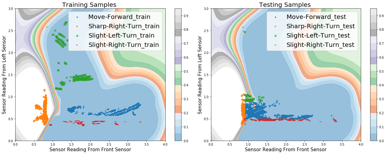
Figure 1. Wall-following navigation task with mobile robot SCITOS-G5 based on sensor readings from the front and left sensor (Dheeru and Karra Taniskidou, 2017).

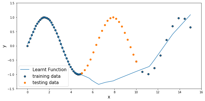
Figure 2. A toy regression example

1.2. Contribution

From the above examples we can observe that ML models work well only in the “training space” (i.e., feature space with sufficient training samples.) Meanwhile, in general, ML models have greater potential to achieve better performance in feature space with more training samples. Therefore, it is essential for safety-critical ML based systems to ensure that their underlying ML modules only work in the training space. As a result, we aim to design a novel technique to do the following job:

1. split the feature space into multiple partitions,

2. identify those in which training samples are insufficient, and

3. reject input instances from these data-lacking feature space partitions.

We first outline the desired characteristics for such a technique:

1. A score function is required to evaluate the resulting feature space partitions.

2. The boundaries of feature space partitions are preferred to be interpretable and understandable, so that we can know, in which partition, ML models may have poor performance. With such information, we can collect more training samples from these regions (if possible).

3. Since we use this technique as a complement to ML models, the output must be generated efficiently, and the additional overhead should be as small as possible.

In this paper, we propose a Feature Space Partitioning Tree (FSPT) with the characteristics mentioned above, which comprises

1. a tree-based classifier for splitting feature space (Section 3) with specific stopping and splitting criterion (Section 4.1 to 4.3.1), and

2. a score function $S(\mathcal{R})$ to evaluate the resulting feature space partitions (Section 4.3.2).

As a toy example, Figure 3 shows the resulting feature space partitions for Example 1. The color of each hyper-rectangle represents the scores from FSPT. As we can see, FSPT gives very low score to most partitions of the feature space because the training data only covers a small portion of the feature space.

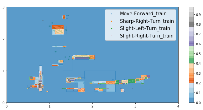
Figure 3. The resulting feature space partitions with scores from FSPT for classification problem in Example 1

Organization: In Section 2 we present related work, and in Section 3, we propose the technique for splitting the feature space into multiple hyper-rectangles based on Classification And Regression Tree (CART) (Breiman et al., 1984). We propose customization techniques (e.g., a new splitting criterion that takes feature importance into consideration and a score function for the resulting feature space partitions) in Section 4. In Section 5, we introduce how to apply FSPT in ML with a reject option. Finally, the experimental results in Section 6 also meet our expectations that, on average, ML models have a higher loss/error rate in feature space partitions with lower FSPT scores. In Table 1, we list notations that will be used in the remainder of this paper.

Table 1. Notations

$\mathbf{Z}=(\mathbf{X},\mathbf{y})$	data set
$\mathbf{X}$	$N\times d$ feature matrix with $N$ samples and $d$ dimensions
$y$	label of an input instance
$\hat{y}$	prediction of an input instance
$\mathbf{y}$	vector of labels
$\mathbf{x}$	feature vector of an input instance
$\mathbf{I}$	a particular feature index
$f_{\mathbf{I}}$	importance of feature $\mathbf{I}$
$\mathbf{x}_{\mathbf{I}}^{k}$	the value of the kth sample in $\mathbf{X}$ on feature $\mathbf{I}$
$\mathcal{R}$	a feature space partition
$\overline{\mathbf{I}}(\mathcal{R})$	upper bound value of feature $\mathbf{I}$ of $\mathcal{R}$
$\underline{\mathbf{I}}(\mathcal{R})$	lower bound value of feature $\mathbf{I}$ of $\mathcal{R}$
$\Delta\mathbf{I}(\mathcal{R})$	$\overline{\mathbf{I}}(\mathcal{R})-\underline{\mathbf{I}}(\mathcal{R})$
$|\mathcal{R}^{+}|$	weighted number of training samples in $\mathcal{R}$
$|\mathcal{R}^{-}|$	weighted number of E-points in $\mathcal{R}$
$G(\mathcal{R})$	Gini index of $\mathcal{R}$
$\hat{G}(\mathcal{R},\mathbf{I},s)$	weighted Gini index with split feature $\mathbf{I}$ and value $s$
$\Delta G(\mathcal{R})$	gain in Gini index
$S(\mathcal{R})$	score of a resulting feature space partition $\mathcal{R}$
$\phi_{F}(\mathbf{x})$	output of FSPT for input instance $\mathbf{x}$
$\phi_{M}(\mathbf{x})$	output of the ML model for input instance $\mathbf{x}$

2. Related Work

In order to determine whether an ML model should select a reject option, we must obtain the “confidence” in its predictive output. For classification problems, the output of an ML model is usually interpreted as its confidence in that prediction. For example, the output obtained at the end of the softmax layers of standard deep learning are often interpreted as the predictive probabilities. For ensemble methods, the weighted votes of the underlying classifiers (Varshney et al., 2013) will be used as the predictive probabilities. As a result, existing works on classification with a reject option (Bartlett and Wegkamp, 2008; Herbei and Wegkamp, 2006) usually determine a reject option based on the predictive output.

An implicit assumption made here is that these classifiers are most uncertain near the decision boundaries of different classes and the distance from the decision boundary is inversely related to the confidence that an input instance belongs to a particular class. This assumption is reasonable in some sense because the decision boundaries learnt by these models are usually located where many training samples with different labels overlap. However, if a feature space $\mathcal{X}$ contains few or no training samples at all, then the decision boundaries of ML models may wholly be based on an inductive bias, thereby having much epistemic uncertainty (Attenberg et al., 2015). In other words, it is possible that an input instance coming from a feature space partition without any training samples would be classified falsely with a very high “predictive probability” by the ML model (Gal and Ghahramani, 2016).

Prediction confidence can also be obtained by Bayesian methods. Unlike classical learning algorithm, Bayesian algorithms do not attempt to identify “best-fit” models of the data. Instead, they compute a posterior distribution over models $P(\theta|\mathbf{X},\mathbf{y})$. For example, Gaussian process (GP) (Seeger, 2004) assumes that $p(f(\mathbf{x}^{1}),\ldots,f(\mathbf{x}^{N}))$ is jointly Gaussian $\mathcal{N}(\mathbf{\mu},\Sigma)$. Given unobserved instance $\mathbf{x}^{*}$, the output $\hat{f}(\mathbf{x}^{*})$ of GP is then also conditional Gaussian $p(\hat{f}(\mathbf{x}^{*})|\mathbf{x}^{*},\mathbf{X},\mathbf{y})=\mathcal{N}(\mu_{*},\sigma_{*})$. The standard deviations $\sigma_{*}$ can then be interpreted as the prediction uncertainty. GP is computationally intensive and has complexity $O(N^{3})$, where N is the number of training samples. Bayesian methods can also be applied to neural networks (NNs). Infinitely wide single hidden layer NNs with distributions placed over their weights converge to Gaussian processes (Neal, 2012). Variational inference (Paisley et al., 2012; Kingma and Welling, 2013) can be used to obtain approximations for finite Bayesian neural networks. The dropout techniques in NNs can also be interpreted as a Bayesian approximation of Gaussian process (Gal and Ghahramani, 2016). Despite the nice properties of Bayesian inference, there are some controversial aspects:

1. The prior plays a key role in computing the marginal likelihood because we are averaging the likelihood over all possible parameter settings $\theta$, as weighted by the prior (Robert, 2014). If the prior is not carefully chosen, we may generate misleading results.

2. It often comes with a high computational cost, especially in models with a large number of parameters.

The conformal prediction framework (Vovk et al., 2005; Vovk et al., 2009) uses past experience to determine precise levels of confidence in new predictions. Given a certain error probability requirement $\epsilon$, it forms a prediction interval $[\overline{f(\mathbf{x})},\underline{{f(\mathbf{x})}}]$ for regression or a prediction label set $\{\mbox{Label 1},\mbox{Label 2},\ldots\}$ for classification so that the interval/set contains the actual prediction with a probability greater than $1-\epsilon$. However, its theoretical correctness depends on the assumption that all the data are independent and identically distributed (later, a weaker assumption of “exchangeability” replaces this assumption). Besides, for regression problems, it tends to produce prediction bands whose width are roughly constant over the whole feature space (Lei et al., 2018).

3. Basic Idea of Partitioning the Feature Space

Our objective is to distinguish the feature space partitions with a high density of training samples from those with a low density of training samples. Let’s assume that there is another category of data points representing the empty feature space (E-points for short) that are uniformly distributed among the entire feature space. As shown in Figure 5, we can use a classifier to distinguish the training data points from E-points. Then, the output of the classifier can be used to indicate whether an input instance is from a feature space partition with sufficient training data.

Figure 4. Decision boundaries of a classifier

Figure 5. Decision boundaries of a tree-based classifier

However, the number of E-points we need to sample will increase exponentially with the number of features. There are two possible solutions to address this issue:

1. apply dimension reduction techniques such as ensembles of low-dimensional sub-models (Nusser et al., 2008) or

2. use tree/rule-based classifiers because their following properties are suitable for our task.

   1. As shown in Figure 5, the feature space partitions constructed by a tree-based classifier are hyper-rectangles. As a result, we can get useful information about each partition, e.g., the side length of each feature, the volume, and the number of training samples within it, very easily.

   2. Suppose the initial feature space $\mathcal{R}$ is split into $\mathcal{R}_{1}$ and $\mathcal{R}_{2}$ by feature $\mathbf{I}$ and value $s$, such that $\forall\mathbf{x}\in\mathcal{R}_{1}:\mathbf{x}_{\mathbf{I}}\leq s$ and $\forall\mathbf{x}\in\mathcal{R}_{2}:\mathbf{x}_{\mathbf{I}}>s$. The number of E-points belonging to $\mathcal{R}_{1}$ and $\mathcal{R}_{2}$ will be in proportion to the side length of feature $\mathbf{I}$, i.e., $\Delta\mathbf{I}(\mathcal{R}_{1})=s-\underline{\mathbf{I}}(\mathcal{R})$ and $\Delta\mathbf{I}(\mathcal{R}_{2})=\overline{\mathbf{I}}(\mathcal{R})-s$ because the E-points are assumed to be uniformly distributed.

Here $\underline{\mathbf{I}}(\mathcal{R})$ and $\overline{\mathbf{I}}(\mathcal{R})$ denote the lower and upper bound values of feature $\mathbf{I}$, respectively. Let $\mathbf{Z}=\left(\mathbf{X},\mathbf{y}\right)$ denote the data set, where $\mathbf{X}$ and $\mathbf{y}$ denote the feature matrix and the vector of labels, respectively, then the lower and upper bound values of feature $\mathbf{I}$ of the entire feature space are as follows.

 Upper Bound  : $$\overline{\mathbf{I}}=\max_{\mathbf{x}\in\mathbf{X}}\mathbf{x}_{\mathbf{I}}$$

 Lower Bound  : $$\underline{\mathbf{I}}=\min_{\mathbf{x}\in\mathbf{X}}\mathbf{x}_{\mathbf{I}}$$

3.1. Tree Construction

In this paper, we consider the classification and regression tree (CART) (Breiman et al., 1984) for feature space partitioning. CART uses Gini index to measure the purity of a feature space partition. Gini index is a measure of how often a randomly chosen element from the set would be incorrectly labeled if it was randomly labeled according to the distribution of labels in the subset. Suppose $|\mathcal{R}^{k}|$ and $|\mathcal{R}|$ denote the weighted number of data points labeled $k$ and the weighted number of all the data points in $\mathcal{R}$, respectively. Then the Gini index of $\mathcal{R}$ can be computed as follows.

(2) $$G(\mathcal{R})=\sum_{k=1}^{K}\frac{|\mathcal{R}^{k}|}{|\mathcal{R}|}\left(1-\frac{|\mathcal{R}^{k}|}{|\mathcal{R}|}\right)$$

Suppose feature space $\mathcal{R}$ is split into $\mathcal{R}_{1}$ and $\mathcal{R}_{2}$ by feature $\mathbf{I}$ and value $s$. CART will always select the split point to minimize the weighted Gini index of $\mathcal{R}_{1}$ and $\mathcal{R}_{2}$.

(3) $$\langle\mathbf{I},~{}s\rangle=\arg\min_{\langle\mathbf{I},~{}s\rangle}\hat{G}(\mathcal{R},\mathbf{I},s),\mbox{ where}$$

$$\hat{G}(\mathcal{R},\mathbf{I},s)=\frac{|\mathcal{R}_{1}|}{|\mathcal{R}|}G(\mathcal{R}_{1})+\frac{|\mathcal{R}_{2}|}{|\mathcal{R}|}G(\mathcal{R}_{2})\\$$

The gain in the Gini index from the split is then

(4) $$\Delta G(\mathcal{R})=G(\mathcal{R})-\min_{\mathbf{I},~{}s}\hat{G}(\mathcal{R},\mathbf{I},s)$$

Let $+$ and $-$ denote the label of training data points and E-points, respectively. Suppose there are infinite E-points uniformly distributed in the hyper-rectangle $\mathcal{R}$. If we set the weight of each E-point to $\frac{|\mathcal{R}^{-}|}{\infty}$, the weighted number of E-points in $\mathcal{R}$ is equal to $\frac{|\mathcal{R}^{-}|}{\infty}\times\infty=|\mathcal{R}^{-}|$. Let $|\mathcal{R}^{+}|$ denote the weighted number of training points in the hyper-rectangle $\mathcal{R}$. The weighted Gini index after $\mathcal{R}$ is split into $\mathcal{R}_{1}$ and $\mathcal{R}_{2}$ is equal to

(5) $$\frac{|\mathcal{R}_{1}^{+}|+|\mathcal{R}_{1}^{-}|}{|\mathcal{R}^{+}|+|\mathcal{R}^{-}|} \times G(\mathcal{R}_{1})+\frac{|\mathcal{R}_{2}^{+}|+|\mathcal{R}_{2}^{-}|}{|\mathcal{R}^{+}|+|\mathcal{R}^{-}|}\times G(\mathcal{R}_{2})~{}\mbox{, where}$$

(6) $$|\mathcal{R}_{1}^{-}| =\frac{s-\underline{\mathbf{I}}(\mathcal{R})}{\overline{\mathbf{I}}(\mathcal{R})-\underline{\mathbf{I}}(\mathcal{R})}\times|\mathcal{R}^{-}|=\frac{s-\underline{\mathbf{I}}(\mathcal{R})}{\Delta{\mathbf{I}}(\mathcal{R})}\times|\mathcal{R}^{-}|$$

(7) $$|\mathcal{R}_{2}^{-}| =\frac{\overline{\mathbf{I}}(\mathcal{R})-s}{\overline{\mathbf{I}}(\mathcal{R})-\underline{\mathbf{I}}(\mathcal{R})}\times|\mathcal{R}^{-}|=\frac{\overline{\mathbf{I}}(\mathcal{R})-s}{\Delta{\mathbf{I}}(\mathcal{R})}\times|\mathcal{R}^{-}|$$

4. CART Customizations for FSPT Feasibility

In this section, we propose several customization techniques for CART to realize FSPT so that it is suitable for identifying feature space partitions without sufficient training samples.

4.1. Stopping Criterion and the Number of E-points

The first question we must answer is when can we stop constructing the tree because otherwise, the tree can grow infinitely. In our case, we can stop further splitting feature space partition $\mathcal{R}$ if all training samples are uniformly distributed in $\mathcal{R}$ approximately. As shown in Figure 6, we can stop splitting $\mathcal{R}_{1}$ and $\mathcal{R}_{2}$ because data points are evenly distributed in them, even though the densities of training samples are different. The intuition for the stopping criterion is that, when the stopping condition is satisfied, any further split can only generate two hyper-rectangles with similar data distributions.

Figure 6. Stop Construction

Another parameter we need to determine is the number of E-points $|\mathcal{R}^{-}|$. According to Equations 6 and 7, the number of E-points $|\mathcal{R}^{-}|$for hyper-rectangle $\mathcal{R}$ could decrease drastically if the split value $s$ is close to the bound of feature $\mathbf{I}$, i.e., $\overline{\mathbf{I}}(\mathcal{R})-s\rightarrow 0$ or $s-\underline{\mathbf{I}}(\mathcal{R})\rightarrow 0$. For a high dimension space, $|\mathcal{R}^{-}|$ will become close to 0 after several splits. As a result, any further division can only result in a negligible decrease in the Gini Index and hence a negligible increase in the gain of Gini Index, which makes it more difficult to find the optimal split point.

To address the above two issues, we fix $|\mathcal{R}^{-}|=|\mathcal{R}^{+}|$ at each split. In this case ($|\mathcal{R}^{+}|=|\mathcal{R}^{-}|$), when the condition, i.e., all training samples are uniformly distributed in $\mathcal{R}$ approximately, is satisfied, the gain in Gini index $\Delta G(\mathcal{R})$ will be close to $0$.

$$\overbrace{G(\mathcal{R})}^{=0.5}-\frac{|\mathcal{R}_{1}|}{|\mathcal{R}|}\times\overbrace{G(\mathcal{R}_{1})}^{\rightarrow 0.5}-\frac{|\mathcal{R}_{2}|}{|\mathcal{R}|}\overbrace{G(\mathcal{R}_{2})}^{\rightarrow 0.5}\rightarrow 0$$

Thus, the gain in Gini index $\Delta G(\mathcal{R})\rightarrow 0$ is a necessary condition to indicate whether the stopping criterion (training samples are evenly distributed in $\mathcal{R}$ approximately) is satisfied. However, it is not a sufficient condition. Figure 7 shows an exceptional scenario where $\Delta G(\mathcal{R})$ is close to $0$, but training samples are not distributed uniformly in $\mathcal{R}$.

To address this issue, we use a counter $c$ to record the number of successive times that $\Delta G(\mathcal{R})\leq\epsilon$ where $\epsilon\rightarrow 0$. The construction process terminates when $c$ is greater than some threshold $\lambda$. For example, in Figure 7, $\Delta G(\mathcal{R})\leq\epsilon$ and hence $c\leftarrow c+1$. After we split $\mathcal{R}$ into $\mathcal{R}_{1}$ and $\mathcal{R}_{2}$,

$$\Delta G(\mathcal{R}_{1})=G(\mathcal{R}_{1})-\frac{|\mathcal{R}_{11}|}{|\mathcal{R}_{1}|}G(\mathcal{R}_{11})-\frac{|\mathcal{R}_{12}|}{|\mathcal{R}_{1}|}G(\mathcal{R}_{12})>\epsilon$$

$$\Delta G(\mathcal{R}_{2})=G(\mathcal{R}_{2})-\frac{|\mathcal{R}_{21}|}{|\mathcal{R}_{2}|}G(\mathcal{R}_{21})-\frac{|\mathcal{R}_{22}|}{|\mathcal{R}_{2}|}G(\mathcal{R}_{22})>\epsilon$$

and hence the counter c is reset to $0$. As a result, the tree construction algorithm will continue to split $\mathcal{R}_{1}\rightarrow\{\mathcal{R}_{11},\mathcal{R}_{12}\}$ and $\mathcal{R}_{2}\rightarrow\{\mathcal{R}_{21},\mathcal{R}_{22}\}$.

Meanwhile, $\lambda$ need not necessarily be a fixed value. When there are lots of training samples in $\mathcal{R}$, then we can assign a larger value to $\lambda$. Otherwise, if $|\mathcal{R}^{+}|$ is very small, the construction process can terminate immediately.

Figure 7. Exceptional Scenario

4.2. Split Points

One of the critical problems in tree learning is to find the best split as represented by Equation 3. A simple greedy solution is to enumerate over all possible split values on all the features. In our case, however, there are infinite possible split values, because we assume there are infinite E-points uniformly distributed in the feature space.

Suppose we want to find the best split for the hyper-rectangle $\mathcal{R}$ on feature $\mathbf{I}$. Let $\mathcal{S}_{\mathbf{I}}=\{s_{1},s_{2},\ldots,s_{N}\}$ denote the set of unique values of feature $\mathbf{I}$ of training samples in $\mathcal{R}$, where items in $\mathcal{S}_{\mathbf{I}}$ are sorted in ascending order, i.e., $\underline{\mathbf{I}}(\mathcal{R})\leq s_{1}<\ldots<s_{N}\leq\overline{\mathbf{I}}(\mathcal{R})$. Let $\mbox{cdf}(s)$ denote the cumulative distribution function of training samples in $\mathcal{R}$ on feature $\mathbf{I}$. Then $\forall s\in[s_{k},s_{k+1})$, we have $\mbox{cdf}(s)=\mbox{cdf}(s_{k})$ because there exists no training sample with feature $\mathbf{I}$ within $(s_{k},s_{k+1})$. For simplicity, we assume feature $\mathbf{I}$ is normalized to 1, i.e., $\Delta\mathbf{I}(\mathcal{R})=\overline{\mathbf{I}}(\mathcal{R})-\underline{\mathbf{I}}(\mathcal{R})=1$, and hence the split value $s\in[0,1]$. If we split $\mathcal{R}$ into $\mathcal{R}_{1}$ and $\mathcal{R}_{2}$ by value $s$ and feature $\mathbf{I}$, then

$$G(\mathcal{R}_{1})=2\times\left(\frac{|\mathcal{R}_{1}^{+}|}{|\mathcal{R}_{1}^{+}|+|\mathcal{R}_{1}^{-}|}\right)\left(\frac{|\mathcal{R}_{1}^{-}|}{|\mathcal{R}_{1}^{+}|+|\mathcal{R}_{1}^{-}|}\right)$$

$$=2\left(\frac{\mbox{cdf}(s)}{\mbox{cdf}(s)+s}\right)\left(\frac{s}{\mbox{cdf}(s)+s}\right)$$

$$G(\mathcal{R}_{2})=2\times\left(\frac{|\mathcal{R}_{2}^{+}|}{|\mathcal{R}_{2}^{+}|+|\mathcal{R}_{2}^{-}|}\right)\left(\frac{|\mathcal{R}_{2}^{-}|}{|\mathcal{R}_{2}^{+}|+|\mathcal{R}_{2}^{-}|}\right)$$

$$=2\left(\frac{1-\mbox{cdf}(s)}{2-\mbox{cdf}(s)-s}\right)\left(\frac{1-s}{2-\mbox{cdf}(s)-s}\right)$$

$$\Rightarrow\hat{G}(\mathcal{R},\mathbf{I},s)=\frac{\mbox{cdf}(s)+s}{2}\times G(\mathcal{R}_{1})+\frac{2-s-\mbox{cdf}(s)}{2}\times G(\mathcal{R}_{2})$$

$$=\left(\frac{\mbox{cdf}(s)s}{\mbox{cdf}(s)+s}\right)+\left(\frac{(1-\mbox{cdf}(s))(1-s)}{2-\mbox{cdf}(s)-s}\right)$$

Let’s compute the partial derivative of weighted Gini index on $s$.

$$\frac{\partial\hat{G}(\mathcal{R},\mathbf{I},s)}{\partial s}=\left(\frac{\mbox{cdf}(s)}{\mbox{cdf}(s)+s}\right)^{2}-\left(\frac{1-\mbox{cdf}(s)}{2-\mbox{cdf}(s)-s}\right)^{2}=$$

$$\overbrace{\left(\!\!\frac{\mbox{cdf}(s)}{\mbox{cdf}(s)+s}\!+\!\frac{1-\mbox{cdf}(s)}{2-\mbox{cdf}(s)-s}\!\!\right)}^{>0}\!\!\left(\!\!\frac{\mbox{cdf}(s)-s}{(\mbox{cdf}(s)+s)(2-\mbox{cdf}(s)-s)}\!\!\right)$$

When $s\in[s_{k},s_{k+1})$, $\mbox{cdf}(s)=\mbox{cdf}(s_{k})$ is a constant value. If $s_{k}\geq\mbox{cdf}(s_{k})\Rightarrow\frac{\partial\hat{G}(\mathcal{R},\mathbf{I},s)}{\partial s}\leq 0$, then $\hat{G}(\mathcal{R},\mathbf{I},s)$ is minimized when $s=s_{k+1}-\epsilon$, where $\epsilon\rightarrow+0$. If $s_{k+1}\leq\mbox{cdf}(s_{k})\Rightarrow\frac{\partial\hat{G}(\mathcal{R},\mathbf{I},s)}{\partial s}\geq 0$, then $\hat{G}(\mathcal{R},\mathbf{I},s)$ is minimized when $s=s_{k}$. Finally if $s_{k}<\mbox{cdf}(s_{k})<s_{k+1}$, then $\hat{G}(\mathcal{R},\mathbf{I},s)$ is minimized when $s=s_{k}$ or $s=s_{k+1}-\epsilon$.

Therefore, there is no need to try all infinite split values, and the potential split value set is reduced to

$$\left\{\max\left(\underline{\mathbf{I}}(\mathcal{R}),s_{1}-\epsilon\right),s_{1},s_{2}-\epsilon,s_{2},s_{3}-\epsilon,\ldots,s_{N}\right\}$$

It can still be computationally demanding to enumerate all the split points in the candidate set, especially when the data cannot fit entirely into memory. To address this issue, we can also use approximate split finding algorithms (e.g., use candidate splitting points according to percentiles of feature distribution), which is quite common in tree learning algorithms.

4.3. New Splitting Criterion and Score Function

In general, more training samples are required for an ML model to achieve good performance within a feature space partition $\mathcal{R}$ with a larger volume $V(\mathcal{R})$, where

$$V(\mathcal{R})=\prod_{\mathbf{I}}\left(\overline{\mathbf{I}}(\mathcal{R})-\underline{\mathbf{I}}(\mathcal{R})\right)=\prod_{\mathbf{I}}\Delta\mathbf{I}(\mathcal{R})$$

This scenario is clearly shown in Example 2 in Section 1.1. While two feature space partitions $x\in[0,5]$ and $x\in(10,15]$ have the same volume, the ML model fits the sine function much better in the former with 40 training samples than in the latter with 10 training samples. Of course, this is not always the case, especially when the model is poorly trained. For example, imagine we have a model whose output is always zero. Then it is evident that its performance has a very weak dependence on the training samples. Thus, the premise to infer ML models’ performance in different feature space partitions from training samples and volume $V(\mathcal{R})$ is that it does not over-fit or under-fit.

Another challenge in inferring ML models’ performance in $\mathcal{R}$ from its volume and training samples is that all features are equally important in the computation of volume. Besides, as long as there exists any feature $\mathbf{I}$ with $\Delta\mathbf{I}(\mathcal{R})$ close to 0, the volume of $\mathcal{R}$ will also be close to 0 irrespective of the feature importance of $\mathbf{I}$ and the side length of other features.

As shown in Figure 9, $\mathcal{R}_{1}$ and $\mathcal{R}_{2}$ have the same number of training samples, but $\mathcal{R}_{1}$ covers a larger feature space. If feature $x$ and feature $y$ are equally important, then we can expect that an ML model will have a higher fitting degree of the objective function in $\mathcal{R}_{2}$ than in $\mathcal{R}_{1}$, if it does not over-fit or under-fit. However, if feature $y$ is of very low importance or irrelevant to the objective function, then the previous inference can be misleading.

To address this problem, we can exclude all the irrelevant features, and meanwhile, incorporate feature importance into the splitting criterion as well as the score function for the resulting feature space partitions. There are lots of techniques that can be used to assess feature importance (Gevrey et al., 2003; Williamson et al., 2017; Breiman, 2001). Of course, it is not trivial to obtain precise feature importance values. Meanwhile, features that are globally important may not be important in the local context, and vice versa. In this paper, we only consider global feature importance with constant values.

Figure 8. Problem of Irrelevant Features

Figure 9. Resulting hyper-rectangles have too small rectangles

Another issue is that we also do not want to split the feature space into too many hyper-rectangles with an extremely small side length on a particular feature $\mathbf{I}$, i.e., $\frac{\Delta\mathbf{I}(\mathcal{R})}{\Delta\mathbf{I}}\rightarrow 0$, where $\Delta\mathbf{I}$ is the side length of the entire feature space. For example, in Figure 9, since $\frac{\Delta\mathbf{I}(\mathcal{R})}{\Delta\mathbf{I}}=0.3\%\rightarrow 0$, we will not further split on this feature unless it can bring significant gain in the splitting criterion.

To meet the requirements mentioned above, we propose:

1. A more reasonable splitting criterion named weighed gain in Gini index, which considers 1) $\hat{G}(\mathcal{R},\mathbf{I},s)$, 2) the feature importance values $\{f_{1},f_{2},\ldots,f_{d}\}$ and 3) the side length of each feature $\Delta\mathbf{I}(\mathcal{R})$.

2. A heuristic score function to assess the resulting feature space partitions.

4.3.1. Splitting Criterion

Equation 8 shows the new criterion for selecting splitting points.

(8) $$\langle\mathbf{I},~{}s\rangle=\arg\max_{\langle\mathbf{I},~{}s\rangle}\frac{f_{\mathbf{I}}\times\Delta\mathbf{I}(\mathcal{R})}{\Delta\mathbf{I}}\Delta G(\mathcal{R})\\$$

$$\mbox{where }\Delta G(\mathcal{R})=\left(G(\mathcal{R})-\hat{G}(\mathcal{R},\mathbf{I},s)\right)$$

The intuition of this criterion is simple. We prefer to split on features that are important and have a larger side length, unless there is a significant increase in $\Delta G(\mathcal{R})$.

4.3.2. Score Function

We propose a heuristic score function in Equation 9 to evaluate the resulting hyper-rectangle $\mathcal{R}$, and it takes both the feature importance and the side length of each feature into consideration.

(9) $$S(\mathcal{R})=\sum_{\mathbf{I}}f_{\mathbf{I}}\times\frac{|\mathcal{R}^{+}|}{|\mathcal{R}^{+}|+\frac{\Delta\mathbf{I}(\mathcal{R})}{\Delta\mathbf{I}}\times E}$$

In Equation 9, $E$ is a hyperparameter. We set $E=\frac{N}{d}$ in our experiments in Section 6, where $N$ is the number of training samples and $d$ is the number of features. The intuition for Equation 9 is that we evaluate $\mathcal{R}$ on each feature separately based the training samples and side length $\Delta\mathbf{I}(\mathcal{R})$. For example, if $\Delta\mathbf{I}(\mathcal{R})\rightarrow 0$, i.e., training samples in $\mathcal{R}$ have the same value on feature $\mathbf{I}$, then $\mathcal{R}$ is supposed to get the full score of feature $\mathbf{I}$ (i.e., $f_{\mathbf{I}}$). After FSPT completes the tree construction, the final scores for each partition can be normalized into the range $[0,1]$.

Complexity: Suppose FSPT has depth $T$, then the score of an input instance can be calculated efficiently with complexity $O(T)$. Since each feature space partition contains at least one training sample, the run-time complexity is $O(\log N)$

5. Reject Model

Suppose input instance $x$ is in feature space partition $\mathcal{R}$, the output of FSPT for $x$ is

$$\phi_{F}(x)=S(\mathcal{R})$$

Regression Problems: We can use $\phi_{F}(x)$ to determine whether the prediction for input instance $x$ should be rejected in regression problems directly. Let $\phi_{M}(x)$ denote the predictive output of ML models for input instance $x$, then a reject option can be selected when $\phi_{F}(x)$ is smaller than a particular threshold $t$.

(10) $$\hat{y}(x)=\begin{cases}\phi_{M}(x)~{}\mbox{ if }\phi_{F}(x)\geq t\\ \mbox{reject option, otherwise }\end{cases}$$

Classification Problems: Suppose $\phi_{M}^{c}(x)$ denotes ML models’ predictive probability that $x$ belongs to class “c”, then the final predictive class for $x$ is

$$c=\arg\max_{c}\{\phi_{M}^{c}(x)\}$$

Let $\phi_{M}(x)=\max_{c}\{\phi_{M}^{c}(x)\}$, we use both $\phi_{M}(x)$ and $\phi_{F}(x)$ to determine whether a reject option should be selected. The reason to adopt such a reject strategy is that an ML model’s accuracy for an input instance depends on its distance to the decision boundaries significantly.

Figure 10 shows a toy example of a binary classification problem. As we can see, few training samples exist in feature space partition $\mathcal{R}_{1}$ and $\mathcal{R}_{2}$ perhaps due to small probability density there. Thus, FSPT gives relatively low scores to $\mathcal{R}_{1}$ and $\mathcal{R}_{2}$ because there is not sufficient evidence to draw a confident conclusion.

Figure 10. Training samples for a binary classification problem

However, the model may have $100\%$ accuracy in $\mathcal{R}_{1}$ and $\mathcal{R}_{2}$ just because its guess is “lucky” enough to be correct.

Thus, for classification problems, the output of FSPT will be used as a complement to the ML model, and the prediction of ML models will be adopted only when both $\phi_{F}(x)$ and $\phi_{M}^{c}(x)$ exceed the corresponding thresholds.

(11) $$\hat{y}(x)=\begin{cases}c~{}\mbox{ if }\phi_{M}^{c}(x)\geq t_{1}\wedge\phi_{F}(x)\geq t_{2}\\ \mbox{reject option, otherwise }\end{cases}$$

6. Evaluation

In this section, we evaluate the effectiveness of our proposed technique for both regression and classification problems. The feature importance values used in the experiments are obtained from Random Forest (Breiman, 2001). We investigate the performance of three popular ML models, i.e.,

1. Neural Networks (NN)

2. Support Vector Machine (SVM)

3. Gaussian Process (GP)

when we set different rejection thresholds for them. Since GP can offer standard deviations for testing samples in regression problems, we also investigate the relationship between the standard deviations and $\phi_{F}(x)$. For a given data set $\mathbf{Z}$, testing samples are randomly sampled from $\mathbf{Z}$. In Figure 11, 16, 21 and 22, we show the distributions of testing samples with respect to the scores.

6.1. Regression Problems

For regression problems, we evaluate the reject model in Equation 10. We use box-plot (Figure 12 to 20) to show absolute loss $|y-\hat{y}|$/standard deviation of testing samples with different rejection thresholds $t\in\{0,0.1,0.2,0.3,\ldots,1\}$. We consider the following two applications in the experiments.

Quality Prediction in a Mining Process: This dataset is about a flotation plant which is a process used to concentrate the iron ore (min, [n.d.]). The goal of this task is to predict the percentage of Silica at the end of the process from 22 features. As this value is measured every hour, if we can predict how much silica is in the ore concentrate, we can help the engineers, giving them early information to take actions. Hence, they will be able to take corrective actions in advance and also help the environment by reducing the amount of ore that goes to tailings.

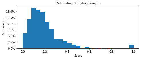
Figure 11. Mining Process: sample distribution

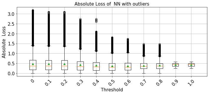
Figure 12. Mining Process: absolute loss for NNs

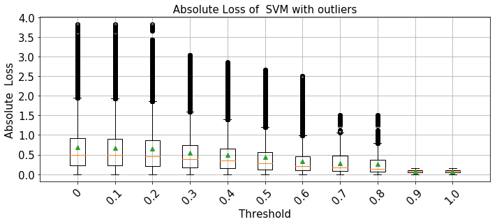
Figure 13. Mining Process: absolute loss for SVM

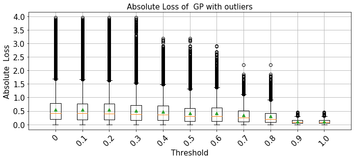
Figure 14. Mining Process: absolute loss for GP

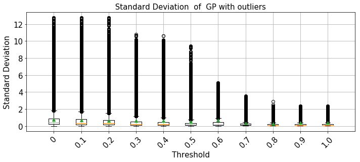
Figure 15. Mining Process: standard deviation for GP

The Inverse Dynamics of a SARCOS Robot Arm: This task is to map from a 21-dimensional input space (7 joint positions, 7 joint velocities, 7 joint accelerations) from a seven degrees-of-freedom SARCOS robot arm (SAR, [n.d.]) to the inverse dynamics of a corresponding torque. An inverse dynamics model can be used in the following manner: a planning module decides on a trajectory that takes the robot from its start to goal states, and this specifies the desired positions, velocities and accelerations at each time. The inverse dynamics model is used to compute the torques needed to achieve this trajectory and errors are corrected using a feedback controller (Seeger, 2004).

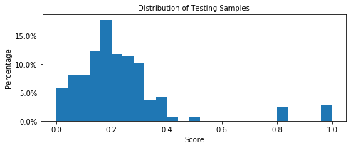
Figure 16. SARCO: sample distribution

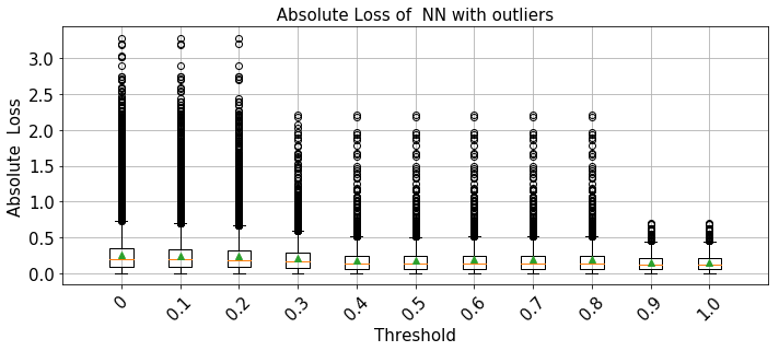
Figure 17. SARCO: absolute loss for NNs

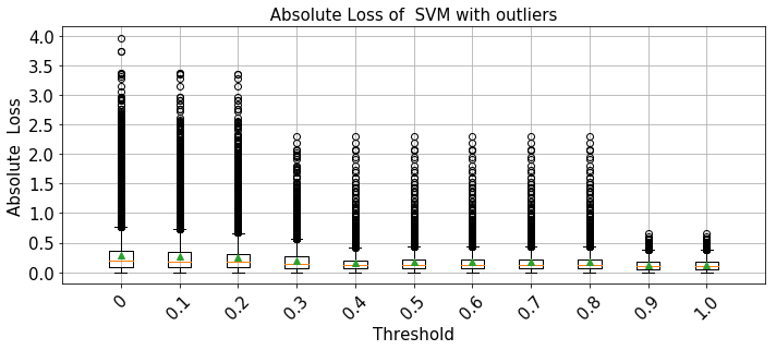
Figure 18. SARCO: absolute loss for SVM

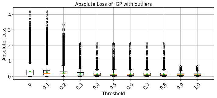
Figure 19. SARCO: absolute loss for GP

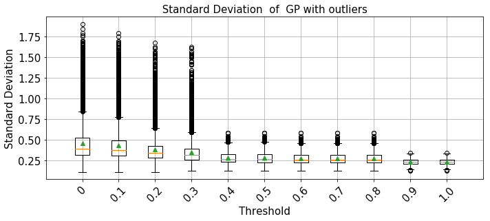
Figure 20. SARCO: standard deviation for GP

6.2. Classification Problems

For classification problems, we evaluate the reject model in Equation 11. Through the experiment results, we show that input instance with both high scores from FSPT $\phi_{F}(x)$ and high scores (i.e., predictive probability output $\phi_{M}(x)$) from ML models has a lower error rate. Let $t_{1}$ denote the rejection threshold for ML model, and $t_{2}$ denote rejection threshold for FSPT. We partition testing samples into group $G_{1}$ and $G_{2}$.

1. $G_{1}$: $\phi_{M}(x)\geq t_{1}\wedge\phi_{F}(x)\geq t_{2}$

2. $G_{2}$: $\phi_{M}(x)\geq t_{1}\wedge\phi_{F}(x)<t_{2}$

From Table 2 to Table 7, we present the accuracy of $G_{1}$ and $G_{2}$ for different combinations of $t_{1}$ and $t_{2}$. Besides, we also show the mean value of $\phi_{M}(x)$ and proportion of $G_{1}$ and $G_{2}$. We show that even when $G_{1}$ and $G_{2}$ have similar mean values of $\phi_{M}(x)$, which indicates that ML models have similar confidence in the predictions of the testing samples in $G_{1}$ and $G_{2}$, their accuracy of $G_{1}$ is higher than $G_{2}$. We consider the following two applications in the experiments.

The Navigation Task for Mobile Robot SCITOS-G5: This task is to map 24-dimension input, i.e., sensor readings from the 24 sensors of the mobile robot SCITOS-G5 (Dheeru and Karra Taniskidou, 2017) to 4 classes of behaviors: 1) “Move-Forward”, 2) “Sharp-Right-Turn”, 3) “Slight-Left-Turn” and 4) “Slight-Right-Turn”. ML models will be trained for the mobile robot to take decisions that determine its correct movement.

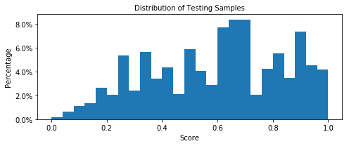
Figure 21. SCITOS: sample distribution

Table 2. SCITOS: NNs

$t_{1}~{}t_{2}$	$G_{1}$			$G_{2}$
	Proportion	Accuracy	$\phi_{M}(x)$	Proportion	Accuracy	$\phi_{M}(x)$
0.90 0.00	1.00	0.925	0.970	0.00	nan	nan
0.90 0.30	0.86	0.925	0.970	0.14	0.921	0.972
0.90 0.60	0.55	0.930	0.970	0.45	0.918	0.970
0.90 0.90	0.14	0.931	0.972	0.86	0.924	0.970
0.95 0.00	1.00	0.947	0.984	0.00	nan	nan
0.95 0.30	0.85	0.948	0.984	0.15	0.944	0.984
0.95 0.60	0.54	0.951	0.984	0.46	0.942	0.984
0.95 0.90	0.15	0.956	0.984	0.85	0.946	0.984

Table 3. SCITOS: SVM

$t_{1}~{}t_{2}$	$G_{1}$			$G_{2}$
	Proportion	Accuracy	$\phi_{M}(x)$	Proportion	Accuracy	$\phi_{M}(x)$
0.90 0.00	1.00	0.960	0.963	0.00	nan	nan
0.90 0.30	0.86	0.961	0.963	0.14	0.954	0.962
0.90 0.60	0.56	0.967	0.962	0.44	0.950	0.963
0.90 0.90	0.15	0.959	0.961	0.85	0.960	0.963
0.95 0.00	1.00	0.968	0.979	0.00	nan	nan
0.95 0.30	0.86	0.970	0.979	0.14	0.958	0.979
0.95 0.60	0.56	0.975	0.978	0.44	0.959	0.980
0.95 0.90	0.14	0.974	0.978	0.86	0.967	0.979

Table 4. SCITOS: GP

$t_{1}~{}t_{2}$	$G_{1}$			$G_{2}$
	Proportion	Accuracy	$\phi_{M}(x)$	Proportion	Accuracy	$\phi_{M}(x)$
0.60 0.00	1.00	0.975	0.703	0.00	nan	nan
0.60 0.30	0.52	0.989	0.712	0.48	0.960	0.694
0.60 0.60	0.12	1.000	0.738	0.88	0.972	0.698
0.60 0.90	0.02	1.000	0.782	0.98	0.975	0.702
0.70 0.00	1.00	0.989	0.761	0.00	nan	nan
0.70 0.30	0.58	0.989	0.762	0.42	0.989	0.761
0.70 0.60	0.18	1.000	0.764	0.82	0.986	0.761
0.70 0.90	0.03	1.000	0.785	0.97	0.989	0.761

Breast Cancer Diagnosis: This task is to map 30 features computed from a digitized image of a fine needle aspirate (FNA) of a breast mass to Class “benign” and Class “malignant” (bre, [n.d.]).

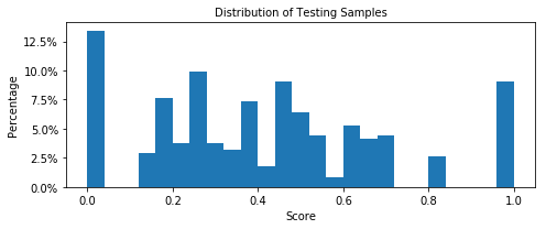
Figure 22. Breast Cancer Diagnosis: sample distribution

Table 5. Breast Cancer Diagnosis: NNs

$t_{1}~{}t_{2}$	$G_{1}$			$G_{2}$
	Proportion	Accuracy	$\phi_{M}(x)$	Proportion	Accuracy	$\phi_{M}(x)$
0.80 0.00	1.00	0.892	0.990	0.00	nan	nan
0.80 0.20	0.75	0.916	0.992	0.25	0.821	0.981
0.80 0.40	0.48	0.907	0.994	0.52	0.879	0.986
0.80 0.60	0.26	0.926	0.993	0.74	0.881	0.988
0.90 0.00	1.00	0.899	0.994	0.00	nan	nan
0.90 0.20	0.76	0.914	0.996	0.24	0.849	0.990
0.90 0.40	0.48	0.905	0.997	0.52	0.892	0.992
0.90 0.60	0.26	0.924	0.997	0.74	0.890	0.993

Table 6. Breast Cancer Diagnosis: SVM

$t_{1}~{}t_{2}$	$G_{1}$			$G_{2}$
	Proportion	Accuracy	$\phi_{M}(x)$	Proportion	Accuracy	$\phi_{M}(x)$
0.80 0.00	1.00	0.988	0.936	0.00	nan	nan
0.80 0.20	0.77	0.995	0.938	0.23	0.966	0.928
0.80 0.40	0.47	0.992	0.942	0.53	0.985	0.930
0.80 0.60	0.27	0.985	0.944	0.73	0.989	0.933
0.90 0.00	1.00	0.995	0.964	0.00	nan	nan
0.90 0.20	0.78	1.000	0.966	0.22	0.976	0.959
0.90 0.40	0.48	1.000	0.971	0.52	0.990	0.958
0.90 0.60	0.28	1.000	0.969	0.72	0.993	0.962

Table 7. Breast Cancer Diagnosis: GP

$t_{1}~{}t_{2}$	$G_{1}$			$G_{2}$
	Proportion	Accuracy	$\phi_{M}(x)$	Proportion	Accuracy	$\phi_{M}(x)$
0.55 0.00	1.00	0.940	0.914	0.00	nan	nan
0.55 0.20	0.76	0.944	0.913	0.24	0.925	0.920
0.55 0.40	0.48	0.943	0.899	0.52	0.937	0.928
0.55 0.60	0.25	0.964	0.912	0.75	0.932	0.915
0.60 0.00	1.00	0.948	0.923	0.00	nan	nan
0.60 0.20	0.76	0.955	0.922	0.24	0.924	0.924
0.60 0.40	0.47	0.954	0.910	0.53	0.942	0.934
0.60 0.60	0.25	0.975	0.925	0.75	0.939	0.922

6.3. Short Summary:

As we can observe from the experimental results in this section, a strong relationship exists between the ML model’s performance and the scores $\phi_{F}(x)$ from FSPT. In regression problems, we can reduce both mean error and maximum error, and thereby improve the reliability of ML models, by rejecting predictions with very small $\phi_{F}(x)$. In classification problems, by rejecting input instances with either low FSPT score or ML model score, the prediction accuracy can also be improved. Even among the predictions in which ML models have similar confidence (i.e., predictions with similar predictive probability $\phi_{M}(x)$), the error rate of those with higher $\phi_{F}(x)$ is lower than the rest.

7. Conclusion

In this paper, we propose a feature space partition tree (FSPT) to split the feature space into multiple partitions with different training data densities. The resulting feature space partitions are scored using a heuristic metric based on the principle that an ML model’s performance in a particular feature space partition $\mathcal{R}$ is upper bounded by the training samples within $\mathcal{R}$. Based on FSPT, we propose two rejection models for regression and classification problems, respective. The preliminary experimental results in Section 6 also meet our expectations. However, the current version of FSPT has many limitations to be addressed:

1. First, the criterion to construct FSPT depends on the feature importance or model’s reliance on different features. However, it is not a trivial task to get accurate feature importance values. Besides, features that are globally important may not be important in the local context, and vice versa. Thus, one possible direction to improve FSPT is to incorporate local feature importance in it.

2. Another major limitation is that FSPT is only suitable for low-dimension tabular data sets. For complex input data such as images, we should apply FSPT to more meaningful features extracted by other techniques rather than pixel values. For example, DNN trained on images can extract eyes, tail etc. as features in their last layers.

3. Besides, since the score function is heuristic, we can only show that a strong relationship exists between model performance and FSPT score. In the future, we also plan to derive a more accurate score function.

4. Finally, we also need to derive a threshold for reject option for a required confidence level. Perhaps, we can apply the conformal prediction framework (Vovk et al., 2005; Vovk et al., 2009) in the different feature space partitions locally, and derive a threshold for a certain error probability requirement.

- (1)
- bre ([n.d.]) [n.d.]. Breast Cancer Wisconsin (Diagnostic) Data Set. https://www.kaggle.com/uciml/breast-cancer-wisconsin-data/home
- min ([n.d.]) [n.d.]. Quality Prediction in a Mining Process. https://www.kaggle.com/edumagalhaes/quality-prediction-in-a-mining-process
- SAR ([n.d.]) [n.d.]. SARCOS. http://www.gaussianprocess.org/gpml/data/
- Attenberg et al. (2015) Joshua Attenberg, Panos Ipeirotis, and Foster Provost. 2015. Beat the Machine: Challenging Humans to Find a Predictive Model’s &Ldquo;Unknown Unknowns&Rdquo;. J. Data and Information Quality 6, 1 (2015), 1:1–1:17.
- Bartlett and Wegkamp (2008) Peter L Bartlett and Marten H Wegkamp. 2008. Classification with a reject option using a hinge loss. Journal of Machine Learning Research 9, Aug (2008), 1823–1840.
- Bojarski et al. (2016) Mariusz Bojarski, Davide Del Testa, Daniel Dworakowski, Bernhard Firner, Beat Flepp, Prasoon Goyal, Lawrence D Jackel, Mathew Monfort, Urs Muller, Jiakai Zhang, et al. 2016. End to end learning for self-driving cars. arXiv preprint arXiv:1604.07316 (2016).
- Breiman (2001) Leo Breiman. 2001. Random forests. Machine learning 45, 1 (2001), 5–32.
- Breiman et al. (1984) Leo Breiman, Jerome H Friedman, Richard A Olshen, and Charles J Stone. 1984. Classification and regression trees. Wadsworth & Brooks/Cole Advanced Books & Software.
- Dheeru and Karra Taniskidou (2017) Dua Dheeru and Efi Karra Taniskidou. 2017. UCI Machine Learning Repository. http://archive.ics.uci.edu/ml
- Gal and Ghahramani (2016) Yarin Gal and Zoubin Ghahramani. 2016. Dropout as a Bayesian approximation: Representing model uncertainty in deep learning. In international conference on machine learning. 1050–1059.
- Gevrey et al. (2003) Muriel Gevrey, Ioannis Dimopoulos, and Sovan Lek. 2003. Review and comparison of methods to study the contribution of variables in artificial neural network models. Ecological modelling 160, 3 (2003), 249–264.
- Herbei and Wegkamp (2006) Radu Herbei and Marten H Wegkamp. 2006. Classification with reject option. Canadian Journal of Statistics 34, 4 (2006), 709–721.
- Jain et al. (2018) Achin Jain, Truong X Nghiem, Manfred Morari, and Rahul Mangharam. 2018. Learning and control using gaussian processes: towards bridging machine learning and controls for physical systems. In Proceedings of the 9th ACM/IEEE International Conference on Cyber-Physical Systems. IEEE Press, 140–149.
- Kingma and Welling (2013) Diederik P Kingma and Max Welling. 2013. Auto-encoding variational bayes. arXiv preprint arXiv:1312.6114 (2013).
- Lei et al. (2018) Jing Lei, Max G’Sell, Alessandro Rinaldo, Ryan J Tibshirani, and Larry Wasserman. 2018. Distribution-free predictive inference for regression. J. Amer. Statist. Assoc. (2018), 1–18.
- Lin et al. (2005) Henry C Lin, Izhak Shafran, Todd E Murphy, Allison M Okamura, David D Yuh, and Gregory D Hager. 2005. Automatic detection and segmentation of robot-assisted surgical motions. In International Conference on Medical Image Computing and Computer-Assisted Intervention. Springer, 802–810.
- Marcus (2018) Gary Marcus. 2018. Deep learning: A critical appraisal. arXiv preprint arXiv:1801.00631 (2018).
- Neal (2012) Radford M Neal. 2012. Bayesian learning for neural networks. Vol. 118. Springer Science & Business Media.
- Nusser et al. (2008) Sebastian Nusser, Clemens Otte, and Werner Hauptmann. 2008. Interpretable ensembles of local models for safety-related applications.. In ESANN. 301–306.
- Paisley et al. (2012) John Paisley, David Blei, and Michael Jordan. 2012. Variational Bayesian inference with stochastic search. arXiv preprint arXiv:1206.6430 (2012).
- R. Varshney and Alemzadeh (2016) Kush R. Varshney and Homa Alemzadeh. 2016. On the Safety of Machine Learning: Cyber-Physical Systems, Decision Sciences, and Data Products. 5 (10 2016).
- Ribeiro and Guestrin (2016) Sameer Singh Ribeiro, Marco Tulio and Carlos Guestrin. 2016. Why should i trust you?: Explaining the predictions of any classifier. (2016).
- Robert (2014) Christian Robert. 2014. Machine learning, a probabilistic perspective.
- Salay et al. (2017) Rick Salay, Rodrigo Queiroz, and Krzysztof Czarnecki. 2017. An Analysis of ISO 26262: Using Machine Learning Safely in Automotive Software. CoRR abs/1709.02435 (2017). arXiv:1709.02435 http://arxiv.org/abs/1709.02435
- Seeger (2004) Matthias Seeger. 2004. Gaussian processes for machine learning. International journal of neural systems 14, 02 (2004), 69–106.
- Udeshi et al. (2018) Sakshi Udeshi, Pryanshu Arora, and Sudipta Chattopadhyay. 2018. Automated directed fairness testing. Proceedings of the 33rd ACM/IEEE International Conference on Automated Software Engineering - ASE 2018 (2018). https://doi.org/10.1145/3238147.3238165
- Varshney et al. (2013) Kush R Varshney, Ryan J Prenger, Tracy L Marlatt, Barry Y Chen, and William G Hanley. 2013. Practical ensemble classification error bounds for different operating points. IEEE Transactions on Knowledge and Data Engineering 25, 11 (2013), 2590–2601.
- Vovk et al. (2005) Vladimir Vovk, Alex Gammerman, and Glenn Shafer. 2005. Algorithmic Learning in a Random World. Springer-Verlag, Berlin, Heidelberg.
- Vovk et al. (2009) Vladimir Vovk, Ilia Nouretdinov, Alex Gammerman, et al. 2009. On-line predictive linear regression. The Annals of Statistics 37, 3 (2009), 1566–1590.
- Weiss (1995) Gary M Weiss. 1995. Learning with rare cases and small disjuncts. (1995), 558–565.
- Weiss (2004) Gary M Weiss. 2004. Mining with rarity: a unifying framework. ACM Sigkdd Explorations Newsletter 6, 1 (2004), 7–19.
- Williamson et al. (2017) Brian D Williamson, Peter B Gilbert, Noah Simon, and Marco Carone. 2017. Nonparametric variable importance assessment using machine learning techniques. (2017).