Fractional hyperviscosity induced growth of bottlenecks in energy spectrum of Burgers equation solutions

Abstract

Energy spectrum of turbulent fluids exhibit a bump at an intermediate wavenumber, between the inertial and the dissipation range. This bump is called bottleneck. Such bottlenecks are also seen in the energy spectrum of the solutions of hyperviscous Burgers equation. Previous work, have shown that this bump corresponds to oscillations in real space velocity field. In this paper we present numerical and analytical results of how the bottleneck and its’ real space signature, the oscillations, grow as we tune the order of hyperviscosity. We look at a parameter regime $\alpha\in[1,2]$ where $\alpha=1$ corresponds to normal viscosity and $\alpha=2$ corresponds to hyperviscosity of order 2. We show that even for the slightest fractional increment in the order of hyperviscosity ($\alpha$) bottlenecks show up in the energy spectrum.

1 Introduction

High resolution direct numerical simulations and experimental data have shown the presence of bottleneck in the kinetic energy spectrum  Kaneda2003 ; Dobler2003 ; Beresnyak2011 ; Donzis2010 . The energy spectrum is defined as $E(k)\equiv 1/\Delta\Sigma_{{\bf k}\in[k,k+\Delta]}{\bf v}({\bf k})^{2}$, where, ${\bf v}$ is the velocity field of the turbulent fluid. Typical fluid turbulence energy spectrum is characterised by two length scales – the large length scale at which energy is injected in the flow, the corresponding wave number being $k_{\rm inj}$, and the small length scale at which the energy dissipation due to viscosity becomes important and corresponds to a wavenumber $k_{\rm diss}$. Now, in between these wavenumbers we have the inertial range and is characterised by a scaling behaviour in the energy spectrum i.e. for $k_{\rm inj}\ll k\ll k_{\rm diss}$ we have $E(k)\sim k^{-5/3}$ where the exponent $5/3$ corresponds to the Kolmogorov exponent Kolmogorov1941 ; Frisch1995 . In the solutions of Burgers equation one can also define an inertial range but with a scaling behaviour given by $E(k)\sim k^{-2}$. Bottleneck is characterised by the presence of a bump at an intermediate wavenumber, between the inertial and the dissipation wavenumbers. The bump in this intermediate wavenumber occurs due to an inefficient transfer of energy across wavenumbers Falkovich1994 and manifests as oscillation in the real space correlation functions Frisch2013 . Another aspect of bottlenecks that has been discussed in literature before is the fact that the effect of bottlenecks gets more pronounced if one uses hyperviscosity instead of viscosity. To get a clearer theoretical understanding of the bottlenecks one needs to consider the one dimensional Burgers equation Burgers1948 ; Bec2007 ; Bec2002 ; Frisch2002 in the presence of hyperviscosity. It has been shown in Ref. Frisch2013 that oscillations emerge in the solutions of Burgers equation in the presence of hyperviscosity which can be causally related to the bottlenecks in the energy spectrum. However, unlike fluid turbulence it can also be shown that these oscillations vanish in the limit of a normal viscous Burgers equation Frisch2013 ; Frisch2008 ; Banerjee2014 .

The use of hyperviscosity, to introduce strong dissipation at large wavenumbers leading to an extended inertial range behaviour, have been a common practice in direct numerical simulations of turbulence. In the usage of hyperviscosity one introduces a linear dissipative term in the Navier-Stokes equation either replacing the normal viscous term or in conjunction to the normal viscosity Erland2004 . The hyperviscous dissipation has the form of $\nu_{\alpha}(-1)^{\alpha+1}(\nabla^{2})^{\alpha}{\bf v}$, where $\alpha$ is the order of hyperviscosity, $\nu_{\alpha}$ is the coefficient of hyperviscosity, and ${\bf v}$ is the velocity field. In fact $\alpha=1$ corresponds to normal viscosity and $\alpha>1$ corresponds to hyperviscosity. The presence of hyperviscosity is known to lead to a wide range of interesting phenomenon both in turbulence and in the simpler and more tractable one dimensional Burgers equations.

Very high values of $\alpha$ (hyperviscosity) leads to a thermalised solution of the Burgers equation Frisch2008 ; Banerjee2014 . Thermalisation or equipartition of energy among the wavenumber modes was known to happen for the Galerkin truncated Euler and inviscid Burgers equation Cichowlas2005 . The combined operation of making viscosity 0 and Galerkin truncation makes the equations conservative with a finite number of degrees of freedom. Finite dimensional conservative system are known to thermalise. As we increase the order of hyperviscosity in the Burgers equation we see the generation of bottlenecks in the energy spectrum whose real space signature corresponds to oscillatory structures at the shock front. On increasing the order of hyperviscosity the oscillations become more and more delocalised. At some point the oscillations reach the stagnation point and forms tygers Ray2011 ; Ray2015 ; and finally the localised structure at the stagnation point spreads to all over the system leading to thermalisation Banerjee2014 .

A very high order of hyperviscosity essentially mimics a Galerkin truncation and using theoretical understanding of the Burgers equation it is possible to locate an estimate of the crossover value of the order of hyperviscosity where the system goes from a dissipative hyperviscous system to a conservative thermalised system where equilibrium statistical mechanics work exactly. The interplay of linear and non-linear terms in the transition from dissipative to conservative systems have been an important topic of scientific research in the recent past Thalabard2016 ; Feng2017 ; Shukla2013 .

As pointed out before for normal viscosity the theoretical prediction is that there is no bottleneck in the energy spectrum. Also it is known that for even the lowest integral order of hyperviscosity there is a finite bottleneck. In this paper we consider fractional order of hyperviscosity between normal viscosity and the lowest order of hyperviscosity, i.e. the regime $\alpha\in[1,2]$, to see the development of bottlenecks for small orders of hyperviscosity. We find that unlike the crossover between dissipative hyperviscous to conservative burgers the normal viscosity behaves like a critical point for the existence of bottlenecks and use techniques of fractional calculus to justify our numerical results Mainardi1996 .

2 Numerical setup

The one dimensional Burgers equation with hyperviscosity can be written as:

$$\frac{\partial v}{\partial t}+\frac{\partial}{\partial x}\frac{v^{2}}{2}=-\nu_{\alpha}(-1)^{-\alpha}\left(\frac{1}{k_{d}}\frac{\partial}{\partial x}\right)^{2\alpha}v+f.$$ (1)

Where, $\nu_{\alpha}$ is the hyperviscosity, $k_{d}$ is the effective wavenumber where the hyperviscosity becomes important, and $\alpha$ is the order of hyperviscosity, $\alpha$ is defined in such a way that $\alpha=1$ corresponds to normal viscosity and $\alpha=2$ corresponds to hyperviscosity of the lowest integral order. For our purpose $\nu_{\alpha}=1000$, $k_{d}=1000$. The forcing $f$ is chosen as $f=f_{\rm amp}\sin(x)$ for all of our simulations $f_{\rm amp}=1$. Note, that the above choice of $\nu_{\alpha}$ and $k_{d}$ gives us a very small value of effective hyperviscosity that can be defined as $\nu_{\alpha}^{\rm eff}=\nu_{\alpha}/{k_{d}}^{2\alpha}$. We solve the Burgers equation numerically by the standard pseudo-spectral method. Since we solve the equations in Fourier space the fractional derivatives can be calculated as $-\nu_{\alpha}(k/k_{d})^{2\alpha}\hat{v}$. The system size is $2\pi$ and there are 16384 grid points. The choice of forcing $f=\sin(x)$ results in a shock at $x=\pi$. The oscillatory behaviour at the shock front is extracted by deducting the solution of a normal viscous Burgers equation from the solution of the hyperviscous Burgers equation ($v^{\alpha}(x)-v^{1}(x)$).

3 Result

3.1 Numerical results

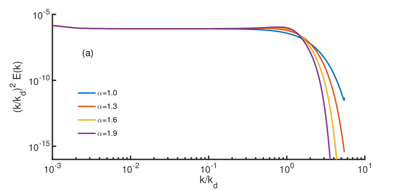
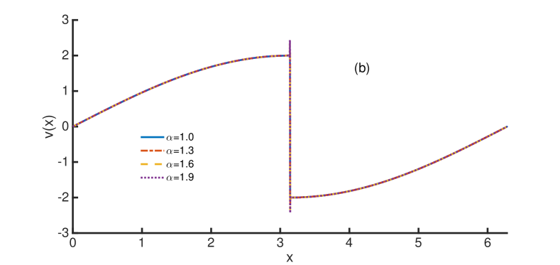
Figure 1: Results of direct numerical simulations of the Burgers equation with hyperviscosity such that $\alpha\in[1,2]$. In (a) we plot the compensated energy spectra i.e. $(k/k_{d})^{2}E(k)$ versus $k/k_{d}$ and in (b) we plot the velocity field structure in real space.

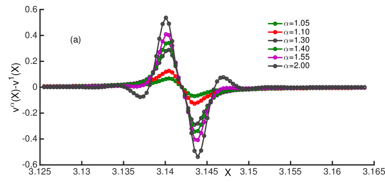
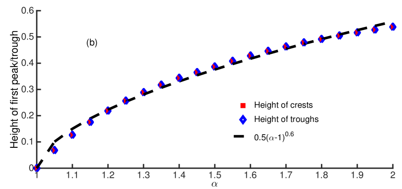
Figure 2: Detailed exploration of the shock structure gives us the above details. In (a) we plot the magnitude of discrepancy between the solutions of the hyperviscous Burgers and the viscous Burgers equations ($|v^{\alpha}(x)-v^{1}(x)|$ vs. $x$) keeping all other parameters like time of measurement, initial amplitude, and value of the coefficient of hyper viscosity same. In (b) we show how the absolute value of the peak or trough increases as we go from the limit of $\alpha=1$ to $\alpha=2$. The dashed line in (b) is obtained by fitting the data.

In Fig. 1(a) we see the compensated energy spectrum of the solutions of Eq. (1) and the corresponding flow structure in real space is given in Fig. 1(b). The $k^{-2}$ spectrum arises from the Fourier transform of the real space shock structure. The functional from of the shock structure that we see in the Fig. 1(b) can be calculated by solving the Eq. (1) using methods from boundary layer techniques at the steady state. In this method we consider the outer solution and the inner solution of the equation. The outer solution gives the large scale behaviour determined by the large scale forcing and setting viscous term to zero. While the inner solution corresponds to the effect of viscous term at the shock front. The oscillations that we see straddling the shock front, particularly visible on zooming at the shock front in Fig. 2 (a), is generated by the effect of the hyperviscosity. Clearly, the viscous ($\alpha=1$) limit shows no oscillations and hence no bottlenecks while for hyperviscosity ($\alpha>1$) we see the oscillations emanating out of the solutions of Eq. (1). The analytical solutions that we can calculate for the integral-hyperviscous cases do not work for the fractional hyperviscous case but one can still study these cases via simulations using pseudo-spectral method.

In Fig. 2 (a) we show how the amplitude of oscillations grow with increasing $\alpha$. The amplitude of the first visible peak versus $\alpha$ is fitted using a functional form $a_{1}(\alpha-1)^{a_{2}}$, where $a_{1}$ and $a_{2}$ are the fitting parameters. The fitted function is plotted with a black dashed line in Fig. 2 (b) we find that the fitted parameters are $a_{1}\sim 0.5$ and $a_{2}\sim 0.6$. The oscillation amplitude has a critical behaviour at $\alpha=1$ For values of $\alpha$ even fractionally larger than 1 we see the oscillations developing at the shock front while for $\alpha\leq 1$ no such oscillations develop at the shock front. We later show that this critical behaviour is due to the presence of singularity leading to non analytic behaviour. However, it must be noted that reduction of $\alpha$ cannot be continued too much below 1 as there is another critical point at $\alpha=0.5$  Bardos1979 ; Miao2009 .

3.2 Asymptotic method

The real space structure that we get from the numerical simulations can also be obtained by solving Eq. (1) using matched asymptotes. We need to essentially match the solutions of the equation obtained at the outer limit and the inner limit. The first step to solving the equations is to set $\partial_{t}v=0$ at the steady state. Now, we are left with an ordinary differential equation. Next, we consider the outer limit of the solution and then the inner limit of the solution and a simple matching would give the complete solution of the equations. To obtain the outer solution, which corresponds to the large scale behaviour and is unaffected by hyperviscosity, we set $\nu_{\alpha}^{\rm eff}=0$ and hence obtain the equation:

$$\frac{\partial}{\partial x}v^{2}(x)=2\sin(x).$$ (2)

On solving the above equation we get $v(x)=2{\rm sgn}(x-\pi)\sin(x/2)$. Where $x=\pi$ gives the location of the shock for the forcing used.

The inner solution which essentially gives the inner structure of the shock due to the effect of the viscous term can be obtained by first rescaling $X=(x-\pi)/\nu_{\alpha}^{\beta}$, where $\beta=1/(2\alpha-1)$ and then expanding the velocity in powers of $\nu_{\alpha}^{\rm eff}$. We then assume the limit $\nu_{\alpha}^{\rm eff}\rightarrow 0$ and retain the leading order term. This leads to the inner equation:

$$\frac{d}{dX}v^{2}(X)=-2(-1)^{-\alpha}\frac{d^{2\alpha}}{dX^{2\alpha}}v(X)$$ (3)

The above equations need to solved using boundary conditions that are a consequence of the outer solution discussed in the previous paragraph which is $v(\pm\infty)=\mp 2$. Now, considering the $\alpha=1$ case we are left with:

$$\frac{d}{dX}v(X)=\frac{1}{2}(v^{2}(X)-4),$$ (4)

on solving we get $v(X)=-2\tanh(X)$. For the hyperviscous case of $\alpha=2$ the solution is a bit more tricky to get and we need to consider the linear disturbances from a zeroth order shock solution. To do so we write $v(X)=-2+w(X)$, for $X>0$ and retain terms linear in $w(X)$. This gives us a linear ordinary differential equation in $w(X)$ where $w(X)$ is the linear disturbance, hence we have:

$$\frac{d^{3}}{dX^{3}}w(X)=2w(X)$$ (5)

To solve the above equation we consider solutions of type $e^{\mu X}$ and plug it in the above equation this gives us the algebraic equation $\mu^{3}-2=0$. Now, $\mu$ has a real solution and a pair of complex conjugate solutions. The complex solutions for $\mu$ gives us oscillatory behaviour which characterises the oscillations straddling the shock and hence leading to bottlenecks in energy spectrum. For $\alpha=1+\varepsilon$ we need to use techniques of fractional calculus to solve the equation for fractional $\varepsilon$. Interestingly though, there is an intermediate $\alpha=3/2$ where the differential equation is non-fractional:

$$\frac{d^{2}}{dX^{2}}w(X)=-2iw(X)$$ (6)

The solution of this equation gives oscillatory solutions like that of the higher integral order $\alpha$ cases. At this stage let us quickly review the solutions for $\varepsilon=0$ in the normal $x$- coordinate. From matching the inner and outer solution we get $v(x)=-2\tanh(x/2\nu_{\alpha}^{\rm eff})\sin(x/2)$. The $\tanh$–function leads to a spectrum with a scaling $|\hat{v}(k)|\sim 1/k$ in the limit of $\nu_{\alpha}^{\rm eff}\rightarrow 0$.

3.3 Fractional derivatives

In the previous two subsections we have been able to understand using numerical simulations and asymptotic methods the presence of oscillations around the shock for hyperviscous burgers equation with integer order of hyperviscosity and also the case of non-interger hyperviscosity with order $\alpha=3/2$, where the differential equation reduces to a non-fractional differential equation. To understand how fractional derivatives lead to the growth of oscillatory behaviour in the shock front let us start by looking at the linear equation for the disturbance from a shock solution. Thus we start with:

$$-(-1)^{-\alpha}\frac{d^{2\alpha-1}}{dX^{2\alpha-1}}w(X)=2w(X).$$ (7)

Now, we rewrite the above equation as and discuss the regime where $\alpha\in[1,2]$:

$$\frac{d^{\gamma}}{dX^{\gamma}}w(X)=-2e^{i\pi\alpha}w(X),$$ (8)

where, $\gamma=2\alpha-1$. Now we use the properties of fractional derivatives as discussed in the Appendix to rewrite the differential equation as:

$$\frac{d^{\gamma}}{dX^{\gamma}}\left(w(X)-\Sigma_{k=0}^{m-1}\frac{c_{k}t^{k}}{k!}\right)=-2e^{i\pi\alpha}w(X).$$ (9)

here, $m-1$ is the integer part of $\gamma$. Using the above equation and the Laplace transform method discussed in Appendix we obtain the solutions in terms of complex integrals as shown below:

$$w(X)=\frac{1}{2\pi i}\int_{Br}e^{sx}\frac{s^{\gamma}}{s^{\gamma}+e^{i\pi\alpha}}ds$$ (10)

Where we are integrating along the Bromowich path which is $Re(s)=\sigma$. Also the solution can be divided into two parts: $w(x)=w_{0}(x)+w_{1}(x)$. The first part $w_{0}(x)$ consist of the integration along the outer contour; i.e.:

$$w_{0}(x)=\frac{1}{2\pi i}\int_{Ha(\epsilon)}e^{sx}\frac{s^{\gamma}}{s^{\gamma}+e^{i\pi\alpha}}ds$$ (11)

and the second part $w_{1}(x)$ consist of the residues at the poles present in the main Reimann sheet which implies:

$$w_{1}(x)=\Sigma_{h}e^{s_{h}^{\prime}x}Res\left[\frac{s^{\gamma}}{s^{\gamma}+e^{i\pi\alpha}}\right]$$ (12)

Now imposing the condition that the pole has to be present in the first Reimann sheet gives us the following relation:

$$\left|\frac{\pi\alpha}{2\alpha-1}\right|<\pi$$ (13)

Clearly from the above inequality we can see that for $\alpha>1$ there is a pole in the physical Reimann sheet and for $\alpha\leq 1$ this pole is not present in the physical Reimann sheet. This absence of the pole singularity leads to an absence of oscillations in the physical velocity field for $\alpha\leq 1$.

4 Summary and conclusions

Shock front oscillations and as a consequence bottlenecks are generated in the Burgers equation by hyperviscosity even if it is present to a very low order. For integral order of hyperviscosity asymptotic methods have been employed to show the presence of these oscillations but for fractional order of hyperviscosity the verification is possible only by direct numerical simulations. In this paper we consider fractional order of hyperviscosity between normal viscosity and the lowest order of hyperviscosity to see the development of bottlenecks for small orders of hyperviscosity. We find that unlike the crossover between dissipative hyperviscous to conservative burgers the normal viscosity behaves like a critical point for the existence of bottlenecks.

Simplified hydrodynamic equations like the Burgers equation form a key basis for understanding a more complicated problem of fluid turbulence. The work presented in this paper would open questions more pertinent to the problem of fluid turbulence as a physical problem and the Navier-Stokes equation as a mathematical problem. One of the most important questions that arise now is related to fact that bottlenecks form in normal viscous Navier-Stokes turbulence but is it possible to have some fractional $\alpha<1$ such that there is a transition to a no-bottleneck spectra ? It remains to be investigated using high resolution direct numerical simulations of Navier-Stokes equation. Also the next question that would arise is whether such a transition is critical like the case of Burgers equation.

Hyperviscosity has been used quite commonly in research papers studying turbulence in fluids and plasmas Pandit2017 ; BanerjeeMHD2014 ; BanerjeeMHD2019 using both direct numerical simulations and shell models. The use of hyperviscosity becomes absolutely essential for certain class of equations like the Hall MHD BanerjeeHMHD2013 equations where the non linearity has different dominant behaviour for smaller length scales. The presence of fractional hyperviscosity in Hall MHD equations can be an important problem to investigate. Fractional diffusion has been used as an important way to model diffusion in polymer solutions and the signature of complex singularities on real space structures may even be probed experimentally.

5 Acknowledgements

DB would like to thank U. Frisch, R. Pandit, S. S. Ray, and W. Pauls for discussions and COST Action MP 1305 for support.

6 Appendix

In this appendix we show how we solve the fraction differential equations discussed in the results section.

Let us consider the fractional differential equation as discussed in the paper:

$$\frac{d^{\gamma}}{dX^{\gamma}}w(X)=-2e^{i\pi\alpha}w(X).$$ (14)

Let us also define operators $D^{\gamma}$ and $J^{\gamma}$ such that $D^{\gamma}$ is a fractional differential operator and $J^{\gamma}$ is a fractional integral operator. Amongst the various properties of these operators what is very useful for us here is the property that $D^{\gamma}J^{\gamma}={\bf I}$ but $J^{\gamma}D^{\gamma}\neq{\bf I}$. The detailed explanation can be found in the literature for example in Ref. Gorenflo .

The above differential equation can therefore be written as:

$$D^{\gamma}\left(w(X)-\Sigma_{k=0}^{m-1}\frac{c_{k}X^{k}}{k!}\right)=-2e^{i\pi\alpha}w(X)$$ (15)

On applying the operator $J^{\gamma}$ and taking the Laplace transform we get:

$$\tilde{w}(s)=\Sigma_{k=0}^{m-1}\frac{c_{k}}{s^{k+1}}-2e^{i\pi\alpha}\frac{1}{s^{\gamma}}\tilde{w}(s),$$ (16)

which in turn gives us:

$$\tilde{w}(s)=\Sigma_{k=0}^{m-1}c_{k}\frac{s^{\gamma-k-1}}{s^{\gamma}+e^{i\pi\alpha}}.$$ (17)

To obtain $w(X)$ we need to take a Laplace transform of the above expression $\tilde{w}(s)$. In this Laplace transform integral, for a pole type singularity to occur we need $s=e^{-i(2h+1)\pi\alpha/\gamma}$, with integer $h$. Now the phase in the exponential lies in the principle Reimann sheet when $|\pi\alpha/2\alpha-1|<\pi$. This happens only for $\alpha>1$.

References

- (1) Y. Kaneda, T. Ishihara, M. Yokokawa, K. Itakura, and A. Uno. Phys. of Fluids 15, L21 (2003).
- (2) W. Dobler, N. Erland, L. Haugen, T. A. Yousef, and A. Brandenburg. Phys. Rev. E 68, 026304 (2003).
- (3) A. Beresnyak. Phys. Rev. Lett. 106, 075001 (2011).
- (4) D. Donzis and K. R. Sreenivasan, J. Fluid Mech. 657, 171 (2010).
- (5) A.N. Kolmogorov, Dokl. Akad. Nauk. SSSR 30, 299303 (1941).
- (6) U. Frisch Turbulence : The legacy of A. N. Kolmogorov, (Cambridge University Press, Cambridge, UK, 1995).
- (7) G. Falkovich. Physics of Fluids 6, 1411 (1994).
- (8) U. Frisch, S. S. Ray, G. Sahoo, D. Banerjee, and R. Pandit. Phys. Rev. Lett. 110, 064501 (2013).
- (9) J. M. Burgers Advances in Appl. Mech. 1 171-199 (1948).
- (10) J. Bec and K. Khanin Physics Reports 447, Issues 1–2, 1-66 (2007).
- (11) J. Bec, J, R. Iturriaga, and K. Khanin. Phys. Rev. Lett. 89, 024501 (2002).
- (12) U. Frisch and J. Bec, Burgulence. In: Lesieur M., Yaglom A., David F. (eds) New trends in turbulence Turbulence: nouveaux aspects. Les Houches - Ecole d’Ete de Physique Theorique, 74 Springer, Berlin, Heidelberg (2002).
- (13) U. Frisch, S. Kurien, R. Pandit, W. Pauls, S. S. Ray, A. Wirth, and J.-Z. Zhu. Phys. Rev. Lett. 101, 144501 (2008).
- (14) D. Banerjee and S. S. Ray. Phys. Rev. E 90, 041001(R) (2014).
- (15) N. Erland, L. Haugen, and A. Brandenburg Phys. Rev. E 70, 026405 (2004).
- (16) C. Cichowlas, P. Bonaïti, F. Debbasch, and M. Brachet. Phys. Rev. Lett. bf 95, 264502 (2005).
- (17) S. S. Ray, U. Frisch, S. Nazarenko, and T. Matsumoto Phys. Rev. E 84, 016301 (2011).
- (18) S. S. Ray Pramana 84 (3), 395-407 (2015).
- (19) S. Thalabard and B. Turkington Journal of Physics A: Mathematical and Theoretical, 49, Number 16 (2016).
- (20) P. Fenga, J. Zhang, S. Cao, S. V. Prants, and Y. Liu Communications in Nonlinear Science and Numerical Simulation 45 104-116 (2017).
- (21) V. Shukla, M. Brachet, and R. Pandit New Journal of Physics, 15, (2013).
- (22) F. Mainardi Chaos, Solitons and Fractals 7, Issue 9, 1461-1477 (1996).
- (23) C. Bardos, P. Penel, U. Frisch, and P. L. Sulem Arch. Rational Mech. Anal. 71 (3), 237–256 (1979).
- (24) C. Miao and G. Wu J. Differential Equations 247, 1673–1693 (2009).
- (25) R. Pandit et. al. Phys. Fluids 29 (11) 111112 (2017).
- (26) D. Banerjee and R. Pandit Phys. Rev. E 90 0130018 (2014).
- (27) D. Banerjee and R. Pandit Phys. Fluids 31 (6) 065111 (2019).
- (28) D. Banerjee, S.S. Ray, G. Sahoo, and R. Pandit Phys. Rev. Lett. 111 (17) 174501 (2013).
- (29) FRACTIONAL CALCULUS : Integral and Differential equations of Fractional order. R. Gorenflo and F. Mainardi.