Oscillations of coronal loops using Rayleigh-Ritz technique

Abstract

In this paper, we apply the Rayleigh-Ritz Variational Scheme for studying the transverse oscillations of a magnetic flux tube. The flux tube is considered in low-$\beta$ solar coronal condition. The perturbations decomposed into irrotational and solenoidal components and MHD equations are reduced as a matrix eigenvalue problem. In the case of longitudinally stratified thin flux tube, the fundamental and higher order kink frequencies are computed. The results are in good agreements with previous studies.

1 Introduction

An understanding of the nature and propagation of waves in magnetic structures is of considerable interest, especially as flux tubes are important in the heating of stellar and solar chromosphere and corona. The observational ability of spacecrafts such as Yohkoh, SoHO, and TRACE provided us with detections of coronal waves (e.g., Aschwanden et al. 1999; Nakariakov et al. 1999; Wang et al. 2003; Wang & Solanki 2004; Berghmans & Clette 1999; De Moortel et al. 2000). Direct observations of fundamental quantities such as the magnetic field strength of solar corona is still difficult (Verth & Erdélyi 2008; Ruderman et al. 2008; Van Doorsselaere et al. 2008). However, the coronal and magneto seismology techniques allow the information to be extracted from observations of oscillatory phenomena and the results to be interpreted using theoretical models (Roberts et al. 1984; Goossens et al. 1992).

Several theoretical models of coronal loops have been developed. The earlier models considered the simple aspects of magnetic flux tubes (e.g. Edwin & Roberts 1983). In their slab and cylindrical flux tube models, infinitely long and straight uniform magnetic field, plasma density of loop comparable with its environment, constant cross section, constant gravitation, isothermal structure, and no initial flow, were considered.

In the recent observational data, periods, phases, damping times, and mode profiles for coronal loops are reported by Verwichte et al. 2004; De Moortel & Brady 2007. As expected, the results differ from those based on simplified theoretical models. To be more realistic several features may be added to this simple model, such as the presence of magnetic twist and shells (Bennett et al. 1999; Sakai et al. 2000; Erdélyi & Fedun 2006; Erdélyi & Carter 2006; Ruderman 2007), or field-aligned flows (Terra-Homem et al. 2003), the role of line-tying effects (Díaz et al. 2004), loop curvature (Smith et al. 1997; Van Doorsselaere et al. 2004; Brady & Arber 2005), coronal leakage (Díaz et al. 2004; Brady & Arber 2005).

Oscillations of longitudinally density stratified coronal loops are investigated by Mendoza-Briceńo et al. 2004; Andries et al. 2005a, b; Donnelly et al. 2006; Roberts 2006; Karami & Asvar 2007; Safari et al. 2007; Andries et al. 2009; Pascoe et al. 2009. The effect of elliptical cross-section on loop oscillations is studied by Ruderman 2003. Oscillations of multistranded loops are discussed by Luna et al. 2009. See Aschwanden (2004, 2009) and Nakariakov & Verwichte (2005) for an extended review of observations of coronal oscillations.

Despite the extensive work there are still many aspects of coronal loop oscillations and coronal seismology to be explored. But the previous methods, mostly based on solving differential equations, have those own complications and inconveniences. Avoiding complications of differential equations, a Rayleigh-Ritz variational method can be developed. Sobouti (1981) used a Rayleigh-Ritz variational scheme to define p- and g-modes of self-gravitating fluids. He used a gauged version of Helmholtz’s theorem to decompose the perturbations into an irrotational and a solenoidal components, which was further splitted into the sum of poloidal and toroidal components. These components were related to p-, g- and toroidal modes of fluid. Hasan & Sobouti (1987; henceforth referred to as HS) treated the wave propagation in a uniform magnetic flux tube with a rectangular cross-section and solid boundary conditions (trapped modes). Nasiri (1992) extended the analysis of HS to include a variable cross section with vertical non-uniform magnetic filed.

Here, we investigated HS analysis to study the transverse oscillations of a longitudinally density stratified coronal loop. Equations of motion, and decomposition of Lagrangian displacements are dealt with in Sects. 2 & 3. The possible motions in a cylindrical flux tube are treated in Sec 4. The numerical results and conclusions are given in Sect. 5.

2 Equations of motion

The linearized MHD equations for the Eulerian perturbations of a fluid with equilibrium values of density $\rho_{0}$, gravity acceleration $g_{0}$, pressure $p_{0}$, and magnetic filed $\textbf{B}_{0}$ are

$$\rho_{0}\frac{\partial^{2}\xi}{\partial t^{2}}=-\textbf{F}(\xi),$$ (1)

where

$$\textbf{F}(\xi)=\nabla p-\rho\textbf{g}_{0}-\frac{1}{4\pi}(\nabla\times\textbf{b})\times\textbf{B}_{0},$$ (2)

$$\rho=-\rho_{0}\nabla\cdot\xi-\xi\cdot\nabla\rho_{0},$$ (3)

$$p=-\gamma p_{0}\nabla\cdot\xi-\xi\cdot\nabla p_{0},$$ (4)

$$\textbf{b}=\nabla\times(\xi\xi\times B_{0}),~{}~{}\textbf{v}=\frac{\partial\xi\xi}{\partial t},$$ (5)

in which $p$, $\rho$ and b are the perturbations of pressure, density and magnetic field, respectively. $\xi\xi({\bf x},t)$ denote a small Lagrangian displacement of fluid element from its equilibrium position. The perturbation of gravity is neglected.

On multiplying Eq. (1) by $\xi\xi^{*}$ and integrating over the volume initially occupied by the flux tube, one obtains

$$\!\!\!\!\omega^{2}\int{d\textbf{x}\xi\xi^{*}.\rho_{0}\xi\xi}=\int{d\textbf{x}\xi\xi^{*}\cdot\textbf{F}(\xi\xi)}$$ (6)

$$\!\!\!\!=\int{d\textbf{x}[\xi\xi^{*}\cdot\nabla p-\xi\xi^{*}\cdot\textbf{g}_{0}\rho-\frac{1}{4\pi}\xi\xi^{*}\cdot(\nabla\times\textbf{b})\times\textbf{B}_{0}]},$$

where, $\xi\xi(\textbf{x},t)$ is assumed to have a time dependence proportional to $\exp(i\omega t)$. HS have shown that, Eq. (6) can be reduced as

$$w-\omega^{2}s \!\!\!\!=0,$$ (7)

where

$$s= \!\!\!\!\int{d\textbf{x}\rho_{0}\xi\xi^{*}\cdot\xi\xi},$$ (8)

$$w= \!\!\!\!\int{d\textbf{x}\frac{1}{\rho_{0}}\frac{dp_{0}}{d\rho_{0}}\rho^{*}\rho}$$

$$\!\!\!\!+\int{d\textbf{x}\Gamma p_{0}\nabla\cdot\xi\xi^{*}\nabla\cdot\xi\xi}+\frac{1}{4\pi}\int{d\textbf{x}\textbf{b}^{*}\cdot\textbf{b}},$$

in which $\Gamma=\gamma-(p/\rho)(dp/d\rho)$. From Eq. (8), $s$ is symmetric and positive definite ($\rho_{0}>0$). Therefore, we may write $\omega^{2}=w/s$. From Eq. (2), the first term of $w$ is symmetric and positive ($dp_{0}/d\rho_{0}>0$). It can be zero if and only if $\rho=0$, which is possible if $\rho_{0}\xi\xi$ is solenoidal. The second term of $w$ is symmetric and positive for convectively stable fluids, i.e. when $\Gamma>0$. It is zero for convectively neutral fluids ($\Gamma=0$) and also for solenoidal motions($\nabla\cdot\xi\xi=0$). For convectively unstable fluids ($\Gamma<0$), the second term of $w$ contributes negatively. Thus, the contribution of this term to $\omega^{2}$ maybe positive, zero or negative. The last term of $w$ is symmetric and positive too, unless $b=0$, whenever it vanishes. Therefore, this term also contributes positively to $\omega^{2}$. The sum $w$ is symmetric, thus ruling out either damping or overstability. There is, however, the possibility of dynamical instability if the fluid is convectively unstable. $w$ is composed of three separated terms, with distinct nature. The first, second and third terms indicate the pressure, buoyancy and magnetic forces, respectively. Equation (1) or its equivalent variational form, Eq. (7), constitute a generalized eigenvalue problem.

2.1 Boundary Conditions

We consider a general flux tube with its ends on the dense plasma as shown in Fig 1. In the figure, ${\bf n_{1}}$, ${\bf n_{2}}$, and ${\bf n_{3}}$ are the normal vectors to the lateral surface $S_{1}$, and two end surfaces $S_{2}$ and $S_{3}$, respectively. The flux coordinates, $(q_{1},q_{2},q_{3})$, are adopted as shown in the Fig. 1. We assume the hydrostatic equilibrium set of temperature, density, gas pressure, and magnetic field, $(T_{0i},\rho_{0i},P_{0i},{\bf B_{0i}})$ for interior, and $(T_{0e},\rho_{0e},P_{0e},{\bf B_{0e}})$ for exterior regions of the flux tube with an adiabatic process. The background magnetic field is potential field and the initial material flow and the dissipative terms are neglected. The gravity, ${\bf g_{0}}$, is constant.

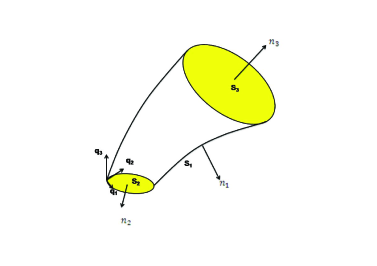
Figure 1: A sketch of the equilibrium model of the flux tube. ${\bf n_{1}}$, ${\bf n_{2}}$, and ${\bf n_{3}}$ are the normal vectors to the lateral surface $S_{1}$, two end surfaces $S_{2}$ and $S_{3}$, respectively.

The boundary conditions for tube surfaces which are parallel to the equilibrium magnetic field are given as

$$\hat{n_{1}}\cdot[{\bf v}]=\hat{n_{1}}\cdot[{\bf b}]=0,~{}~{}[P_{T}]=0,$$ (10)

where $\hat{n_{1}}$ is the normal unit vector to the lateral surface, $P_{T}=p+\frac{B^{2}}{8\pi}$, and $[f]=f_{\rm interior}-f_{\rm exterior}$. For two ends of the flux tube, the boundary conditions are

$${\bf v}.\hat{n}_{2,3}={\bf b}.\hat{n}_{2,3}=P_{T}=0.$$ (11)

in which $\hat{n_{2}}$ and $\hat{n_{3}}$ are the normal unit vectors to the end surfaces. See also Donnelly et al. (2006) and references therein for more details.

3 Decomposition of Lagrangian displacements

Let $\zeta\zeta(\textbf{x},t)$ denote a linear displacement in the fluid. The collection of all such displacements will belong to a Hilbert space $\cal{H}$. We define the inner product in $\cal{H}$ of $\zeta\zeta$ and $\zeta\zeta^{\prime}$ as

$$(\zeta\zeta,\zeta\zeta^{\prime})=\int{d\textbf{x}\rho\zeta\zeta^{*}\cdot\zeta\zeta^{\prime}};~{}~{}~{}\zeta\zeta,\zeta\zeta^{\prime}\epsilon\cal{H}.$$ (12)

By a suitable gauge transformation, $\zeta\zeta$ can be decomposed using Helmholtz’s theorem as follows (see Sobouti (1981))

$$\zeta\zeta=\zeta\zeta_{1}+\zeta\zeta_{2}+\zeta\zeta_{3},$$ (13)

where the various components can be expressed in terms of scalar functions $\chi_{1}$, $\chi_{2}$, and $\chi_{3}$

$$\!\!\!\!\zeta\zeta_{1}=-\nabla\chi_{1},~{}~{}(\rm{irrotational}),$$ (14)

$$\!\!\!\!\zeta\zeta_{2}=\nabla\times\nabla\times(\hat{q_{3}}\chi_{2}),~{}~{}(\rm{toroidal}),$$ (15)

$$\!\!\!\!\zeta\zeta_{3}=\nabla\times\nabla\times\nabla\times(\hat{q_{3}}\chi_{3}),~{}~{}(\rm{poloidal}).~{}$$ (16)

It can be shown that, the decomposition is complete, however, not unique. Let $\{\xi\xi_{l};l=1,2,3\}$ be an eigenvector of Eq. (1). Consider $\{\zeta\zeta_{s};s=1,2,3\}=\{\zeta\zeta_{1i},\zeta\zeta_{2j},\zeta\zeta_{3k};i,j,k=1,2,...\}$ as a complete set of basis vectors in the Hilbert space of the displacement vectors that satisfies equations of motion. Expanding $\xi\xi_{l}$ in terms of $\{\zeta\zeta_{s}\}$, one gets

$$\xi\xi_{l}=\sum_{s}\zeta\zeta_{s}Z_{sl},$$ (17)

where $Z_{sl}$ are proportionality constants. Substituting Eq. (17) into Eqs (7)-(2) and using a variational technique to minimize the eigenvalue, gives the following matrix equation

$$\textbf{W}\textbf{Z}=\textbf{S}\textbf{Z}\textbf{E},$$ (18)

where E is a diagonal matrix whose elements are the eigenvalues $\omega_{l}$ and $\textbf{Z}=[Z_{ls}];$ $l,s=1,2,3$, is the matrix of the expansion coefficients. The functional expressions for the elements of W and S are the same as of Eqs (8) and (2) with $\xi\xi$ replaced by $\zeta\zeta_{s}$. The functional forms used for $\zeta\zeta_{s}$, for different three displacements are given in A.

3.1 Block structure of the S, W, E and Z matrices

Schematically, the blocks of S have following structure

$$\textbf{S}=\pmatrix{S_{11}&S_{12}&S_{13}\cr S_{21}&S_{22}&S_{23}\cr S_{31}&S_{32}&S_{33}}.$$ (19)

Explicit expressions for the block elements of S are given in B. The block structure of W matrix will be

$$\textbf{W}=\pmatrix{W_{11}&W_{12}&W_{13}\cr W_{21}&W_{22}&W_{23}\cr W_{31}&W_{32}&W_{33}}.$$ (20)

The blocks of $W_{23}$ and $W_{13}$ will be zero. Explicit expressions for the block elements of W are given in C. By definition, the matrix of eigenvalues is block diagonal,

$$\textbf{E}=\pmatrix{E_{11}&0&0\cr 0&E_{22}&0\cr 0&0&E_{33}},$$ (21)

where each block is itself a diagonal matrix. The matrix Z has a full structure, i.e., in general, all modes have components in all there subspaces. Thus, the Z matrix can schematically be written as

$$\textbf{Z}=\pmatrix{Z_{11}&Z_{12}&Z_{13}\cr Z_{21}&Z_{22}&Z_{23}\cr Z_{31}&Z_{32}&Z_{33}}.$$ (22)

3.2 Method of solution

In order to determine the frequencies, we need to solve Eq. (18), which was obtained from the original Eq. (7) by applying a variational principle. We adapt a Rayleigh-Ritz procedure and approximate the linear series in Eq. (18) by a finite number of terms, say $n$. The matrix blocks $S_{ls}$ and $W_{ls};l,s=1,2,3$ become $n\times n$ matrices.

4 The case of cylindrical flux tube

Let us consider a special circular cylinder model of coronal loop. The cylinder is considered with its ends at the photosphere and with a relatively small curvature (i.e., the radius of curvature of the loop is much larger than the loop length) to be pervaded by a uniform magnetic field along its axis, $B=B_{0}\hat{z}$, and to have low gas pressure (low-$\beta$ approximation) with isothermal equilibrium state. The length and radius of the loop are L and R, respectively. We adopt a cylindrical coordinates, (r, $\phi$, z) with the $z$ axis parallel to the magnetic field (the $\hat{q_{3}}$ axis in flux coordinate) and the origin at the center of one tube ends. The density is assumed to be

$$\rho(\epsilon,z)=\left\{\begin{array}[]{cc}\rho_{i}(\epsilon)f(\epsilon,z),&r\leq R,\\ \rho_{e}(\epsilon)f(\epsilon,z),&r\geq R,\end{array}\right.$$ (23)

$$f(\epsilon,z)=\exp{(-\frac{\epsilon}{\pi}\sin{\frac{\pi z}{L}}});~{}~{}\rho_{i,e}(\epsilon)=\frac{\rho_{i0,e0}}{\int^{L}_{0}{f(\epsilon,z)dz}},$$ (24)

where $\epsilon=L/H$ ($H$ is the density scale height) and $\rho_{i0}$ and $\rho_{e0}$ are the interior and exterior densities at the footpoints of the loop, respectively. The proposed trial functions for $\chi_{l}$, are considered as

$$\chi_{l(l=1,2,3)}=\left\{\begin{array}[]{cc}F_{i}(r)e^{im\phi}Z_{l}(z),&r\leq R,\\ {a_{mn}}F_{e}(r)e^{im\phi}Z_{l}(z),&r\geq R.\end{array}\right.$$ (25)

In the case of the body waves, $F_{i}(r)=J_{m}(\gamma_{mn}^{i}r)$, ${\gamma_{mn}^{i}}^{2}>0$, and the surface waves $F_{i}(r)=I_{m}(|\gamma_{mn}^{i}|r)$, ${\gamma_{mn}^{i}}^{2}<0$. For both body and surface waves, we consider the evanescent waves for exterior, $F_{e}(r)=K_{m}(\gamma_{mn}^{e}r)$, ${\gamma_{mn}^{e}}^{2}<0$. In above formula, $\gamma_{mn}^{\rm i}$ and $\gamma_{mn}^{\rm e}$ are the radial wave numbers for interior and exterior, respectively.

To satisfy Eqs. (10) and (11), $Z_{l}(z)$ functions are chosen as

$$\begin{array}[]{cc}Z_{1}(z)=\cos{kz},\\ Z_{2}(z)=\sin{kz},\\ Z_{3}(z)=\sin{kz}.\end{array}\\ ~{}~{}k=\frac{n\pi}{L},\\ ~{}~{}0<z<L$$ (26)

Using Eqs. (13)-(16), (25), and (26), and imposing boundary conditions (10) and (11) we obtain

$$\frac{1}{\gamma_{mn}^{i}}\frac{J^{\prime}_{m}(\gamma_{mn}^{i}R)}{J_{m}(\gamma_{mn}^{i}R)}=\frac{1}{\gamma_{mn}^{e}}\frac{K^{\prime}_{m}(\gamma_{mn}^{e}R)}{K_{m}(\gamma_{mn}^{e}R)},$$ (27)

$$a_{mn}=-\frac{{B_{0}^{2}}_{i}}{{B_{0}^{2}}_{e}}\frac{J_{m}(\gamma_{mn}^{i}R)}{K_{m}(\gamma_{mn}^{e}R)}=-\frac{{B_{0}^{2}}_{i}}{{B_{0}^{2}}_{e}}\frac{J^{\prime}_{m}(\gamma_{mn}^{i}R)}{K^{\prime}_{m}(\gamma_{mn}^{e}R)},$$ (28)

where $J^{\prime}_{m}(x)$ is $dJ_{m}(x)/dx$. In thin tube approximation, $|\gamma_{mn}^{i,e}|R\ll 1$, Eq. (27) leads to ${\gamma_{mn}^{i}}^{2}={\gamma_{mn}^{e}}^{2}$.

5 Results and Conclusions

5.1 Results

As typical parameters for a coronal loop, we assume $\eta$ $(=R/L)=0.01$ for the ratio of radius to length, $\rho_{e}/\rho_{i}=0.1$ for the ratio of interior to exterior domain of density, $B_{i}/B_{e}=0.98$ for the ratio of interior to exterior domain of magnetic field (Aschwanden 2004). The $\beta$ parameters are $0.035$ and $0.00035$ for the loop interior and exterior, respectively.

Applying a numerical code, Eq. (18) is solved for eigenvalues and eigenfunctions. For unstratified loop ($\epsilon=0$), the frequencies have been calculated and plotted versus longitudinal mode numbers $n$ in Fig. 2. As expected, $\omega_{n}$ is proportional to its mode number (i.e., $\omega_{n}\approx n\omega_{1}$). For stratified loops, in a range of $0\leq\epsilon<20$, we have calculated the fundamental, first, second, and the third overtone kink ($m=1$) frequencies $\omega_{1}$, $\omega_{2}$, $\omega_{3}$, and $\omega_{4}$, respectively. The frequencies and their ratios are plotted in Fig. 3. As anticipated from the behavior of $f(\epsilon,z)$, all of the frequencies show monotonic increase with increasing $\epsilon$. As shown in the figure, for small $\epsilon$, the odd modes ($\omega_{1}$ and $\omega_{3}$) has steeper slopes than the even modes ($\omega_{2}$ and $\omega_{4}$), but modes successively approach each other as $\epsilon$ increases. The ratios $\omega_{n}/\omega_{1}$ ($n=2,3,4$) begins from $n$ for unstratified loops, $\epsilon=0$, and decreases as $\epsilon$ increases. This result is in agreement with Safari et al. (2007). From the TRACE data, Verwichte et al. (2004) find the ratio of the fundamental period to the first overtone to be $1.64$ and $1.81$ for two of their observed loops. Van Doorsselaere et al. (2007) revisited the same ratios from the observational data to be $1.58$ and $1.82$ for the same loops, respectively, and $1.795$ for another loop in their current analysis. From Fig. 3., corresponding values of $\epsilon$ are $7.44$ and $3.69$. Therefore, if we suppose typical loop lengths, $L=100$ and $400Mm$, then the density scale heights($H$) fall in the range of $H=\epsilon^{-1}L\simeq$ [13, 53] and [27, 108] Mm, respectively. As you see, the ratio of the fundamental period to the second starts from 3 and to the third start from 4. We should note that, due to variational methods, the lower frequencies are more precise and reliable. But their total treatment is in agreement with previous works.

From the observation, we know that $\eta$ differs from 0.01 to 0.04 (e.g. Goossens et al. 2002). Applying this variation on the model, the frequencies show a little increase. The result are shown in Fig. 4 for two corresponding values of $\epsilon$.

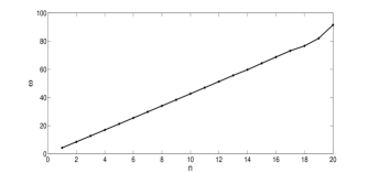
Figure 2: The frequencies for unstratified loop ($\epsilon=0$) versus longitudinal mode number, $n$. All frequencies are in units of $\pi v_{{A}_{i}}(\epsilon=0)/L$.

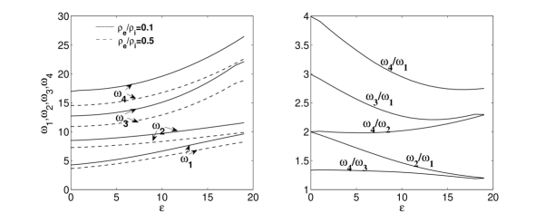
Figure 3: Fundamental, first, second, and third overtone frequencies versus $\epsilon$. All frequencies are in units of $\pi v_{{A}_{i}}(\epsilon=0)/L$.

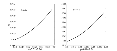
Figure 4: frequencies versus $\eta=R/L$, for $\epsilon=3.69$ and $7.44$. All frequencies are in units of $\pi v_{{A}_{i}}(\epsilon=0)/L$.

5.2 Conclusions

Still many open problems remain to be solved in the field of oscillations and real 3D structures of the coronal loops. Actually, the real structure of the magnetic filed, variable cross section or high $\beta$ plasmas, yet have not been modeled completely. The variational principles have already been applied to the problem of loop oscillations with regard to the simplified one-dimensional longitudinal kink equation obtained in the approximation of a ”thin tube”. However, Andries et al. (2009) pointed out recently that the variational principle may be used in a much more general sense involving integration in both spatial directions. This is exactly what Eq. (18) is about.

Here, the application of Rayleigh-Ritz variational method to study the transverse oscillation of a general configuration of magnetic flux tube has been investigated. As a special case, we study the oscillations of coronal loops with exponential density variations along the loop axis. The kink frequencies for unstratified loops, and the kink frequencies and the frequency ratios for stratified loops are found. Increasing the density contrast decreases the frequencies but their ratios and shape of the profiles remain unchanged. For typical loop lengths, $100-400$Mm, the density scale heights fall in the range of $13-108$Mm, in agreement with Andries et al. (2005a, b), Safari et al. (2007), McEwan et al. (2006), and Donnelly et al. (2006). The frequencies show a little increase as $\eta$ increases.

So despite the fact of complication of solving differential equations, the Rayleigh-Ritz variational method could go ahead in a definite and obvious process and reproduce the previous results.

Choosing the trial functions for each desired problem may be known as a challenge of this method. Having a suitable set of trial functions, this method could be extended to other studies of oscillations. In the case of this work, the trial functions have a simple forms but their selection is not so easy for more complicated geometries. The lack of suitable trial functions affects the convergency of the method, as well. In the case of zero external densities, like the investigation of internal oscillations of stars, the trial functions could be selected such that the calculations become more easy and the $S$ matrix becomes diagonal.

Another problem caused by variational method is missing the precision as one goes from the lower order modes to the higher ones. However, the results are satisfactory enough precise concerning the observational data in touch.

Acknowledgments: We would like to thank Prof. Y. Sobouti for his helpful comments through the work.

Appendix A Displacement vectors

Using Eqs. (14)-(16), (25) and (26) one gets

$$\zeta\zeta_{1}^{mn}=e^{im\phi}\left\{\begin{array}[]{cc}-\gamma_{mn}J^{\prime}_{m}(\gamma_{mn}r)\cos(kz)\hat{r}-\frac{im}{r}J_{m}(\gamma_{mn}r)\cos(kz)\hat{\phi}+kJ_{m}(\gamma_{mn}r)\sin(kz)\hat{z},&r\leq R,\\ {a_{mn}}(-\gamma_{mn}K^{\prime}_{m}(\gamma_{mn}r)\cos(kz)\hat{r}-\frac{im}{r}K_{m}(\gamma_{mn}r)\cos(kz)\hat{\phi}+kK_{m}(\gamma_{mn}r)\sin(kz)\hat{z}),&r\geq R,\\ \end{array}\right.$$ (31)

$$\zeta\zeta_{2}^{mn}=e^{im\phi}\left\{\begin{array}[]{cc}k\gamma_{mn}J^{\prime}_{m}(\gamma_{mn}r)\cos(kz)\hat{r}+\frac{ikm}{r}J_{m}(\gamma_{mn}r)\cos(kz)\hat{\phi}+\gamma^{2}J_{m}(\gamma_{mn}r)\sin(kz)\hat{z},&r\leq R,\\ {a_{mn}}(k\gamma_{mn}K^{\prime}_{m}(\gamma_{mn}r)\cos(kz)\hat{r}+\frac{imk}{r}K_{m}(\gamma_{mn}r)\cos(kz)\hat{\phi}+\gamma^{2}K_{m}(\gamma_{mn}r)\sin(kz)\hat{z}),&r\geq R,\\ \end{array}\right.$$ (34)

$$\zeta\zeta_{3}^{mn}=e^{im\phi}\left\{\begin{array}[]{cc}(\gamma_{mn}^{2}+(n\pi)^{2})[-\frac{im}{r}J_{m}(\gamma_{mn}r)\hat{r}+\gamma J^{\prime}_{m}(\gamma_{mn}r)\hat{\phi}]\sin(kz),&r\leq R,\\ {a_{mn}}((\gamma_{mn}^{2}+(n\pi)^{2})[-\frac{im}{r}K_{m}(\gamma_{mn}r)\hat{r}+\gamma K^{\prime}_{m}(\gamma_{mn}r)\hat{\phi}]\sin(kz)),&r\geq R.\\ \end{array}\right.$$ (37)

Appendix B Elements of S matrix

The elements of $S$ matrix are ($m=1$)

$$S_{11}^{nn^{\prime}} = 2\pi(\rho_{i}(\epsilon)\rm{fR1}+{a^{*}_{mn}}{a_{mn^{\prime}}}\rho_{i}(\epsilon)\rm{fR2})\times\rm{fZ1}$$ (38)

$$+2\pi(n\pi)(n^{\prime}\pi)(\rho_{i}(\epsilon)\rm{fR3}+{a^{*}_{mn}}{a_{mn^{\prime}}}\rho_{e}(\epsilon)\rm{fR4})\times\rm{fZ2},$$

$$S_{22}^{nn^{\prime}} = 2\pi(n\pi)(n^{\prime}\pi)(\rho_{i}(\epsilon)\rm{fR1}+{a^{*}_{mn}}{a_{mn^{\prime}}}\rho_{i}(\epsilon)\rm{fR2})\times\rm{fZ1}$$ (39)

$$+2\pi\gamma_{mn}^{2}\gamma_{mn^{\prime}}^{2}(\rho_{i}(\epsilon)\rm{fR3}+{a^{*}_{mn}}{a_{mn^{\prime}}}\rho_{e}(\epsilon)\rm{fR4})\times\rm{fZ2},$$

$$S_{33}^{nn^{\prime}} = 2\pi(\gamma_{mn}^{2}+(n\pi)^{2})(\gamma_{mn^{\prime}}^{2}+(n^{\prime}\pi)^{2})(\rho_{i}(\epsilon)\rm{fR1}$$ (40)

$$+{a^{*}_{mn}}{a_{mn^{\prime}}}\rho_{e}(\epsilon)\rm{fR2})\times\rm{fZ2},$$

$$S_{12}^{nn^{\prime}} = -\int{dS[\chi_{1}^{*}\rho\zeta\zeta_{2}\cdot\hat{n}]}+\int{d\textbf{x}\frac{d\rho}{dz}\chi_{1}^{*}{\zeta\zeta_{2}}_{z}}$$ (41)

$$= -2\pi n^{\prime}\pi(\rho_{i}(\epsilon)\rm{fR5}+{a^{*}_{mn}}{a_{mn^{\prime}}}\rho_{e}(\epsilon)\rm{fR6})\times\rm{fZ1}$$

$$+2\pi\gamma_{mn^{\prime}}^{2}(\rho_{i}(\epsilon)\rm{fR3}+a^{*}_{mn}{a_{mn^{\prime}}}\rho_{e}(\epsilon)\rm{fR4})\times\rm{fZ3},$$

$$S_{13}^{nn^{\prime}} = -\int{dS[\chi_{1}^{*}\rho\zeta\zeta_{3}\cdot\hat{n}]}$$ (42)

$$= 2\pi I(\gamma_{mn^{\prime}}^{2}+(n\pi)^{2})(\rho_{i}(\epsilon)\rm{fR7}+{a^{*}_{mn}}{a_{mn^{\prime}}}\rho_{e}(\epsilon)\rm{fR8})\times\rm{fZ4},$$

$$S_{23}^{nn^{\prime}} = \int{dS[\rho\frac{d\chi_{2}^{*}}{dz}\zeta\zeta_{3}\cdot\hat{n}]}$$ (43)

$$= -2\pi In\pi(\gamma_{mn^{\prime}}^{2}+(n\pi)^{2})(\rho_{i}(\epsilon)\rm{fR7}+{a^{*}_{mn}}{a_{mn^{\prime}}}\rho_{e}(\epsilon)\rm{fR8})\times\rm{fZ4},$$

in which

$$\rm{fR1} = \int_{0}^{1}{rdr(\frac{1}{2}\gamma_{mn}\gamma_{mn^{\prime}}[J_{m-1}(\gamma_{mn}r)J_{m-1}(\gamma_{mn^{\prime}}r)+J_{m+1}(\gamma_{mn}r)J_{m+1}(\gamma_{mn^{\prime}}r)])},$$

$$\rm{fR2} = \int_{1}^{\infty}{rdr(\frac{1}{2}\gamma_{mn}\gamma_{mn^{\prime}}[K_{m-1}(\gamma_{mn}r)K_{m-1}(\gamma_{mn^{\prime}}r)+K_{m+1}(\gamma_{mn}r)K_{m+1}(\gamma_{mn^{\prime}}r)])},$$

$$\rm{fR3} = \int_{0}^{1}{rdrJ_{m}(\gamma_{mn}r)J_{m}(\gamma_{mn^{\prime}}r)},$$

$$\rm{fR4} = \int_{1}^{\infty}{rdrK_{m}(\gamma_{mn}r)K_{m}(\gamma_{mn^{\prime}}r)}\},$$

$$\rm{fR5} = \frac{\gamma_{mn^{\prime}}}{2}J_{m}(\gamma_{mn}R)(J_{m-1}(\gamma_{mn^{\prime}}R)-J_{m+1}(\gamma_{mn^{\prime}}R)),$$

$$\rm{fR6} = \frac{\gamma_{mn^{\prime}}}{2}K_{m}(\gamma_{mn}R)(K_{m-1}(\gamma_{mn^{\prime}}R)+K_{m+1}(\gamma_{mn^{\prime}}R))],$$

$$\rm{fR7} = \frac{\gamma_{mn^{\prime}}}{2}J_{m}(\gamma_{mn}R)(J_{m+1}(\gamma_{mn^{\prime}}R)+J_{m-1}(\gamma_{mn^{\prime}}R)),$$

$$\rm{fR8} = \frac{\gamma_{mn^{\prime}}}{2}K_{m}(\gamma_{mn}R)(K_{m+1}(\gamma_{mn^{\prime}}R)-K_{m-1}(\gamma_{mn^{\prime}}R)),$$

$$\rm{fZ1} = \int^{1}_{0}{dzf(\epsilon,z)\cos{n\pi z}\cos{n^{\prime}\pi z}},$$

$$\rm{fZ2} = \int^{1}_{0}{dzf(\epsilon,z)\sin{n\pi z}\sin{n^{\prime}\pi z}},$$

$$\rm{fZ3} = \int^{1}_{0}{dz\frac{df(\epsilon,z)}{dz}\cos{n\pi z}\sin{n^{\prime}\pi z}},$$

$$\rm{fZ4} = \int^{1}_{0}{dzf(\epsilon,z)\cos{n\pi z}\sin{n^{\prime}\pi z}},$$

$$\rm{fZ5} = \int^{1}_{0}{dz\cos{n\pi z}\cos{n^{\prime}\pi z}},$$

$$\rm{fZ6} = \int^{1}_{0}{dz\sin{n\pi z}\sin{n^{\prime}\pi z}}.$$

Appendix C Elements of W matrix

Simplifying Eq. (2), the elements of $W$ matrix are

$$\frac{4\pi}{B_{0}^{2}}W_{ij} \!\!\!\!= \!\!\!\!(1+\frac{\Gamma\beta}{2})\int{d\bf{x}\nabla\cdot\zeta\zeta_{i}^{*}\nabla\cdot\zeta\zeta_{j}}-\int{d\bf{x}\frac{\partial\zeta\zeta_{zi}^{*}}{\partial z}\nabla\cdot\zeta\zeta_{j}}$$ (44)

$$\!\!\!\!-\int{d\bf{x}\nabla\cdot\zeta\zeta_{i}^{*}\frac{\partial\zeta\zeta_{zj}}{\partial z}}+\int{d\bf{x}\frac{\partial\zeta\zeta_{i}^{*}}{\partial z}\cdot\frac{\partial\zeta\zeta_{j}}{\partial z}},$$

$$\frac{2}{B_{0}^{2}}_{i}W_{11}^{nn^{\prime}} = (\gamma^{2}_{mn}+(n\pi)^{2})(\gamma^{2}_{mn^{\prime}}+(n^{\prime}\pi)^{2})$$ (45)

$$\{(1+\frac{\Gamma\beta_{i}}{2})\rm{fR3}+a^{*}_{mn}a_{mn^{\prime}}\frac{{B_{0}^{2}}_{e}}{{B_{0}^{2}}_{i}}(1+\frac{\Gamma\beta_{e}}{2})~{}\rm{fR4}\}\times\rm{fZ5}$$

$$+((n\pi)^{2}(n^{\prime}\pi)^{2}-(n\pi)^{2}(\gamma^{2}_{mn^{\prime}}+(n^{\prime}\pi)^{2})-(n^{\prime}\pi)^{2}(\gamma^{2}_{mn}+(n\pi)^{2}))$$

$$(\rm{fR3}+a^{*}_{mn}a_{mn^{\prime}}\frac{{B_{0}^{2}}_{e}}{{B_{0}^{2}}_{i}}\rm{fR4})\times\rm{fZ5}$$

$$+((n\pi)(n^{\prime}\pi)(\rm{fR1}+a^{*}_{mn}a_{mn^{\prime}}\frac{{B_{0}^{2}}_{e}}{{B_{0}^{2}}_{i}}\rm{fR2})\times\rm{fZ6},$$

$$\frac{2}{B_{0}^{2}}_{i}W_{22}^{nn^{\prime}} = \gamma^{2}_{mn}\gamma^{2}_{mn^{\prime}}(n\pi)(n^{\prime}\pi)(\rm{fR3}+a^{*}_{mn}a_{mn^{\prime}}\frac{{B_{0}^{2}}_{e}}{{B_{0}^{2}}_{i}}\rm{fR4})\times\rm{fZ5}$$ (46)

$$+((n\pi)^{2}(n^{\prime}\pi)^{2}(\rm{fR1}+a^{*}_{mn}a_{mn^{\prime}}\frac{{B_{0}^{2}}_{e}}{{B_{0}^{2}}_{i}}\rm{fR2})\times\rm{fZ6},$$

$$\frac{2}{B_{0}^{2}}_{i}W_{33}^{nn^{\prime}} = (n\pi)(n^{\prime}\pi)(\gamma^{2}_{mn}+(n\pi)^{2})(\gamma^{2}_{mn^{\prime}}+(n^{\prime}\pi)^{2})$$ (47)

$$(\rm{fR1}+a^{*}_{mn}a_{mn^{\prime}}\frac{{B_{0}^{2}}_{e}}{{B_{0}^{2}}_{i}}\rm{fR2})\times\rm{fZ5},$$

$$\frac{2}{B_{0}^{2}}_{i}W_{12}^{nn^{\prime}} = (\gamma^{2}_{mn}+(n\pi)^{2})\gamma^{2}_{mn^{\prime}}(n^{\prime}\pi)$$ (50)

$$(\rm{fR3}+a^{*}_{mn}a_{mn^{\prime}}\frac{{B_{0}^{2}}_{e}}{{B_{0}^{2}}_{i}}\rm{fR4})\times\rm{fZ5},$$

$$\frac{2}{B_{0}^{2}}_{i}W_{13}^{nn^{\prime}}=0,$$

$$\frac{2}{B_{0}^{2}}_{i}W_{23}^{nn^{\prime}}=0.$$

In all formula, we scaled $z\to z/L$ and $r\to r/R$.

References

• (1) Andries, J., Arregui, I., & Goossens, M. 2005a, ApJ, 624, L57
• (2) Andries, J., Goossens, M., Hollweg, J. V., Arregui, I., & Van Doorsselaere, T. 2005b, A&A, 430, 1109
• (3) Andries, J., Arregui, I., & Goossens, M. 2009, A&A, 497, 265
• (4) Aschwanden, M. J. 2004, Physics of the Solar Corona (Springer: Berlin)
• (5) Aschwanden, M. J. 2009, SSRv, DOI: 10.1007/s11214-009-9505-x
• (6) Aschwanden, M. J., Fletcher, L., Schrijver, C. J., & Alexander, D. 1999, ApJ, 520, 880
• (7) Bennett, K., Roberts, B., & Narain, U. 1999, Sol. Phys., 185, 41
• (8) Berghmans, D., & Clette, F. 1999, Sol. Phys., 186, 207
• (9) Brady, C. S., & Arber, T. D. 2005, A&A, 438, 733
• (10) De Moortel, I., & Brady, C. S. 2007, ApJ, 664, 1210
• (11) De Moortel, I., Ireland, J., & Walsh, R. W. 2000, A&A, 355, L23
• (12) DΓ­az, A. J. 2004, Ph.D. Thesis, Departament de FΓ­sica, Universitat de les Illes Balears, Palma Mallorca
• (13) Donnelly, G. R. DΓ­az, A. J., & Roberts, B. 2006, A&A, 457, 707
• (14) Edwin, P. M., & Roberts, B. 1983, Sol. Phys., 88, 179
• (15) ErdΓ©lyi, R., & Carter, B. K. 2006, A&A, 455, 361
• (16) ErdΓ©lyi, R., & Fedun, V. 2006, Sol. Phys, 238, 41
• (17) Goossens, M., Hollweg, J. V., & Sakurai, T. 1992, Sol. Phys., 138, 233
• (18) Goossens, M., Andries, J., & Aschwanden, M. J. 2002, A&A, 394, L39
• (19) Hasan, S.S., & Sobouti, Y. 1987, MNRAS, 228, 427
• (20) Karami, K., & Asvar, A. 2007, MNRAS, 381, 97
• (21) Luna, M. Terradas J., Oliver R., & Ballester J. L. 2009, ApJ, 692, 1582
• (22) McEwan, M., Donnelly, G. R., DΓ­az, A. J., & Roberts, B. 2006, A&A, 460, 893
• (23) Mendoza-Brice$\tilde{\textmd{n}}$o, C. A., ErdΓ©lyi, R., & Sigalotti, L. D. G. 2004, ApJ., 605, 493
• (24) Nakariakov, V.M., Ofman, L., Deluca, E. E., Roberts, B., & Davila, J. M. 1999, Science, 285, 862
• (25) Nakariakov, V. M., & Verwichte, E. 2005, LRSP, 2, 3
• (26) Nasiri, S. 1992, A&A, 261, 615
• (27) Pascoe, D. J., Nakariakov, V. M., Arber, T. D., & Murawski, K. 2009, A&A, 494, 1119
• (28) Roberts, B. 2006, Phil. Trans. R. Soc. A, 364, 447
• (29) Roberts, B., Edwin, P. M., & Benz, A. O. 1984, ApJ, 279, 857
• (30) Ruderman, M. S. 2003, A&A, 409, 287
• (31) Ruderman, M. S. 2007, Sol. Phys., 246, 119
• (32) Ruderman, M. S., Verth, G., & ErdΓ©lyi, R. 2008, ApJ, 686, 694
• (33) Safari, H., Nasiri, S., & Sobouti Y. 2007, A&A, 470, 1111
• (34) Sakai, J. I., Kawata, T., Yoshida, K., Furusawa, K., & Cramer, N. F. 2000, ApJ, 537, 1063
• (35) Smith, J. M., Roberts, B., & Oliver, R. 1997, A&A, 317, 752
• (36) Sobouti, Y. 1981, A&A, 100, 319
• (37) Terra-Homem, M., ErdΓ©lyi, R., & Ballai, I. 2003, Sol. Phys., 217, 199
• (38) Van Doorsselaere, T., Debosscher, A., Andries, J., & Poedts, S. 2004, A&A, 424, 1065
• (39) Van Doorsselaere, T., Nakariakov, V. M., & Verwichte, E. 2007, A&A, 473, 959
• (40) Van Doorsselaere, T., Nakariakov, V. M., Young, P. R., & Verwichte, E. 2008, A&A, 487, L17
• (41) Verth, G., & ErdΓ©lyi, R. 2008, A&A, 486, 1015
• (42) Verwichte, E., Nakariakov, V.M., Ofman, L., & DeLuca, E. E. 2004, Sol. Phys., 223, 77
• (43) Wang, T. J., Solanki, S. K., Innes, D. E., Curdt, W., & Marsch, E. 2003, A&A, 402, L17
• (44) Wang, T. J., & Solanki, S. K. 2004, A&A, 421, L33