Evolution of the X-ray Profile of the Crab Pulsar

Abstract

Using the archive data from the Rossi X-ray Timing Explorer (RXTE), we have studied the evolution of the X-ray profile of the Crab pulsar in a time span of 11 years. The X-ray profiles, as characterized by a few parameters, changed slightly but significantly in these years: the separation of the two peaks increased with a rate $0.88\pm 0.20\,\textordmasculine$ per century, the flux ratio of the second pulse to the first pulse decreased with $(3.64\pm 0.86)\times 10^{-2}$ per century, and the pulse widths of the two pulses descended with $1.44\pm 0.15\,\textordmasculine$  and $1.09\pm 0.73\,\textordmasculine$ per century, respectively. The evolutionary trends of the above parameters are similar to the radio results, but the values are different. We briefly discussed the constraints of these X-ray properties on the geometry of the emission region of this pulsar.

1 Introduction

The Crab pulsar is one of the most widely studied celestial objects. It was born in 1054, has a spin period of 33 ms, and is bright over the full electromagnetic spectrum from radio to high energy $\gamma$-rays. At all wavelengths this pulsar shows a double-pulse structure, with the main pulse (P1) and the inter pulse (P2) separated by a phase of $\sim 144\,\textordmasculine$, and the exact pulse morphology varies as a function of photon energy (Eikenberry and Fazio, 1997; Kuiper et al., 2001; Rots et al., 1998; Molkov et al., 2010; Ge et al., 2012). Compared to the radio profile, the X-ray profile has broader pulses and bridge emission that is missing in the radio band(Eikenberry and Fazio, 1997; Massaro et al., 2006). In order to compare the X-ray and radio pulses, the two X-ray peaks are called P1 and P2(Kuiper et al., 2001), which correspond to the radio main peak (MP) and the inter peak (IP) in (Lyne et al., 2013). The X-ray P1 and the radio MP are not exactly aligned, and the X-ray phase lag also varies versus energy with the maximum of $-3.6\,\textordmasculine$ at 5$-$9 keV (Rots et al., 2004; Molkov et al., 2010; Ge et al., 2012)

In comparison with the phase-resolved spectrum, the long term change of the pulse profile of the Crab pulsar is relatively less studied. Nevertheless, it is equally important. The pulse profile is related to the shape of the emission beams that are determined by the magnetic field structure (Gold, 1968). Given the fact that the rotation powered pulsars are very stable, data with high statistics, frequent and long time span coverage are needed in order to reveal the very small profile evolution. The Crab pulsar is the best source for this kind of study, because it is bright at multi-wavelengths, and, as a calibration source, it is observed very frequently. Previous studies suggested that the separation of the X-ray P2 and P1 increases with a rate $0.71\pm 0.24\,\textordmasculine$ per century (Ge et al., 2012). Significant radio profile evolution was discovered by Lyne et al. (2013) with the high precision daily observations at Jodrell Banks Observatory. The separation of the two radio pulses shows steady increase with $0.62\pm 0.03\,\textordmasculine$  per century in the past 22 years (Lyne et al., 2013), while the relative integrated flux densities of the two pulses decreased with $-0.172\pm 0.008$ per century. Since the evolution of the pulse separation in the X-ray band and radio band are similar to each other, although the former is only marginally detected, the possible X-ray profile evolution may be due to the same mechanism. Progressive change of the magnetic inclination was used to explain the radio results (Lyne et al., 2013; Arzamasskiy et al., 2015; Zanazzi and Lai, 2015), which could also explain the X-ray properties.

Study of the X-ray profile evolution can add more constraints on pulsar physics. In pulsar emission models, the radio emission region of a pulsar is thought to be located over the two magnetic poles, while the high energy emission comes from two high-altitude gaps that are close to the light cylinder in the magnetosphere (Cheng, Ho and Ruderman, 1986a, b; Sturner and Dermer, 1994; Daugherty and Harding, 1996). If the magnetic inclination changes, the X-ray profile should exhibit simultaneous variation with the radio profile. However, the changing rates at the two wavelengths might be not the same, because of the different projection effects along the line of sight. The evolution of the X-ray and radio profiles of the Crab pulsar hence presents the three-dimensional information of the magnetosphere structure with different view angles.

Time related evolution of the pulsar X-ray profile has not been firmly detected yet, though several studies have been carried out. Patt et al. (1999) reported that the flux densities of the pulses of the Crab pulsar are steady at the level of 7% with one hour data from RXTE. Rots et al. (2004) and Chetana et al. (2011) also studied the X-ray profile evolution by fitting the profiles and comparing the fitted parameters, and no evolution was found. As mentioned previously, Ge et al. (2012) found that the separation of the X-ray P1 and P2 increased at 3 $\sigma$ level, which is the only evidence for X-ray profile evolution so far. In this paper, we study the X-ray profile evolution of the Crab pulsar in details, by analyzing pulse shape and shape parameters such as pulse separation, pulse flux ratio and pulse widths, using all the available archival data from RXTE. In order to make sure that the obtained profile evolution is intrinsic, we also investigate the variation of the observed profile induced by the instrumental aging effect.

2 Observations and Data Reduction

The RXTE data analyzed in this study were obtained by both the Proportional Counter Array (PCA) and the High Energy X-ray Timing Experiment (HEXTE). The total exposure time of these observations is about 230 ks for PCA and 232 ks for HEXTE, as listed in Table 1. The data reduction was done using ftools from the High Energy Astrophysics Software (HEASoft, version v6.15).

2.1 PCA data reduction

PCA is composed of five Proportional Counter Units (PCUs, named PCU0, PCU1, PCU2, PCU3, PCU4), which has an effective energy coverage of 2 to 60 keV, a total collection area of 6500 cm², and the best ever time resolution of up to 1 $\mu$s (in Good Xenon mode)(Jahoda et al., 2006). However, data of PCU1 have not been used in this study, because of its propane loss around 2006-12-25 (Garcia et al., 2014), which resulted in a big change of the effective area response and such a change could distort the evolution of the pulse profile that varies with energy. Observations with the data mode E_250us_128M_0_1s (E_250us)(Table 1, MJD 51956–55927) were selected for the final analysis, because most of the observations were done in this data mode. The time resolution of E_250us data is about 250 $\mu$s with all absolute channels, which were merged to 128 relative channels. Compared to the dataset used in Ge et al. (2012), about 3 more years of data were added in the analysis, including ObsIDs P95802, P96382 and P96802, as listed in Table 1.

To get the profile of the Crab pulsar from an observation, we first select the good events and then fold them by using the ftools command FASEBIN and FBSSUM. The procedure for event selection is described as follows: (1) create the filter file for this observation with XTEFILT; (2) generate the Good Time Interval (GTI) file by MAKETIME using the filter file; (3) using the GTI file to create the “good” events file with GROSSTIMEFILT; (4) remove the clock events and select the events of PCU0234 from the event mode data by SEFITER and FSELECT. This procedure is the same as in Ge et al. (2012). From the data prepared, phase-resolved spectrum was first created by FASEBIN of ftools with 1000 bins and the JPL ephemeris DE-200 (Standish, 1990). This spectrum contains the information of photon count numbers in each energy channel within the corresponding phase bin. As there are precise radio ephemerides (including periods and phases) for the Crab pulsar from Jodrell Bank (Lyne et al., 1993), they were used in the process to produce the phase-resolved spectrum. The pulse profile of each observation was obtained from the phase-resolved spectrum by FBSSUM, which sums up the photon count numbers in all the energy channels.

The integrated profile in a period was obtained by adding all the individual profiles from the observations included. Phase 0 of a profile was obtained by a cross-correlation analysis between this profile and the reference one. When we produce the total profile from all the observations in the 11 years, the reference profile is the one generated from the first observation. But when we produce the integrated profile in a time period, the reference profile is actually the total profile.

2.2 HEXTE data reduction

The HEXTE instrument consists of two independent detector clusters A and B, each containing four Na(Tl)/CsI(Na) scintillation detectors (Rothschild et al., 1998). The HEXTE detectors are mechanically collimated to a $1^{\,\textordmasculine}$ field of view and cover the 15-250 keV energy range with an collecting area of 1400 cm². In its default operation mode, when one cluster points to the target, the other one is off from the source to provide instantaneous background measurements. Because of the co-alignment of the HEXTE and the PCA, the two instruments observe the same target simultaneously. In this analysis, data from both Cluster A and B were used before 2009-12-14, and after that date only Cluster A data are available because cluster B ceased modulation and stared off-source position thereafter.

The data mode selected for the pulse profile was E_8us_256_DX0F that with a time resolution of 8 $\mu$s. The standard data reduction was performed and the data were extracted from clusters A and B separately. Pulse profiles were obtained using FASEBIN and FBSSUM of ftools, with the same timing parameters and procedure as did for the PCA profiles.

3 Evolution of the X-ray profile

In this section, the evolution of the X-ray profile will be studied in two ways, using the profile ratio curve and the profile parameters respectively. The profile ratio is the ratio between two normalized profiles in different epochs, which can exhibit the profile variation directly if the profile changes with time. On the other hand, in order to present the profile evolution in a more quantitative way, we have used four parameters to characterize the X-ray profiles in different epochs and to study the changes of these parameters versus time.

3.1 Profile ratio from PCA

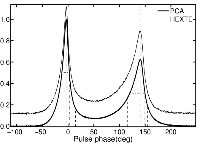
Figure 1: The total normalized profiles of the Crab pulsar measured by RXTE (PCA, MJD 51956–55927, 2–60 keV: thick line, HEXTE, MJD 51302–55927, 15–250 keV: thin line). The profiles were shifted with 0.0 and 0.12, respectively. Phase 0 represents the phase of the radio pulse. The two dotted lines represent the peak positions of the two pulses. The two dotted-dashed lines around P1 denote the phase range in which the flux was integrated, and the two dotted-dashed lines around P2 have the same meaning. The dashed lines are similar to the dotted-dashed lines but represent the phase ranges defined in Kuiper et al. (2001).

If the X-ray profile of the Crab pulsar showed detectable secular changes, the ratio curve between the normalized profiles in different epochs should deviate from a uniform distribution. The total profiles obtained from the 11-year observations of PCU0234 and HEXTE are shown in Figure 1, in which the PCA profile shows a much higher statistics than the HEXTE one. Therefore, two groups of profiles obtained from PCA data that obtained in time range of MJD 51955(2001-02-15)–52500(2002-08-14) and MJD 55254(2010-02-27)–55927(2012-01-01), were created, and then merged into two integrated profiles named Profile1 and Profile2, respectively. These two integrated profiles are used to produce the ratio curve. In order to eliminate the effect of the different background levels in these two periods, the two integrated profiles were reformed as follows: (1) subtract the background level that is determined by the mean flux per bin in phase 226.8 to $298.8\,\textordmasculine$ as Ge et al. (2012); (2) normalize the pulse profile to make the integrated flux, which is the sum of the flux per bin times the phase bin size, equal to 1; (3) add 9.0 to the value in each bin, because the total background count rate is about 9 times as high as the count rate of the pulses; and (4) normalize the pulse profile again. After these steps, the Profile2 to Profile1 ratio was obtained as shown in Figure 2b.

As can be seen clearly in Figure 2b, the distribution of the ratio is not uniform, with the $\chi^{2}$ of 63.2 for 17 points. The ratio at P1 (phase: -7.2 to $7.2\,\textordmasculine)$ is higher than 1.0 with the mean of 1.0016, and lower than 1.0 with mean of 0.9994 at the bridge(50.4–$90\,\textordmasculine$, as defined in Kuiper et al. (2001)). Compared to P1, P2 shows different behaviors that the ratio is around 1.0 at the leading edge (phase: 126–$144\,\textordmasculine$) and is higher than 1.0 at the trailing edge (phase: 144–$158\,\textordmasculine$). The deviation of the profile ratio curve from a uniform distribution implies that the X-ray profile evolved with time: after a few years, P1 became sharper and the distance between P1 and P2 increased a little bit.

3.2 Parameterization of the X-ray profile

Since the X-ray profile of the Crab pulsar has a typical double-peak structure, we used four parameters, including separation ($\Phi$), flux ratio ($R_{f}$), and widths ($W_{1}$ $\&$ $W_{2}$) of P1 and P2, to quantify the X-ray profile. $\Phi$ is the relative phase distance between the two maxima of the pulses. $W_{1}$ and $W_{2}$ are defined as the full width at half maximum (FWHM) of P1 and P2 after subtracting the pulse background (phase 226.8–$298.8\,\textordmasculine$). $R_{f}$ is the ratio between the integrated fluxes of P1 (-12.24 to $2.52\,\textordmasculine$) and P2 (123.84–$153.36\,\textordmasculine$), i.e., the integrated flux within the FWHM of the two pulses.

The fluxes of P1 and P2 (as well as their errors) could be obtained directly, but more calculations are needed for $\Phi$, $W_{1}$ and $W_{2}$ to have accuracy finer than the bin size. To obtain the accurate peak position and width of a pulse, we fitted it using the empirical formula proposed by Nelson et al. (1970),

$$L(\phi-\phi_{0})=N\frac{1+a(\phi-\phi_{0})+b(\phi-\phi_{0})^{2}}{1+c(\phi-\phi_{0})+d(\phi-\phi_{0})^{2}}e^{-f*(\phi-\phi_{0})^{2}}+l$$ (1)

where $L$ is the intensity at phase $\phi$, $l$ the baseline of the pulse profile, $\phi_{0}$ the phase shift, $N$ the pulse height of the profile, and $a$, $b$, $c$, $d$ and $f$ the shape coefficients. The pulse phase is measured in degrees. In the fitting, P1 was chosen in the phase range -27 to $12.78\,\textordmasculine$ and P2 in 109.8 to $167.4\,\textordmasculine$.

The peak separation $\Phi$ is calculated with the following steps(similar with Ge et al. (2012)): (1) Fit the two pulses of the total profile with Nelson’s formula and obtain their shape coefficients $a$, $b$, $c$, $d$, $f$, as well as $N$, $l$, and $\phi_{0}$, which are listed in Table. 2; (2) For an integrated profile in a time period and from which we want to get $\Phi$, fit its two pulses using the Nelson formula with $N$, $\phi_{0}$, and $l$ free and the other shape coefficients fixed to the values in Table. 2; (3) From the positions of the two maxima of the fitted profiles get their separation.

$W_{1}$ and $W_{2}$ were obtained in a similar way. We fitted the observed profile with the Nelson’s formula with all the coefficients free, and then the FWHMs of the fitted profiles were taken as the widths of P1 and P2.

We estimated the errors of $\Phi$, $W_{1}$ and $W_{2}$ with a Monte Carlo method. 100 simulated profiles were created by sampling from the original profile under the assumption that the photon counts in every phase bin follow the Poisson distribution. Then these simulated profiles were fitted with Nelson’s formula and 100 groups of $\Phi$, $W_{1}$, and $W_{2}$ values were obtained. The distribution widths of these values can represent their statistical errors, and the 1$\sigma$ width of the Gaussian function fit to the distribution of a parameter was taken as its 1$\sigma$ error.

3.3 Profile evolution with time

To study the evolution of $\Phi$, $R_{f}$, $W_{1}$ and $W_{2}$, we divide the PCA observations into 6 groups with roughly equal time span of about 660 days. In one group an integrated profile was produced and a set of $\Phi$, $R_{f}$, $W_{1}$ and $W_{2}$ were derived, so we have 6 data points for every parameter from the PCA observations. Because the source photons collected by HEXTE are much less than that by PCA, two profiles and thus two set of data points from HEXTE data were obtained in time ranges MJD 51302(1999-03-08)–54789(2008-11-19) and MJD 52570(2002-10-23)–55927(2012-01-01), respectively.

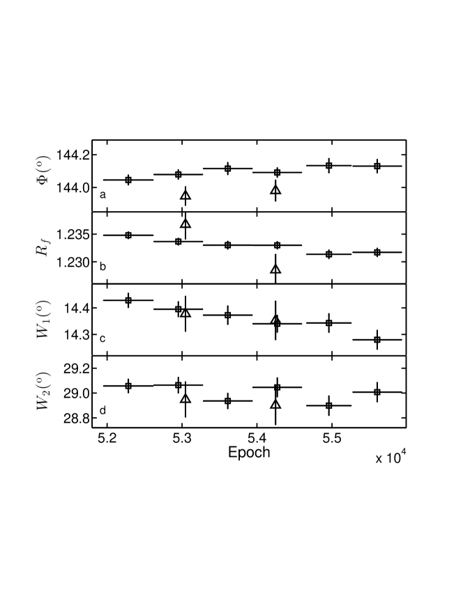
Figure 3: The profile parameters of the Crab pulsar from PCA (squares) and HEXTE (triangles) observations. Panels $a$, $b$, $c$ and $d$ show the peak separation ($\Phi$), flux ratio ($R_{f}$), and widths ($W_{1}$ $\&$ $W_{2}$) of P1 and P2, respectively. The data points of ${R}_{f}$, ${W_{1}}$ and ${W_{2}}$ from HEXTE data were shifted by $-0.273$, $-0.5\,\textordmasculine$ and $-0.7\,\textordmasculine$, respectively.

Figure 3 displays $\Phi$, $R_{f}$, $W_{1}$, and $W_{2}$ of the Crab pulsar measured from PCA and HEXTE. The parameters of the PCA profiles show large differences from the HEXTE ones, because the X-ray profile varies with energy (Mineo et al., 1997; Massaro et al., 2006). However, the variation trends of the parameters from these two instruments are similar. The peak separation $\Phi$ increased with time and the other parameters decreased with time.

3.3.1 Profile evolution results from the PCA data

The PCA data were first chosen to study the profile evolution using the four parameters defined above, which were fitted with linear functions to derive their changing rates. As listed in Table 3, the evolutions of $R_{f}$ and $W_{1}$ were detected with a high significance: the changing rate of $R_{f}$ is $-(3.52\pm 0.64)\times 10^{-2}$ per century, and that of $W_{1}$ is $1.45\pm 0.19\,\textordmasculine$ per century. The evolutions of $\Phi$ and $W_{2}$ are less significant, with $0.89\pm 0.26\,\textordmasculine$  and $-1.09\pm 0.95\,\textordmasculine$ per century, respectively. The changing rate of the peak separation is consistent with the result from (Ge et al., 2012) within 1$\sigma$ error, and the new result has a little bit higher significance. These quantitative results for the peak separation and flux ratio are consistent with the qualitative results deduced from the profile ratio curve.

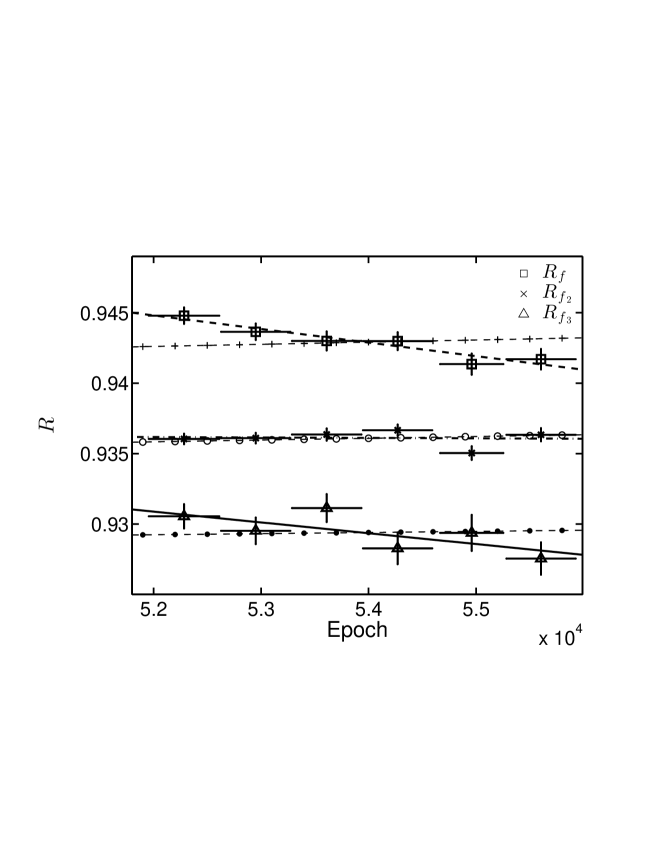
Figure 4: The pulse flux ratios of the Crab pulsar calculated in different phase ranges for PCA. The square points represent the ratios of the fluxes integrated in the FWHM of the two pulses ($R_{f}$) with $-0.29$ shifted, the cross points represent the ratios of the fluxes integrated in $-21.6$ to 14.4 º(for P1) and 115.2 to 154.8 º(for P2) ($R_{f_{2}}$), and the triangle points represent the ratios of the fluxes at the two peaks ($R_{f_{3}}$, shifted by 0.31). The dashed, dotted-dashed and solid lines are the fitted results for $R_{f}$, $R_{f_{2}}$ and $R_{f_{3}}$, respectively. Similarly, the thin dashed lines with “+”, empty and filled circles are the fitted results for $R_{f}$, $R_{f_{2}}$ and $R_{f_{3}}$ obtained from the faked profiles as described in Section 4.1. The phase ranges for the flux ratio calculation are shown in Figure 1.

The flux ratio of the two pulses should be different if the fluxes were integrated in different phase ranges. In order to get more information of the profile evolution, two more flux ratios were calculated with different phase ranges as shown in Figure 1. $R_{f_{2}}$ represents the integrated flux ratio of P1 (-21.6 to $14.4\,\textordmasculine$) and P2 (115.2–$154.8\,\textordmasculine$) (as defined in Kuiper et al. (2001)). The mean value of $R_{f_{2}}$ is 0.936(5), which is consistent with the result of Kuiper et al. (2001). $R_{f_{3}}$ is the peak flux ratio of P1 and P2, which has a mean value 0.619(1). As shown in Figure 4, the changing rates of $R_{f_{2}}$ and $R_{f_{3}}$ are $(-0.1\pm 0.8)\times 10^{-2}$ per century and $(-2.8\pm 1.5)\times 10^{-2}$ per century, respectively. Apparently, no evolution has been detected for $R_{f_{2}}$, while the changing rate of $R_{f_{3}}$ is close to $R_{f}$ but with a much lower significance. In any case, the changing rates of these two flux ratios are also significantly smaller than the radio results.

3.3.2 Joint study of the profile evolution with PCA and HEXTE

Figure 3 shows that the parameters infered from the HEXTE data show evolution similar to the PCA results, even though the parameters from two kinds of instruments have different mean values. With the assumption that the secular changes of the profile measured from PCA and HEXTE follow the same trends, the PCA and HEXTE parameters were shifted to around zero so that the $\chi^{2}$ of the linear fitting, which is defined by equation 2, reaches the minimum.

$$\chi^{2}=\frac{1}{N-3}\sum_{ij}(\frac{k(t_{ij}-t_{0})+b_{i}-\Phi_{ij}}{\sigma_{ij}})^{2}$$ (2)

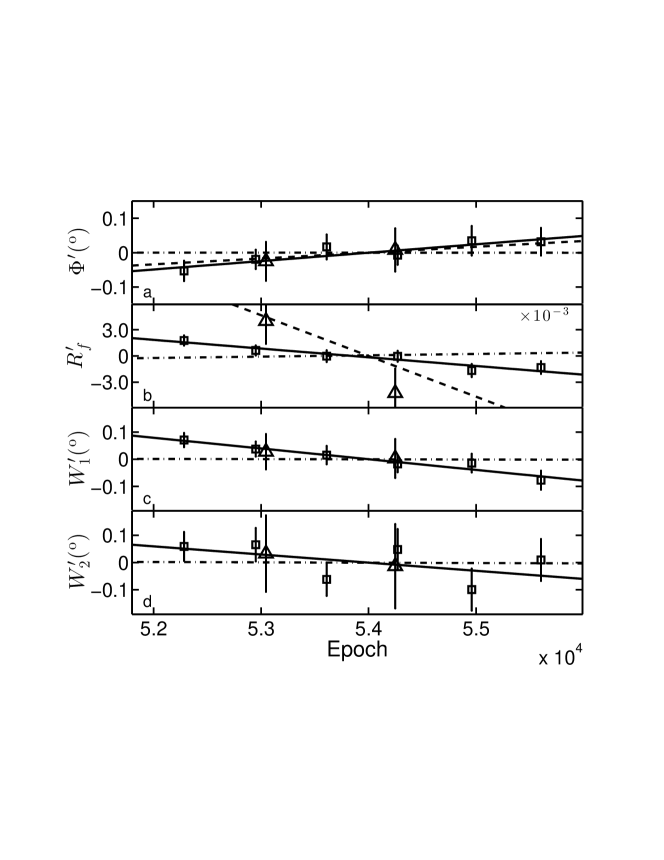
Figure 5: The corrected profile parameters from PCA (squares) and HEXTE (triangles). Panels $a$, $b$, $c$ and $d$ show the corrected parameters $\Phi^{\prime}$, $R_{f}^{\prime}$, $W_{1}^{\prime}$ and $W_{2}^{\prime}$, respectively. The dashed lines in panels $a$ and $b$ represent the radio results (Lyne et al., 2013), and the dotted-dashed lines are the fitted results of the parameters from the faked profile as shown in Figure 6.

where $N$ is the number of points, $k$ is the changing rate, $i$ is 0 or 1 to represent the data from PCA or HEXTE, $j$ denotes the data points from each instrument, $\Phi_{ij}$ is the peak separation, and $\sigma_{ij}$ the error of the peak separation obtained with the Monte-Carlo method described in section 3.1. The intercept $b_{i}$ correspond to the values at $t_{0}=54000$ in MJD format. The best estimation for $b_{i}$ was obtained when $\chi^{2}$ reached the minimum. Then, the corrected peak separation $\Phi^{\prime}$ was obtained with $b_{0}=144.10\,\textordmasculine$ and $b_{1}=143.98\,\textordmasculine$ subtracted. As presented in Figure 5, $\Phi^{\prime}$ increased linearly with time. $R_{f}$, $W_{1}$ and $W_{2}$ were processed with the same method, and the shifted intercepts for all these parameters are listed in Table 4.

$\Phi$, $R_{f}$, and $W_{1}$ inferred from the joint PCA and HEXTE data show secular changes similar to that from PCA data alone (Figure 5). The evolution of $W_{2}$ has not been significantly detected either, even with the HEXTE data added. The changing rate of the peak separation is $0.88\pm 0.20\,\textordmasculine$ per century, which is similar to the radio result, $0.62\pm 0.03\,\textordmasculine$ per century (Lyne et al., 2013). Ratio of the integrated fluxes within the FWHM of the two pulses descended with a rate $(3.64\pm 0.86)\times 10^{-2}$ per century, about 1/5 of the radio result, $(17.2\pm 0.8)\times 10^{-2}$ per century (Lyne et al., 2013). $W_{1}$ and $W_{2}$ descend with slopes of $1.44\pm 0.15\,\textordmasculine$ per century and $1.09\pm 0.73\,\textordmasculine$ per century, respectively.

4 Discussion

In this section, we will first study whether the observed profile evolution is due to the aging of the instruments, and then discuss the possible constraints of our results on the geometry of pulsar’s magnetosphere.

4.1 Profile changes induced by the aging of PCA

Previous studies have shown that the X-ray profile of the Crab pulsar varies with photon energy (Eikenberry and Fazio, 1997; Rots et al., 1998; Massaro et al., 2000; Willingale et al., 2001; Molkov et al., 2010; Ge et al., 2012), which can be also described quantitatively by the phase-resolved spectrum, and this has been studied in details by (Ge et al., 2012) using the PCA observations (from 2001-02-15 to 2009-11-07). Because the X-ray profiles we studied in this paper were integrated over the entire energy bands of the instruments, if the effective area of the instrument at different energies had gradual changes in the about 11 years of operation (Garcia et al., 2014), it could also result in pseudo changes of the X-ray profiles. In order to study the influence of the instrument aging on the observed profile evolution, we use the phase-resolved spectrum $F(\phi,E)$ measured from PCA (Ge et al., 2012) as input, convolve it with the effective area curves of PCU0234 in different epochs to fake the profiles, and from these profiles further derive the shape parameters in those epochs. Comparison of the shape parameters of the faked profiles and those of the observed ones will verify whether the profile evolution we found is intrinsic or not. The detailed process and results are given below.

The input profile $F(\phi,E)$ can be expressed as

$$F(\phi,E)=\beta(\phi)(E/E_{0})^{-\alpha(\phi)}\exp[{-N_{H}\sigma(E)}]$$ (3)

where the normalized flux $\beta(\phi)$ and photon index $\alpha(\phi)$ were inferred from Ge et al. (2012), $E$ is the photon energy in units of keV and $E_{0}=1$ keV, the absorption column density $N_{H}$ is $0.36\times 10^{22}$ cm^-2 (Ge et al., 2012), $\sigma(E)$ is the photo-electric cross-section (Morrison and McCammon, 1983). The number of input data from Table 5 of Ge et al. (2012) are not fine enough to get a smooth pulsed profile, so the normalized fluxes were fitted with two combined Nelson formula (Nelsonetal.(1970)andfourGaussianfunctions; whichweremainlyusedtofitfluxinthebridgeregion; andthefluxineachphasebinwasobtainedfromtheinterpolationofthefittedfunctions). The photon indices of the pulsed emission in (Ge et al., 2012) were first smoothed with a Gauss function that has an 1-sigma width of 3.6 degrees, and the smoothed photon indices were further fitted with an 18 order polynomial to get the photon index for a phase bin in this paper. Since there were only observed photon indices in the phase range greater than -48.6 and smaller than 196.2 (Ge et al., 2012) the polynomial function can not be constrained outside of this phase range. Therefore, the photon indices (of the pulsed emission) for bins with phases smaller than -48.6 degrees were fixed as 1.72, the value at -48.6 degrees, and for bins with phases greater than 192.2 degrees the photon indices were fixed as 2.17. The pulse profile $F_{P}(\phi)$, which is the phase resolved spectra (of the pulsar plus nebula) convolved with the response matrix, was obtained as follows

$$F_{P}(\phi)={\sum_{Ei}{F(\phi,E)RSP(E,i)}}\Delta{E}$$ (4)

where $RSP(E,i)$ is the average response matrix of PCU0234, and $\Delta{E}$ the input energy width at energy $E$.

The dead time of the instrument could also change the pulse profile, because the photon fluxes at different phases are not the same. We therefore calculated the dead time correction $DCOR$ using the formula:

$$DCOR=\frac{T}{T-DTF}$$ (5)

$$DTF=C\times{T}\times{dt}$$ (6)

where $T$ is the length for one phase bin, $C$ the photon counts from both the pulsar (Ge et al., 2012) and nebula (Garcia et al., 2014) in $T$, $dt$ the time for RXTE/PCA to process the information of one event (Jahoda et al., 2006), which is also called the dead time. $T$ was 33.6 $\mu$s because the profile was divided into 1000 phase bins in the calculation. The background events were also considered when we calculated $DTF$. The response profile has been divided by $DCOR$ when we produce the “final” faked profiles.

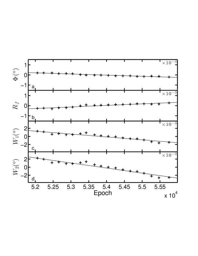
Figure 6: The parameters derived from the faked PCA profiles representing the influence of the aging of PCA. The solid lines are the linear fits to these parameters. The mean values of these parameters were subtracted as we were only interested in their variations.

Similar to what we did previously, using the faked profiles, we can obtain the ratio curve and parameter changes that induced by the instrument aging. The dashed line in the lower panel of Figure 2b represents the ratio of the faked profiles in MJD 51956–52500 (Profile3) and MJD 55254–55927 (Profile4). It is very different from the observed one and with a much smaller amplitude. The variations of $\Phi$, $R_{f}$, $W_{1}$, and $W_{2}$ induced by the aging of PCA are presented in Figure 6, and the linear fitting results are listed in Table 3. The changing rates are about 1 to 2 orders of magnitudes lower than the observed ones, and particularly for $\Phi$ and $R_{f}$, the instrument aging had secular changes opposite to the observed ones. Similarly, the changing rates $R_{f2}$ and $R_{f3}$ are $(0.29\pm 0.01)\times 10^{-2}$ per century and $(0.45\pm 0.01)\times 10^{-2}$ per century, which also had the secular changes opposite to the observed ones. Therefore, the contribution of the instrument aging to the observed pulse profile evolution is negligible.

4.2 Constrains on the geometry of the magnetosphere

The X-ray profile of the Crab pulsar shows secular changes that the peak separation of the profiles increases while the flux ratio and widths of the two pulses decrease with time. The evolutionary trends of the X-ray profile are similar to the radio results, which means that the magnetosphere evolution has a similar effect on emission regions of the X-ray and radio pulses.

For a simple magnetic dipole, the evolution of the magnetosphere axis is expected towards alignment rather than orthogonality (Lyne et al., 2013; Philippov et al., 2014; Arzamasskiy et al., 2015). However, the secular increases of the peak separations in the radio and X-ray bands are inconsistent with this expectation. Lyne et al. (2013) explained the evolution with geometrical model that inclination of the magnetic axis increases with time as the torque developed by the return current in the neutron star surface (Beskin et al., 2007). Based on the magnetohydrodynamic simulations (Philippov et al., 2014) and Arzamasskiy et al. (2015) pointed out that it is the magnetic dipole precession behavior with a characteristic time of 100 yr. The similar evolutionary rates of the X-ray and radio peak separations imply that the two kinds of emission locates at similar latitudes.

The evolution in the relative flux densities of the radio components are explained as highly coherent. Narrow beam and small structural magnetosphere changes might cause large effects on the component flux densities (Lyne et al., 2013). However, the changing rate of $R_{f}$, $(3.64\pm 0.86)\times 10^{-2}$ per century, is significantly lower than the radio result, $(17.2\pm 0.8)\times 10^{-2}$ per century. The difference even became bigger if wider phase intervals were chosen in calculating the integrated fluxes. This means that the X-ray emitting region is much larger than the radio emitting region, consistent with those represented by the widths of the radio and X-ray pulses. Therefore, a more complicated model is needed to explain the overall evolutionary behaviors of the radio and X-ray profiles, combined with the effects of the propagation time and the relativity (Morini, 1983).

5 Summary

In this paper, we found that the X-ray profile of the Crab pulsar had secular changes with time. The ratio curve of the two profiles in different epochs showed that, after a few years, P1 became sharper and the distance between P1 and the P2 increased a little bit. Quantitatively, the peak separation of the two pulses increased with $0.88\pm 0.20\,\textordmasculine$ per century, ratio of the integrated flux of P1 to that of P2 decreased with $(3.64\pm 0.86)\times 10^{-2}$ per century, and the widths of the P1 and P2 changed with $-1.44\pm 0.15\,\textordmasculine$ per century and $-1.09\pm 0.73\,\textordmasculine$ per century, respectively. These evolutionary trends are similar to the radio trends, although the values are different. A more complicated model of pulsar emission geometry is needed to explain the radio and X-ray results simultaneously.

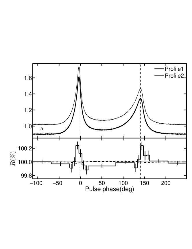
Figure 2: The two X-ray profiles of the Crab pulsar obtained by PCA in different time periods and their ratio curves. Panel $a$ shows Profile1 (thick line, integrated in MJD 51956 to 52500) and Profile2 (thin line, in MJD 55254 to 55927, shifted by a value of 0.12). The solid line in panel $b$ shows the Profile2 to Profile1 ratio, and the dashed line represents the faked ratio curve induced by the instrument aging as described in section 4.1. The two vertical lines denote the peak positions of the two pulses.

Table 1: The observation list of RXTE used in this work

Obs ID	Start Date	End Date	offset(’)	PCA exposure [s]	HEXTE exposure [s]
40093	1999-03-08	1999-03-22	0.03	–	13724
50098	2000-07-17	2000-07-21	0.03	–	5474
50099	2001-02-15	2001-08-27	0.03	7504	15466
60079	2001-09-10	2002-10-22	0.03	20240	18632
60080	2001-07-18	2001-07-20	0.03	3776	3701
60420	2001-09-07	2001-09-09	0.03	1824	1718
70018	2002-05-09	2003-05-14	0.03	9616	7024
70802	2002-11-07	2003-02-26	0.03	7888	7263
80802	2003-03-13	2004-02-15	0.03	17552	17221
90129	2004-11-15	2004-11-18	0.03	–	5946
90802	2004-02-29	2005-02-25	0.03	18032	16086
91802	2005-03-13	2006-02-10	0.03	17088	13971
92018	2006-05-10	2006-12-21	0.03	–	9774
92802	2006-03-11	2006-09-24	0.03	23536	25704
93802	2007-07-17	2008-12-17	0.03	28768	30164
94802	2008-12-31	2009-11-07	0.03	16768	13922
95802	2010-01-03	2010-12-08	0.03	29028	16229[1]
96382	2011-10-17	2011-12-11	0.03	8211	–
96802	2011-12-17	2012-01-01	0.03	19920	15301[1]
total exposure(s)				229751	231649

[1] Only cluster A data of HEXTE were used in our analyses.

Table 2: The coefficients of the Nelson’s formula for the main peak (P1) and the second peak (P2) of the Crab pulsar

		a	b	c	d	f	$\chi^{2}_{dof}$	d.o.f.
PCA	P1	-30.79	1550.04	-55.03	4521.40	568.32	2.0	92
	P2	-29.84	372.30	-42.00	1265.97	138.09	2.4	128
HEXTE	P1	-34.26	2351.16	-49.04	5971.22	667.86	2.0	92
	P2	-26.94	209.19	-45.95	887.59	131.46	1.7	128

Table 3: The changing rates of the X-ray profile parameters of the Crab pulsar

Instrument	$\Phi$	$R_{f}$	$W_{1}$	$W_{2}$
	( º/century)	($10^{-2}$)	( º/century)	( º/century)
PCA	$0.89\pm 0.26$	$-3.52\pm 0.64$	$-1.45\pm 0.19$	$-1.09\pm 0.95$
All[1]	$0.88\pm 0.20$	$-3.64\pm 0.86$	$-1.44\pm 0.15$	$-1.09\pm 0.73$
Resp[2]	$-0.004\pm 0.001$	$0.56\pm 0.01$	$-0.026\pm 0.001$	$-0.046\pm 0.001$
Radio[3]	$0.62\pm 0.03$	$-17.2\pm 0.8$	–	–

[1] The changing rates of the parameters from the joint PCA and HEXTE data. [2] The changing rates of the parameters from the faked profiles that represent the aging effect of PCA. [3] The radio results by (Lyne et al., 2013).

Table 4: The intercepts of the linear fitting to the profile parameters

Instrument	$\Phi$	$R_{f}$	$W_{1}$	$W_{2}$
	( º)		( º)	( º)
PCA	$144.10\pm 0.06$	$1.2330\pm 0.0012$	$14.36\pm 0.05$	$29.00\pm 0.12$
HEXTE	$143.98\pm 0.08$	$1.5058\pm 0.0038$	$14.85\pm 0.10$	$29.62\pm 0.20$

References

- Arzamasskiy et al. (2015) Arzamasskiy, L., Philippov, A., Tchekhovskoy, A. 2015, MNRAS, 453, 3540
- Beskin et al. (2007) Beskin, V. S., Nokhrina, E. E., 2007, Ap&SS, 308, 569.
- Cheng, Ho and Ruderman (1986a) Cheng, K. S., Ho, C., and Ruderman, M. 1986a, ApJ, 300, 500
- Cheng, Ho and Ruderman (1986b) Cheng, K. S., Ho, C., and Ruderman, M. 1986b, ApJ, 300, 522
- Chetana et al. (2011) Chetana, J., Biswajit, P. 2011, RAA, 11, 1134
- Daugherty and Harding (1996) Daugherty, J. K., and Harding, A. K. 1996, ApJ, 120, 107
- Eikenberry and Fazio (1997) Eikenberry, S. S., and Fazio, G. G. 1997, ApJ, 476, 281
- Garcia et al. (2014) Garcia, J. A., McClintock, J. E., Steiner, J. F., Remillard, R. A., and Grinberg, V. 2014, ApJ, 794, 73
- Ge et al. (2012) Ge, M. Y., Lu, F. J., Qu, J. L., Zheng, S. J., Chen, Y. and Han, D. W. 2012, ApJS, 199, 32
- Gold (1968) Gold, T. 1968, Nature, 218, 731
- Jahoda et al. (2006) Jahoda, K., Markwardt, C. B., Radeva, Y., Rots, A. H., et al. 2006, ApJ, 163, 401
- Kuiper et al. (2001) Kuiper, L., Hermsen, W., Cusumano, G., et al. 2001, A&A, 378, 918
- Lyne et al. (1993) Lyne, A. G., Pritchard, R. S. and Graham-Smith, F. 1993. MNRAS, 265, 1003
- Lyne et al. (2013) Lyne, A. G., Graham-Smith F., Weltevrede P., et al. 2013, Science, 342, 598
- Mineo et al. (1997) Mineo, T., Cusumano, G., Segreto, A., Massaro,E., et al. 1997, A&A, 327L, 21
- Massaro et al. (2000) Massaro, E., Cusumano, G., Litterio, M., and Mineo, T. 2000, A&A, 361, 695
- Massaro et al. (2006) Massaro, E., Campana, R., Cusumano, G., and Mineo, T. 2006, ApJ, 459, 859
- Molkov et al. (2010) Molkov, S., Jourdain, E., and Roques, J. P. 2010, ApJ, 708, 403
- Morini (1983) Morini, M., 1983, MNRAS, 202, 495
- Morrison and McCammon (1983) Morrison, R., McCammon, D. 1983, ApJ, 270, 119
- Nelson et al. (1970) Nelson, J., Hills, R., Cudaback, D., and Wampler, J. 1970, ApJ, 161, 235
- Philippov et al. (2014) Philippov, A. A., Spitkovsky, A. 2014, ApJ, 785, L33
- Patt et al. (1999) Patt, B. L., Ulmer, M. P., Zhang, W. et al. 1999, ApJ, 522, 440
- Rots et al. (1998) Rots, A. H., Jahoda, K., Macomb, D. J., Kawai, N., Saito, et al. 1998, ApJ, 501, 749
- Rots et al. (2004) Rots, A. H., Jahoda, K., and Lyne, A. G. 2004, ApJ, 605, L129
- Rothschild et al. (1998) Rothschild, R. E., Blanco, P. R. et al. 1998, A&A, 496, 538
- Standish (1990) Standish, E. M., Jr. 1990, A&A, 233, 252
- Sturner and Dermer (1994) Sturner, S. J., and Dermer, C. D. 1994, ApJ, 420, L79
- Willingale et al. (2001) Willingale, R., Aschenbach, et al. 2001, A&A, 365, 212
- Zanazzi and Lai (2015) Zanazzi, J. J. and Lai, D. 2015, MNRAS, 451, 695