An Implicit Form of Krasulina’s $k$-PCA
Update without the Orthonormality Constraint

Abstract

We shed new insights on the two commonly used updates for the online $k$-PCA problem, namely, Krasulina’s and Oja’s updates. We show that Krasulina’s update corresponds to a projected gradient descent step on the Stiefel manifold of the orthonormal $k$-frames, while Oja’s update amounts to a gradient descent step using the unprojected gradient. Following these observations, we derive a more implicit form of Krasulina’s $k$-PCA update, i.e. a version that uses the information of the future gradient as much as possible. Most interestingly, our implicit Krasulina update avoids the costly QR-decomposition step by bypassing the orthonormality constraint. We show that the new update in fact corresponds to an online EM step applied to a probabilistic $k$-PCA model. The probabilistic view of the updates allows us to combine multiple models in a distributed setting. We show experimentally that the implicit Krasulina update yields superior convergence while being significantly faster. We also give strong evidence that the new update can benefit from parallelism and is more stable w.r.t. tuning of the learning rate.

Introduction

Principal Component Analysis (PCA) (?) is one of the most widely used techniques in data analysis (?), dimensionality reduction (?), and machine learning (?). The problem amounts to finding projections of the $d$-dimensional data along $k<d$ orthogonal directions such that the expected variance of the reconstruction error is minimized. Formally, let $\mathrm{y}\in\mathbb{R}^{d}$ be a zero-mean random variable. In the vanilla $k$-PCA problem we seek a $d\times d$ projection matrix $\mathrm{P}$ of rank-$k$ such that the compression loss of $\mathrm{y}$,

$$\ell_{\text{comp}}(\mathrm{P}) =\mathbb{E}\big{[}\|\mathrm{P}\,\mathrm{y}-\mathrm{y}\|^{2}\big{]}=\text{tr}\big{(}(\mathrm{I}_{d}-\mathrm{P})\,\mathbb{E}[\mathrm{y}\,\mathrm{y}^{\top}]\big{)},\!\!\!\!$$ (1)

is minimized. Here $\mathrm{I}_{d}$ denotes the $d\times d$ identity matrix.

The optimum projection matrix can be decomposed as $\mathrm{P}^{*}=\mathrm{C}\,(\mathrm{C}^{\top}\mathrm{C})^{-1}\mathrm{C}^{\top}\coloneqq\mathrm{C}\,\mathrm{C}^{\dagger}$, where $\mathrm{C}$ is a $d\times k$ matrix that spans the space of top-$k$ eigenvectors of the data covariance matrix $\mathbb{E}\big{[}\mathrm{y}\,\mathrm{y}^{\top}\big{]}$. For a given $\mathrm{C}$, we denote by $\mathrm{x}\coloneqq\mathrm{C}^{\dagger}\,\mathrm{y}\in\mathbb{R}^{k}$, the projection of $\mathrm{y}$ onto the column space of $\mathrm{C}$. The reconstruction of $\mathrm{y}$ from the projection $\mathrm{x}$ can be calculated as $\mathrm{C}\,\mathrm{x}\in\mathbb{R}^{d}$. In practice, (1) is approximated using a finite number of samples $\{\mathrm{y}_{n}\}_{n=1}^{N}$ resulting in the following objective:

$$\hat{\ell}_{\text{comp}}(\mathrm{P}) =\nicefrac{{1}}{{N}}\,\text{tr}\big{(}(\mathrm{I}_{d}-\mathrm{P})\,\sum_{n}\mathrm{y}_{n}\,\mathrm{y}_{n}^{\top}\big{)}$$ (2)

$$=\nicefrac{{1}}{{N}}\,\text{tr}\big{(}(\mathrm{I}_{d}-\mathrm{P})\,\mathrm{Y}\,\mathrm{Y}^{\top}\big{)}\,.$$

Here, $\mathrm{Y}$ denotes the $d\times N$ matrix of observations, i.e. the $n$-th column is $\mathrm{y}_{n}$ We also define $\mathrm{X}$ as the matrices of the projected samples. Note that the objective (2) is linear and thus convex in $\mathrm{P}=\mathrm{C}\mathrm{C}^{\dagger}$, but non-convex in $\mathrm{C}$. Nevertheless, the solution can be efficiently calculated using the SVD of the empirical data covariance matrix $\mathrm{Y}\mathrm{Y}^{\top}$.

Although the original PCA problem concerns the full-batch setting, in many cases the dataset might be too large to be processed by a batch solver. In such scenarios, online PCA solvers that process a mini-batch (or a single observation) at a time are more desirable. In the online setting, two elegant solutions proposed by Krasulina (?) and Oja (?) for finding the top-$1$ direction have received considerable attention and been studied extensively throughout the years (?; ?; ?; ?). In the following, we review the generalizations of these two algorithms to the $k$-PCA problem.

We show that both the Krasulina and Oja updates correspond to stochastic gradient descent steps on the compression loss (and its reduced form) using the gradient of the loss at the old parameter. Using the terminology introduced in (?), we call updates that are based on the old gradient the explicit updates. In this paper, we focus on deriving a more implicit form of Krasulina’s updates. Implicit here means that the updates are based on the future gradients at the updated parameters. As an example, consider the following regularized loss minimization over the parameter $\uptheta$

$$\uptheta_{t+1}=\mathop{\mbox{argmin}}_{\uptheta}\big{(}\nicefrac{{1}}{{2\eta}}\,\|\uptheta-\uptheta_{t}\|^{2}+\text{loss}(\uptheta)\big{)}\,,$$ (3)

with learning rate $\eta>0$. Setting the derivative w.r.t. $\uptheta$ to zero yields the following gradient descent update

$$\uptheta_{t+1}=\uptheta_{t}-\eta\,\nabla\text{loss}(\uptheta_{t+1}).$$ (4)

The above update is referred to as an implicit gradient descent update since it uses the gradient of the loss at the future parameter $\uptheta_{t+1}$. In cases where solving the update using the gradient at the future estimate is infeasible, the update is usually approximated by the gradient at the current estimate

$$\uptheta_{t+1}\approx\,\uptheta_{t}-\eta\,\nabla\text{loss}(\uptheta_{t})\,,$$ (5)

which is referred to as the explicit gradient descent update. In many settings, implicit updates are more stable and have better convergence properties compared to their explicit counterparts (?; ?).

In summary:

• We first formulate the Krasulina and Oja updates as an online (un)projected gradient descent steps on the Stiefel manifold.

• Using this observation, we derive a more implicit form for Krasulina’s update for the $k$-PCA problem that avoids the orthonormality constraint and is strikingly simple.

• We show that the new implicit Krasulina update actually amounts to an online EM step on a probabilistic $k$-PCA model. This allows combining multiple $k$-PCA models in a distributed setting using the recent framework of (?).

• With an extensive set of experiments, we show that the implicit Krasulina update yields better convergence while being more stable w.r.t. the choice of initial learning rate. Furthermore, by avoiding the orthonormalization step and maintaining matrix pseudo-inverses instead, we achieve a much faster update. Further speedup can be achieved by running our algorithm in parallel and combining the results.

Related Work

Many efficient solvers have been developed for the vanilla PCA problem (2) throughout the years. For a reasonable data size, one can find the exact solution by applying a truncated SVD solver on the empirical data covariance matrix. Randomized SVD solvers (?) and power methods (?) are common alternatives when the size of the dataset is larger. Online PCA solvers are desirable when the data comes in as a stream or when a full pass over the data may not be feasible due to the large size of the dataset. In general, the online algorithms iteratively perform the updates using a mini-batch of observations (commonly a single observation) at every round. Among the online algorithms, Oja’s update (?) and its variants are the most well-studied (?; ?). Noticeably, Shamir (?) showed exponential convergence on a variance reduced variant of Oja’s algorithm. However, the algorithm requires multiple passes over the data. On the other hand, a thorough convergence analysis of Krasulina’s algorithm and its extension to the $k$-PCA problem is still lacking. A partial analysis was done recently in (?) where an exponential convergence was shown when the data covariance matrix has low rank. However, this assumption might be too restrictive in real-world scenarios. A lower expected rate of $\mathcal{O}(\nicefrac{{1}}{{t}})$ still holds for Krasulina’s $1$-PCA update for high rank data (?). Other formulations for online PCA exploit the linearity of the objective (1) in $\mathrm{P}$ by essentially maintaining a mixture of solutions for $\mathrm{P}$ of rank $k$ as a capped density matrix (?; ?). This approach leads to algorithms with optimal regret bounds (?) but these algorithms are fundamentally less efficient than the incremental counterparts that aim to optimize $\mathrm{C}$. However, inspired by this approach of optimizing for $\mathrm{P}$, an incremental heuristic method has been developed (?) that gives reasonable experimental convergence, but again suffers from high computational cost for the updates.

Quadratic Program on the Stiefel Manifold

Given the zero-mean random variable $\mathrm{y}\in\mathbb{R}^{d}$, consider the following optimization problem for the centered $k$-PCA problem:

$$\mathrm{C}^{*} =\mathop{\mbox{argmin}}_{\mathrm{C}\in\text{St}_{(d,k)}}\ell_{\text{comp}}(\mathrm{C})\,,$$ (6)

$$\text{ for\,\,\, }\ell_{\text{comp}}(\mathrm{C}) \coloneqq\nicefrac{{1}}{{2}}\,\mathbb{E}\big{[}\|\mathrm{C}\mathrm{C}^{\top}\mathrm{y}-\mathrm{y}\|^{2}\big{]}\,,$$

where $\text{St}_{(d,k)}=\{\mathrm{C}\,\in\,\mathbb{R}^{d\times k}|\,\mathrm{C}^{\top}\mathrm{C}=\mathrm{I}_{k}\}$ with $d\geq k$ is the compact Stiefel manifold of orthonormal $d\times k$ matrices. We view $\text{St}_{(d,k)}$ as an embedded submanifold of $\mathbb{R}^{d\times k}$. The objective (6) is identical to the expected compression loss (1). Indeed when $\mathrm{C}\in\text{St}_{(d,k)}$, then $\mathrm{P}=\mathrm{C}\mathrm{C}^{\top}$ is a projection matrix. Also for $\mathrm{C}\in\text{St}_{(d,k)}$, we have $\mathrm{C}^{\top}\mathrm{C}=\mathrm{I}_{k}$. Thus, we can rewrite (6) as

$$\mathrm{C}^{*} =\mathop{\mbox{argmin}}_{\mathrm{C}\in\text{St}_{(d,k)}}\ell_{\text{var}}(\mathrm{C})\,,$$ (7)

$$\text{ for\,\,\, }\ell_{\text{var}}(\mathrm{C})\coloneqq\nicefrac{{1}}{{2}}\Big{(}\text{tr} \big{(}\mathbb{E}[\mathrm{y}\mathrm{y}^{\top}]\big{)}-\text{tr}(\mathrm{C}^{\top}\mathbb{E}[\mathrm{y}\mathrm{y}^{\top}]\,\mathrm{C})\Big{)}\,.$$

Thus minimizing the compression loss (6) is equivalent to maximizing the variance $\text{tr}(\mathrm{C}^{\top}\mathbb{E}[\mathrm{y}\mathrm{y}^{\top}]\,\mathrm{C})=\mathbb{E}[\|\mathrm{C}^{\top}\mathrm{y}\|^{2}]=\text{Var}[\mathrm{x}]$ of the projection $\mathrm{x}=\mathrm{C}^{\top}\mathrm{y}$. Note that although the values of the objectives (6) and (7) are identical when $\mathrm{C}\in\text{St}_{(d,k)}$, they might yield different updates for the gradient based methods as we shall see in the following.

A stochastic optimization procedure for solving (6) can be motivated similar to (3) where an inertia term is added to the loss to keep the updated parameters close to the current estimates, that is,

$$\mathrm{C}^{\text{new}}=\mathop{\mbox{argmin}}_{\widetilde{\mathrm{C}}\in\text{St}_{(d,k)}}\nicefrac{{1}}{{2}}\,\Big{(}\nicefrac{{1}}{{\eta}}\,\big{\|}\widetilde{\mathrm{C}}-\mathrm{C}\big{\|}^{2}_{\text{F}}+\mathbb{E}\big{[}\|\widetilde{\mathrm{C}}\,\mathrm{x}-\mathrm{y}\|^{2}\big{]}\Big{)}\,,$$

where $\mathrm{x}=\widetilde{\mathrm{C}}^{\top}\mathrm{y}$ is the projection onto the column space of $\widetilde{\mathrm{C}}$ and $\|\mathrm{A}\|^{2}_{\text{F}}=\text{tr}(\mathrm{A}^{\top}\mathrm{A})$ denotes the squared Frobenius norm. A procedure for solving the optimization problem is based on iteratively applying a gradient descent step using the projected gradient of the objective onto the tangent space of $\text{St}_{(d,k)}$ at $\mathrm{C}$ followed by a retraction step (?). The tangent space at $\mathrm{C}\in\text{St}_{(d,k)}$ is characterized by $T(\mathrm{C})=\{\mathrm{G}\in\mathbb{R}^{d\times k}\,|\,\mathrm{G}^{\top}\mathrm{C}+\mathrm{C}^{\top}\,\mathrm{G}=\mathbf{0}_{k\times k}\}$ and the projected gradient of $\ell_{\text{comp}}$, denoted by $\overline{\nabla}\,\ell_{\text{comp}}$, can be obtained by projecting the Euclidean gradient $\nabla\ell_{\text{comp}}$ onto $T(\mathrm{C})$:

$$\nabla\ell_{\text{comp}} =\mathbb{E}[(\mathrm{C}\mathrm{C}^{\top}\mathrm{y}-\mathrm{y})\mathrm{y}^{\top}\mathrm{C}]\,,$$

$$\overline{\nabla}\,\ell_{\text{comp}}(\mathrm{C}) =(\mathrm{I}_{d}-\mathrm{C}\,\mathrm{C}^{\top})\,\nabla\ell_{\text{comp}}(\mathrm{C})$$

$$=\mathrm{C}\,\mathrm{C}^{\top}\,\mathbb{E}[\mathrm{y}\mathrm{y}^{\top}]\,\mathrm{C}-\mathbb{E}[\mathrm{y}\mathrm{y}^{\top}]\,\mathrm{C}=\nabla\ell_{\text{comp}}\,.$$

Notice that $\overline{\nabla}\,\ell_{\text{comp}}(\mathrm{C})=\nabla\ell_{\text{comp}}\in T(\mathrm{C})$. In a stochastic approximation setting, the gradient at each iteration is approximated by a given batch of observations $\{\mathrm{y}_{n}\}_{n=1}^{N}$:

$$\overline{\nabla}\,\hat{\ell}_{\text{comp}}(\mathrm{C}) =\nicefrac{{1}}{{N}}\sum_{n}\big{(}\mathrm{C}\,\mathrm{C}^{\top}\,\mathrm{y}_{n}\mathrm{y}_{n}^{\top}\mathrm{C}-\mathrm{y}_{n}\mathrm{y}_{n}^{\top}\mathrm{C}\big{)}$$ (8)

$$=\nicefrac{{1}}{{N}}\,(\mathrm{C}\mathrm{X}-\mathrm{Y})\mathrm{X}^{\top}\,,$$

where $\mathrm{Y}\in\mathbb{R}^{d\times N}$ denotes the matrix of observations and $\mathrm{X}\coloneqq\mathrm{C}^{\top}\mathrm{Y}$. Thus, the stochastic approximation update becomes

$$\widetilde{\mathrm{C}}=\mathrm{C}-\eta\,\overline{\nabla}\,\hat{\ell}_{\text{comp}}(\mathrm{C}) =\mathrm{C}-\nicefrac{{\eta}}{{N}}\,(\mathrm{C}\,\mathrm{X}-\mathrm{Y})\,\mathrm{X}^{\top}$$ (9)

$$\text{ and }\,\,\,\mathrm{C}^{\text{new}} =\text{{QR}}(\widetilde{\mathrm{C}})\,.$$

The intermediate parameter $\widetilde{\mathrm{C}}\notin\text{St}_{(d,k)}$ in general, but the second QR step ensures that $\mathrm{C}^{\text{new}}\in\text{St}_{(d,k)}$. This update (9) is identical to the extension of Krasulina’s update to the $k$-PCA problem which was proposed recently in (?).

Alternatively, the Euclidean gradient of (7) becomes

$$\nabla\ell_{\text{var}}(\mathrm{C})=-\mathbb{E}\big{[}\mathrm{y}\,\mathrm{y}^{\top}\big{]}\mathrm{C}\,.$$

Projecting this gradient onto the tangent space yields

$$\overline{\nabla}\,\ell_{\text{var}}(\mathrm{C})=(\mathrm{I}_{d}-\mathrm{C}\,\mathrm{C}^{\top})\,\nabla\ell_{\text{var}}(\mathrm{C})=\nabla\ell_{\text{comp}}(\mathrm{C})\,.$$

Thus the update using the projected gradient $\overline{\nabla}\,\ell_{\text{var}}(\mathrm{C})$ again yields Krasulina’s update for $k$-PCA (9). Interestingly, the update using the Euclidean (unprojected) gradient $\nabla\hat{\ell}_{\text{var}}(\mathrm{C})$ gives the well-known Oja update for $k$-PCA (?):

$$\widetilde{\mathrm{C}}=\mathrm{C}-\eta\,\nabla\hat{\ell}_{\text{var}}(\mathrm{C}) =\mathrm{C}+\nicefrac{{\eta}}{{N}}\,\mathrm{Y}\,\mathrm{Y}^{\top}\,\mathrm{C}\,,$$

$$\text{ and }\,\,\,\mathrm{C}^{\text{new}} =\text{{QR}}(\widetilde{\mathrm{C}})\,,$$

Thus, Oja’s update is a an stochastic approximation update that aims to maximize the variance of the projection, but ignores the structure of the tangent space of the Stiefel manifold.

Note that both the Krasulina and Oja updates are explicit (similar to gradient descent update (5)) in that they use the gradient at the old parameter $\mathrm{C}$ rather than the new parameter $\mathrm{C}^{\text{new}}$ (?). Unfortunately, using the new parameter $\mathrm{C}^{\text{new}}$ for the updates as in (4) does not yield a tractable solution. However, we will show that a more implicit form of Krasulina’s update, i.e. the one that uses the gradient at the new parameter, can be achieved when the orthonormality constraint is abandoned.

New Update w.o. Orthonormality Constraint

Instead of maintaining an orthonormal matrix $\mathrm{C}$, we let $\mathrm{C}$ be any $d\times k$ matrix of rank-$k$ and use the fact that the projection of an observation $\mathrm{y}\in\mathbb{R}^{d}$ onto the column space of $\mathrm{C}$ corresponds to $\mathrm{C}^{\dagger}\,\mathrm{y}\in\mathbb{R}^{k}$:

$$\mathrm{C}^{\text{new}}=\mathop{\mbox{argmin}}_{\widetilde{\mathrm{C}}}\,\nicefrac{{1}}{{2}}\,\Big{(}\nicefrac{{1}}{{\eta}}\,\big{\|}\widetilde{\mathrm{C}}-\mathrm{C}\big{\|}^{2}_{\text{F}}\\ +\mathbb{E}\big{[}\|\widetilde{\mathrm{C}}\,\mathrm{x}-\mathrm{y}\|^{2}\big{]}\Big{)}\,,$$ (10)

where $\mathrm{x}=\mathrm{C}^{\dagger}\,\mathrm{y}$ is the projection using the old matrix $\mathrm{C}$. Setting the derivatives w.r.t. $\widetilde{\mathrm{C}}$ to zero, we obtain

$$\mathrm{C}^{\text{new}} =\mathrm{C}-\eta\mathbb{E}\big{[}(\mathrm{C}^{\text{new}}\mathrm{x}-\mathrm{y})\,\mathrm{x}^{\top}\big{]}$$

$$=\Big{(}\mathbb{E}[\,\mathrm{y}\mathrm{x}^{\top}]+\nicefrac{{1}}{{\eta}}\,\mathrm{C}\Big{)}\Big{(}\mathbb{E}[\,\mathrm{x}\mathrm{x}^{\top}]+\nicefrac{{1}}{{\eta}}\,\mathrm{I}_{k}\Big{)}^{-1}.$$

For a batch of points $\{\mathrm{y}_{n}\}_{n=1}^{N}$, this new update, which we call the implicit Krasulina update, becomes

$$\boxed{\mathrm{C}^{\text{new}}=\!\Big{(}\nicefrac{{1}}{{N}}\,\mathrm{Y}\mathrm{X}^{\top}\!\!+\nicefrac{{1}}{{\eta}}\,\mathrm{C}\Big{)}\Big{(}\nicefrac{{1}}{{N}}\,\mathrm{X}\mathrm{X}^{\top}\!\!+\nicefrac{{1}}{{\eta}}\,\mathrm{I}_{k}\Big{)}^{-1}}\,.$$ (11)

Note that an explicit variant can also be obtained by simply approximating $\mathrm{C}^{\text{new}}\,\mathrm{X}$ in the derivative equation by the old matrix $\mathrm{C}\,\mathrm{X}$:

$$\mathrm{C}^{\text{new}}\approx\,\,\mathrm{C}\,-\,\,\nicefrac{{\eta}}{{N}}\,\big{(}\mathrm{C}\,\mathrm{X}-\mathrm{Y}\big{)}\mathrm{X}^{\top}.$$

This is update (9) without enforcing the orthonormality constraint using the QR decomposition and in which the projection is calculated using $\mathrm{C}^{\dagger}$ instead of $\mathrm{C}^{\top}$.

A few additional remarks are in order. First, it may seem plausible to replace the projected gradient term $\overline{\nabla}\,\hat{\ell}_{\text{comp}}(\mathrm{C})$ in (9) with a more recent projected gradient $\overline{\nabla}\,\hat{\ell}_{\text{comp}}(\widetilde{\mathrm{C}})$ to achieve an implicit update similar to (11). However, note that $\widetilde{\mathrm{C}}\notin\text{St}_{(d,k)}$ in general and thus, this would not correspond to a valid projected gradient update. Avoiding the orthonormality constraint assures that the future gradient is indeed a valid descent direction. Additionally, note that (11) is only partially implicit since we use the old $\mathrm{C}$ for finding the projection $\mathrm{X}$. Unfortunately, the fully implicit update does not yield a closed form solution.

The implicit update (9) has a simple form in the stochastic setting, when a single observation $\mathrm{y}_{t}$ is received at round $t$. Let $\mathrm{x}_{t}=\mathrm{C}^{\dagger}\,\mathrm{y}_{t}$ denote the projection. Applying the Sherman-Morrison formula (?) for the inverse of rank-one matrix updates, we can write (11) as

$$\boxed{\mathrm{C}^{\text{new}}=\mathrm{C}-\frac{\eta}{1+\eta\,\|\mathrm{x}_{t}\|^{2}}\,\,(\mathrm{C}\,\mathrm{x}_{t}-\mathrm{y}_{t})\,\mathrm{x}_{t}^{\top}}\,.$$ (12)

which we call the stochastic implicit Krasulina update. Note that the learning rate $\frac{\eta}{1+\eta\|x_{t}\|^{2}}$ in (12) is essentially inversely proportional to the norm of the individual projection $\mathrm{x}_{t}$. The same fractional form of the learning rate appears in the implicit update for online stochastic gradient descent for linear regression (?; ?) which coincides with the differently motivated “normalized LMS” algorithm of (?). As noted in (?), implicit updates have slower initial convergence (due to the smaller learning rate) and smaller final error rate compared to the explicit updates. Also, as a result of the adaptivity of the learning rate, the implicit Krasulina update becomes less sensitive to the initial choice for the learning rate. We will show this in the experimental section.

input :   data stream $\mathrm{y}_{t}\,,t=1,\ldots,T$

output :   projection matrix $\mathrm{P}=\mathrm{C}\mathrm{C}^{\dagger}$

initialize  $\mathrm{C}$  and set  $\mathrm{C}^{\dagger}=(\mathrm{C}^{\top}\mathrm{C})^{-1}\mathrm{C}^{\top}$ for $t\leftarrow 1$ to $T$ do

       $\mathrm{x}_{t}\leftarrow\mathrm{C}^{\dagger}\mathrm{y}_{t}$

       $\mathrm{r}_{t}\leftarrow\mathrm{C}\,\mathrm{x}_{t}-\mathrm{y}_{t}$

       $\eta_{\mathrm{x}_{t}}\leftarrow\nicefrac{{\eta_{t}}}{{(1+\eta_{t}\,\|\mathrm{x}_{t}\|^{2})}}$

       $\mathrm{C}\leftarrow\mathrm{C}-\eta_{\mathrm{x}_{t}}\,\mathrm{r}_{t}\,\mathrm{x}_{t}^{\top}$

       $\mathrm{C}^{\dagger}\leftarrow\text{{RankOnePinvUpdate}}(\mathrm{C},\mathrm{C}^{\dagger},\eta_{\mathrm{x}_{t}}\mathrm{r}_{t},\mathrm{x}_{t})$

end for

$\mathrm{P}\leftarrow\mathrm{C}\mathrm{C}^{\dagger}$

return $\mathrm{P}$

Algorithm 1 Stochastic Implicit Krasulina Algorithm

Efficient Implementation

We provide some insight on the efficient implementation of the implicit Krasulina update. While our update avoids the costly QR step, it may impose extra computational complexity when calculating the projection. Namely, the computational complexity of the stochastic update (12) is dominated by the calculation of the matrix pseudo-inverse $\mathrm{C}^{\dagger}=(\mathrm{C}^{\top}\mathrm{C})^{-1}\mathrm{C}^{\top}$. In order to implement the stochastic updates efficiently, we can exploit the fact that each iteration involves a rank-$1$ update on matrix $\mathrm{C}$. One approach to reduce the computational complexity would be to maintain the inverse matrix $\mathrm{\Lambda}\coloneqq(\mathrm{C}^{\top}\mathrm{C})^{-1}$ and update it accordingly at every iteration. Note that a rank-$1$ update on $\mathrm{C}$ corresponds to a rank-$2$ update on $\mathrm{\Lambda}^{-1}$. Thus, the inverse can be carried out efficiently using the Woodbury matrix identity (?). The one-time complexity of calculating the inverse is $\mathcal{O}(k^{3})$, but can be significantly reduced by e.g. using a rectangular diagonal matrix as the initial solution. Thus, the overall complexity of the algorithm for the stochastic update (12) becomes $\mathcal{O}(k\,d)$.

A computationally more efficient approach is to directly keep track of the matrix $\mathrm{C}^{\dagger}$ and apply the rank-1 update for the Moore-Penrose inverse proposed in (?). The complexity of each rank-$1$ update amounts to $\mathcal{O}(k\,d)$. Our implicit Krasulina update is summarized in Algorithm 1, where the operator RankOnePinvUpdate is described in (?).

Probabilistic $k$-PCA and Online EM

We now provide an alternative motivation for our new implicit Krasulina update (11) as an instantiation of the recent online Expectation Maximization (EM) algorithm (?) for a certain probabilistic $k$-PCA model. This probabilistic $k$-PCA model was introduced in (?; ?) as a linear-Gaussian model:

$$\mathrm{y}=\mathrm{C}\,\mathrm{x} +\upnu\,,\,\,\,$$ (13)

$$\text{ where }\,\,\,\mathrm{x}\sim\mathcal{N}(\mathbf{0}_{k},\,\mathrm{I}_{k}) \text{ and }\,\,\,\upnu\sim\mathcal{N}(\mathbf{0}_{d},\,\mathrm{Q})\,.$$

where $\mathrm{x}$ is the $k\times 1$ unknown hidden state, $\upnu$ denotes the $d\times 1$ observation noise, and $\mathrm{C}\in\mathbb{R}^{d\times k}$. Also, $\mathcal{N}(\upmu,\mathrm{S})$ denotes a Gaussian distribution having mean $\upmu$ and covariance $\mathrm{S}$. Usually, the noise covariance is assumed to be isotropic, i.e. $\mathrm{Q}=\epsilon\,\mathrm{I}_{d}$. Note that since all random variables are Gaussian, the posterior distribution of the hidden state also becomes Gaussian, that is,

$$\mathrm{x}|\,\mathrm{y}\sim\mathcal{N}(\upbeta\,\mathrm{y},\,\mathrm{I}_{k}-\upbeta\,\mathrm{C})\,,\text{ where }\upbeta=\mathrm{C}^{\top}(\mathrm{C}\,\mathrm{C}^{\top}+\mathrm{Q})^{-1}.$$

An interesting case happens in the limit where the covariance of the noise $\upnu$ becomes infinitesimally small. Namely, in the limit $\mathrm{Q}=\lim_{\epsilon\rightarrow 0}\epsilon\,\mathrm{I}_{d}$, the likelihood of a point $\mathrm{y}$ is solely determined by the squared Euclidean distance between $\mathrm{y}$ and its reconstruction $\mathrm{C}\,\mathrm{x}$. The posterior of the hidden state collapses into a single point,

$$\mathrm{x}|\,\mathrm{y}\sim\mathcal{N}\big{(}(\mathrm{C}^{\top}\,\mathrm{C})^{-1}\mathrm{C}^{\top}\mathrm{y},\,\mathbf{0}\big{)}\,=\delta\big{(}\mathrm{x}-(\mathrm{C}^{\top}\,\mathrm{C})^{-1}\mathrm{C}^{\top}\mathrm{y}\big{)}\,,$$

where $\delta$ is the Dirac measure. Moreover, the maximum likelihood estimator for $\mathrm{C}$ is achieved when $\mathrm{C}$ spans the space of top-$k$ eigenvectors of the data covariance matrix (?). Thus, the linear-Gaussian model reduces to the vanilla $k$-PCA problem.

Using the probabilistic $k$-PCA formulation allows solving the vanilla $k$-PCA problem iteratively in the zero noise limit via the application of the EM algorithm (?). Let $\Theta=\{\epsilon,\mathrm{C}\}$ denote the set of parameters of the probabilistic latent variable model with joint probability density $P_{\Theta}(\mathrm{x},\mathrm{y})$. The EM upper-bound can be written as

$${\text{U}}_{\Theta^{(t)}}(\widetilde{\Theta}|\mathrm{Y}^{(t)})\!=-\nicefrac{{1}}{{N^{(t)}}}\sum_{n}\!\int_{\mathrm{x}}\!P_{\Theta^{(t)}}(\mathrm{x}|\,\mathrm{y}_{n})\log P_{\widetilde{\Theta}}(\mathrm{x},\mathrm{y}_{n})$$

$$=\frac{1}{2}\tilde{\epsilon}^{\scriptscriptstyle-1}\text{tr}\big{(}\widetilde{\mathrm{C}}\Sigma\widetilde{\mathrm{C}}^{\top}-\frac{2}{N}\mathrm{Y}\mathrm{X}^{\top}\widetilde{\mathrm{C}}^{\top}\big{)}+d\log\,\tilde{\epsilon}+\text{const.}$$ (14)

where $\mathrm{X}=\upbeta\,\mathrm{Y}$  with  $\upbeta=\mathrm{C}^{\top}(\mathrm{C}\,\mathrm{C}^{\top}+\epsilon\,\mathrm{I}_{k})^{-1}$ and $\Sigma=\mathrm{I}_{k}-\upbeta\mathrm{C}+\frac{1}{N}\,\mathrm{X}\mathrm{X}^{\top}$. We now consider the case when $\epsilon$ becomes infinitesimally small. Note that in the limit $\epsilon\rightarrow 0$, we have $\upbeta=(\mathrm{C}\,\mathrm{C}^{\top})^{-1}\,\mathrm{C}^{\top}=\mathrm{C}^{\dagger}$ and $\upbeta\,\mathrm{C}=\mathrm{I}_{k}$. Iteratively forming the EM upper-bound and minimizing it yields the following procedure (?):

$$\mathrm{X} =\mathrm{C}^{\dagger}\mathrm{Y}=(\mathrm{C}\,\mathrm{C}^{\top})^{-1}\,\mathrm{C}^{\top}\,\mathrm{Y}\,\,\,$$ (E-step)  , (15)

$$\mathrm{C}^{\text{new}} =\mathrm{Y}\mathrm{X}^{\dagger}=\mathrm{Y}\mathrm{X}^{\top}(\mathrm{X}\mathrm{X}^{\top})^{-1}\,\,\,$$ (M-step) ,

where the matrices $\mathrm{X}$ and $\mathrm{Y}$ are defined as before. Because of the tightness of the EM upper-bound, every step of the EM algorithm is guaranteed to either improve the compression loss or leave it unchanged (?). The final projection matrix is obtained as $\mathrm{P}=\mathrm{C}\mathrm{C}^{\dagger}$.

We now motivate our new implicit Krasulina update as online version of the update (15). This can be achieved by an application of a recent online EM algorithm developed in (?). In the online setting, the learner receives a mini-batch of observations (usually a single observation) at a time and performs parameter updates by minimizing the negative log-likelihood of the given examples. In order to make the learning stable, an inertia (aka regularizer) term is added to the loss to keep the updates close to the old parameters. Thus, the learner minimizes the combined inertia plus loss of the current iteration. Let $\mathrm{Y}^{(t)}\in\mathbb{R}^{d\times N^{(t)}}$ be the given batch of observations at round $t$. The online EM algorithm introduced in (?) is motivated in the same manner by minimizing the following loss at iteration $t$:

$$\Theta^{(t+1)}=\mathop{\mbox{argmin}}_{\widetilde{\Theta}}\,\Big{(}\nicefrac{{1}}{{\eta^{(t)}}}\,\Delta_{\text{RE}}(\Theta^{(t)},\widetilde{\Theta})+{\text{U}}_{\Theta^{(t)}}(\widetilde{\Theta}|\,\mathrm{Y}^{(t)})\Big{)}.$$

where $\Delta_{\text{RE}}(\Theta,\widetilde{\Theta})=\int_{\mathrm{x},\,\mathrm{y}}P_{\Theta}(\mathrm{x},\mathrm{y})\log\frac{P_{\Theta}(\mathrm{x},\mathrm{y})}{P_{\widetilde{\Theta}}(\mathrm{x},\mathrm{y})}$ is the relative entropy divergence between the joints and $\eta^{(t)}>0$ is the learning rate. In the following, we consider one iteration of the online EM algorithm and drop the $t$ superscript to avoid clutter.

We now consider the online EM algorithm when applied to the probabilistic $k$-PCA model (13). Note that $\Theta=\{\epsilon,\mathrm{C}\}$. We can write

$$\Delta_{\text{RE}}(\Theta,\widetilde{\Theta}) =\frac{d}{2}\big{(}\frac{\epsilon}{\tilde{\epsilon}}-\log\frac{\epsilon}{\tilde{\epsilon}}-1\big{)}$$ (16)

$$+\frac{1}{2}\,\tilde{\epsilon}^{\scriptscriptstyle-1}\,\text{tr}\big{(}(\mathrm{C}-\widetilde{\mathrm{C}})\,(\mathrm{C}-\widetilde{\mathrm{C}})^{\top}\big{)}\,,$$

We now consider the case where $\tilde{\epsilon}=\epsilon$ is fixed. Combining (16) and (14), the update for parameter $\mathrm{C}$ becomes

$$\mathrm{C}^{\text{new}}=\Big{(}\frac{1}{N}\mathrm{Y}\,\mathrm{X}^{\top}+\frac{\epsilon^{-1}}{\eta^{\prime}}\,\mathrm{C}\Big{)}\\ \times\,\Big{(}\mathrm{I}_{k}-\upbeta\,\mathrm{C}+\frac{1}{N}\,\mathrm{X}\,\mathrm{X}^{\top}+\frac{\epsilon^{-1}}{\eta^{\prime}}\,\mathrm{I}_{k}\Big{)}^{-1}\,\,\,\,\text{(M-step)}\,.$$

In order to recover the updates for the online $k$-PCA, we again need to consider the case when $\epsilon$ becomes infinitesimally small. Choosing $\eta^{\prime}(\epsilon)$ such that $\lim_{\epsilon\rightarrow 0}\nicefrac{{\epsilon^{-1}}}{{\eta^{\prime}}}=\nicefrac{{1}}{{\eta}}$  yields (11). Note that the E-step of the online EM algorithm becomes identical to (15). Also, the limit case $\eta\rightarrow 0$ keeps the parameters unchanged, i.e. $\mathrm{C}^{\text{new}}=\mathrm{C}$ and the case $\eta\rightarrow\infty$ recovers the batch EM updates (15).

Distributed Setting

The alternative view of the implicit Krasulina update (11) as an EM step allows combining multiple models in a distributed setting via the online EM framework introduced in (?). More specifically, given a set of $M$ hidden variable models parameterized by $\{\Theta^{(i)}\}_{i=1}^{M}$, the optimal combined model $\Theta^{*}$ corresponds to the minimizer of the following objective

$$\Theta^{*}=\mathop{\mbox{argmin}}_{\Theta}\,\sum_{i\in[M]}\alpha_{i}\,\Delta_{\text{RE}}(\Theta^{(i)},\Theta)\,,$$

where $\alpha_{i}\geq 0$ is the weight associated with model $i$. The weight of the model can be assigned based on the performance on a validation set or based on the number of observations processed by the model so far. For synchronous updates, we simply have $\alpha_{i}=\frac{1}{M}$. In a distributed online PCA setting, let $\mathrm{C}^{(i)}$ denote the matrix learned by the model $i$. By fixing $\epsilon$ for all the models and letting $\Theta^{(i)}=\{\epsilon,\mathrm{C}^{(i)}\}$, we have

$$\mathrm{C}^{*}=\frac{\sum_{i\in[M]}\alpha_{i}\,\mathrm{C}^{(i)}}{\sum_{i\in[M]}\alpha_{i}}\,.$$ (17)

The probabilistic view of our implicit Krasulina updates allows training multiple $k$-PCA models in parallel and combining them efficiently via simple averaging. Note that for the previous approaches, the $\mathrm{C}^{(i)},\,i\in[M]$ matrices are orthonormal and to the best of our knowledge, there is no systematic way of combining rank-$k$ orthonormal matrices. One trick would be to also average these matrices. However, the average of a set of orthonormal matrices does not necessarily yields an orthonormal matrix and a QR step is required after combining. As we will show experimentally, the heuristic of simply averaging the orthonormal matrices $\mathrm{C}^{(i)}$ produced by the Krasulina and Oja updates and then orthonormalizing the average yields poor empirical results. On the other hand, our new implicit Krasulina update produces arbitrary matrices $\mathrm{C}^{(i)}\in\mathrm{R}^{d\times k}$ and averaging those matrices (as advised by the online EM framework) results in excellent performance.

Experiments

In this section, we perform experiments on real-world datasets using our proposed implicit form of Krasulina’s update (12) and contrast the results with Oja’s, Krasulina’s, and the incremental algorithm (?). We perform experiments on MNIST dataset of $70000$ handwritten images with dimension $784$ and CIFAR-10 dataset of real-world images of dimension $3072$ having $60000$ images in total. We apply all the updates in a stochastic manner by sweeping over the data once. We consider a decaying learning rate of $\eta=\nicefrac{{\eta_{0}}}{{t^{\gamma}}}$  where $t$ denotes the iteration number, $0.5\leq\gamma<1$ is a constant, and $\eta_{0}$ denotes the initial learning rate. For each dataset, we randomly select 10% of the data as a validation set to select the optimal initial learning rate and the value of $\gamma$ for each algorithm. We use $\gamma=0.9$ for Krasulina’s and Oja’s methods and set $\gamma=0.8$ for our method. Note that the incremental algorithm does not require a learning rate. We report the performance on the full dataset. We repeat each experiment 10 times with a different random initialization and report the average. For comparison, we also calculate the result of the batch PCA solution using SVD decomposition of the empirical data covariance matrix for each experiment.

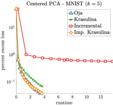
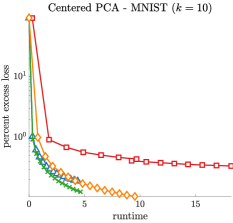
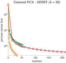
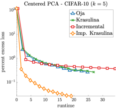
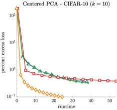
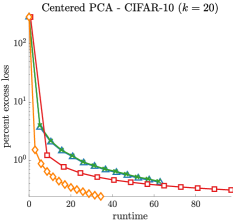
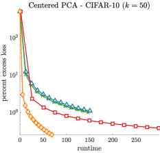
Figure 1: Centered online $k$-PCA: the results of different algorithms on the MNIST (top) and CIFAR-10 (bottom). The value of $k$ is shown on top of each figure. We plot the percentage of the excess loss which is defined as the normalized regret w.r.t to the best offline comparator (i.e. full-batch PCA). Each dot shows the progress of the algorithm in 1000 iteration intervals. Our proposed implicit Krasulina algorithm achieves the best convergence and provides the best runtime overall, especially when the values of $d$ and $k$ are large.

Method	$\eta_{0}$-Scale	MNIST			CIFAR10
		$k=5$	$k=10$	$k=20$	$k=5$	$k=10$	$k=20$
Batch PCA	–	$35.16$	$26.95$	$18.74$	$86.98$	$65.70$	$48.65$
Oja	$0.1\times$	$35.79\pm 0.38$	$29.78\pm 0.38$	$21.55\pm 0.25$	$116.26\pm 2.58$	$66.81\pm 0.58$	$58.28\pm 0.65$
	$1\times$	$35.19\pm 0.05$	$26.98\pm 0.02$	$18.80\pm 0.03$	$87.28\pm 0.43$	$65.90\pm 0.01$	$48.86\pm 0.05$
	$10\times$	$35.29\pm 0.01$	$27.08\pm 0.01$	$19.01\pm 0.01$	$87.22\pm 0.04$	$67.68\pm 0.13$	$50.36\pm 0.13$
Krasulina	$0.1\times$	$35.78\pm 0.37$	$29.92\pm 0.37$	$21.44\pm 0.24$	$116.86\pm 2.58$	$66.76\pm 0.65$	$57.62\pm 0.65$
	$1\times$	$35.17\pm 0.00$	$26.96\pm 0.01$	$18.79\pm 0.02$	$87.04\pm 0.52$	$65.90\pm 0.01$	$48.87\pm 0.05$
	$10\times$	$35.30\pm 0.01$	$27.09\pm 0.01$	$19.02\pm 0.02$	$87.17\pm 0.04$	$67.87\pm 0.16$	$50.56\pm 0.15$
Incremental	–	$35.26\pm 0.10$	$27.01\pm 0.04$	$18.83\pm 0.05$	$87.50\pm 0.46$	$65.75\pm 0.05$	$48.82\pm 0.10$
Imp. Krasulina	$0.1\times$	$35.17\pm 0.01$	$26.96\pm 0.01$	$18.78\pm 0.02$	$87.00\pm 0.00$	$65.75\pm 0.05$	$48.75\pm 0.03$
	$1\times$	$35.17\pm 0.01$	$26.97\pm 0.03$	$18.77\pm 0.02$	$87.01\pm 0.00$	$65.78\pm 0.09$	$48.74\pm 0.04$
	$10\times$	$35.17\pm 0.01$	$26.98\pm 0.05$	$18.77\pm 0.01$	$87.02\pm 0.04$	$65.74\pm 0.01$	$48.76\pm 0.03$

Table 1: Compression loss on different datasets using the optimal initial learning rate $\eta_{0}$ (selected using a validation set) and its scaling. Note that due to the adaptive form of learning rate, the results of our implicit Krasulina update is more stable w.r.t. to the choice of the initial learning rate.

Centered PCA

We show the results of the algorithms on the centered datasets in Figure 1 as a function of runtime. We plot the percentage of excess loss (i.e. normalized regret) w.r.t to the best achievable loss by an offline algorithm (i.e. full-batch PCA). Each dot shows the progress of the algorithm in 1000 iteration intervals. As can be seen, our implicit Krasulina update achieves the best convergence among all the algorithms. Additionally, our algorithm is considerably faster in most cases. Especially, the advantage of our updates becomes more evident as the values of $d$ and $k$ increase. This can be explained by the low complexity of matrix updates for our algorithm versus the costly QR update or the eigen-decomposition operation for the remaining algorithms.

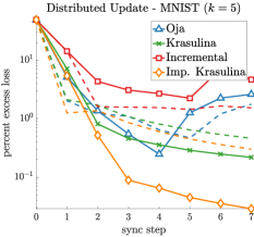
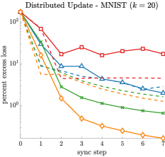
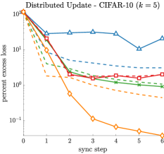
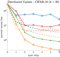
Figure 2: Distributed setting: the results of different algorithms in a distributed setting. The value of $k$ is shown on top of each figure. The updates are carried out across $M=10$ machines and the models are combined and propagated back every $1000$ iterations. The average loss of the machines for each algorithm is shown with a dashed line. The loss of the combined model is shown with a solid line. Note that our implicit Krasulina update consistently improves over time by combining the partial model. The remamining methods are less stable and provide poor results.

Method	MNIST		CIFAR10
	$k=5$	$k=20$	$k=5$	$k=20$
Batch PCA	$35.16$	$18.74$	$86.98$	$48.65$
Single	$37.17\pm 0.01$	$18.77\pm 0.02$	$87.01\pm 0.00$	$48.74\pm 0.04$
Parallel	$35.17\pm 0.00$	$18.77\pm 0.01$	$87.02\pm 0.00$	$48.76\pm 0.04$

Table 2: Loss of the optimal algorithm (i.e. batch PCA) and the loss of the implicit Krasulina algorithm obtained by running on a single machine vs. running in parallel ($M=10$).

Sensitivity to Initial Learning Rate

We demonstrate the sensitivity of each algorithm to the choice of initial learning rate by applying each algorithm using the optimal learning rate (obtained based on the performance on a validation set) as well as the results of running the same algorithm with $0.1\times$ and $10\times$ the optimal learning rate value. We show the results in Table 1. In the table, we show the final loss of each algorithm on the full dataset. Note that the incremental algorithm is unaffected since no learning rate is used for this method. Among the other methods, our implicit Krasulina algorithm provides excellent convergence even with the non-optimal learning rate and has the lowest sensitivity. The performance of Oja’s and Krasulina’s algorithms immediately deteriorates as the value of the learning rate is altered.

Distributed Setting

Finally, we evaluate the results of different algorithms in a distributed setting. We randomly split the data across $M=10$ machines and perform synchronous updates by combining the results every 1000 iterations. In our experiments all $M$ sub-problems have the same size and we use $\alpha_{i}=\nicefrac{{1}}{{M}}$. We propagate back the value of the combined matrix to each machine. For our proposed algorithm, we apply the online EM framework (?) which corresponds to averaging the learned matrices of all machines as in (17). For all the remaining methods, since there exists no clear procedure for combining orthonormal matrices, we naïvely apply the same procedure. However, the average of a set of orthonormal matrices does not necessarily correspond to an orthonormal matrix. Thus, we apply the QR step on the combined matrix before calculating the loss and propagating back the combined value. We show the results in Figure 2. In the figure, we plot the percentage of the excess loss w.r.t. to the loss of the optimal algorithm, i.e. batch PCA. The solid line indicates the performance of the combined model. We also calculate the loss of each individual model (of each machine) on the full dataset over time and plot the average loss value across the machines with a dashed line. This verifies that whether the combined model performs better than each individual model on average.

As can be seen from the figure, our implicit Krasulina algorithm consistently provides excellent performance and converges to the optimal solution. Among the remaining methods, Krasulina’s algorithm provides better convergence behaviour, but converges to an inferior solution. The Oja algorithm as well as the incremental algorithm fail to provide comparable results. The final loss of the combined model for our algorithm is also very close to the final loss of running our algorithm on a single machine on the full dataset, as shown in Table 2.

Conclusion

The advantage of using future gradients has now appeared in a large variety of contexts (e.g. (?; ?; ?)). Here we develop a partially implicit version of Krasulina’s update for the centered $k$-PCA problem that is dramatically better than the standard explicit update. A second key component is to use a latent variable interpretation of the problem and then apply the online EM framework for combining models in a distributed setting (?). Combining sub-models is equally important for the $k$-PCA problem, and finding further practical applications of this second component and blending it with other methods is a promising future direction.

References

- [Allen-Zhu and Li 2017] Allen-Zhu, Z., and Li, Y. 2017. First efficient convergence for streaming k-pca: a global, gap-free, and near-optimal rate. In 2017 IEEE 58th Annual Symposium on Foundations of Computer Science (FOCS), 487–492. IEEE.
- [Amid and Warmuth 2019] Amid, E., and Warmuth, M. K. 2019. Divergence-based motivation for online EM and combining hidden variable models. arXiv preprint arXiv:1902.04107 https://arxiv.org/pdf/1902.04107.pdf.
- [Arora et al. 2012] Arora, R.; Cotter, A.; Livescu, K.; and Srebro, N. 2012. Stochastic optimization for PCA and PLS. In 2012 50th Annual Allerton Conference on Communication, Control, and Computing (Allerton), 861–868. IEEE.
- [Arora, Cotter, and Srebro 2013] Arora, R.; Cotter, A.; and Srebro, N. 2013. Stochastic optimization of PCA with capped MSG. In Advances in Neural Information Processing Systems, 1815–1823.
- [Balsubramani, Dasgupta, and Freund 2013] Balsubramani, A.; Dasgupta, S.; and Freund, Y. 2013. The fast convergence of incremental PCA. In Advances in Neural Information Processing Systems, 3174–3182.
- [Chen, Hua, and Yan 1998] Chen, T.; Hua, Y.; and Yan, W.-Y. 1998. Global convergence of Oja’s subspace algorithm for principal component extraction. IEEE Transactions on Neural Networks 9(1):58–67.
- [Cheng et al. 2007] Cheng, L.; Schuurmans, D.; Wang, S.; Caelli, T.; and Vishwanathan, S. 2007. Implicit online learning with kernels. In Schölkopf, B.; Platt, J. C.; and Hoffman, T., eds., Advances in Neural Information Processing Systems 19. MIT Press. 249–256.
- [Dempster, Laird, and Rubin 1977] Dempster, A. P.; Laird, N. M.; and Rubin, D. B. 1977. Maximum likelihood from incomplete data via the EM algorithm. Journal of the royal statistical society. Series B (methodological) 1–38.
- [Golub and Van Loan 2012] Golub, G. H., and Van Loan, C. F. 2012. Matrix computations, volume 3. JHU press.
- [Halko, Martinsson, and Tropp 2011] Halko, N.; Martinsson, P.-G.; and Tropp, J. A. 2011. Finding structure with randomness: Probabilistic algorithms for constructing approximate matrix decompositions. SIAM review 53(2):217–288.
- [Hassibi, Sayed, and Kailath 1996] Hassibi, B.; Sayed, A. H.; and Kailath, T. 1996. H∞ optimality of the LMS algorithm. IEEE Transactions on Signal Processing 44(2):267–280.
- [Hastie, Tibshirani, and Friedman 2009] Hastie, T.; Tibshirani, R.; and Friedman, J. 2009. The Elements of Statistical Learning – Data Mining, Inference, and Prediction. Springer Series in Statistics.
- [Jain et al. 2016] Jain, P.; Jin, C.; Kakade, S. M.; Netrapalli, P.; and Sidford, A. 2016. Streaming PCA: Matching matrix Bernstein and near-optimal finite sample guarantees for Oja’s algorithm. In Conference on learning theory, 1147–1164.
- [Jolliffe 2011] Jolliffe, I. 2011. Principal component analysis. Springer.
- [Kivinen and Warmuth 1997] Kivinen, J., and Warmuth, M. K. 1997. Exponentiated gradient versus gradient descent for linear predictors. Inf. Comput. 132(1):1–63.
- [Kivinen, Warmuth, and Hassibi 2006] Kivinen, J.; Warmuth, M. K.; and Hassibi, B. 2006. The p-norm generalization of the LMS algorithm for adaptive filtering. IEEE Transactions on Signal Processing 54(5):1782–1793.
- [Krasulina 1969] Krasulina, T. 1969. The method of stochastic approximation for the determination of the least eigenvalue of a symmetrical matrix. USSR Computational Mathematics and Mathematical Physics 9(6):189–195.
- [Kulis and Bartlett 2010] Kulis, B., and Bartlett, P. L. 2010. Implicit online learning. In ICML.
- [Liu, So, and Wu 2016] Liu, H.; So, A. M.-C.; and Wu, W. 2016. Quadratic optimization with orthogonality constraint: explicit Łojasiewicz exponent and linear convergence of retraction-based line-search and stochastic variance-reduced gradient methods. In ICML, 1158–1167.
- [Meyer 1973] Meyer, Jr, C. D. 1973. Generalized inversion of modified matrices. SIAM Journal on Applied Mathematics 24(3):315–323.
- [Nesterov 1983] Nesterov, Y. E. 1983. A method for solving the convex programming problem with convergence rate of (). Dokl. akad. nauk Sssr 269:543–547.
- [Nie, Kotłowski, and Warmuth 2016] Nie, J.; Kotłowski, W.; and Warmuth, M. K. 2016. Online PCA with optimal regret. The Journal of Machine Learning Research 17(1):6022–6070.
- [Oja 1982] Oja, E. 1982. Simplified neuron model as a principal component analyzer. Journal of mathematical biology 15(3):267–273.
- [Pearson 1901] Pearson, K. 1901. LIII. On lines and planes of closest fit to systems of points in space. The London, Edinburgh, and Dublin Philosophical Magazine and Journal of Science 2(11):559–572.
- [Petersen and Pedersen 2008] Petersen, K. B., and Pedersen, M. S. 2008. The matrix cookbook, volume 7(15). Technical University of Denmark. Version 20081110.
- [Roweis 1998] Roweis, S. T. 1998. EM algorithms for PCA and SPCA. In Advances in neural information processing systems, 626–632.
- [Shamir 2015] Shamir, O. 2015. A stochastic PCA and SVD algorithm with an exponential convergence rate. In International Conference on Machine Learning, 144–152.
- [Tang 2019] Tang, C. 2019. Exponentially convergent stochastic k-PCA without variance reduction. arXiv preprint arXiv:1904.01750 https://arxiv.org/abs/1904.01750.
- [Tipping and Bishop 1999] Tipping, M. E., and Bishop, C. M. 1999. Probabilistic principal component analysis. Journal of the Royal Statistical Society: Series B (Statistical Methodology) 61(3):611–622.
- [Van Der Maaten, Postma, and Van den Herik 2009] Van Der Maaten, L.; Postma, E.; and Van den Herik, J. 2009. Dimensionality reduction: a comparative. Journal of Machine Learning Research.
- [Warmuth and Kuzmin 2008] Warmuth, M. K., and Kuzmin, D. 2008. Randomized online PCA algorithms with regret bounds that are logarithmic in the dimension. Journal of Machine Learning Research 9(Oct):2287–2320.
- [Woodbury 1950] Woodbury, M. A. 1950. Inverting Modified Matrices. Princeton, NJ: Department of Statistics, Princeton University.