Unified $\ell_{2\rightarrow\infty}$ Eigenspace Perturbation Theory for Symmetric Random Matrices

Abstract

Modern applications in statistics, computer science and network science have seen tremendous values of finer matrix spectral perturbation theory. In this paper, we derive a generic $\ell_{2\rightarrow\infty}$ eigenspace perturbation bound for symmetric random matrices, with independent or dependent entries and fairly flexible entry distributions. In particular, we apply our generic bound to binary random matrices with independent entries or with certain dependency structures, including the unnormalized Laplacian of inhomogenous random graphs and $m$-dependent matrices. Through a detailed comparison, we found that for binary random matrices with independent entries, our $\ell_{2\rightarrow\infty}$ bound is tighter than all existing bounds that we are aware of, while our eigen-gap condition is weaker than all but one of them in a less common regime. We employ our perturbation bounds in three problems and improve the state of the art: concentration of the spectral norm of sparse random graphs, exact recovery of communities in stochastic block models and partial consistency of divisive hierarchical clustering. Finally we discuss the extensions of our theory to random matrices with more complex dependency structures and non-binary entries, asymmetric rectangular matrices and induced perturbation theory in other metrics.

1 Introduction

Matrix spectral perturbation theory is one of the most fundamental and powerful tool in various areas including statistics, network sciences and computer sciences. In many problems, it is important to understand how eigenvalues and eigenvectors change when the underlying matrix $A^{*}$ is perturbed into $A$. Focusing on symmetric matrices, Weyl’s inequality provides a simple bound for eigenvalues (Weyl, 1912) and Davis-Kahan Theorem provides a surprisingly clean bound for eigenspaces in terms of any unitarily invariant norm (Davis and Kahan, 1970). We refer to interested readers to Stewart (1990), Kato (2013) and the appendix of Bai and Silverstein (2010) for fruitful results over the past century.

Modern applications are posing new challenges for this long-standing area. In these problems, the unitarily invariant norm, such as Frobenius norm or operator norm, in the classical eigenvector perturbation theory may be too coarse to achieve the goal. It is then crucial to derive eigenvector/eigenspace perturbation bounds in terms of finer norms that are not unitarily invariant. Among others, one important norm is the $\ell_{2\rightarrow\infty}$ norm, which yields the row-wise perturbation bound on the eigenvector matrix. To be specific, let $A$ and $A^{*}$ be two symmetric matrices with

$$E=A-A^{*}.$$ (1)

Let $\lambda_{1}\geq\lambda_{2}\geq\ldots\geq\lambda_{n}$ and $\lambda_{1}^{*}\geq\lambda_{2}^{*}\geq\ldots\geq\lambda_{n}^{*}$ be the eigenvalues of $A$ and $A^{*}$, respectively. Given positive integers $s$ and $r$, let

$$\Lambda=\mathrm{diag}(\lambda_{s+1},\lambda_{s+2},\ldots,\lambda_{s+r}),\quad\Lambda^{*}=\mathrm{diag}(\lambda_{s+1}^{*},\lambda_{s+2}^{*},\ldots,\lambda_{s+r}^{*}).$$ (2)

Let $U,U^{*}\in\mathbb{R}^{n\times r}$ be a matrix of eigenvectors such that

$$AU=U\Lambda,\quad A^{*}U^{*}=U^{*}\Lambda^{*}.$$ (3)

The $\ell_{2\rightarrow\infty}$ perturbation theory is seeking for bounds on the $\ell_{2\rightarrow\infty}$ distance between $U$ and $U^{*}$, defined as

$$d_{2\rightarrow\infty}(U,U^{*})\triangleq\inf_{O\in\mathbb{R}^{r\times r},O^{T}O=I}\|UO-U^{*}\|_{2\rightarrow\infty}.$$

where $\|V\|_{2\rightarrow\infty}=\max_{i\in[n]}\|V_{i}\|_{2}$ and $V_{i}$ is the $i$-th row of $V$. The $\ell_{2\rightarrow\infty}$ norm is not invariant to left unitary transformation and thus not supported by classical Davis-Kahan Theorem. When $r=1$, $d_{2\rightarrow\infty}(U,U^{*})$ reduces to the entrywise perturbation of the eigenvector. Compared to perturbation bounds in operator norm, it provides much finer information.

1.1 Existing works

Early efforts on $\ell_{2\rightarrow\infty}$ perturbation was motivated by the stability of Markov chain (e.g. O’cinneide, 1993; Ipsen and Meyer, 1994). The focus was on the stationary distribution, which is the first eigenvector of the transition matrix of a finite state Markov chain. The investigation in random graph theory can be dated back to Mitra (2009) which studied the entrywise perturbation for the leading eigenvector of the adjacency matrix of an Erdös-Rényi graph $\mathbb{G}(n,p)$. In particular, Mitra (2009) considered the sparse graph regime allowing the parameter $p$ to decay with $n$ as long as $p\geq(\log n)^{6}/n$. He further studied the entrywise perturbation of the second eigenvector for dense planted partition models where the within-block average degree is $\sqrt{n}$. This is the first work proving that spectral clustering can achieve exact recovery, namely zero mis-classification error, with high probability. These two lines of works typify two perspectives: the former assumes a non-random $A$ and studies the deterministic perturbation bound, as in Davis-Kahan Theorem, which yields the worst-case guarantee; the latter assumes a stochastic model for $A$ and studies the high probability perturbation bound that is average-case in nature. The deterministic perturbation theory can be applied to more settings, including the stochastic settings, though it is typically much weaker than those stochastic bounds which are tailored to particular random structure.

Recent years has seen a surge of interest in $\ell_{2\rightarrow\infty}$ perturbation theory especially for random matrices. This includes robust covariance estimation and robust principal component analysis for heavy-tailed data (Fan et al., 2018), community detection (Balakrishnan et al., 2011; Eldridge et al., 2017; Mao et al., 2017; Abbe et al., 2017; Cape et al., 2019a), multiple graph inference (Cape et al., 2019b), phase synchronization (Zhong and Boumal, 2018; Abbe et al., 2017), matrix completion (Abbe et al., 2017). It also serves as a powerful tool to push forward other theoretical works such as random graph theory (e.g. Lugosi et al., 2018).

	full	top-$r$	partial	$np^{*}$	$r$	$\kappa^{*}$	$\|U^{*}\|_{2\rightarrow\infty}$
Abbe et al. (2017)	✓	✓	✓	$\succeq\log n/\log\log n$	No	$\preceq\log(np^{*})$	No
Eldridge et al. (2017)	✓	✓	✓	$\succeq(\log n)^{2+\epsilon}$	$=1$	$=1$	$\preceq 1/\sqrt{n}$
Mao et al. (2017)	✓	✗	✗	$\succeq(\log n)^{2+\epsilon}$	No	No	$\preceq\sqrt{rp^{*}}$
Fan et al. (2018)	✓	✓*	✗	$\succeq\log n$	$\preceq 1$	No	$\preceq 1/\sqrt{n}$
Cape et al. (2019a)	✓	✗	✗	$\succeq(\log n)^{2+\epsilon}$	$\preceq(\log n)^{2+\epsilon}$	$\preceq 1$	No
Cape et al. (2019b)	✓	✓*	✗	$\succeq\log n$	No	No	No
This paper	✓	✓	✓	$\succeq\log n/\log\log n$	No	No	No

Table 1: The regime that each method works on for binary random matrices with independent entries. The ✓* symbol in the third column means that the bound is derived for both full and top-$r$ eigenspace recovery but only the former is available for binary random matrices. $p^{*}$ denotes the maximum entry of $A^{*}$ and $\kappa^{*}$ denotes the condition number of $\Lambda^{*}$. The constraints may not be explicitly mentioned in those papers but can be derived from their conditions. They are only necessary conditions and the real constraint may be more stringent. See Appendix E for details.

Despite the great success in different applications, the existing $\ell_{2\rightarrow\infty}$ perturbation theory is not satisfactory in that the bounds work under rather different regimes. To better describe each work, we classify the applicability into three categories:

• Full eigenspace recovery: $s=0$ and $\lambda_{r+1}^{*}=\ldots=\lambda_{n}^{*}=0$. In this case, $A^{*}$ has to be low rank.

• Top-$r$ eigenspace recovery: $s=0$ and there is no restriction on other eigenvalues.

• Partial eigenspace recovery: There is no restriction on $s$ or other eigenvalues.

We consider binary random matrices with independent entries for illustration. Table 1 summarizes the necessary conditions for each bound to work, where $p^{*}$ denotes the maximum entry of $A^{*}$, $\kappa^{*}=\lambda_{s+1}^{*}/\lambda_{s+r}^{*}$ denotes the condition number of $\Lambda^{*}$, and $\preceq(\succeq)$ denotes smaller (larger) in order. See Appendix E for the derivation of these claims. As with Davis-Kahan theorem, $\ell_{2\rightarrow\infty}$ perturbation theory also requires sufficient eigen-gap. Since these bounds work under different regimes, we consider the intersection of them for comparison, namely the regime $np^{*}\succeq(\log n)^{2+\epsilon},r\preceq 1,\kappa^{*}\preceq 1,\|U^{*}\|_{2\rightarrow\infty}\preceq 1/\sqrt{n}$. To simplify we also assume that all entries of $A^{*}$ are in the same order of $p^{*}$. Table 2 summarizes the conditions on eigen-gaps as well as the bounds for each work in this special case.

From Table 1, we can see that the bounds of Eldridge et al. (2017); Mao et al. (2017); Cape et al. (2019a) require the maximum degree $np^{*}$ to grow faster than $(\log n)^{2+\epsilon}$. However, the critical regime of $np^{*}$ in random graph theory is typically $\log n$, under which phase transition occurs. Therefore, although $(\log n)^{2+\epsilon}$ appears to be close to the critical regime, the extra $(\log n)^{1+\epsilon}$ term is too artificial to explain interesting phenomena. Abbe et al. (2017)’s work is the first to remove this extra logarithmic terms using an ingenious leave-one-out argument. Nonetheless, it imposes a stringent assumption on the condition number: in the critical regime it only allows the condition number to grow as $\log\log n$. The bound of Fan et al. (2018) also removes the artificial log-factors but it requires the number of eigenvectors to be bounded and the eigenvectors have low coherence. From Table 2, we can see that all works require a stringent assumption on the eigen-gap except Mao et al. (2017). Indeed, it is easy to show that the eigen-gap is always upper bounded by $np^{*}$. As a consequence, the four works except Mao et al. (2017) require the eigen-gap to be nearly the largest achievable value even in this special regime. By contrast, in Davis-Kahan Theorem, the lower bound on the eigen-gap is simply the operator norm of the perturbation, which is of order $\sqrt{np^{*}}$ in this case. Although Mao et al. (2017) gets rid of the $np^{*}$ lower bound, it still involves extra log-factors. Finally, in terms of the perturbation bound, we see that the bounds of Abbe et al. (2017), Fan et al. (2018) and Cape et al. (2019b) stay the same as $np^{*}$ increases. They are clearly inferior to the others that are decaying with $np^{*}$.

The real problems may not lie in the nice intersection regime as above. The existing bounds work in different regimes and there is no one dominating all others in terms of either applicability or tightness. This creates hurdles to choose which bound to use. Furthermore, it provides evidence that none of the existing bounds is tight and there is still much room for improvement and unification.

	condition on the eigen-gap	$\sqrt{n}d_{2\rightarrow\infty}(U,U^{*})$
Abbe et al. (2017)	$\succeq np^{*}/\log(np^{*})$	$\preceq 1$
Eldridge et al. (2017)	$\succeq np^{*}$	$\preceq\sqrt{(\log n)^{2+\epsilon}/np^{*}}$
Mao et al. (2017)	$\succeq\sqrt{np^{*}}(\log n)^{1+\epsilon/2}$	$\preceq\sqrt{(\log n)^{2+\epsilon}/np^{*}}$
Fan et al. (2018)	$\succeq np^{*}$	$\preceq 1$
Cape et al. (2019a)	$\succeq np^{*}$	$\preceq\sqrt{(\log n)^{2+\epsilon}/np^{*}}$
Cape et al. (2019b)	$\succeq np^{*}$	$\preceq 1$
This paper	$\succeq\sqrt{np^{*}}$	$\preceq\sqrt{\log n/np^{*}}$

Table 2: Comparison of the conditions on the eigen-gap and the bounds in each work under the regime $np^{*}\succeq(\log n)^{2+\epsilon},r\preceq 1,\kappa^{*}\preceq 1,\|U^{*}\|_{2\rightarrow\infty}\preceq 1/\sqrt{n},A_{ij}^{*}\sim p^{*}$.

1.2 This paper

In this paper, we derive generic $d_{2\rightarrow\infty}$ bounds that work for random matrices with independent entries or with dependent entries with certain dependency structures (Theorem 2.3 - Theorem 2.6). As with Abbe et al. (2017) and Cape et al. (2019a), our theory not only covers $d_{2\rightarrow\infty}(U,U^{*})$ but also covers $d_{2\rightarrow\infty}(U,U^{*}+V)$ for some $V\in\mathbb{R}^{n\times r}$ that yields a better approximation of $U$. In our theory, the entry distribution can be arbitrary provided that some characteristics of the perturbation $E$ can be controlled, e.g. operator norm and linear contrasts of rows. This includes but not limited to Bernoulli, Gaussian, sub-Gaussian and sub-exponential distributions. For the sake of length, we only discuss binary random matrices, because it is arguably the most challenging yet most common case calling for $\ell_{2\rightarrow\infty}$ perturbation theory, and provide a brief discussion in Section 7.2 for other entry distributions.

For binary random matrices, we derive the $d_{2\rightarrow\infty}$ bounds for the case with independent entries, or equivalently the adjacency matrix of random graphs (Theorem 3.4). In this case, our bound works in a broader regime than all of existing bounds as shown in the last row of Table 1. Under the special regime for Table 2, our result has the least stringent condition on the eigen-gap that matches Davis-Kahan Theorem while our bound is strictly sharper than all others. Through a more detailed comparison in Appendix E, we found that our bound is tighter than all existing bounds that we are aware of in all regimes, except in some corner cases where our bound is equivalent to some of the others. In addition, our eigen-gap condition is weaker than all others except in the case of full eigenspace recovery with $np^{*}\succeq(\log n)^{2+\epsilon}$, $\min\{\kappa^{*},r\}\succeq(\log n)^{1+\epsilon/2}$ for which Mao et al. (2017)’s condition is weaker than ours.

In addition, we derive the inequality for unnormalized Laplacian of random graphs (Theorem 3.11) and discuss the case for binary matrices with certain $m$-dependence structure (Section 7.1). The former is particularly useful for community detection problems in network science. Both cases are straightforward applications of our generic bounds.

Our bounds can be applied to the problems considered in the works listed in Table 1. In this paper, we apply our bounds to three other problems. The first one is to bound the variance and derive the concentration of the spectral norm of sparse random graphs. This is a fundamental and long-standing problem in random graph theory. Classical theory shows that, for Erdös-Rényi graphs, the variance is bounded by a universal constant regardless of the graph sparsity and the spectral norm is sub-gaussian with an $O(1)$ parameter. The recent work by Lugosi et al. (2018) drastically improves the bound of variance and sub-gaussian parameters to $O(p^{*})$ for Erdös-Rényi graphs using the $\ell_{2\rightarrow\infty}$ perturbation theory. However, they only prove the result for $p^{*}\succeq(\log n)^{3}/n$ and conjecture that it carries over to the critical regime $p^{*}\succeq\log n/n$. We prove this conjecture using our new $\ell_{2\rightarrow\infty}$ perturbation theory. Moreover, we extend the result to general inhomogeneous random graphs.

The second problem is the strong consistency of spectral clustering for community detection in sparse stochastic block models (SBM). Despite the substantial literature on this topic, existing algorithms are rarely as easy-to-implement and computationally efficient as the standard spectral clustering algorithm (e.g. Von Luxburg, 2007), which is simply a singular value decomposition plus a $K$-means algorithm. However, perhaps surprisingly, the strong consistency of spectral clustering in sparse graphs is not established until recently (Abbe et al., 2017; Su et al., 2019). In this paper, we apply our $\ell_{2\rightarrow\infty}$ bounds to prove the strong consistency of spectral clustering algorithms, using the adjacency matrix or the unnormalized Laplacian, for general SBMs in the critical regime with average degree $O(\log n)$. We also study the SBMs with growing number of communities and obtain the best available dependence on it for spectral algorithms.

The third problem is the partial consistency of divisive hierarchical clustering on binary tree stochastic block models (BTSBM), proposed by Li et al. (2018a). BTSBMs are special SBMs that embed communities into a tree-like hierarchy in order to bring interpretability. It is also a useful framework to analyze divisive hierarchical clustering algorithms such as iterative spectral bi-partitioning (e.g. Spielman and Teng, 1996; Balakrishnan et al., 2011). Li et al. (2018a) derived sufficient conditions that certain divisive hierarchical clustering algorithms are able to exactly recover the whole or a part of the hierarchy in the regime with the average degree $O((\log n)^{2+\epsilon})$. In this paper, we extend the result to the critical regime where each connection can be written as $a_{j}\log n/n$ and establish the sufficient condition to recover any part of the hierarchy in terms of the coefficients $a_{j}$’s. We found an unexpected connection between BTSBMs and mis-specified SBMs. In addition we accurately quantify an observation in Li et al. (2018a) that certain partial structure may still be recovered even if the communities are information theoretically unrecoverable.

The rest of the article is organized as follows: Section 2 presents the generic bounds and Section 3 presents the bounds for binary random matrices. Three examples are collected in Section 4 - Section 6. Section 7 discusses several extensions, including binary random matrices with $m$-dependence structure, random matrices with non-binary entry distribution, singular space perturbation for asymmetric matrices and perturbation bounds in other metrics. Most technical proofs are relegated into Appendix. Appendix A establishes the proof of our main generic bound. The proof is quite involved so we parse it into six steps. All other proofs related to the generic bounds are presented in Appendix B. Appendix C contains all technical proofs for binary random matrices. The miscellaneous proofs in Section 4 - Section 6 are collected in Appendix D. Appendix E provides a detailed comparison between our bounds and all existing ones that we are aware of. This includes the justification of Table 1 and Table 2. Finally, Appendix F presents useful concentration inequalities for binary random variables which are useful in Section 3.

2 An Generic $\ell_{2\rightarrow\infty}$ Bound for Symmetric Random Matrices

2.1 Notations and assumptions

Throughout the paper we consider the setup 1 - 3. We denote by $[n]$ the set $\{1,\ldots,n\}$ and by $\textbf{1}_{n}$ the $n$-dimensional vector with all entries $1$. For any vector $x$, let $\|x\|_{p}$ denotes its $p$-norm. For any matrix $M$, let $M_{k}^{T}$ denote the $m$-th row of $M$, $\|M\|_{\mathrm{op}}$ denote its operator norm and $\|M\|_{\mathrm{F}}$ denote its Frobenius norm. When $M$ is a square matrix, we define the matrix sign as

$$\mathrm{sign}(M)=UV^{T}.$$

By definition, $\mathrm{sign}(M)$ is orthogonal. When $n=1$, $M$ is a scalar and $\mathrm{sign}(M)$ reduces to the classical sign of scalars. Further we denote by $\lambda_{\max}(M)$ (resp. $\lambda_{\min}(M)$) the largest (resp. the smallest) eigenvalue of $M$ in absolute values, by $\kappa(M)$ the condition number $\lambda_{\max}(M)/\lambda_{\min}(M)$. In particular we write $\lambda_{\min}^{*}(\Lambda^{*})$ as $\lambda_{\min}^{*}$ for short.

To state our generic bound, we need to define the following quantities.

• Effective eigen-gap $\Delta^{*}$:

  $$\Delta^{*}\triangleq\min\{\mathrm{sep}_{s+1,s+r}(A^{*}),\lambda_{\min}^{*}\},$$ (4)

  where $\mathrm{sep}_{s+1,s+r}(A^{*})=\min\{\lambda_{s}^{*}-\lambda_{s+1}^{*},\lambda_{s+r}^{*}-\lambda_{s+r+1}^{*}\}$ with $\lambda_{0}^{*}=\infty$ and $\lambda_{n+1}^{*}=-\infty$. Note that $\Delta^{*}=\mathrm{sep}_{s+1,s+r}(A^{*})$ except when $\Lambda^{*}$ includes both positive and negative eigenvalues but $0$ is not an eigenvalue of $\Lambda^{*}$. Therefore $\Delta^{*}$ is essentially the eigen-gap in the conventional sense.

• Effective condition number $\bar{\kappa}^{*}$:

  $$\bar{\kappa}^{*}\triangleq\min\{\kappa(\Lambda^{*}),2r\},$$ (5)

  Note that the effective condition number is never larger $2r$ however ill-conditioned the problem is. On the other hand, if $\Lambda^{*}$ is well-conditioned but $r$ is large, $\bar{\kappa}^{*}$ can also be small.

• full eigenspace $\bar{U}^{*}$ of $A^{*}$, i.e.

  $$A^{*}\bar{U}^{*}=\bar{U}^{*}\bar{\Lambda^{*}},$$ (6)

  where $\bar{\Lambda}^{*}$ includes all non-zero eigenvalues of $A^{*}$. Note that the number of columns $\bar{U}^{*}$ may significantly differ from that of $U^{*}$;

Our generic $\ell_{2\rightarrow\infty}$ bound requires the following four assumptions.

1. For any $\delta\in(0,1)$, there exists a random matrix $A^{(k)}\in\mathbb{R}^{n\times n}$ such that

   $$d_{TV}(\mathbb{P}_{(A_{k},A^{(k)})},\mathbb{P}_{A_{k}}\times\mathbb{P}_{A^{(k)}})\leq\delta/n,$$ (7)

   where $d_{TV}$ denotes the total variation distance and it holds simultaneously for all $k$ and all contiguous subsets $S\subset[r]$ that

   $$\|A^{(k)}-A\|_{\mathrm{op}}\leq L_{1}(\delta),\quad\frac{\|(A^{(k)}-A)U_{S}\|_{\mathrm{op}}}{\lambda_{\min}(\Lambda_{S}^{*})}\leq\left(\kappa(\Lambda_{S}^{*})L_{2}(\delta)+L_{3}(\delta)\right)\|U_{S}\|_{2\rightarrow\infty},$$

   with probability at least $1-\delta$ for some deterministic functions $L_{1}(\delta),L_{2}(\delta),L_{3}(\delta)$, where $U_{S}\in\mathbb{R}^{n\times|S|}$ denotes the matrix formed by columns of $U$ with indices in $S$.

2. There exists deterministic functions $\lambda_{-}(\delta),E_{+}(\delta),\bar{E}_{+}(\delta),E_{\infty}(\delta)$, such that for any $\delta\in(0,1)$, the following event occurs with probability at least $1-\delta$:

   $$\|\Lambda-\Lambda^{*}\|_{\max}\leq\lambda_{-}(\delta),\quad\|EU^{*}\|_{\mathrm{op}}\leq E_{+}(\delta),\quad\|E\bar{U}^{*}\|_{\mathrm{op}}\leq\bar{E}_{+}(\delta),\quad\|E\|_{2\rightarrow\infty}\leq E_{\infty}(\delta).$$

3. There exist deterministic functions $b_{\infty}(\delta),b_{2}(\delta)>0$, such that for any $\delta\in(0,1)$, $k\in[n]$, $r^{\prime}\leq r$ and fixed matrix $W\in\mathbb{R}^{n\times r^{\prime}}$,

   $$\|E_{k}^{T}W\|_{2} \leq b_{\infty}(\delta)\|W\|_{2\rightarrow\infty}+b_{2}(\delta)\|W\|_{\mathrm{op}},\,\,\mbox{with probability at least }1-\delta/n,$$

4. $\Delta^{*}\geq 4\left(\sigma(\delta)+L_{1}(\delta)+\lambda_{-}(\delta)\right)$ where

   $$\eta(\delta)=E_{\infty}(\delta)+b_{\infty}(\delta)+b_{2}(\delta),\quad\sigma(\delta)=\{\bar{\kappa}^{*}L_{2}(\delta)+L_{3}(\delta)+1\}\eta(\delta)+E_{+}(\delta),$$ (8)

Assumption A1 is worth some discussion. Roughly speaking, A1 controls the amount and the structure of entry dependence. The following proposition gives three cases where $L_{1}(\delta),L_{2}(\delta)$ and $L_{3}(\delta)$ can be exactly characterized. The proof is relegated to Appendix B.

Proposition 2.1.

Assume that

1. If $A_{ij}$’s are independent random variables, then there exists $A^{(k)}$ such that A1 is satisfied with

   $$L_{1}(\delta)=\sqrt{2}(\|A^{*}\|_{2\rightarrow\infty}+E_{\infty}(\delta)),\quad L_{2}(\delta)=1,\quad L_{3}(\delta)=\frac{E_{\infty}(\delta)+\lambda_{-}(\delta)+\|A^{*}\|_{2\rightarrow\infty}}{\lambda_{\min}^{*}}.$$

2. Assume that for any $k$, there exists a subset $\mathcal{N}_{k}\subset[n]$, such that $A_{k}$ is independent of $\{A_{i}:i\not\in\mathcal{N}_{k}\}$. Let $m=\max_{k}|\mathcal{N}_{k}|$, then there exists $A^{(k)}$ such that A1 is satisfied with

   $$L_{1}(\delta)=\sqrt{2m}(\|A^{*}\|_{2\rightarrow\infty}+E_{\infty}(\delta)),\quad L_{2}(\delta)=m,\quad L_{3}(\delta)=\frac{m(E_{\infty}(\delta)+\lambda_{-}(\delta)+\|A^{*}\|_{2\rightarrow\infty})}{\lambda_{\min}^{*}}.$$

In literature (e.g. Abbe et al., 2017), it is typically assumed that

$$\|E\|_{\mathrm{op}}\leq E_{2}(\delta)\quad\mbox{with probability at least }1-\delta.$$ (9)

Assumption A2 is satisfied under 9 if

$$\lambda_{-}(\delta)=E_{+}(\delta)=\bar{E}_{+}(\delta)=E_{\infty}(\delta)=E_{2}(\delta).$$ (10)

This is because $\|\Lambda-\Lambda^{*}\|_{\max}\leq\|E\|_{\mathrm{op}}$ by Weyl’s inequality, $\|EU^{*}\|_{\mathrm{op}}\leq\|E\|_{\mathrm{op}},\|E\bar{U}^{*}\|_{\mathrm{op}}\leq\|E\|_{\mathrm{op}}$ and $\|E\|_{2\rightarrow\infty}\leq\|E\|_{\mathrm{op}}$ by definition. In general, A2 can be strictly weaker than 9.

Assumption A3 requires a concentration inequality on linear transforms of rows of $E$. A similar version is consisdered in Abbe et al. (2017) except that the operator norm is replaced by the Frobenius norm. We emphasize that our assumption A3 can yield tighter result when $r>1$. Using a standard $\epsilon$-net argument, A3 can be verified by considering vectors $W$ only. The following proposition summarizes the result with the proof relegated to Appendix C.

Proposition 2.2.

Suppose that for any $\delta\in(0,1)$ and vector $w\in\mathbb{R}^{n}$, there exists $a_{\infty}(\delta),a_{2}(\delta)>0$ such that for each $k$

$$E_{k}^{T}w \leq a_{\infty}(\delta)\|w\|_{\infty}+a_{2}(\delta)\|w\|_{2},$$

with probability at least $1-\delta$. Then assumption A3 holds with

$$b_{\infty}(\delta)=2a_{\infty}\left(\frac{\delta}{5^{r}n}\right),\quad b_{2}(\delta)=2a_{2}\left(\frac{\delta}{5^{r}n}\right).$$

Assumption A4 guarantees sufficient eigen-gap. In classical perturbation theory (e.g. Davis and Kahan, 1970) based on operator norm or Frobenius norm, it is necessary to assume $\Delta^{*}\succeq\lambda_{-}(\delta)$. Nonetheless, we will show that A4 is equivalent to $\Delta^{*}\succeq\lambda_{-}(\delta)$ in many applications.

2.2 Main results

Based on our assumptions, we first derive an bound for $d_{2\rightarrow\infty}(U,AU^{*}(\Lambda^{*})^{-1})$. As shown in Abbe et al. (2017) and Cape et al. (2019b), $AU^{*}(\Lambda^{*})^{-1}$ is a better approximation of $U$ than $U^{*}$. The proof is quite involved and thus presented step by step in Appendix A.

Theorem 2.3.

Given any $\delta\in(0,1)$. Let $\Delta^{*},\bar{\kappa}^{*}$ and $\bar{U}^{*}$ be defined in 4 - 6. Then under assumptions A1-A4,

$$d_{2\rightarrow\infty}(U,AU^{*}(\Lambda^{*})^{-1}) \leq\frac{C}{\Delta^{*}}\bigg{\{}\sigma(\delta)\left(\|U^{*}\|_{2\rightarrow\infty}+\frac{\|EU^{*}\|_{2\rightarrow\infty}}{\lambda_{\min}^{*}}\right)+\frac{E_{+}(\delta)b_{2}(\delta)}{\lambda_{\min}^{*}}$$

$$\qquad\quad+\min\left\{E_{+}(\delta)\xi_{1},\bar{E}_{+}(\delta)\sqrt{\bar{\kappa}^{*}}\xi_{2},\bar{E}_{+}(\delta)\bar{\kappa}^{*}\xi_{3}\right\}\bigg{\}},$$

with probability at least $1-B(r)\delta$, where $C$ is a universal constant (that can be chosen as $72$),

$$B(r)=10\min\{r,1+\log_{2}\kappa^{*}\},$$ (11)

and

$$\xi_{1}=\frac{\|A^{*}\|_{2\rightarrow\infty}}{\lambda_{\min}^{*}},\quad\xi_{2}=\frac{\sqrt{\|A^{*}\|_{\max}}}{\sqrt{\lambda_{\min}^{*}}I(A^{*}\mbox{ is psd})},\quad\xi_{3}=\|\bar{U}^{*}\|_{2\rightarrow\infty}.$$ (12)

Remark 2.1.

The last term is the minimum of three fundamentally different bounds, which are obtained from Kato’s integral (e.g. Kato, 1949); see Appendix A.4 for details. The second term kicks in only when $A^{*}$ is postive semi-definite. This is true in many cases such as spiked wigner ensemble and phase synchronization (e.g. Abbe et al., 2017). The third term becomes useful for full eigenspace recovery. This is common in the cases of community detection (Section 5).

Remark 2.2.

All terms in the bound are deterministic except for $\|EU^{*}\|_{2\rightarrow\infty}$. Although assumption A3 directly yields a bound as follows:

$$\|EU^{*}\|_{2\rightarrow\infty}\leq b_{\infty}(\delta)\|U^{*}\|_{2\rightarrow\infty}+b_{2}(\delta)\|U^{*}\|_{\mathrm{op}}=b_{\infty}(\delta)\|U^{*}\|_{2\rightarrow\infty}+b_{2}(\delta),$$

we found it can be sharpened in some applications; see Section 3 for instance. For this reason we keep this term in the bound and derive its upper tail case by case.

Remark 2.3.

Recall that $d_{2\rightarrow\infty}(U,AU^{*}(\Lambda^{*})^{-1})=\inf_{O\in\mathbb{R}^{r\times r},O^{T}O=I}\|UO-AU^{*}(\Lambda^{*})^{-1}\|_{2\rightarrow\infty}$. In our proof, we find a particular orthogonal matrix $\tilde{O}$ such that the proved bound holds for $\|U\tilde{O}-AU^{*}(\Lambda^{*})^{-1}\|_{2\rightarrow\infty}$. Indeed, this orthogonal matrix is in the form of

$$\tilde{O}=\mathrm{diag}(\mathrm{sign}(U_{1}^{T}U_{1}^{*}),\ldots,\mathrm{sign}(U_{J}^{T}U_{J}^{*}))$$

where $U_{1},\ldots,U_{J}$ (resp. $U_{1}^{*},\ldots,U_{J}^{*}$) form a partition of $U$ (resp. $U^{*}$) and the eigenvalues corresponding to each $U_{j}$ (resp. $U_{j}^{*}$) consist of consecutive eigenvalues in $\Lambda$ (resp. $\Lambda^{*}$). Furthermore, as shown in Step I-IV in Appendix A, Theorem 2.3 holds for $\|U\mathrm{sign}(U^{T}U^{*})-AU^{*}(\Lambda^{*})^{-1}\|_{2\rightarrow\infty}$ if $\bar{\kappa}^{*}$ is replaced by $\kappa^{*}$, in both the assumptions and the bound. This also applies to Theorem 2.4 - 2.6.

By the triangle inequality, we can directly obtain the following perturbation bound for $d_{2\rightarrow\infty}(U,U^{*})$ by $d_{2\rightarrow\infty}(U,AU^{*}(\Lambda^{*})^{-1})+d_{2\rightarrow\infty}(AU^{*}(\Lambda^{*})^{-1},U^{*})$. We leave the proof in Appendix B. In many cases, the first term dominates the second term, in which cases Theorem 2.4 essentially implies that $d_{2\rightarrow\infty}(U,U^{*})\asymp\|EU^{*}\|_{2\rightarrow\infty}/\lambda_{\min}^{*}$.

Theorem 2.4.

Under the same setting of Theorem 2.3,

$$d_{2\rightarrow\infty}(U,U^{*})\leq\frac{C\|EU^{*}\|_{2\rightarrow\infty}}{\lambda_{\min}^{*}}$$

$$+\frac{C}{\Delta^{*}}\bigg{\{}\sigma(\delta)\|U^{*}\|_{2\rightarrow\infty}+\frac{E_{+}(\delta)b_{2}(\delta)}{\lambda_{\min}^{*}}+\min\left\{E_{+}(\delta)\xi_{1},\bar{E}_{+}(\delta)\sqrt{\bar{\kappa}^{*}}\xi_{2},\bar{E}_{+}(\delta)\bar{\kappa}^{*}\xi_{3}\right\}\bigg{\}},$$

with probability at least $1-B(r)\delta$, where $C$ is a universal constant (that can be chosen as $72$).

2.3 Sharpening the bound via diagonal surgery

In this subsection we discuss a trick, referred to as “diagonal surgery”, to further improve the $\ell_{2\rightarrow\infty}$ bound. The motivation is from matrices with large diagonal elements. If $A^{*}$ has high rank or even full rank, the last term in Theorem 2.3 and 2.4 reduce to $\min\{\xi_{1},\sqrt{\bar{\kappa}^{*}}\xi_{2}\}$. However, both $\xi_{1}$ and $\xi_{2}$ will be large when $A^{*}$ has large diagonal elements. For instance, when $A$ is the unnormalized graph Laplacian, defined in Section 3.2 later, of an Erdös-Renyi graph with edge connection probability $p$, then $\|A^{*}\|_{2\rightarrow\infty}\geq\|A^{*}\|_{\max}=(n-1)p$. By contrast, when $A$ is the adjacency matrix, $\|A^{*}\|_{2\rightarrow\infty}=p\sqrt{n-1},\|A^{*}\|_{\max}=p$. If we had used Theorem 2.3 or 2.4, the bound applied to graph Laplacian would be significantly worse than that applied to the adjacency matrix. To overcome this shortcoming, we found a modification of the proof that allows us to replace $A$ by $A-\Sigma$ where $\Sigma$ is a possibly random diagonal matrix, provided that all diagonal elements of $\Sigma$ are well separated from $\Lambda^{*}$. This trick was implicitly used in Balakrishnan et al. (2011). Specifically, we need the following assumption:

1. For any $\delta\in(0,1)$,

   $$\frac{\min_{j\in[s+1,s+r]}|\Lambda_{jj}^{*}|}{\min_{j\in[s+1,s+r],k\in[n]}|\Lambda_{jj}^{*}-\Sigma_{kk}|}\leq\Theta(\delta),$$

   with probability at least $1-\delta$ for some deterministic function $\Theta(\delta)>0$.

Let

$$\tilde{A}=A-\Sigma,\quad\tilde{A}^{*}=\mathbb{E}\tilde{A},\quad\tilde{E}=\tilde{A}-\tilde{A}^{*}.$$ (13)

All other assumptions need to be slightly modified.

1. The same as A1 except that 7 is replaced by

   $$d_{TV}\left(\mathbb{P}_{(\tilde{E}_{k},A^{(k)})},\mathbb{P}_{\tilde{E}_{k}}\times\mathbb{P}_{A^{(k)}}\right)\leq\delta/n.$$

2. There exists deterministic functions $\lambda_{-}(\delta),E_{+}(\delta),\tilde{E}_{\infty}(\delta)$, such that for any $\delta\in(0,1)$, the following event holds with probability at least $1-\delta$:

   $$\|\Lambda-\Lambda^{*}\|_{\max}\leq\lambda_{-}(\delta),\quad\|EU^{*}\|_{\mathrm{op}}\leq E_{+}(\delta),\quad\|\tilde{E}\|_{2\rightarrow\infty}\leq\tilde{E}_{\infty}(\delta).$$

3. There exists deterministic functions $\tilde{b}_{\infty}(\delta),\tilde{b}_{2}(\delta)>0$, such that for any $\delta\in(0,1)$, $k\in[n]$, $r^{\prime}\leq r$ and fixed matrix $W\in\mathbb{R}^{n\times r^{\prime}}$,

   $$\|\tilde{E}_{k}^{T}W\|_{2} \leq\tilde{b}_{\infty}(\delta)\|W\|_{2\rightarrow\infty}+\tilde{b}_{2}(\delta)\|W\|_{\mathrm{op}},\,\,\mbox{with probability at least }1-\delta/n.$$

4. $\Delta^{*}\geq 4\left(\Theta(\delta)\tilde{\sigma}(\delta)+L_{1}(\delta)+\lambda_{-}(\delta)+E_{+}(\delta)\right)$ where

   $$\tilde{\eta}(\delta)=\tilde{E}_{\infty}(\delta)+\tilde{b}_{\infty}(\delta)+\tilde{b}_{2}(\delta),\quad\tilde{\sigma}(\delta)=\{\bar{\kappa}^{*}L_{2}(\delta)+L_{3}(\delta)+1\}\tilde{\eta}(\delta)+E_{+}(\delta).$$ (14)

Unlike Theorem 2.3, $AU^{*}(\Lambda^{*})^{-1}$ is no longer an approximation of $U$ after “diagonal surgery”. In fact, the approximation becomes $U^{*}+V$ where

$$V_{k}^{T}=E_{k}^{T}U^{*}(\Lambda^{*}-\Sigma_{kk}I)^{-1}.$$ (15)

Note that when $\Sigma_{kk}\equiv 0$,

$$U^{*}+V=U^{*}+EU^{*}(\Lambda^{*})^{-1}=AU^{*}(\Lambda^{*})^{-1},$$

which recovers the case in Section 2.2.

Theorem 2.5.

Given any $\delta\in(0,1)$. Let $\Delta^{*}$ be defined in 4 and $\bar{\kappa}^{*}$ be defined in 5. Then under assumptions A’0 - A’4,

$$d_{2\rightarrow\infty}(U,U^{*}+V) \leq C\bigg{\{}\left(\frac{E_{+}^{2}(\delta)}{(\Delta^{*})^{2}}+\frac{\Theta(\delta)\tilde{\sigma}(\delta)}{\Delta^{*}}\right)\left(\|U^{*}\|_{2\rightarrow\infty}+\frac{\Theta(\delta)\|EU^{*}\|_{2\rightarrow\infty}}{\lambda_{\min}^{*}}\right)$$

$$\qquad\quad+\frac{\Theta(\delta)(\tilde{b}_{2}(\delta)+\|\tilde{A}^{*}\|_{2\rightarrow\infty})E_{+}(\delta)}{\lambda_{\min}^{*}\Delta^{*}}\bigg{\}},$$

with probability at least $1-B(r)\delta$, where $B(r)$ is defined in 11 and $C$ is a universal constant (that can be chosen as $136$).

Similar to Theorem 2.4, we can derive a bound for $d_{2\rightarrow\infty}(U,U^{*})$ using the triangle inequality.

Theorem 2.6.

Under the same setting of Theorem 2.5,

$$d_{2\rightarrow\infty}(U,U^{*}) \leq C\bigg{\{}\frac{\Theta(\delta)}{\lambda_{\min}^{*}}\|EU^{*}\|_{2\rightarrow\infty}+\left(\frac{E_{+}^{2}(\delta)}{(\Delta^{*})^{2}}+\frac{\Theta(\delta)\tilde{\sigma}(\delta)}{\Delta^{*}}\right)\|U^{*}\|_{2\rightarrow\infty}$$

$$\qquad\quad+\frac{\Theta(\delta)(\tilde{b}_{2}(\delta)+\|\tilde{A}^{*}\|_{2\rightarrow\infty})E_{+}(\delta)}{\lambda_{\min}^{*}\Delta^{*}}\bigg{\}},$$

with probability at least $1-B(r)\delta$, where $C$ is a universal constant (that can be chosen as $136$).

3 $\ell_{2\rightarrow\infty}$ Perturbation Theory for Binary Random Matrices

Throughout this section we will ignore the universal constant terms for notational convenience. In particular, we use the symbol $\preceq$ (resp. $\succeq$) to hide universal constants. We say a constant is universal if it does not depend on any quantity in the problem (e.g. $A^{*}$, $n$, $\delta$, etc.). Specifically, we say $A\preceq B$ (resp. $A\succeq B$) with probability $1-\delta$ for two variables $A$ and $B$, stochastic or deterministic, if and only if $A\leq CB$ (resp. $A\geq CB$) with probability $1-\delta$ for some universal constant $C$. All proofs in this section are relegated to Appendix C.

3.1 Binary random matrices with independent entries

In this subsection, we consider $A$ as a binary random matrix with independent entries with $A^{*}$ being its expectation, i.e.

$$A_{ij}^{*}=A_{ji}^{*}=p_{ij},\quad A_{ij}=A_{ji}\sim\mathrm{Ber}(p_{ij}),\quad(A_{ij})_{1\leq i\leq j\leq n}\mbox{ are independent}.$$ (16)

Note that we allow $p_{ii}>0$. Let

$$p^{*}=\max_{ij}p_{ij},\quad\bar{p}^{*}=\max_{i}\frac{1}{n}\sum_{j=1}^{n}p_{ij},\quad R(\delta)=\log(n/\delta)+r.$$ (17)

Lemma 3.1.

Under the setting 16, given any $\alpha>0$, assumption A3 is satisfied with

$$b_{\infty}(\delta)\preceq\frac{R(\delta)}{\alpha\log R(\delta)},\quad b_{2}(\delta)\preceq\frac{\sqrt{p^{*}}R(\delta)^{(1+\alpha)/2}}{\alpha\log R(\delta)}.$$

Lemma 3.2.

Under the setting 16, assumption A2 is satisfied with

$$\lambda_{-}(\delta),E_{+}(\delta),\bar{E}_{+}(\delta),E_{\infty}(\delta)\preceq\sqrt{n\bar{p}^{*}}+\sqrt{\log(n/\delta)},$$

Lemma 3.3.

Under the setting 16, with probability $1-\delta$,

$$\|EU^{*}\|_{2\rightarrow\infty}\preceq R(\delta)\|U^{*}\|_{2\rightarrow\infty}+\sqrt{R(\delta)p^{*}}.$$

It is then easy to derive the $\ell_{2\rightarrow\infty}$ perturbation theory for binary random matrices with independent entries from Theorem 2.3 and 2.4 based on Lemma 3.1 - 3.3 and Proposition 2.1 on $L_{1}(\delta),L_{2}(\delta),L_{3}(\delta)$.

Theorem 3.4.

Fix any $\delta\in(0,1),\alpha\in(0,1)$. Let

$$g(\delta)=\sqrt{n\bar{p}^{*}}+\frac{R(\delta)}{\alpha\log R(\delta)},$$ (18)

and assume that

$$\Delta^{*}\geq C\bar{\kappa}^{*}g(\delta),$$ (19)

for some universal constant $C$ that is large enough. Then with probability at least $1-(B(r)+1)\delta$,

$$d_{2\rightarrow\infty}(U,AU^{*}(\Lambda^{*})^{-1})\preceq\frac{1}{\Delta^{*}}\left\{\bar{\kappa}^{*}g(\delta)\left(1+\frac{R(\delta)}{\lambda_{\min}^{*}}\right)\|U^{*}\|_{2\rightarrow\infty}+\frac{\sqrt{R(\delta)p^{*}}}{\lambda_{\min}^{*}}\left(\bar{\kappa}^{*}g(\delta)+\frac{\sqrt{n\bar{p}^{*}R(\delta)^{\alpha}}}{\alpha\log R(\delta)}\right)\right\}$$

$$\,\,+\frac{\sqrt{n\bar{p}^{*}}+\sqrt{\log(n/\delta)}}{\Delta^{*}}\min\left\{\frac{\|A^{*}\|_{2\rightarrow\infty}}{\lambda_{\min}^{*}},\frac{\sqrt{\bar{\kappa}^{*}p^{*}}}{\sqrt{\lambda_{\min}^{*}}I(A^{*}\mbox{ is psd})},\bar{\kappa}^{*}\|\bar{U}^{*}\|_{2\rightarrow\infty}\right\},$$

and

$$d_{2\rightarrow\infty}(U,U^{*})\preceq\left(\frac{\bar{\kappa}^{*}g(\delta)}{\Delta^{*}}+\frac{R(\delta)}{\lambda_{\min}^{*}}\right)\|U^{*}\|_{2\rightarrow\infty}+\frac{\sqrt{R(\delta)p^{*}}}{\lambda_{\min}^{*}}\left(1+\frac{\sqrt{n\bar{p}^{*}R(\delta)^{\alpha}}}{\alpha\Delta^{*}\log R(\delta)}\right)$$

$$\,\,+\frac{\sqrt{n\bar{p}^{*}}+\sqrt{\log(n/\delta)}}{\Delta^{*}}\min\left\{\frac{\|A^{*}\|_{2\rightarrow\infty}}{\lambda_{\min}^{*}},\frac{\sqrt{\bar{\kappa}^{*}p^{*}}}{\sqrt{\lambda_{\min}^{*}}I(A^{*}\mbox{ is psd})},\bar{\kappa}^{*}\|\bar{U}^{*}\|_{2\rightarrow\infty}\right\},$$

We consider two special but realistic cases where the bounds in Theorem 3.4 can be significantly simplified. The first case corresponds to the full eigenspace recovery. This is a widely studied problem in various areas such as community detection. We will discuss a few applications in Section 5. The following Corollary considers a slightly more general case where $\bar{U}^{*}$ can differ from $U^{*}$. In this case the last terms in both inequalities can be removed.

Corollary 3.5.

Under the settings of Theorem 3.4, if

$$\|\bar{U}^{*}\|_{2\rightarrow\infty}\preceq\|U^{*}\|_{2\rightarrow\infty},$$

then with probability at least $1-(B(r)+1)\delta$,

$$d_{2\rightarrow\infty}(U,AU^{*}(\Lambda^{*})^{-1}) \preceq\frac{1}{\Delta^{*}}\bigg{\{}\bar{\kappa}^{*}g(\delta)\left(1+\frac{R(\delta)}{\lambda_{\min}^{*}}\right)\|U^{*}\|_{2\rightarrow\infty}+\frac{\sqrt{R(\delta)p^{*}}}{\lambda_{\min}^{*}}\left(\bar{\kappa}^{*}g(\delta)+\frac{\sqrt{n\bar{p}^{*}R(\delta)^{\alpha}}}{\alpha\log R(\delta)}\right)\bigg{\}},$$

$$d_{2\rightarrow\infty}(U,U^{*}) \preceq\left(\frac{\bar{\kappa}^{*}g(\delta)}{\Delta^{*}}+\frac{R(\delta)}{\lambda_{\min}^{*}}\right)\|U^{*}\|_{2\rightarrow\infty}+\frac{\sqrt{R(\delta)p^{*}}}{\lambda_{\min}^{*}}\left(1+\frac{\sqrt{n\bar{p}^{*}R(\delta)^{\alpha}}}{\alpha\Delta^{*}\log R(\delta)}\right).$$

The second case we consider imposes a lower bound for $\lambda_{\min}^{*}$.

Corollary 3.6.

Under the settings of Theorem 3.4, if

$$\lambda_{\min}^{*}\succeq\frac{np^{*}}{\sqrt{n}\|U^{*}\|_{2\rightarrow\infty}},$$ (20)

then with probability at least $1-(B(r)+1)\delta$,

$$d_{2\rightarrow\infty}(U,AU^{*}(\Lambda^{*})^{-1}) \preceq\frac{\bar{\kappa}^{*}g(\delta)}{\Delta^{*}}\left(1+\frac{R(\delta)}{\lambda_{\min}^{*}}\right)\|U^{*}\|_{2\rightarrow\infty},$$

$$d_{2\rightarrow\infty}(U,U^{*}) \preceq\left(\frac{\bar{\kappa}^{*}g(\delta)}{\Delta^{*}}+\frac{R(\delta)}{\lambda_{\min}^{*}}\right)\|U^{*}\|_{2\rightarrow\infty}+\frac{\sqrt{R(\delta)p^{*}}}{\lambda_{\min}^{*}}.$$

3.2 Unnormalized graph laplacian

Let $\mathcal{A}$ be a binary matrix with independent entries as defined in 16 and $\mathcal{L}$ be the unnormalized graph Laplacian of $\mathcal{A}$,

$$\mathcal{L}=\mathcal{D}-\mathcal{A},\quad\mbox{where }\mathcal{D}=\mathrm{diag}(D_{11},\ldots,D_{nn}),\quad\mathcal{D}_{ii}=\sum_{j=1}^{n}\mathcal{A}_{ij}.$$ (21)

We use the notation $\mathcal{L},\mathcal{D},\mathcal{A}$ by convention. We assume $\mathcal{A}_{ii}=0$ without loss of generality (because $\mathcal{L}$ does not depend on $\mathcal{A}_{ii}$). Throughout this section we will treat $\mathcal{L}$ as $A$ and $\mathcal{L}^{*}$ as $A^{*}$. Similar to binary matrices with independent entries, we derive the bound for quantities involved in Theorem 2.3. In particular, we apply the diagonal surgery technique with $\Sigma=\mathrm{diag}(\mathcal{L}_{11},\mathcal{L}_{22},\ldots,\mathcal{L}_{nn})$. Let

$$\tilde{\mathcal{L}}=\mathcal{L}-\Sigma,\quad E=\mathcal{L}-\mathbb{E}\mathcal{L},\quad\tilde{E}=\tilde{\mathcal{L}}-\mathbb{E}\tilde{\mathcal{L}}.$$

Apart from the notation in 17, we also define the following quantity

$$M(\delta)=\sqrt{n\bar{p}^{*}\log(n/\delta)}+\log(n/\delta).$$ (22)

Lemma 3.7.

Under the setting 21, given any $\alpha>0$, assumption A’3 is satisfied with

$$\tilde{b}_{\infty}(\delta)\preceq\frac{R(\delta)}{\alpha\log R(\delta)},\quad\tilde{b}_{2}(\delta)\preceq\frac{\sqrt{p^{*}}R(\delta)^{(1+\alpha)/2}}{\alpha\log R(\delta)}.$$

Lemma 3.8.

Under the setting 21, assumption A’2 is satisfied with

$$\tilde{E}_{\infty}(\delta)\preceq\sqrt{n\bar{p}^{*}}+\sqrt{\log(n/\delta)},\quad E_{+}(\delta),\lambda_{-}(\delta)\preceq M(\delta).$$

Lemma 3.9.

Under the setting 21, with probability $1-\delta$,

$$\|EU^{*}\|_{2\rightarrow\infty}\preceq(M(\delta)+r)\|U^{*}\|_{2\rightarrow\infty}+\sqrt{R(\delta)p^{*}}.$$

Lemma 3.10.

Let $\mathcal{L}$ be the unnormalized Laplacian of $\mathcal{A}$ where $\mathcal{A}$ is a binary random matrix that satisfies the condition in part (b) of Proposition 2.1. Then there exists $\mathcal{L}^{(1)},\ldots,\mathcal{L}^{(n)}$ satisfying A’1 with

$$L_{1}(\delta)\preceq\sqrt{m}M(\delta)+m(\sqrt{n\bar{p}^{*}}+\sqrt{\log(n/\delta)}),\quad L_{2}(\delta)=m,\quad L_{3}(\delta)\preceq\frac{m\left(n\bar{p}^{*}+\log(n/\delta)\right)}{\lambda_{\min}^{*}}.$$

In particular, the setting considered in this subsection is a special case with $m=1$. Putting the pieces together we deduce the following theorem.

Theorem 3.11.

Fix any $\delta\in(0,1)$ and $\alpha>0$. Let $R(\delta)$, $g(\delta)$ and $M(\delta)$ be defined as in 17, 18 and 22, respectively. Further let

$$\bar{\kappa}^{\prime}=\bar{\kappa}^{*}+n\bar{p}^{*}/\lambda_{\min}^{*},$$

and assume that

$$\Delta^{*}\geq C\{\Theta(\delta)\bar{\kappa}^{\prime}g(\delta)+(\Theta(\delta)+1)M(\delta)\},$$ (23)

for some universal constant $C$ that is large enough. Then with probability at least $1-(B(r)+1)\delta$,

$$d_{2\rightarrow\infty}(U,U^{*}+V) \preceq\left(\frac{M(\delta)^{2}}{(\Delta^{*})^{2}}+\frac{\Theta(\delta)(\bar{\kappa}^{\prime}g(\delta)+M(\delta))}{\Delta^{*}}\right)\left\{\left(1+\frac{\Theta(\delta)r}{\lambda_{\min}^{*}}\right)\|U^{*}\|_{2\rightarrow\infty}+\frac{\Theta(\delta)\sqrt{R(\delta)p^{*}}}{\lambda_{\min}^{*}}\right\}$$

$$\quad+\frac{\Theta(\delta)M(\delta)\sqrt{p^{*}}}{\Delta^{*}\lambda_{\min}^{*}}\left(\sqrt{n\bar{p}^{*}}+\frac{\sqrt{R(\delta)^{1+\alpha}}}{\alpha\log R(\delta)}\right),$$

and

$$d_{2\rightarrow\infty}(U,U^{*}) \preceq\left(\frac{M(\delta)^{2}}{(\Delta^{*})^{2}}+\frac{\Theta(\delta)(\bar{\kappa}^{\prime}g(\delta)+M(\delta))}{\Delta^{*}}+\frac{\Theta(\delta)r}{\lambda_{\min}^{*}}\right)\|U^{*}\|_{2\rightarrow\infty}+\frac{\Theta(\delta)\sqrt{Rp^{*}}}{\lambda_{\min}^{*}}$$

$$\quad+\frac{\Theta(\delta)M(\delta)\sqrt{p^{*}}}{\Delta^{*}\lambda_{\min}^{*}}\left(\sqrt{n\bar{p}^{*}}+\frac{\sqrt{R(\delta)^{1+\alpha}}}{\alpha\log R(\delta)}\right).$$

Note that

$$\frac{|\Lambda^{*}_{jj}|}{|\Lambda^{*}_{jj}-\mathcal{L}_{kk}|}\leq\frac{\Lambda^{*}_{jj}}{\max\{0,|\Lambda^{*}_{jj}-\mathcal{L}^{*}_{kk}|-|\mathcal{L}_{kk}-\mathcal{L}^{*}_{kk}|\}}.$$

It is easy to derive a concentration inequality for $\max_{k}|\mathcal{L}_{kk}-\mathcal{L}^{*}_{kk}|$. This suggests the following bound for $\Theta(\delta)$.

Lemma 3.12.

Let

$$\Theta^{*}=\frac{\min_{j\in[s+1,s+r]}|\Lambda^{*}_{jj}|}{\min_{j\in[s+1,s+r],k\in[n]}|\Lambda^{*}_{jj}-\mathcal{L}^{*}_{kk}|}.$$ (24)

Then $\Theta(\delta)\leq 5\Theta^{*}$ if

$$\min_{j\in[s+1,s+r],k\in[n]}|\Lambda^{*}_{jj}-\mathcal{L}^{*}_{kk}|\geq 5M(\delta).$$

4 Concentration of The Spectral Norm of Random Graphs

4.1 Background

Erdös-Rényi graph is the most fundamental object in random graph theory. The probability connection matrix $A^{*}$ of an Erdös-Rényi graph has

$$A_{ii}^{*}=0,\quad A_{ij}^{*}=p,\quad\forall i\not=j.$$

Concentration of the spectral norm or the extreme eigenvalues of Erdös-Rényi graphs has received considerable attention. Adapted from the proof of Boucheron et al. (2013) (Example 3.14), based on Efron-Stein inequality, we can show that

$$\operatorname*{Var}(\|A\|_{\mathrm{op}})\leq 2.$$ (25)

Alon et al. (2002) proved the sub-gaussian behavior of $\|A\|_{\mathrm{op}}$ in the sense that

$$\mathbb{P}(|\|A\|_{\mathrm{op}}-\mathbb{E}\|A\|_{\mathrm{op}}|>t)\leq 2e^{-t^{2}/32},\quad\forall t>0.$$ (26)

See also (Boucheron et al., 2013, Example 8.7) for a simplified proof. The key argument underlying the above results is the Efron-Stein-type inequalities that involve the leave-one-out behavior of $\|A\|_{\mathrm{op}}$ as a function of independent random variables $(A_{ij})_{i<j}$. Specifically, write $\|A\|_{\mathrm{op}}$ as $Z$ for convenience and denote by $Z_{ij}$ the operator norm of matrix $A^{(ij)}$, which equals to $A$ except that the $(i,j)$-th entry is replaced by an independent copy $A_{ij}^{\prime}$ drawn from a Bernoulli distribution with parameter $p$. Then Efron-Stein inequality implies that

$$\operatorname*{Var}(Z)\leq\mathbb{E}V_{+},\quad\mbox{where }V_{+}=\mathbb{E}^{\prime}\sum_{i<j}(Z-Z_{ij})_{+}^{2}.$$ (27)

Here $(x)_{+}$ denotes $\max\{x,0\}$ by convention and $\mathbb{E}^{\prime}$ denotes the expectation over $(A_{ij}^{\prime})_{i<j}$ (while conditioning on $(A_{ij})_{i<j}$). Using the variational representation of operator norm, we can rewrite $Z-Z_{ij}$ as follows:

$$Z-Z_{ij}=\sup_{u:\|u\|=1}|u^{T}Au|-\sup_{u:\|u\|=1}|u^{T}A^{(ij)}u|.$$

Let $u_{1}$ be the eigenvector of $A$ corresponding to its largest eigenvalue in absolute values, then

$$\sup_{u:\|u\|=1}|u^{T}Au|=\|A\|_{\mathrm{op}},\quad\sup_{u:\|u\|=1}|u^{T}A^{(ij)}u|\geq|u_{1}^{T}A^{(ij)}u_{1}|\geq\pm u_{1}^{T}A^{(ij)}u_{1}.$$

If $u_{1}^{T}Au_{1}\geq 0$, then

$$Z-Z_{ij}\leq u_{1}^{T}(A-A^{(ij)})u_{1}\leq|u_{1}^{T}(A-A^{(ij)})u_{1}|;$$

if $u_{1}^{T}Au_{1}<0$, then

$$Z-Z_{ij}\leq-u_{1}^{T}(A-A^{(ij)})u_{1}\leq|u_{1}^{T}(A-A^{(ij)})u_{1}|.$$

Putting two pieces together, we conclude that

$$(Z-Z_{ij})_{+}\leq|u_{1}^{T}(A-A^{(ij)})u_{1}|=2|u_{1i}||u_{1j}||A_{ij}-A_{ij}^{\prime}|.$$ (28)

As a result,

$$V_{+}\leq 4\sum_{i<j}u_{1i}^{2}u_{1j}^{2}\mathbb{E}^{\prime}(A_{ij}-A_{ij}^{\prime})^{2}=4\sum_{i<j}u_{1i}^{2}u_{1j}^{2}(p+(1-2p)A_{ij}).$$ (29)

To prove 25, one can simply use the naive bound that

$$p+(1-2p)A_{ij}\leq p+1-2p\leq 1.$$

Therefore, we obtain an almost sure bound for $V_{+}$:

$$V_{+}\leq 4\sum_{i<j}u_{1i}^{2}u_{1j}^{2}=2\sum_{i\not=j}u_{1i}^{2}u_{1j}^{2}\leq 2\left(\sum_{i=1}^{n}u_{1i}^{2}\right)^{2}=2.$$ (30)

Then Efron-Stein inequality implies that

$$\operatorname*{Var}(\|A\|_{\mathrm{op}})\leq\mathbb{E}V_{+}\leq 2.$$

However, this bound is loose for small $p$ in which case the term $(p+(1-2p)A_{ij})$ is most likely equal to $p$ instead of the conservative bound $1$. However, the complicated dependence between $u_{1}$ and $A$ makes it hard to operationalize this intuition. Recently, an interesting work by Lugosi et al. (2018) showed that

$$\operatorname*{Var}(\|A\|_{\mathrm{op}})\leq c_{1}p,\quad\mbox{if }p\geq c_{2}(\log n)^{3}/n.$$ (31)

for some universal constant $c_{1},c_{2}>0$. Furthermore, they proved the partial sub-gaussian behavior of $\|A\|_{\mathrm{op}}$ in the sense that

$$\mathbb{P}(|\|A\|_{\mathrm{op}}-\mathbb{E}\|A\|_{\mathrm{op}}|>\sqrt{p}t)\leq c_{3}e^{-t^{2}/c_{4}},\quad\forall t\leq c_{5}\sqrt{np}\log(np)/(\log n\log(1/p)),$$ (32)

for some universal constants $c_{3},c_{4},c_{5}>0$ under the condition that $p\geq c_{2}(\log n)^{3}/n$. Under this regime, the upper bound for $t$ in 32 is diverging, implying that the tail probability holds for values much larger than $\sqrt{p}$.

The idea is based on the phenomenon called ”eigenvector delocalization” that all entries of $u_{1}$ are small (e.g. Mitra, 2009; Erdös et al., 2013; Lugosi et al., 2018). Intuitively, $u_{1}$ should be close to $u_{1}^{*}$, the eigenvector of $A^{*}$ corresponding to the largest eigenvalue in absolute values. A simple calculation shows that $u_{1}^{*}=\textbf{1}_{n}/\sqrt{n}$. In particular, Lugosi et al. (2018) improved the previous results and proved that with high probability, $\|u_{1}\|_{\infty}\preceq 1/\sqrt{n}$ if $p\succeq(\log n)^{3}/n$. This motivates the following bound for $V_{+}$ in 29

$$V_{+}\leq\|u_{1}\|_{\infty}^{4}W,\quad\mbox{where }W=4\sum_{i<j}(p+(1-2p)A_{ij}).$$ (33)

Using the concentration that $\|u\|_{\infty}\approx 1/\sqrt{n}$ and $W\approx\mathbb{E}W=4n(n-1)p(1-p)$ and by Efron-Stein inequality 27, they proved that

$$\operatorname*{Var}(\|A\|_{\mathrm{op}})\leq\mathbb{E}V_{+}\preceq\frac{n(n-1)p(1-p)}{n^{2}}\preceq p.$$

The bound of tail probability in 32 can be derived similarly using higher moments of $V_{+}$ and the moment concentration inequalities derived by Boucheron et al. (2005).

Lugosi et al. (2018) conjectured that the requirement $p\succeq(\log n)^{3}/n$ is artifical and the critical regime should be $p\succeq\log n/n$. In this section, we will close this gap by using our $\ell_{2\rightarrow\infty}$ bound in Section 3.1. Furthermore, we will discuss the behavior of $\|A\|_{\mathrm{op}}$ when $p\preceq\log n/n$ but $p\succeq\log/(n\log\log n)$. Throughout the rest of this section we assume that

$$\frac{1}{2}\geq p\geq\frac{C_{0}\log n}{n\log\log n}$$ (34)

for some universal constant $C_{0}>0$. Similar to Section 3, we use the notation $\preceq$ and $\succeq$ to hide universal constants.

4.2 Improved results for Erdös-Rényi graphs

To start with, we state the moment concentration inequality by Boucheron et al. (2005).

Proposition 4.1 (Theorem 15.6 and 15.7 of Boucheron et al. (2013)).

Let $Z=f(A)$ and $Z_{ij}=f(A^{(ij)})$. Further let $V_{+}$ be defined in 27 and

$$M=\max_{i<j}(Z-Z_{ij})_{+}.$$

Then for any $k\geq 2$,

$$\left(\mathbb{E}(Z-\mathbb{E}Z)_{+}^{k}\right)^{1/k}\leq\sqrt{3k}\left(\mathbb{E}[V_{+}]^{k/2}\right)^{1/k},$$

$$\left(\mathbb{E}(Z-\mathbb{E}Z)_{-}^{k}\right)^{1/k}\leq\sqrt{4.16k}\left\{\left(\mathbb{E}[V_{+}]^{k/2}\right)^{1/k}+\sqrt{k}(\mathbb{E}[M^{k}])^{1/k}\right\}.$$

As a result,

$$(\mathbb{E}|Z-\mathbb{E}Z|^{k})^{1/k}\leq 4\sqrt{k}\left(\mathbb{E}[V_{+}]^{k/2}\right)^{1/k}+4k(\mathbb{E}[M^{k}])^{1/k}.$$

It is well-known (e.g. Vershynin, 2010) that $Z$ is sub-gaussian with parameter $\sigma^{2}$ iff $(\mathbb{E}|Z-\mathbb{E}Z|^{k})^{1/k}\leq c\sqrt{k}\sigma$ for any $k\geq 2$ with some universal constant $c$. Suppose this is true for $k\leq k_{0}$, then we can still derive the sub-gaussian behavior of $Z$.

Lemma 4.2.

If for $2\leq k\leq k_{0}$,

$$(\mathbb{E}|Z-\mathbb{E}Z|^{k})^{1/k}\leq\sqrt{k}\sigma,$$

for some $\sigma>0$, then for $t\leq\sqrt{k_{0}e}\sigma$,

$$\mathbb{P}(|Z-\mathbb{E}Z|\geq t)\leq\exp\left\{1-\frac{t^{2}}{2e\sigma^{2}}\right\}.$$

Although Lemma 4.2 does not hold for all $t$, it is desirable if $k_{0}$ is large because $\sigma$ is the scale of $|Z-\mathbb{E}Z|$. In the following, we will bound the higher order moments of $V_{+}$ and $M$, thereby bounding the tail probability of $\|A\|_{\mathrm{op}}$. Recalling from 28 and 33 that

$$M\leq 2\|u_{1}\|_{\infty}^{2},\quad V_{+}\leq\|u_{1}\|_{\infty}^{4}W.$$

Both involve the moments of $\|u_{1}\|_{\infty}$. Our theory in Section 3 gives the $(1-\delta)$ upper tail bound for $\|u_{1}-u_{1}^{*}\|_{\infty}$ in the form of

$$\mathbb{P}\left(\|u_{1}-u_{1}^{*}\|_{\infty}\geq A_{1}+A_{2}\sqrt{\log\left(\frac{1}{\delta}\right)}+A_{3}\log\frac{1}{\delta}\right)\leq\delta.$$ (35)

If 35 holds for all $\delta$ then it directly yields a moment bound using Fubini’s formula. However, $\delta$ cannot be arbitrarily small otherwise the condition 19 in Theorem 2.3 may be violated so that 35 may fail. So we first characterize the minimal $\delta$ such that 35 remains valid.

Lemma 4.3.

Under condition 34, 19 holds for all $\delta>\delta^{*}$ where

$$\delta^{*}=\exp\left\{-\frac{np\log(np)}{2C}\right\},$$ (36)

and $C$ is the constant in 19 in Theorem 3.4, if $C_{0}$ and $n$ are bounded below by a universal constant (which can be chosen as $\max\{64C^{2},12C,16\}$).

Based on Lemma 4.3 and Corollary 3.6, we can derive the moment bound for $V_{+}$ and $M$.

Lemma 4.4.

Under the assumptions of Lemma 4.3, for any $k>0$,

$$\left(\mathbb{E}V_{+}^{k/2}\right)^{1/k}\preceq\sqrt{p}\left(1+\frac{(k\vee\log n)^{2}}{(np)^{2}}\right)+\exp\left\{-\frac{np\log(np)}{2Ck}\right\},$$

and

$$\left(\mathbb{E}M^{k}\right)^{1/k}\preceq\frac{1}{n}\left(1+\frac{(k\vee\log n)^{2}}{(np)^{2}}\right)+\exp\left\{-\frac{np\log(np)}{2Ck}\right\},$$

where $C$ is the constant in 19 in Theorem 3.4.

Proof.

In this case, note that $A^{*}=p\textbf{1}_{n}\textbf{1}_{n}^{T}-pI_{n\times n}$. Then

$$p^{*}=p,\quad\lambda_{1}^{*}=(n-1)p,\quad\lambda_{2}^{*}=\ldots=\lambda_{n}^{*}=-p,\,\,\mbox{ and }u_{1}^{*}=\textbf{1}_{n}/\sqrt{n}.$$

Let $\Lambda^{*}=\lambda_{1}^{*}$, then

$$\Delta^{*}=\lambda_{\min}^{*}=(n-1)p,\quad\|U^{*}\|_{2\rightarrow\infty}=\|u_{1}^{*}\|_{\infty}=\frac{1}{\sqrt{n}},\quad\bar{\kappa}^{*}=1.$$

Thus,

$$\lambda_{\min}^{*}\succeq\frac{np^{*}}{\sqrt{n}\|U^{*}\|_{2\rightarrow\infty}}.$$

By Lemma 4.3 below, the condition 19 is satisfied for all $\delta\geq\delta^{*}$. Then by Corollary 3.6 with $\alpha=0.5$ and $\delta\geq\delta^{*}$, with probability $1-\delta$,

$$d_{2\rightarrow\infty}(u_{1},u_{1}^{*}) \preceq\left(\frac{\sqrt{np}+\log(n/\delta)/\log\log(n/\delta)}{np}+\frac{\log(n/\delta)}{np}\right)\frac{1}{\sqrt{n}}+\frac{\sqrt{\log(n/\delta)p}}{np}$$

$$\preceq\frac{1}{\sqrt{n}}\left(\frac{\sqrt{np}+\log(n/\delta)/\log\log(n/\delta)}{np}+\frac{\log(n/\delta)}{np}+\sqrt{\frac{\log(n/\delta)}{np}}\right)$$

$$\preceq\frac{1}{\sqrt{n}}\left(\frac{\log(n/\delta)}{np}+\sqrt{\frac{\log(n/\delta)}{np}}\right)$$

By the triangle inequality,

$$\|u_{1}\|_{\infty}\leq d_{2\rightarrow\infty}(u_{1},u_{1}^{*})+\|u_{1}^{*}\|_{\infty}.$$

Using the fact that $2\sqrt{y}\leq y+1$ and $\sqrt{n}\|u_{1}^{*}\|_{\infty}=1$, there exists a universal constant $C_{1}$ such that for each $\delta\geq\delta^{*}$,

$$\sqrt{n}\|u_{1}\|_{\infty}\leq C_{1}\left(1+\frac{\log(n/\delta)}{np}\right)\leq C_{1}\left(1+\frac{\log n}{np}+\frac{\log(1/\delta)}{np}\right),$$ (37)

with probability $1-\delta$. Denote by $B_{u}$ the RHS of 37 with $\delta=\delta^{*}$ and by $\mathcal{V}_{1}$ the event that $\sqrt{n}\|u_{1}\|_{\infty}\leq B_{u}$. Then

$$\mathbb{P}(\mathcal{V}_{1})\geq 1-\delta^{*}=1-\exp\left\{-\frac{np\log(np)}{2C}\right\}.$$

On the other hand, note that

$$\mathbb{E}W=4\sum_{i<j}(p+(1-2p)p)=4n(n-1)p(1-p)\leq 4n^{2}p,$$

and

$$W-\mathbb{E}W=4(1-2p)\sum_{i<j}(A_{ij}-p).$$

By Lemma F.1 with $w=\textbf{1}_{n(n-1)/2}$ and $\delta=\delta^{\prime}=\exp\{-e/2\Omega\}=\exp\{-en(n-1)p/4\}$,

$$W-\mathbb{E}W\leq 8\log\left(\frac{1}{\delta}\right)=2en(n-1)p\leq 6n^{2}p$$

with probability $1-\delta$. Let $\mathcal{V}_{2}$ denote the event that $W\leq 10n^{2}p$, then

$$\mathbb{P}(\mathcal{V}_{2})\geq 1-\exp\{-en(n-1)p/4\}\geq 1-\exp\{-n^{2}p/3\}.$$ (38)

Let $\mathcal{V}=\mathcal{V}_{1}\cup\mathcal{V}_{2}$. Then

$$\mathbb{P}(\mathcal{V}^{c})\leq\exp\left\{-\frac{np\log(np)}{2C}\right\}+\exp\left\{-\frac{n^{2}p}{3}\right\}\leq C_{2}\exp\left\{-\frac{np\log(np)}{2C}\right\},$$

where $C_{2}$ is a universal constant. By definition, on $\mathcal{V}$,

$$\|u_{1}\|_{\infty}^{4}W\leq 10p(\sqrt{n}\|u_{1}\|_{\infty})^{4}.$$

In addition, by 30 we have

$$V_{+}I_{\mathcal{V}^{c}}\leq 2I_{\mathcal{V}^{c}}.$$

Therefore,

$$\left(\mathbb{E}V_{+}^{k/2}\right)^{1/k} =\left(\mathbb{E}V_{+}^{k/2}I_{\mathcal{V}}+\mathbb{E}V_{+}^{k/2}I_{\mathcal{V}^{c}}\right)^{1/k}\leq\left(\mathbb{E}V_{+}^{k/2}I_{\mathcal{V}}\right)^{1/k}+\left(\mathbb{E}V_{+}^{k/2}I_{\mathcal{V}^{c}}\right)^{1/k}$$

$$\preceq\sqrt{p}\mathbb{E}\left(\left[(\sqrt{n}\|u_{1}\|_{\infty})^{2k}I_{\mathcal{V}}\right]\right)^{1/k}+\exp\left\{-\frac{np\log(np)}{2Ck}\right\}$$ (39)

By 37,

$$\mathbb{P}\left(Y\leq\frac{\log(1/\delta)}{np}\right)\leq\delta,\quad\forall\delta\geq\delta^{*},\quad\mbox{where }Y=\left[\frac{\sqrt{n}\|u_{1}\|_{\infty}}{C_{1}}-\left(1+\frac{\log n}{np}\right)\right]_{+}.$$

Denote by $B_{Y}$ the upper bound with $\delta=\delta^{*}$. This can be written equivalently as

$$\mathbb{P}(Y\geq y)\leq\exp\left\{-npy\right\},\quad\forall y\leq B_{Y}.$$

By definition, $YI_{\mathcal{V}}\leq YI(Y\leq B_{Y})$. Using Fubini’s theorem, for any $k>0$,

$$\mathbb{E}Y^{2k}I(Y\leq B_{Y}) =\int_{0}^{B_{Y}}2ky^{2k-1}\mathbb{P}(Y\geq y)dy\leq\int_{0}^{B_{Y}}2ky^{2k-1}\exp\{-npy\}dy$$

$$\leq\int_{0}^{\infty}2ky^{2k-1}\exp\{-npy\}dy=\frac{\Gamma(2k+1)}{(np)^{2k}}.$$

By Stirling’s formula, we have

$$\left(\mathbb{E}Y^{2k}I_{\mathcal{V}}\right)^{1/k}\leq\left(\mathbb{E}Y^{2k}I(Y\leq B_{Y})\right)^{1/k}\preceq\frac{k^{2}}{(np)^{2}}.$$

As a result,

$$\left(\mathbb{E}(\sqrt{n}\|u_{1}\|_{\infty})^{2k}I_{\mathcal{V}}\right)^{1/k}\leq\left(\mathbb{E}\left(C_{1}Y+1+\frac{\log n}{np}\right)^{2k}I_{\mathcal{V}}\right)^{1/k}$$

$$\leq \left(2^{2k}\mathbb{E}\left(C_{1}Y\right)^{2k}I_{\mathcal{V}}+2^{2k}\left(1+\frac{\log n}{np}\right)^{2k}\right)^{1/k}\leq 4C_{1}^{2}\left(\mathbb{E}Y^{2k}I_{\mathcal{V}}\right)^{1/k}+4\left(1+\frac{\log n}{np}\right)^{2}$$

$$\preceq \frac{k^{2}}{(np)^{2}}+1+\frac{(\log n)^{2}}{(np)^{2}}\preceq 1+\frac{(k\vee\log n)^{2}}{(np)^{2}}.$$ (40)

The bound of $\left(\mathbb{E}[V_{+}^{k/2}]\right)^{1/k}$ is then proved by pluggin this into 39.

Recalling 28, we have

$$M\leq 2\|u_{1}\|_{\infty}^{2}.$$

It is easy to see that $M\leq 2$. Similar to 39,

$$\left(\mathbb{E}M^{k}\right)^{1/k} \leq\left(\mathbb{E}M^{k}I_{\mathcal{V}}+\mathbb{E}M^{k/2}I_{\mathcal{V}^{c}}\right)^{1/k}\leq\left(\mathbb{E}M^{k}I_{\mathcal{V}}\right)^{1/k}+\left(\mathbb{E}M^{k}I_{\mathcal{V}^{c}}\right)^{1/k}$$

$$\preceq\frac{1}{n}\mathbb{E}\left(\left[(\sqrt{n}\|u_{1}\|_{\infty})^{2k}I_{\mathcal{V}}\right]\right)^{1/k}+\exp\left\{-\frac{np\log(np)}{2Ck}\right\}.$$ (41)

The bound of $\left(\mathbb{E}M^{k}\right)^{1/k}$ is then completed by 40. ∎

Theorem 4.5.

Under condition 34 with $C_{0}$ sufficiently large,

$$\operatorname*{Var}(\|A\|_{\mathrm{op}})\preceq p\left(1+\frac{(\log n)^{4}}{(np)^{4}}\right).$$

In particular, if $p\succeq\log n/n$, then

$$\operatorname*{Var}(\|A\|_{\mathrm{op}})\preceq p.$$

Remark 4.1.

This closed the gap conjectured by Lugosi et al. (2018). Moreover, our result shows that when $np\sim\log n/\log\log n$,

$$\operatorname*{Var}(\|A\|_{\mathrm{op}})\preceq p(\log\log n)^{4}.$$

Proof.

By Efron-Stein inequality 27,

$$\operatorname*{Var}(\|A\|_{\mathrm{op}})\leq\mathbb{E}V_{+}.$$

For sufficiently large $n$, by Lemma 4.4 with $k=2$,

$$\mathbb{E}V_{+}\leq p\left(1+\frac{(\log n)^{4}}{(np)^{4}}\right)+\exp\left\{-\frac{np\log(np)}{4C}\right\}.$$

Since $np\geq C_{0}\log n/\log\log n$, when $C_{0}$ is sufficiently large,

$$\exp\left\{-\frac{np\log(np)}{4C}\right\}\preceq n^{-2}\preceq p.$$

For small $n$, $\operatorname*{Var}(\|A\|)_{\mathrm{op}}\leq 2$ as shown in 25. In summary,

$$\operatorname*{Var}(\|A\|_{\mathrm{op}})\preceq p\left(1+\frac{(\log n)^{4}}{(np)^{4}}\right).$$

∎

Lemma 4.6.

Under condition 34,

$$\left(\mathbb{E}|Z-\mathbb{E}Z|^{k}\right)^{1/k}\leq C^{\prime}\sqrt{kp}\left(1+\frac{(\log n)^{2}}{(np)^{2}}\right),\quad\forall k\leq k_{0},$$

where $C^{\prime}$ is a universal constant and

$$k_{0}=\frac{np}{2C\vee 1}\min\left\{1,\frac{\log(np)}{\log(1/p)}\right\}.$$ (42)

Proof.

Write $\|A\|_{\mathrm{op}}$ as $Z$ when no confusion can arise. By Proposition 4.1 and Lemma 4.4,

$$(\mathbb{E}|Z-\mathbb{E}Z|^{k})^{1/k}\preceq\left(\sqrt{kp}+\frac{k}{n}\right)\left(1+\frac{(k\vee\log n)^{2}}{(np)^{2}}\right)+k\exp\left\{-\frac{np\log(np)}{2Ck}\right\}.$$

For $k\leq k_{0}$, then the first term has the order of $\sqrt{kp}$ because under 34,

$$\frac{k}{n}=\sqrt{kp}\frac{1}{\sqrt{n^{2}p}}\preceq\sqrt{kp},\quad 1+\frac{(k\vee\log n)^{2}}{(np)^{2}}\preceq 1+\frac{(\log n)^{2}}{(np)^{2}}$$

To bound the second term is dominated by $\sqrt{kp}$ in order, it is left to show that

$$\sqrt{\frac{k}{p}}\exp\left\{-\frac{np\log(np)}{2Ck}\right\}=\exp\left\{-\frac{np\log(np)}{2Ck}+\frac{1}{2}\log k+\frac{1}{2}\log\left(\frac{1}{p}\right)\right\}\preceq 1.$$ (43)

Since $k\leq k_{0}\leq np/(2C\vee 1)$,

$$k\log k\leq\frac{np\log(np)}{2C}\Longrightarrow\log k\leq\frac{np\log(np)}{2Ck}.$$

Further, since $k\leq k_{0}\leq np\log(np)/2C\log(1/p)$,

$$\log\left(\frac{1}{p}\right)\leq\frac{np\log(np)}{2Ck}.$$

Thus,

$$-\frac{np\log(np)}{2Ck}+\frac{1}{2}\log k+\frac{1}{2}\log\left(\frac{1}{p}\right)\leq 0,$$

and 43 is proved. The proof is then completed. ∎

Together with Lemma 4.2, Lemma 4.6 implies that partial sub-gaussian behavior of $\|A\|_{\mathrm{op}}$.

Theorem 4.7.

Under condition 34, there exists universal constants $C_{1},C_{2}>0$ such that

$$\mathbb{P}(|Z-\mathbb{E}Z|\geq t)\leq\exp\left\{1-\frac{t^{2}}{C_{1}\sigma^{2}}\right\},\quad\forall t\leq C_{2}\sigma\sqrt{np}\min\left\{1,\sqrt{\frac{\log(np)}{\log(1/p)}}\right\},$$

where

$$\sigma=\sqrt{p}\left(1+\frac{(\log n)^{2}}{(np)^{2}}\right).$$

Remark 4.2.

When $p\succeq\log n/n$, $\sigma\preceq\sqrt{p}$. This proves the conjecture of Lugosi et al. (2018). On the other hand, it is worth comparing the range of $t$ with the sub-gaussian behaviors. In Lugosi et al. (2018) (equation (2.1)), the multiplicative factor of $\sqrt{p}$ in the upper bound of $t$ is $\sqrt{np}\log(np)/\log n\log(1/p)$ while that of ours is $np\min\{1,\log(np)/\log(1/p)\}$, ignoring the constants. When $np=\mathrm{PolyLog}(n)$, ours reduces to $np\log(np)/\log(1/p)$ which is $\sqrt{np}\log n$ larger than the one in Lugosi et al. (2018).

4.3 Extension to inhomogeneous graphs

The results can be directly extended to general inhomogenous graphs because the proof carries over if both $\|u_{1}-u_{1}^{*}\|_{\infty}$ and $\|u_{1}^{*}\|_{\infty}$ have small moments. To be specific we consider a random graph with an adjacency matrix under the setting of Section 3.1. Apart from $p^{*}$ and $\bar{p}^{*}$ defined in 17, we further defined

$$\bar{p}=\frac{1}{n(n-1)}\sum_{i\not=j}p_{ij}.$$

Note that $\bar{p}\leq\bar{p}^{*}\leq p^{*}$ and in many applications they differ in small multiplicative factors. We distinguish them to cover the cases where many $p_{ij}$’s are tiny. Then we can apply Theorem 3.4 to achieve the task. Here for convenience we assume that $|\lambda_{1}^{*}|\succeq np^{*}/\sqrt{n}\|u_{1}^{*}\|_{\infty}$ so that the simplified bound in Corollary 3.6 can be applied. Further we consider the case with $p^{*}\leq 1/2$ for convenience. The proof is more technical but qualitatively the same as the results for Erdös-Rényi graphs so we present it in Appendix D.1.

Theorem 4.8.

Let $|\lambda_{1}^{*}|\geq|\lambda_{2}^{*}|\geq\ldots\geq|\lambda_{n}^{*}|$ be eigenvalues of $A^{*}$. Suppose $|\lambda_{1}^{*}|>|\lambda_{2}^{*}|$ and let $u_{1}^{*}$ be the eigenvector corresponding to $\lambda_{1}^{*}$. Let

$$\zeta=\sqrt{n}\|u_{1}^{*}\|_{\infty}.$$

Assume that

$$|\lambda_{1}^{*}|\geq C_{0}\frac{np^{*}}{\zeta},\quad\Delta^{*}=\min\left\{|\lambda_{1}^{*}|,\min_{j}|\lambda_{1}^{*}-\lambda_{j}^{*}|\right\}\geq C_{0}\left(\sqrt{n\bar{p}^{*}}+\frac{\log n}{\log\log n}\right),\quad n^{2}\bar{p}\geq C_{0}.$$ (44)

Then

$$\operatorname*{Var}(\|A\|_{\mathrm{op}})\preceq\bar{p}\left\{1+\left(\frac{\sqrt{n\bar{p}^{*}}+\log n}{\Delta^{*}}\right)^{4}\right\}\zeta^{4}+\exp\left\{-\frac{\Delta^{*}\log\Delta^{*}\wedge n^{2}\bar{p}}{2C\vee 3}\right\}$$

where $C$ is the universal constant in 19 in Theorem 3.4. In addition, there exists universal constants $C_{1},C_{2}>0$ such that

$$\mathbb{P}(|Z-\mathbb{E}Z|\geq t)\leq\exp\left\{1-\frac{t^{2}}{C_{1}\sigma^{2}}\right\},\quad\forall t\leq C_{2}\sigma\min\left\{\Delta^{*},\frac{\Delta^{*}\log\Delta^{*}}{\log(1/\bar{p}\zeta^{2})},\frac{n^{2}\bar{p}}{\log(n^{2}\bar{p})},\frac{n^{2}\bar{p}}{\log(1/\bar{p}\zeta^{2})}\right\}^{1/2},$$

where

$$\sigma=\sqrt{\bar{p}}\left\{1+\left(\frac{\sqrt{n\bar{p}^{*}}+\log n}{\Delta^{*}}\right)^{2}\right\}\zeta^{2}.$$

5 Exact Recovery of Spectral Clustering

5.1 Background

Stochastic block model (SBM) is a popular model to analyze community detection algorithms. The probability matrix of an SBM with $K$ blocks is given by $A_{ij}^{*}=B_{c_{i}c_{j}}$ for some matrix $B\in[0,1]^{K\times K}$ where $c_{i}$ denotes the cluster label of $i$. Equivalently,

$$A^{*}=\tilde{A}^{*}-\mathrm{diag}(\tilde{A}^{*}),\quad\mbox{where }\tilde{A}^{*}=ZBZ^{T},$$

where $Z\in\mathbb{R}^{n\times K}$ denotes the membership matrix whose $i$-th row $Z_{i}=e_{c_{i}}$, the $c_{i}$-th canonical basis of $R^{K}$. The goal is to recover the cluster labels $c=(c_{1},\ldots,c_{n})$, up to label permutation. Let $\hat{c}$ denote the estimated cluster labels via an algorithm. We say that the algorithm achieves exact recovery if

$$\mathbb{P}\left(\exists\mbox{ permutation }\pi,\,\,\hat{c}_{\pi(i)}=c_{i}\,\,\forall i\in[n]\right)=1-o(1).$$

The problem has been widely studied and can be solved using different algorithms (e.g. Bui et al., 1987; Boppana, 1987; Dyer and Frieze, 1989; Snijders and Nowicki, 1997; Jerrum and Sorkin, 1998; Condon and Karp, 2001; Carson and Impagliazzo, 2001; McSherry, 2001; Giesen and Mitsche, 2005; Shamir and Tsur, 2007; Bickel and Chen, 2009; Coja-Oghlan, 2010; Rohe et al., 2011; Oymak and Hassibi, 2011; Balakrishnan et al., 2011; Choi et al., 2012; Mossel et al., 2014; Ames, 2014; Chen et al., 2014; Massoulié, 2014; Yun and Proutiere, 2014; Abbe and Sandon, 2015; Abbe et al., 2015; Chin et al., 2015; Hajek et al., 2016; Guédon and Vershynin, 2016; Yun and Proutiere, 2016; Agarwal et al., 2017; Gao et al., 2017; Amini and Levina, 2018; Bandeira, 2018; Chen et al., 2018; Vu, 2018; Fei and Chen, 2018; Li et al., 2018b, a; Su et al., 2019); see Abbe (2017) for a nice review of this topic.

Spectral clustering algorithms are appealing due to the straightforward implementation and computational efficiency compared to other algorithms. In this section we consider the standard spectral clustering algorithm (e.g. Von Luxburg, 2007), which embeds each observation into the subspace spanned by $K$ eigenvectors of some operators and applies $K$-means or $K$-medians algorithm on embedded vectors. Specifically, we consider the following procedure:

1. Compute the $K$ eigenvectors of the adjacency matrix corresponding to the $K$ largest eigenvalues in absolute values, or the $K$ eigenvectors of the unnormalized Laplacian corresponding to the $K$ smallest eigenvalues, denoted by $U$;

2. Perform $K$-medians algorithm on $U$ to get the estimates of cluster membership.

The intuition underlying the algorithm is that $U$ should approximate $U^{*}$, the eigenvector matrix of the expectation of the adjacency matrix or the Laplacian, which identifies the cluster labels using $K$-medians algorithm. Consider the adjacency matrix as an example. Let $n_{i}$ denote the number of units in cluster $i$ and without loss of generality assume that

$$Z=\begin{bmatrix}\textbf{1}_{n_{1}}&0&\cdots&0\\ 0&\textbf{1}_{n_{2}}&\cdots&0\\ \vdots&\vdots&\ddots&\vdots\\ 0&0&\cdots&\textbf{1}_{n_{K}}\end{bmatrix}.$$

Let $M=\mathrm{diag}(\sqrt{n_{1}},\ldots,\sqrt{n_{K}})$ and $Q=ZM^{-1}$. Then $Q^{T}Q=I$ and

$$\tilde{A}^{*}=Q(MBM)Q^{T}.$$ (45)

Let $V\Lambda V^{T}$ be the spectral decomposition of $MBM$. Then $QVB(QV)^{T}$ is the spectral decomposition of $\tilde{A}^{*}$ since $QV$ is an orthogonal matrix. As a result, the eigenvector matrix of $\tilde{A}^{*}$ is $\tilde{U}^{*}=QV$. By definition,

$$\tilde{U}^{*}=\begin{bmatrix}\frac{\textbf{1}_{n_{1}}V_{1}^{T}}{\sqrt{n_{1}}}\\ \frac{\textbf{1}_{n_{2}}V_{2}^{T}}{\sqrt{n_{2}}}\\ \vdots\\ \frac{\textbf{1}_{n_{K}}V_{K}^{T}}{\sqrt{n_{K}}}\end{bmatrix},$$

where $V_{i}^{T}$ is the $i$-th row of $V$. It is clear that $\tilde{U}_{i}^{*}=\tilde{U}_{i^{\prime}}^{*}$ iff $i$ and $i^{\prime}$ belong to the sam cluster. Thus $K$-medians can perfectly identify the clusters using $\tilde{U}^{*}$. Since $A^{*}$ approximates $\tilde{A}^{*}$, $\tilde{U}^{*}\approx U^{*}\approx U$. This intuitively justifies the spectral clustering algorithm.

Early works investigated the weak recovery of spectral clustering, meaning that the misclassification error is vanishing with high probability (e.g. Rohe et al., 2011; Lei and Rinaldo, 2015; Joseph and Yu, 2016). This is weaker than exact recovery which requires the misclassification error to be zero with high probability. The exact recovery was proved for dense graphs of which the average degree is polynomial in the graph size (e.g. McSherry, 2001; Balakrishnan et al., 2011). Perhaps surprisingly, for sparse graphs of which the average degree is of order $\log n$, the exact recovery was not proved until Abbe et al. (2017). In particular, they proved that the spectral clustering is information theoretically optimal for two-block SBMs with equal block sizes: with within-block probability $p=a\log/n$ and between-block probability $q=b\log n/n$ where $a>b$ are two constants, spectral clustering on the adjacency matrix achieves the exact recovery iff $\sqrt{a}-\sqrt{b}>\sqrt{2}$. Later Su et al. (2019) extended the result to spectral clustering on normalized Laplacians for general $K$-block SBMs when the average degree is of order $\log n$.

In this section, we derive the exact recovery of spectral clustering on adjacency matrices or unnormalized Laplacians for general SBMs with fixed or growing $K$ through a simple analysis based on our $\ell_{2\rightarrow\infty}$ bounds in Section 3.1. The results can be directly extended to SBMs with dependent entries using the results from Section 7.1 but we leave them to interested readers as the derivation is almost identical. Before delving into the analysis, we prove a useful lemma that connects the $K$-medians algorithm and the $\ell_{2\rightarrow\infty}$ perturbation bounds. In particular, the $K$-medians algorithm applied on $U$ will return cluster labels as

$$\hat{c}_{i}=\operatorname*{arg\,min}_{r}\|U_{i}-\hat{v}_{r}\|_{2},$$ (46)

where $U_{i}^{T}$ is the $i$-th row of $U$ and

$$(\hat{v}_{1},\ldots,\hat{v}_{K})=\operatorname*{arg\,min}_{(v_{1},\ldots,v_{K})}\frac{1}{n}\sum_{i=1}^{n}\min_{r\in[K]}\|U_{i}-v_{r}\|_{2}$$ (47)

Lemma 5.1.

Let $U,\tilde{U}^{*}\in\mathbb{R}^{n\times k}$ be two matrices and $\mathcal{C}_{1},\ldots,\mathcal{C}_{K}$ be a partition of $[n]$ with $|\mathcal{C}_{s}|=n\pi_{s}$. Assume that

$$\tilde{U}_{i}^{*}=v_{s}^{*},\quad\forall i\in\mathcal{C}_{s},$$

and $v_{s}^{*}\not=v_{s^{\prime}}^{*}$ for any pair $s\not=s^{\prime}$. Then the $K$-medians algorithm exactly recovers $\mathcal{C}_{1},\ldots,\mathcal{C}_{K}$ if

$$d_{2\rightarrow\infty}(U,\tilde{U}^{*})\leq\frac{\min\pi_{r}}{6}\min_{s\not=s^{\prime}}\|v_{s}^{*}-v_{s^{\prime}}^{*}\|_{2}.$$

5.2 Exact recovery of SBM with fixed $K$

In this subsection, we consider a standard asymptotic setting where $K$ is held fixed,

$$B=\rho_{n}B_{0},\quad n_{r}/n\rightarrow\pi_{r},$$

for some rate function $\rho_{n}$, fixed matrix $B_{0}$ and fixed numbers $\pi_{1},\ldots,\pi_{K}>0$ that sum up to $1$. For this model, it is known that the information theoretic lower bound for $\rho_{n}$ is $\log n/n$, in the sense that if $\rho_{n}/(\log n/n)\rightarrow 0$ then no algorithm can achieve exact recovery (e.g. Abbe et al., 2015; Abbe, 2017). In this subsection we will show that spectral clustering can achieve exact recovery if $\rho_{n}>c\log n/n$ for a sufficiently large constant $c$ via either the adjacency matrix or the unnormalized Laplacian separately.

Theorem 5.2 (exact recovery via adjacency matrix).

Assume that $B_{0}$ is full rank. Fix any $q>0$. Then there exists constants $c$ and $n_{0}$ that only depends on $B_{0},\pi_{r}$’s and $q$ such that if $n\geq n_{0}$ and

$$n\rho_{n}\geq c\log n,$$ (48)

then spectral clustering using the adjacency matrix achieves exact recovery with probability at least $1-n^{-q}$.

Proof.

Let $\Lambda^{*}\in\mathbb{R}^{K\times K}$ denotes the diagonal matrix of all non-zero eigenvalues of $A^{*}$ and $U^{*}\in\mathbb{R}^{n\times K}$ be the corresponding eigenvector matrix. Let $R_{0}=\mathrm{diag}(\sqrt{\pi_{1}},\ldots\sqrt{\pi_{K}})$. Recalling the decomposition 45 and let $R=M/\sqrt{n}$, we have

$$\tilde{A}^{*}=n\rho_{n}Q(RB_{0}R)Q^{T},\quad\tilde{U}^{*}=QV$$

where $V\in\mathbb{R}^{K\times K}$ is the matrix formed by all eigenvectors of $RB_{0}R$. By definition of $Q$, $\tilde{U}_{i}^{*}=\frac{V_{s}}{\sqrt{n_{s}}}$ for any $i\in\mathcal{C}_{s}$ where $V_{s}^{T}$ is the $s$-th row of $V$. Let $v_{s}^{*}=\tilde{U}_{i}^{*}$ for $i\in\mathcal{C}_{s}$. Using the fact that $V$ is an orthogonal matrix, we have

$$\|v_{s}^{*}-v_{s^{\prime}}^{*}\|_{2} =\sqrt{\|v_{s}^{*}\|_{2}^{*}+\|v_{s^{\prime}}^{*}\|_{2}^{2}-2\langle v_{s}^{*},v_{s^{\prime}}^{*}\rangle}=\sqrt{\frac{1}{n_{s}}+\frac{1}{n_{s^{\prime}}}}\geq\frac{1}{\min_{s\in[K]}\sqrt{\pi_{s}}}\frac{1}{\sqrt{n}},$$

By Lemma 5.1, it is left to prove that

$$d_{2\rightarrow\infty}(U,\tilde{U}^{*})\leq\frac{\min_{s\in[K]}\sqrt{\pi_{s}}}{6\sqrt{n}}\triangleq\frac{2c_{1}}{\sqrt{n}}.$$ (49)

By the triangle inequality,

$$d_{2\rightarrow\infty}(U,\tilde{U}^{*})\leq d_{2\rightarrow\infty}(U,U^{*})+d_{2\rightarrow\infty}(U^{*},\tilde{U}^{*}).$$

By definition,

$$d_{2\rightarrow\infty}(U^{*},\tilde{U}^{*})=\inf_{O\in\mathcal{O}^{K}}\|U^{*}O-\tilde{U}^{*}\|_{2\rightarrow\infty}\leq\inf_{O\in\mathcal{O}^{K}}\|U^{*}O-\tilde{U}^{*}\|_{\mathrm{op}}.$$

By Davis-Kahan Theorem (Yu et al., 2014, Theorem 2),

$$\inf_{O\in\mathcal{O}^{K}}\|U^{*}O-\tilde{U}^{*}\|_{\mathrm{op}}\leq\frac{\sqrt{8K}\|A^{*}-\tilde{A}^{*}\|_{\mathrm{op}}}{\tilde{\lambda}_{K}^{*}-\tilde{\lambda}_{K+1}^{*}}\leq\frac{\sqrt{8K}\rho_{n}}{\tilde{\lambda}_{K}^{*}},$$

where we use the fact that $\tilde{A}^{*}-A^{*}=\mathrm{diag}(\tilde{A}^{*})$ and $\mathrm{rank}(\tilde{A}^{*})=K$. Since

$$\tilde{\lambda}_{K}^{*}=n\rho_{n}\lambda_{\min}(RB_{0}R)\geq n\rho_{n}\left(\min_{r\in[K]}\sqrt{\frac{n_{r}}{n}}\right)\lambda_{\min}(B_{0}).$$

Thus, when $n$ is sufficiently large,

$$d_{2\rightarrow\infty}(U^{*},\tilde{U}^{*})\leq\inf_{O\in\mathcal{O}^{K}}\|U^{*}O-\tilde{U}^{*}\|_{\mathrm{op}}\leq\frac{\sqrt{16K}}{\lambda_{\min}(B_{0})\min_{r\in[K]}\sqrt{\pi_{r}}}\frac{1}{n}\leq\frac{c_{1}}{\sqrt{n}}.$$ (50)

Combined with 49, it is left to prove that

$$d_{2\rightarrow\infty}(U,U^{*})\leq\frac{c_{1}}{\sqrt{n}}.$$ (51)

Throughout the rest of the proof we treat $B_{0}$, $q$ and $\pi_{r}$’s as constants. Note that $R\rightarrow R_{0}$ and hence

$$RB_{0}R\rightarrow R_{0}B_{0}R_{0}.$$

In addition, since $B_{0}$ is full-rank and $\pi_{r}>0$, $R_{0}B_{0}R_{0}$ is full rank. Then there exists $n_{0}$ that only depends on $B$ and $R_{0}$ such that whenever $n\geq n_{0}$,

$$\lambda_{\min}(\tilde{\Lambda}^{*})>\frac{2n\rho_{n}}{3}\lambda_{\min}(R_{0}B_{0}R_{0}).$$

By Weyl’s inequality,

$$|\lambda_{\min}(\tilde{\Lambda}^{*})-\lambda_{\min}^{*}|\leq\|\tilde{A}^{*}-A^{*}\|_{\mathrm{op}}\leq\rho_{n}.$$

Thus for sufficiently large $n$,

$$\lambda_{\min}^{*}>\frac{n\rho_{n}}{2}\lambda_{\min}(R_{0}B_{0}R_{0}).$$ (52)

Let $\tilde{\Delta}^{*}$ be the counterpart of $\Delta^{*}$ for $\tilde{A}^{*}$. Then by Weyl’s inequality

$$|\Delta^{*}-\tilde{\Delta}^{*}|\leq 2\rho_{n}.$$

Since $\tilde{\Delta}^{*}=\lambda_{\min}(\tilde{\Lambda}^{*})$, for sufficiently large $n$,

$$\Delta^{*}>\frac{n\rho_{n}}{2}\lambda_{\min}(R_{0}B_{0}R_{0}).$$ (53)

On the other hand, it is easy to see that

$$\|\tilde{U}^{*}\|_{2\rightarrow\infty}=\frac{1}{\min_{s\in[K]}\sqrt{n_{s}}}=\frac{1}{\min_{s\in[K]}\sqrt{\pi_{s}}}\frac{1}{\sqrt{n}}.$$

By 50,

$$|\|\tilde{U}^{*}\|_{2\rightarrow\infty}-\|U^{*}\|_{2\rightarrow\infty}|\leq d_{2\rightarrow\infty}(U^{*},\tilde{U}^{*})\leq\frac{c_{1}}{\sqrt{n}}.$$

Thus,

$$\|U^{*}\|_{2\rightarrow\infty}\preceq\frac{1}{\sqrt{n}}.$$ (54)

Set $\delta=n^{-q}$ and $\alpha=0.5$ in Corollary 3.6. By 52 and 54,

$$\lambda_{\min}^{*}\succeq\frac{np^{*}}{\sqrt{n}\|U^{*}\|_{2\rightarrow\infty}}.$$

Moreover, $\bar{\kappa}^{*}\leq 2K\preceq 1$, $p^{*}\preceq\rho_{n}$ and

$$R(\delta)\preceq\log n,\quad g(\delta)\preceq\sqrt{n\rho_{n}}+\frac{\log n}{\log\log n}$$

By 53, for sufficiently large $n$ and $c$ in the condition 48,

$$\Delta^{*}>\frac{n\rho_{n}}{2}\lambda_{\min}(R_{0}B_{0}R_{0})\geq C\bar{\kappa}^{*}g(\delta)$$

where $C$ is the universal constant in Theorem 3.4. Thus, the conditions of Corollary 3.6 are satisfied. As a result,

$$d_{2\rightarrow\infty}(U,U^{*}) \preceq\left(\frac{\sqrt{n\rho_{n}}+\log n/\log\log n}{n\rho_{n}}+\frac{\log n}{n\rho_{n}}\right)\frac{1}{\sqrt{n}}+\frac{\sqrt{(\log n)\rho_{n}}}{n\rho_{n}}\preceq\sqrt{\frac{\log n}{n\rho_{n}}}\frac{1}{\sqrt{n}}.$$

Equivalently, there exists a constant $c_{2}$ that only depends on $B_{0}$, $q$ and $\pi_{r}$’s such that

$$d_{2\rightarrow\infty}(U,U^{*})\leq\sqrt{\frac{\log n}{n\rho_{n}}}\frac{c_{2}}{\sqrt{n}}.$$

By condition 48,

$$d_{2\rightarrow\infty}(U,U^{*})\leq\frac{c_{2}}{\sqrt{c}}\frac{1}{\sqrt{n}}.$$

Therefore, 51 follows if $c>c_{2}^{2}/c_{1}^{2}$. The proof is then completed. ∎

Theorem 5.3 (exact recovery via unnormalized Laplacian).

Let $R_{0}=\mathrm{diag}(\sqrt{\pi_{1}},\ldots\sqrt{\pi_{K}})$, $\tilde{d}_{0}=B_{0}R_{0}^{2}\textbf{1}_{K}$ and $\tilde{\mathcal{D}}_{0}=\mathrm{diag}(\tilde{d}_{01},\ldots,\tilde{d}_{0K})$. Further let

$$\tilde{\mathcal{L}}_{0}=\tilde{\mathcal{D}}_{0}-R_{0}B_{0}R_{0}.$$

Assume that

$$\mathrm{rank}(\tilde{\mathcal{L}}_{0})=K-1,\quad\lambda_{\max}(\tilde{\mathcal{L}}_{0})<\lambda_{\min}(\tilde{\mathcal{D}}_{0})$$ (55)

Fix any $q>0$. Then there exists constants $c$ and $n_{0}$ that only depends on $B_{0},\pi_{r}$’s and $q$ such that if $n\geq n_{0}$ and

$$n\rho_{n}\geq c\log n.$$ (56)

then spectral clustering using the unnormalized Laplacian achieves exact recovery with probability at least $1-n^{-q}$.

The condition 55 is motivated by the following result on the eigen-structure of population Laplacian $\mathcal{L}^{*}$. The proof is relegated to Appendix D.2.

Lemma 5.4.

Let $R=\mathrm{diag}(\sqrt{n_{1}/n},\ldots,\sqrt{n_{K}/n})$, $\tilde{d}=B_{0}R^{2}\textbf{1}_{K}$ and $\tilde{\mathcal{D}}=\mathrm{diag}(\tilde{d}_{1},\ldots,\tilde{d}_{K})$. Further let

$$\tilde{\mathcal{L}}=\tilde{\mathcal{D}}-RB_{0}R.$$

Let $\tilde{L}=V\Sigma V^{T}$ be the spectral decomposition. Then the spectral decomposition of $\mathcal{L}^{*}$ can be written as

$$\mathcal{L}^{*}=\begin{bmatrix}U^{*}&\tilde{U}^{*}\end{bmatrix}\begin{bmatrix}\Lambda^{*}&0\\ 0&\tilde{\Lambda}^{*}\end{bmatrix}\begin{bmatrix}U^{*}&\tilde{U}^{*}\end{bmatrix}^{T}$$

where

$$U^{*}=QV,\quad\Lambda^{*}=n\rho_{n}\Sigma,\quad\tilde{U}^{*}=\begin{bmatrix}Q_{1}&0&\ldots&0\\ 0&Q_{2}&\ldots&0\\ \vdots&\vdots&\ddots&\vdots\\ 0&0&\ldots&Q_{K}\end{bmatrix},\quad\tilde{\Lambda}^{*}=n\rho_{n}\begin{bmatrix}\tilde{d}_{1}I_{n_{1}-1}&0&\ldots&0\\ 0&\tilde{d}_{2}I_{n_{2}-1}&\ldots&0\\ \vdots&\vdots&\ddots&\vdots\\ 0&0&\ldots&\tilde{d}_{K}I_{n_{K}-1}\end{bmatrix}$$

and $Q_{j}\in\mathbb{R}^{n_{j}\times(n_{j}-1)}$ can be any matrix such that $Q_{j}Q_{j}^{T}=I_{n_{j}}-\textbf{1}_{n_{j}}\textbf{1}_{n_{j}}^{T}/n_{j}$.

Lemma 5.4 implies that $U^{*}$ can be used to identify the clusters. Since $R\rightarrow R_{0}$, we have $\tilde{L}_{0}\rightarrow\tilde{L}$ and $\tilde{D}_{0}\rightarrow\tilde{D}$. Under condition 55, when $n$ is large enough,

$$\lambda_{\min}(\tilde{\Lambda}^{*})>\lambda_{\max}^{*}.$$

As a result, $U^{*}$ corresponds to the $K$ smallest eigenvalues of $\mathcal{L}^{*}$. This is almost necessary for the algorithm described in section 5.1 to work. The proof of Theorem 5.3 is relegated to Appendix D.2 since it is similar to that of Theorem 5.2.

5.3 Exact recovery of SBM with growing $K$

The last subsection discusses the case with fixed $K$ and the analyses hide all constants that depend on $K$. It is also of interest to investigate the tolerance on $K$ in applications where $K$ tends to be large. Most of work tackling with this question focuses on computationally less efficient algorithms such as likelihood method (e.g. Choi et al., 2012) or semidefinite programming (SDP) method (e.g. Amini and Levina, 2018; Chen et al., 2018; Fei and Chen, 2018). By contrast, the results on the vanilla spectral clustering algorithms, described in Section 5.1, are rather limited (e.g. Rohe et al., 2011; Su et al., 2019).

Equipped with the $\ell_{2\rightarrow\infty}$ perturbation theory in this paper, we can easily derive the results for general SBMs with growing $K$. To keep the exposition clear, we focus on the balanced assortative four-parameter model with

$$B=\rho_{n}B_{0},\quad B_{0}=(a-b)I+b\textbf{1}_{K}\textbf{1}_{K}^{T},\quad a>b>0,\quad n_{1}=\ldots=n_{K}=m\triangleq n/K,$$ (57)

where $a$ and $b$ are two constants. This is a widely studied special SBM in literature. Under this model, the best available dependence on $K$ is given by SDP methods (e.g. Fei and Chen, 2018) with

$$n\rho_{n}\succeq K^{2}+K\log n.$$ (58)

For spectral clustering (Su et al., 2019, Example 2.1), the dependence becomes much worse

$$n\rho_{n}\succeq K^{7}\log n.$$ (59)

In this subsection, we analyze the spectral clustering algorithms, described in Section 5.1, using the adjacency matrix and the unnormalized Laplacian, respectively. For both algorithms, we show that the dependence on $K$ is better than 59, although it still leaves a gap to 58.

Theorem 5.5.

Fix any $q>0$ Under the model 57, there exists a constant $c$ which only depends on $(a,b,q)$ such that

1. the spectral clustering algorithm using the adjacency matrix achieves exact recovery with probability $1-n^{-q}$ if $n\rho_{n}\geq c(K^{4}+K^{3}\log n)$;

2. the spectral clustering algorithm using the unnormalized Laplacian achieves exact recovery with probability $1-n^{-q}$ if $n\rho_{n}\geq cK^{3}\log n$;

Proof.

For the sake of length, we only present the proof for part (1) and leave part (2) to Appendix D.2.

By 45 and 57, it is clear that

$$A^{*}=\tilde{A}^{*}-\rho_{n}aI_{n},\quad\tilde{A}^{*}=\frac{n\rho_{n}}{K}QB_{0}Q^{T}.$$

Thus, $A^{*}$ and $\tilde{A}^{*}$ have the same eigenvectors and $U^{*}=\tilde{U}^{*}$. Let $V\Sigma V^{T}$ be the spectral decomposition of $B_{0}$. Then it is easy to see that

$$\Sigma=\mathrm{diag}\left(a+(K-1)b,\underbrace{a-b,\ldots,a-b}_{(K-1)\mbox{ copies}}\right).$$

Thus, the top-$K$ eigenvalue matrix $\Lambda^{*}$ of $A^{*}$ is $(n\rho_{n}/K)\Sigma-\rho_{n}aI_{n}=(m-a)\rho_{n}\Sigma$ and the corresponding eigenvector matrix $U^{*}$ can be written as $U^{*}=QV$. As a result,

$$\min_{s\not=s^{\prime}}\|\nu_{s}^{*}-\nu_{s^{\prime}}^{*}\|_{2}=\sqrt{\frac{2}{m}}.$$ (60)

By Lemma 5.1, it is left to prove that

$$d_{2\rightarrow\infty}(U,U^{*})\leq\frac{1}{6K}\min_{s\not=s^{\prime}}\|\nu_{s}^{*}-\nu_{s^{\prime}}^{*}\|_{2}=\frac{\sqrt{2}}{6K\sqrt{m}}.$$ (61)

We split $U^{*}$ into two parts $U_{1}^{*}\in\mathbb{R}^{n\times 1}$ and $U_{2}^{*}\in\mathbb{R}^{n\times(K-1)}$ where $U_{1}^{*}$ corresponds to the largest eigenvalue of $A^{*}$ while $U_{2}^{*}$ gives other eigenvectors in $U^{*}$. The same split is applied to $U$ which yields $U_{1}\in\mathbb{R}^{n\times 1}$ and $U_{2}\in\mathbb{R}^{n\times(K-1)}$. We also split $\Lambda$ and $\Lambda^{*}$ similarly. It is easy to see that $d_{2\rightarrow\infty}(U,U^{*})\leq d_{2\rightarrow\infty}(U_{1},U_{1}^{*})+d_{2\rightarrow\infty}(U_{2},U_{2}^{*})$. Thus 61 is true provided that

$$d_{2\rightarrow\infty}(U_{1},U_{1}^{*})\leq\frac{\sqrt{2}}{12K\sqrt{m}},\quad d_{2\rightarrow\infty}(U_{2},U_{2}^{*})\leq\frac{\sqrt{2}}{12K\sqrt{m}}$$ (62)

By definition,

$$\lambda_{\min}(\Lambda_{1}^{*})\geq\Delta_{1}^{*}=(m-a)\rho_{n}Kb,\quad\bar{\kappa}_{1}^{*}=\kappa_{1}^{*}=1,$$

and

$$\lambda_{\min}(\Lambda_{2}^{*})\geq\Delta_{2}^{*}=(m-a)\rho_{n}\min\{Kb,a-b\},\quad\bar{\kappa}_{1}^{*}=\kappa_{1}^{*}=1,$$

Set $\delta=n^{-q}$ and $\alpha=1/\log R(\delta)$ in Corollary 3.5. Note that this choice of $\alpha$ implies that

$$\frac{R(\delta)}{\alpha\log R(\delta)}=R(\alpha),\quad R(\delta)^{\alpha}=\exp\{\alpha\log R(\delta)\}=e.$$

Moreover, $p^{*}\preceq\rho_{n}$, and

$$R(\delta)\preceq\log n+K,\quad g(\delta)\preceq\sqrt{n\rho_{n}}+\log n+K.$$

Since $n\rho_{n}>c(K^{4}+K^{3}\log n)$, for sufficiently large $n$ and $c$,

$$\Delta_{1}^{*}\geq\Delta_{2}^{*}=(m-a)\rho_{n}\min\{Kb,a-b\}=(n-aK)\rho_{n}\frac{\min\{Kb,a-b\}}{K}\geq C\bar{\kappa}_{1}^{*}g(\delta)=C\bar{\kappa}_{2}^{*}g(\delta),$$

where $C$ is the universal constant in 19. Thus the condition of Corollary 3.5 is satisfied for both $(\Lambda_{1}^{*},U_{1}^{*})$ and $(\Lambda_{2}^{*},U_{2}^{*})$. Note that $m-a\succeq m$. Thus, $\lambda_{\min}(\Lambda_{1}^{*}),\lambda_{\min}(\Lambda_{2}^{*}),\Delta_{1}^{*},\Delta_{2}^{*}\succeq m\rho_{n}$. By Corollary 3.5, for both $j=1,2$,

$$d_{2\rightarrow\infty}(U_{j},U_{j}^{*}) \preceq\left(\frac{\sqrt{n\rho_{n}}+\log n+K}{m\rho_{n}}+\frac{\log n+K}{m\rho_{n}}\right)\frac{1}{\sqrt{m}}+\frac{\sqrt{(\log n+K)\rho_{n}}}{m\rho_{n}}\left(1+\frac{\sqrt{n\rho_{n}}}{m\rho_{n}}\right)$$

$$\stackrel{{\scriptstyle(i)}}{{\preceq}}\left(\frac{\sqrt{n\rho_{n}}}{m\rho_{n}}+\frac{\log n+K}{m\rho_{n}}+\sqrt{\frac{\log n+K}{m\rho_{n}}}\right)\frac{1}{\sqrt{m}}$$

$$\stackrel{{\scriptstyle(ii)}}{{\preceq}}\sqrt{\frac{\log n+K}{m\rho_{n}}}\frac{1}{\sqrt{m}},$$

where (i) uses the fact that

$$\frac{\sqrt{n\rho_{n}}}{m\rho_{n}}=\frac{K}{\sqrt{n\rho_{n}}}\preceq 1,$$

and (ii) uses the fact that

$$\frac{\log n+K}{m\rho_{n}}=\sqrt{\frac{K\log n}{n\rho_{n}}}\preceq 1,\quad\frac{\sqrt{n\rho_{n}}}{m\rho_{n}}=\sqrt{\frac{K}{m\rho_{n}}}\preceq\sqrt{\frac{\log n+K}{m\rho_{n}}}.$$

Equivalently, there exists a constant $c_{1}$ that only depends on $a,b$ and $q$ such that

$$d_{2\rightarrow\infty}(U_{j},U_{j}^{*})\leq\sqrt{\frac{\log n+K}{m\rho_{n}}}\frac{c_{1}}{\sqrt{m}}=\sqrt{\frac{K\log n+K^{2}}{n\rho_{n}}}\frac{c_{1}}{\sqrt{m}}\leq\frac{c_{1}}{\sqrt{c}K\sqrt{m}}.$$

As a result, 62 is true if $c>1/72c_{1}^{2}$. This completes the proof. ∎

6 Partial Consistency of Divisive Hierarchical Clustering

6.1 Background

Hierarchical community detection is widely used in practice. As opposed to agglomerative (bottom-up) hierarchical clustering, divisive (top-down) hierarchical clustering starts from the whole network, tests if there are at least two communities, and then divides it into a few mega-communities if so and stops splitting otherwise. The procedure proceeds recursively for each of mega-community until none of the mega-communities at hand passes the test for more than one community. Unlike agglomerative clustering, divisive clustering is scalable for giant networks with large number of clusters in terms of both computation and storage cost. The idea emerged in machine learning problems such as graph partitioning and image segmentation, referred to as graph bi-partitioning (Spielman and Teng, 1996; Shi and Malik, 2000; Kannan et al., 2004). Despite the empirical success in various applications, the theoretical analysis is challenging. The existing analyses either require complicated but artificial modification of the algorithms (e.g. Dasgupta et al., 2006) or only hold for dense networks (with polynomial average degree) (e.g. Balakrishnan et al., 2011).

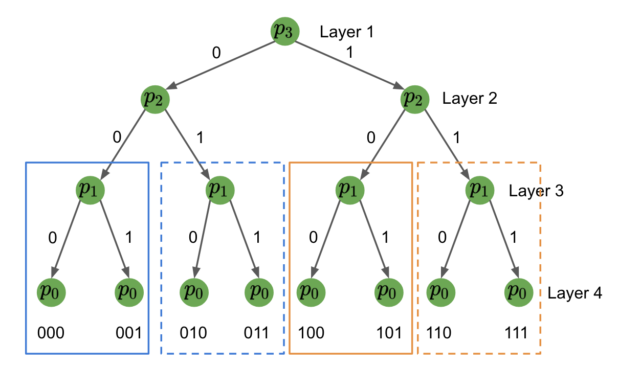
Figure 1: An $8$-cluster Binary Tree SBM. Rectangles correspond to mega-communities.

A recent work by Li et al. (2018a) established a framework to study divisive hierarchical clustering. They proposed the Binary Tree SBM (BTSBM) as the basis for analysis. A BTSBM is an SBM, described in Section 5.1, with $K=2^{d}$ clusters, embedded into the leaf nodes of a full binary tree with $d+1$ layers. The $\ell$-th layer is equipped with a parameter $p_{d-\ell+1}$ and each cluster is encoded as a length-$d$ binary string. We illustrate it in Figure 1 with $d=3$. The connection probability matrix $B$ is then decided as follows: for any two clusters $c$ and $c^{\prime}$, let $x_{d}\ldots x_{1}$ and $x_{d}^{\prime}\ldots x_{1}^{\prime}$ be their binary representation, then

$$B_{c,c^{\prime}}=p_{\scriptscriptstyle{D(c,c^{\prime})}},\quad\mbox{where }D(c,c^{\prime})=\max\{i:x_{i}\not=x_{i}^{\prime}\}I(c\not=c^{\prime}).$$

For instance, for the BTSBM in Figure 1,

$$B=\left[\begin{array}[]{cc|cc|cccc}p_{0}&p_{1}&p_{2}&p_{2}&p_{3}&p_{3}&p_{3}&p_{3}\\ p_{1}&p_{0}&p_{2}&p_{2}&p_{3}&p_{3}&p_{3}&p_{3}\\ \hline\cr p_{2}&p_{2}&p_{0}&p_{1}&p_{3}&p_{3}&p_{3}&p_{3}\\ p_{2}&p_{2}&p_{1}&p_{0}&p_{3}&p_{3}&p_{3}&p_{3}\\ \hline\cr p_{3}&p_{3}&p_{3}&p_{3}&p_{0}&p_{1}&p_{2}&p_{2}\\ p_{3}&p_{3}&p_{3}&p_{3}&p_{1}&p_{0}&p_{2}&p_{2}\\ p_{3}&p_{3}&p_{3}&p_{3}&p_{2}&p_{2}&p_{0}&p_{1}\\ p_{3}&p_{3}&p_{3}&p_{3}&p_{2}&p_{2}&p_{1}&p_{0}\end{array}\right].$$ (63)

Assuming equal block sizes for all communities, Li et al. (2018a) analyzed the HCD-Sign algorithm, which splits the network nto two mega-communities according to the sign of the second eigenvector of the adjacency matrix, under both assortative BTSBM ($p_{0}>p_{1}>\ldots>p_{d}$) and dis-assortative BTSBM ($p_{0}<p_{1}<\ldots<p_{d}$). They provided explicit conditions under which all mega-communities in the first $\ell$ layers can be exactly recovered for any $\ell\leq d$. Unlike the $K$-way spectral clustering, described in Section 5.1, which requires knowing $K$ exactly, HCD-Sign can be completely agnostic to $K$ while only requires a “consistent” stopping rule, such as the one based on non-backtracking operator (Le and Levina, 2015).

The proof relies on the nice eigen-structure of BTSBM as stated below.

Proposition 6.1.

[Theorem 5 of Li et al. (2018a)] Under either assortative or dis-assorative BTSBM,

1. the first and the second largest eigenvalue (in absolute value) of $A^{*}$ are both unique, given by

   $$\lambda_{1}^{*}=(m-1)p_{0}+m\sum_{i=1}^{d-1}2^{i-1}p_{i}+m2^{d-1}p_{d},\quad\lambda_{2}^{*}=(m-1)p_{0}+m\sum_{i=1}^{d-1}2^{i-1}p_{i}-m2^{d-1}p_{d};$$

2. the eigen-gap $\Delta^{*}$ between $\lambda_{2}^{*}$ and others is

   $$\Delta^{*}=\left\{\begin{array}[]{ll}n\min\{p_{d},|p_{d-1}-p_{d}|/2\}&\mbox{(for assortative BTSBM)}\\ n|p_{d-1}-p_{d}|/2&\mbox{(for dis-assortative BTSBM)}\end{array}\right.;$$

3. the eigenvector corresponding to $\lambda_{2}^{*}$ is

   $$u_{2}=\frac{1}{\sqrt{n}}\begin{bmatrix}\textbf{1}_{n/2}\\ -\textbf{1}_{n/2}\end{bmatrix};$$

4. $\mathrm{rank}(A^{*})=K$. $A^{*}$ is psd under assortative BTSBM, but not psd under dis-assortative BTSBM.

Proposition 6.1 implies that the second eigenvector of $A^{*}$ perfectly identifies the binary split. They proceed by showing that $\|u_{2}-u_{2}^{*}\|_{\infty}<\!\!<1/\sqrt{n}$ thereby proving the exact recovery for each split. The technique underlying their analysis is derived by Eldridge et al. (2017).

Although BTSBM is still restrictive, it is much more general than the typical four-parameter model described in Section 5.3. More importantly, BTSBM captures the multi-scale nature of real-world networks: the clusters are not treated as “exchangeable” but encoding different granularity of similarity. Furthermore, divisive hierarchical clustering algorithms are able to achieve partial recovery, i.e. recovering mega-communities up to layer $\ell+1$ without recovering the communities at the finest level, imply that the stable structure (i.e. mega-communities) may be recovered even if the finest communities cannot, depending on how similar different clusters are.

With the new $\ell_{2\rightarrow\infty}$ perturbation bounds in this paper, we can refine Li et al. (2018a)’s results and obtain a more accurate characterization of the partial exact recovery phenomenon. We start from a generic sufficient condition for recovering one split and then apply it to analyze the case with fixed $K$. The case with growing $K$ can be analyzed similarly but we leave it to interested readers for the sake of length.

6.2 A generic sufficient condition for recovering one split

The exact recovery for the first split is achieved by HCD-Sign iff there exists $s\in\{-1,+1\}$ such that

$$\mathrm{sign}(u_{2i}^{*})=\mathrm{sign}(u_{2i})s,\quad\forall i\in[n].$$ (64)

As observed by Abbe et al. (2017) as well as our theory, $u_{2}$ is closer to $Au_{2}^{*}/\lambda_{2}^{*}$ than to $u_{2}^{*}$. The following lemma provides a sufficient condition for 64 based on $Au_{2}^{*}/\lambda_{2}^{*}$.

Lemma 6.2.

64 holds if there exists $s\in\{-1,+1\}$ such that for all $i\in[n]$,

$$\mathrm{sign}(u_{2i}^{*})=\mathrm{sign}(A_{i}^{T}(\sqrt{n}u_{2}^{*}))s,$$ (65)

and

$$|A_{i}^{T}(\sqrt{n}u_{2}^{*})|>\left(\sqrt{n}\bigg{\|}u_{2}-\frac{Au_{2}^{*}}{\lambda_{2}^{*}}\bigg{\|}_{\infty}\right)|\lambda_{2}^{*}|.$$ (66)

Proof.

We only prove the assortative case and the proof for the dissortative case is similar. Assume $s=1$ without loss of generality. The condition66 can be rewritten as

$$\bigg{|}\frac{A_{i}^{T}u_{2}^{*}}{\lambda_{2}^{*}}\bigg{|}>\bigg{\|}u_{2}-\frac{Au_{2}^{*}}{\lambda_{2}^{*}}\bigg{\|}_{\infty}\geq\bigg{|}u_{2i}-\frac{A_{i}^{T}u_{2}^{*}}{\lambda_{2}^{*}}\bigg{|}.$$

By Proposition 6.1, $\lambda_{2}^{*}>0$ and

$$\mathrm{sign}(u_{2i})=\mathrm{sign}\left(\frac{A_{i}^{T}u_{2}^{*}}{\lambda_{2}^{*}}\right)=\mathrm{sign}(A_{i}^{T}(\sqrt{n}u_{2}^{*})).$$

Together with condition 65, we complete the proof. ∎

By Proposition 6.1,

$$A_{i}^{T}(\sqrt{n}u_{2}^{*})=\sum_{j=1}^{n/2}A_{ij}-\sum_{j=n/2+1}^{n}A_{ij}.$$ (67)

Let

$$Z_{i}=(-1)^{I(i>n/2)}A_{i}^{T}(\sqrt{n}u_{2}^{*})$$ (68)

Under BTSBM, it is not hard to see that $Z_{1},\ldots,Z_{n}$ are i.i.d.. Note that $\mathrm{sign}(u_{2i}^{*})=(-1)^{I(i>n/2)}$. By Lemma 6.2, 65 and 66 are both satisfied if

$$\min_{i\in[n]}Z_{i}>\left(\sqrt{n}\bigg{\|}u_{2}-\frac{Au_{2}^{*}}{\lambda_{2}^{*}}\bigg{\|}_{\infty}\right)|\lambda_{2}^{*}|\quad\mbox{or}\quad\max_{i\in[n]}Z_{i}<-\left(\sqrt{n}\bigg{\|}u_{2}-\frac{Au_{2}^{*}}{\lambda_{2}^{*}}\bigg{\|}_{\infty}\right)|\lambda_{2}^{*}|.$$ (69)

It is left to show the above event occurs with high probability.

The following lemma provides a tail probability estimate for $Z_{i}$. The proof is relegated to Appendix D.3.

Lemma 6.3.

1. In the assortative case, for any $t>0$,

   $$\log\mathbb{P}(Z_{i}\leq t)\leq\frac{t}{2}\log\left(\frac{\lambda_{1}^{*}+\lambda_{2}^{*}}{\lambda_{1}^{*}-\lambda_{2}^{*}}\right)-\frac{1}{2}\left(\sqrt{\lambda_{1}^{*}+\lambda_{2}^{*}}-\sqrt{\lambda_{1}^{*}-\lambda_{2}^{*}}\right)^{2}.$$

2. In the dis-assortative case, for any $t>0$,

   $$\log\mathbb{P}(Z_{i}\geq-t)\leq\frac{t}{2}\log\left(\frac{\lambda_{1}^{*}-\lambda_{2}^{*}}{\lambda_{1}^{*}+\lambda_{2}^{*}}\right)-\frac{1}{2}\left(\sqrt{\lambda_{1}^{*}+\lambda_{2}^{*}}-\sqrt{\lambda_{1}^{*}-\lambda_{2}^{*}}\right)^{2}.$$

Combined with the high probability upper bound for $\|u_{2}-Au_{2}^{*}/\lambda_{2}^{*}\|_{\infty}$ obtained by Theorem 3.4, we can derive the following result for recovering the first split exactly. The proof is straightforward so we relegate it into Appendix D.3.

Theorem 6.4.

Consider a BTSBM that is either assortative or dis-assortative. Let $\Delta^{*}$ be defined as in Proposition 6.1 and $p^{*}=\max\{p_{0},p_{d}\}$. Suppose there exists $\alpha>0$ and $q>0$ such that

$$\Delta^{*}>(q+1)C\left(\sqrt{\lambda_{1}^{*}}+\frac{\log n}{\alpha\log\log n}\right),$$ (70)

where $C$ is the universal constant in 19. Fix any $\delta\geq n^{-q}$. Then the first split can be recovered with probability $1-2\delta$ if

$$\frac{1}{2}\left(\sqrt{\lambda_{1}^{*}+\lambda_{2}^{*}}-\sqrt{\lambda_{1}^{*}-\lambda_{2}^{*}}\right)^{2}-\log n-C^{\prime}\frac{\lambda_{2}^{*}}{\Delta^{*}}\bigg{|}\log\left(\frac{\lambda_{1}^{*}+\lambda_{2}^{*}}{\lambda_{1}^{*}-\lambda_{2}^{*}}\right)\bigg{|}(\xi_{n1}+\xi_{n2})\geq\log\left(\frac{1}{\delta}\right),$$ (71)

where $C^{\prime}$ is a universal constant and

$$\xi_{n1}=\left(\sqrt{\lambda_{1}^{*}}+\frac{\log n}{\alpha\log\log n}\right)\left(1+\frac{\log n}{|\lambda_{2}^{*}|}\right)+\frac{\sqrt{(\log n)np^{*}}}{|\lambda_{2}^{*}|}\frac{\log n+\sqrt{\lambda_{1}^{*}(\log n)^{\alpha}}}{\alpha\log\log n},$$

and

$$\xi_{n2}=\left\{\begin{array}[]{ll}\min\left\{\sqrt{np^{*}},\sqrt{\lambda_{2}^{*}K}\right\}&\mbox{(assortative)}\\ \min\left\{\sqrt{\lambda_{1}^{*}np^{*}/|\lambda_{2}^{*}|},\sqrt{\lambda_{2}^{*}K}\right\}&\mbox{(dis-assortative)}\\ \end{array}\right..$$

6.3 Exact recovery of mega-communities for BTSBMs

Consider the setting where $K$ is fixed and

$$p_{j}=\rho_{n}a_{j},$$

for a set of constants $(a_{0},\ldots,a_{d})$. Li et al. (2018a) proves the exact recovery in the regime $n\rho_{n}\succeq(\log n)^{2+\epsilon}$. On the other hand, if $K$ is known, the information theoretic lower bound for recovering all communities (not including mega-communities) is $\rho_{n}=\log n/n$ (e.g. Abbe and Sandon, 2015). The extra logarithmic factors in Li et al. (2018a) is simply an artifact of using the non-tight $\ell_{\infty}$ perturbation bound by Eldridge et al. (2017). With Theorem 6.4 derived from our $\ell_{\infty}$ perturbation theory, we can prove the exact recovery in the regime $\rho_{n}=\log n/n$ and provide precise condition on the constants $(a_{0},\ldots,a_{d})$.

Theorem 6.5.

Assume that $\rho_{n}=\log n/n$ and either $a_{0}>a_{1}>\ldots>a_{d}>0$ (assortative) or $0<a_{0}<a_{1}<\ldots<a_{d}$ (dis-assortative). Fix any $\ell\in[d]$. If further

$$|\sqrt{\bar{a}_{r}}-\sqrt{a_{r}}|>\sqrt{2^{d-r+1}},\quad r=d,d-1,\ldots,d-\ell+1,$$ (72)

where

$$\bar{a}_{r}=\frac{a_{0}+\sum_{j=1}^{r-1}2^{j-1}a_{j}}{2^{r-1}},$$ (73)

then all mega-communities up to layer $\ell+1$ can be exactly recovered with probability $1-o(1)$ as $n$ tends to infinity.

Remark 6.1.

The quantity $\bar{a}_{r}$ is essentially the average conncetion probability in each mega-community at $(d-r+2)$-th layer.

The condition 72 has an interesting implication. Take $\ell=d$, it is equivalent to

$$|\sqrt{\bar{a}_{d}}-\sqrt{a_{d}}|>\sqrt{2}.$$

Further take $d=3$ for illustration and recall 63. Consider the following hypothetical SBM with connection probability matrix

$$B^{\prime}=\rho_{n}\left[\begin{array}[]{cccc|cccc}\bar{a}_{3}&\bar{a}_{3}&\bar{a}_{3}&\bar{a}_{3}&a_{3}&a_{3}&a_{3}&a_{3}\\ \bar{a}_{3}&\bar{a}_{3}&\bar{a}_{3}&\bar{a}_{3}&a_{3}&a_{3}&a_{3}&a_{3}\\ \bar{a}_{3}&\bar{a}_{3}&\bar{a}_{3}&\bar{a}_{3}&a_{3}&a_{3}&a_{3}&a_{3}\\ \bar{a}_{3}&\bar{a}_{3}&\bar{a}_{3}&\bar{a}_{3}&a_{3}&a_{3}&a_{3}&a_{3}\\ \hline\cr a_{3}&a_{3}&a_{3}&a_{3}&\bar{a}_{3}&\bar{a}_{3}&\bar{a}_{3}&\bar{a}_{3}\\ a_{3}&a_{3}&a_{3}&a_{3}&\bar{a}_{3}&\bar{a}_{3}&\bar{a}_{3}&\bar{a}_{3}\\ a_{3}&a_{3}&a_{3}&a_{3}&\bar{a}_{3}&\bar{a}_{3}&\bar{a}_{3}&\bar{a}_{3}\\ a_{3}&a_{3}&a_{3}&a_{3}&\bar{a}_{3}&\bar{a}_{3}&\bar{a}_{3}&\bar{a}_{3}\end{array}\right].$$ (74)

This is essentially a $2$-block SBM with parameter $\bar{a}_{3}\log n/n$ and $a_{3}\log n/n$ where $\bar{a}_{3}$ is the average probability in the mega-community. It is well-known that 74 can be exactly recovered if and only if

$$|\sqrt{\bar{a}_{3}}-\sqrt{a_{3}}|>\sqrt{2}.$$

In other words, recovering the first split of the BTSBM with connection probability matrix 63 is indistinguishable from recovering the blocks if the induced $2$-block model, which replaces the connection probabilities by the within-mega-community average. This is an unexpected robustness result for mis-specified SBM models.

On the other hand, as mentioned earlier, we want to investigate the possibility that the finest communites cannot be recovered but higher-level mega-communities can. To investigate this, we first derive the necessary condition for the exact recovery of $K$ communities in the leaf nodes. This is a simple consequence of the existing results on general SBMs (e.g. Abbe and Sandon, 2015).

Lemma 6.6.

No algorithm can recovery all of $K$ communities in the leaf nodes of a BTSBM, that is either assortative or dis-assortative, with high probability if

$$|\sqrt{a_{0}}-\sqrt{a_{1}}|<\sqrt{K}.$$ (75)

Note that $\bar{a}_{1}=a_{0}$. The necessary condition 75 is essentially the negation of 72 with $\ell=d$ and $r=1$. If $|\sqrt{a_{0}}-\sqrt{a_{1}}|<\sqrt{K}$, Lemma 6.6 implies that the finest communities cannot be recovered exactly by any algorithm, including HCD algorithms. However, if 72 holds for $\ell=d-1$, we may recover all mega-communities up to the second last layers. This is true, for instance, if $a_{0}\approx a_{1}$ and

$$|\sqrt{\bar{a}_{r}^{\prime}}-\sqrt{a_{r}}|>\sqrt{2^{d-r+1}},\quad r=d,d-1,\ldots,2,$$

where

$$\bar{a}_{r}^{\prime}=\frac{a_{1}+\sum_{j=1}^{r-1}2^{j-1}a_{j}}{2^{r-1}}.$$

Therefore, Theorem 6.5 provides a precise characterization of the partial exact recovery phenomenon.

7 Extensions

7.1 Random matrices with other dependency structure

In Section 3.2 we discuss the unnormalized Laplacian as an example of random matrices with dependent entries. From assumption A1, it is not hard to see that our generic bounds allow much more flexible dependency structure. As shown in part (b) of Proposition 2.1, A1 is satisfied if the rows are $m$-dependent. If we can further derive bounds for $\|E\|_{\mathrm{op}}$ and $E_{k}^{T}W$ as in A2 and A3, Theorem 2.3 would yield an $\ell_{2\rightarrow\infty}$ perturbation bound.

Concentration inequalities for both quantities have been investigated for various dependency structures. We consider a slightly artificial one, motivated by Paulin (2012), just to illustrate the possibility to handle complex dependency structure. In particular, we assume that $A_{ij}$’s can be partitioned into $M$ subsets such that the entries within the same block are independent while the blocks can be arbitrarily dependent. In this case, $E$ can be decomposed as the sum of $M$ matrices $\{E^{(\ell)}:\ell\in[M]\}$ where $E^{(\ell)}_{ij}=E_{ij}$ if $(i,j)$ belongs to the $\ell$-th block and $E^{(\ell)}_{ij}=0$ otherwise. By Lemma 3.2 and a union bound,

$$\lambda_{-}(\delta),E_{+}(\delta),\bar{E}_{+}(\delta),E_{\infty}(\delta)\preceq E_{2}(\delta)\preceq M\left(\sqrt{n\bar{p}^{*}}+\sqrt{\log(nM/\delta)}\right).$$

On the other hand, we apply the same decomposition on $E_{k}^{T}W$ and Lemma 3.1 implies that

$$b_{\infty}(\delta)\preceq\frac{MR(\delta/M)}{\alpha\log R(\delta/M)},\quad b_{2}(\delta)\preceq\frac{M\sqrt{p^{*}}R(\delta/M)^{(1+\alpha)/2}}{\alpha\log R(\delta/M)}.$$

Given these bounds, it is a simple exercise to derive the condition on $\Delta^{*}$ through A4 as well as the $\ell_{2\rightarrow\infty}$ bound for $d_{2\rightarrow\infty}(U,AU^{*}(\Lambda^{*})^{-1})$ and $d_{2\rightarrow\infty}(U,U^{*})$ by Theorem 2.3 and Theorem 2.4. It is also straightforward to derive the bounds for the unnormalized Laplacian using the results in Section 2.3.

The above case is by no means the end of the story. More complicated dependency structures can be handled similarly using more delicate bounds (e.g. Paulin, 2012). The punchline is that our theory reduces the less tractable $\ell_{2\rightarrow\infty}$ perturbation bound to the more tractable concentration bounds on $E$.

7.2 Non-binary random matrices

Our result can also be easily extended to non-binary random matrices. For instance, for Gaussian random matrices with $A_{ij}\stackrel{{\scriptstyle\mathrm{indep.}}}{{\sim}}N(\mu_{ij},\sigma_{ij}^{2})$, Corollary 3.9 of Bandeira and Van Handel (2016) implies that

$$E_{2}(\delta)\preceq\bar{\sigma}^{*}\sqrt{n}+\sigma^{*}\sqrt{\log\left(\frac{n}{\delta}\right)},\quad\mbox{where }\bar{\sigma}^{*}=\max_{i}\sqrt{\frac{1}{n}\sum_{j=1}^{n}\sigma_{ij}^{2}},\quad\sigma^{*}=\max_{i}\sigma_{ij}.$$

This establishes the bounds for quantities in assumption A2. By Propostion 2.1,

$$L_{1}(\delta)\preceq\|A^{*}\|_{2\rightarrow\infty}+E_{2}(\delta),\quad L_{2}(\delta)\preceq 1,\quad L_{3}(\delta)\preceq(\|A^{*}\|_{2\rightarrow\infty}+E_{2}(\delta))/\lambda_{\min}^{*}.$$

On the other hand, for any $W\in\mathbb{R}^{n\times r^{\prime}}$ with $r^{\prime}\leq r$, $E_{k}^{T}W\sim N(0,W^{T}D_{k}W)$ where $D_{k}=\mathrm{diag}(\sigma_{kj}^{2})_{j=1}^{n}$. Thus, $E_{k}^{T}W\stackrel{{\scriptstyle d}}{{=}}(W^{T}D_{k}W)^{1/2}X$ where $X\sim N(0,I_{r^{\prime}})$. Since the mapping $f:x\mapsto\|((W^{T}D_{k}W)^{1/2})x\|_{2}$ is $\|W^{T}D_{k}W\|_{\mathrm{op}}$-Lipschitz and $\|W^{T}D_{k}W\|_{\mathrm{op}}\leq\sigma^{*}\|W\|_{\mathrm{op}}$, by Gaussian concentration inequality,

$$\mathbb{P}\left(\|E_{k}^{T}W\|_{2}\geq\mathbb{E}\|E_{k}^{T}W\|_{2}+t\right)\leq\exp\left\{-\frac{t^{2}}{\sigma^{*2}\|W\|_{\mathrm{op}}^{2}}\right\}.$$

Taking $t=\sigma^{*}\|W\|_{\mathrm{op}}\sqrt{\log(n/\delta)}$, we know that

$$\|E_{k}^{T}W\|_{2} \leq\mathbb{E}\|E_{k}^{T}W\|_{2}+t\leq\sqrt{\mathbb{E}\|E_{k}^{T}W\|_{2}^{2}}+t\leq\sqrt{\operatorname*{tr}(W^{T}D_{k}W)}+t$$

$$\leq\|W\|_{\mathrm{op}}\sigma^{*}\left(\sqrt{r}+\sqrt{\log(n/\delta)}\right)\preceq\sigma^{*}R(\delta)\|W\|_{\mathrm{op}}.$$

As a result, we have $b_{\infty}(\delta)=0$ and $b_{2}(\delta)\preceq\sigma^{*}R(\delta)$ in Assumption A3. As commented in Remark 2.2,

$$\|EU^{*}\|_{2\rightarrow\infty}\preceq\sigma^{*}R(\delta).$$

Putting pieces together, we can derive the $\ell_{2\rightarrow\infty}$ bound in this case by Theorem 2.3 and Theorem 2.4.

Following the same strategy, we can extend the results to other entry distributions. The bound for $\|E\|_{\mathrm{op}}$ can be found in Bandeira and Van Handel (2016); Latała et al. (2018); Rebrova (201) for sub-gaussian, sub-exponential, heavy-tailed, symmetric random variables. The row-wise concentration inequality can be obtained from standard moment generating function arguments (e.g. Vershynin, 2010).

7.3 Asymmetric random matrices

Our perturbation bound can be extended to asymmetric and rectangular matrices using the Hermitian dilation trick (e.g. Paulsen, 2002). Given a rectangular matrix $A\in\mathbb{R}^{m\times n}$ with $m\geq n$, the Hermitian dilation of $A$ is defined as

$$\tilde{A}=\begin{bmatrix}0&A\\ A^{T}&0\end{bmatrix},$$

Let $\bar{U}\bar{\Sigma}\bar{V}^{T}$ be the singular value decomposition (SVD) of $A$ where $\bar{U}\in\mathbb{R}^{m\times n},\bar{V}\in\mathbb{R}^{n\times n}$ are two orthogonal matrices and $\bar{\Sigma}\in\mathbb{R}^{n\times n}$ is a diagonal matrix. Then $\tilde{U}\tilde{\Sigma}\tilde{U}^{T}$ is the SVD of $\tilde{A}$ where

$$\tilde{U}=\frac{1}{\sqrt{2}}\begin{bmatrix}\bar{U}&\bar{U}\\ \bar{V}&-\bar{V}\end{bmatrix},\quad\tilde{\Sigma}=\begin{bmatrix}\bar{\Sigma}&0\\ 0&-\bar{\Sigma}\\ \end{bmatrix}.$$

Given a pair of asymmetric matrices $A,A^{*}\in\mathbb{R}^{m\times n}$, their left singular spaces $U,U^{*}$ and corresponding right singular spaces $V,V^{*}$, our bound can be applied to their Hermitian dilation to yield a bound for

$$d_{2\rightarrow\infty}\left(\begin{bmatrix}U\\ V\end{bmatrix},\begin{bmatrix}U^{*}\\ V^{*}\end{bmatrix}\right).$$

This provides an upper bound for both $d_{2\rightarrow\infty}(U,U^{*})$ and $d_{2\rightarrow\infty}(V,V^{*})$.

7.4 Perturbation in other metrics

Given an $\ell_{2\rightarrow\infty}$ bound, we can derive the perturbation bound in other metrics. One example is the $\ell_{2\rightarrow\infty}$ bound for projection matrices, namely $\|UU^{T}-U^{*}(U^{*})^{T}\|_{2\rightarrow\infty}$, which is studied in Mao et al. (2017). Note that for any $O\in\mathcal{O}^{r}$,

$$UU^{T}-U^{*}(U^{*})^{T}=U\mathcal{O}(U\mathcal{O})^{T}-U^{*}(U^{*})^{T}=(U\mathcal{O}-U^{*})(U\mathcal{O})^{T}+U^{*}(U\mathcal{O}-U^{*})^{T}.$$

Then

$$\|(U\mathcal{O}-U^{*})(U\mathcal{O})^{T}\|_{2\rightarrow\infty}\leq\|U\mathcal{O}-U^{*}\|_{2\rightarrow\infty}\|U\mathcal{O}\|_{\mathrm{op}}=\|U\mathcal{O}-U^{*}\|_{2\rightarrow\infty},$$

and

$$\|U^{*}(U\mathcal{O}-U^{*})^{T}\|_{2\rightarrow\infty}\leq\|U^{*}\|_{2\rightarrow\infty}\|U\mathcal{O}-U^{*}\|_{\mathrm{op}}\leq\sqrt{n}\|U^{*}\|_{2\rightarrow\infty}\|U\mathcal{O}-U^{*}\|_{2\rightarrow\infty}.$$

Taking $O$ as the orthogonal matrix that minimizes $\|U\mathcal{O}-U^{*}\|_{2\rightarrow\infty}$, we conclude that

$$\|UU^{T}-U^{*}(U^{*})^{T}\|_{2\rightarrow\infty}\leq(\sqrt{n}\|U^{*}\|_{2\rightarrow\infty}+1)\|U\mathcal{O}-U^{*}\|_{2\rightarrow\infty}\preceq\sqrt{n}\|U^{*}\|_{2\rightarrow\infty}\|U\mathcal{O}-U^{*}\|_{2\rightarrow\infty}.$$

Another example is the entrywise bound for $UU^{T}-U^{*}(U^{*})^{T}$. For any $O\in\mathcal{O}^{r}$, we have

$$UU^{T}-U^{*}(U^{*})^{T}=(U\mathcal{O}-U^{*})(U\mathcal{O}-U^{*})^{T}+U^{*}(U\mathcal{O}-U^{*})^{T}+(U\mathcal{O}-U^{*})(U^{*})^{T}.$$

Taking $O\in\mathcal{O}^{r}$ that minimizes $\|U\mathcal{O}-U^{*}\|_{2\rightarrow\infty}$ and using the fact that $\|AB\|_{\max}\leq\|A\|_{2\rightarrow\infty}\|B\|_{2\rightarrow\infty}$, we have

$$\|UU^{T}-U^{*}(U^{*})^{T}\|_{\max}\preceq d_{2\rightarrow\infty}(U,U^{*})^{2}+\|U^{*}\|_{2\rightarrow\infty}d_{2\rightarrow\infty}(U,U^{*}).$$

Finally, we can derive an entry-wise bound for $U\Lambda U^{T}-U^{*}\Lambda^{*}(U^{*})^{T}$, which is of interest if the goal is to recover the low-rank component. Similar to the derivation for projection matrices, by Weyl’s inequality,

$$\|U\Lambda U^{T}-U^{*}\Lambda^{*}(U^{*})^{T}\|_{\max} \preceq d_{2\rightarrow\infty}(U,U^{*})\|U^{*}\|_{2\rightarrow\infty}\lambda_{\max}^{*}+\|U^{*}\|_{2\rightarrow\infty}^{2}\|E\|_{\mathrm{op}}$$

$$+d_{2\rightarrow\infty}(U,U^{*})^{2}\lambda_{\max}^{*}+d_{2\rightarrow\infty}(U,U^{*})^{2}\|E\|_{\mathrm{op}}.$$

Appendix A Proof of Theorem 2.3

The proof is very involved, so we split the proof into six steps.

A.1 Notation

Let $\mathcal{O}^{r}$ denote the space of all $r\times r$ orthogonal matrices and $\textbf{1}_{n}$ denote a $n$-dimensional vector with all entries $1$. For any vector $x$, let $\|x\|_{p}$ denotes its $p$-norm. For any matrix $M$, denote by $M_{k}^{T}$ the $m$-th row of $M$, by $\|M\|_{\mathrm{op}}$ its operator norm and by $\|M\|_{\mathrm{F}}$ its Frobenius norm. Moreover, for any $p,q\in[1,\infty]$, let

$$\|M\|_{p\rightarrow q}=\sup_{\omega:\|\omega\|_{p}=1}\|M\omega\|_{q}.$$

In particular,

$$\|M\|_{2\rightarrow\infty}=\max_{k}\|M_{k}\|_{2}.$$

Suppose $U\Sigma V^{T}$ is the singular value decomposition of $M$. When $M$ is a square matrix, we define the matrix sign as

$$\mathrm{sign}(M)=UV^{T}.$$

By definition, $\mathrm{sign}(M)$ is orthogonal. When $n=1$, $M$ is a scalar and $\mathrm{sign}(M)$ reduces to the classical sign of scalars. Further we denote by $\lambda_{\max}(M)$ (resp. $\lambda_{\min}(M)$) the largest (resp. the smallest) eigenvalue of $M$ in absolute values and by $\kappa(M)$ the condition number $\lambda_{\max}(M)/\lambda_{\min}(M)$. We say a square matrix $M$ positive semi-definite (psd) if all eigenvalues of $M$ are non-negative. In particular, we write $\lambda_{\max}(\Lambda^{*})$ (resp. $\lambda_{\min}(\Lambda^{*})$) as $\lambda_{\min}^{*}$ (resp. $\lambda_{\max}^{*}$) and $\kappa(\Lambda^{*})$ as $\kappa^{*}$ for short.

For any matrices $U,Z\in\mathbb{R}^{n\times r}$ with orthonormal columns, let $\Theta$ denote the principal angle matrix between the two subspaces spanned by $U$ and $Z$, such that $U^{T}Z$ has the singular value decomposition $U^{T}Z=\bar{U}(\cos\Theta)\bar{V}^{T}$ where $\Theta=\mathrm{diag}(\theta_{1},\ldots,\theta_{r})$ with $\theta_{j}\in[0,\frac{\pi}{2}]$.

For any Hermitian matrices $B_{1},B_{2}\in\mathbb{R}^{n\times n}$, let $\lambda_{1}(B_{j})\geq\lambda_{2}(B_{j})\geq\ldots\geq\lambda_{n}(B_{j})$ be the eigenvalues of $B_{j}(j=1,2)$. Let

$$\mathrm{sep}_{s+1,s+r}(B_{1},B_{2})=\min\{|\lambda_{i}(B_{1})-\lambda_{j}(B_{2})|:i\not\in\{s+1,\ldots,s+r\},j\in\{s+1,\ldots,s+r\}\}.$$

Note that $\mathrm{sep}_{s+1,s+r}$ is not symmetric in the sense that $\mathrm{sep}_{s+1,s+r}(B_{1},B_{2})\not=\mathrm{sep}_{s+1,s+r}(B_{2},B_{1})$. When $B_{1}=B_{2}=B$, we write it as $\mathrm{sep}_{s+1,s+r}(B)$ for short.

A.2 Preparation: preliminary properties

When $r=1$, $U$ and $U^{*}$ are vectors and it is straightforward to show that

$$d_{2\rightarrow\infty}(U,U^{*})=\|U\mathrm{sign}(U^{T}U^{*})-U^{*}\|_{2\rightarrow\infty}.$$

This motivates us to consider an upper bound of $d_{2\rightarrow\infty}(U,U^{*})$ as

$$d_{2\rightarrow\infty}(U,U^{*})\leq\|U\mathrm{sign}(H)-U^{*}\|_{2\rightarrow\infty},$$ (76)

where

$$H=U^{T}U^{*}.$$ (77)

Similarly for distance between $U$ and $AU^{*}(\Lambda^{*})^{-1}$, we consider the upper bound

$$d_{2\rightarrow\infty}(U,AU^{*}(\Lambda^{*})^{-1})\leq\|U\mathrm{sign}(H)-AU^{*}(\Lambda^{*})^{-1}\|_{2\rightarrow\infty}.$$ (78)

This was also considered in Abbe et al. [2017]. Our goal is to derive upper bounds for 78 and 76.

Finally, let $A^{(1)},\ldots,A^{(n)}$ be $n$ auxiliary matrices that satisfy the following condition, as the deterministic analogue of assumption A1 with $S=[r]$.

1. There exists $L_{1},L_{2},L_{3}$ such that for all $k$,

   $$\|A^{(k)}-A\|_{\mathrm{op}}\leq L_{1},\quad\frac{\|(A^{(k)}-A)U\|_{\mathrm{op}}}{\lambda_{\min}^{*}}\leq\left(\kappa^{*}L_{2}+L_{3}\right)\|U\|_{2\rightarrow\infty}.$$

Similarly we define $\Lambda^{(k)}$ as the diagonal matrix given by the $(s+1)$-th to the $(s+r)$-th largest eigenvalues and $U^{(k)}\in\mathbb{R}^{n\times r}$ as a matrix of eigenvectors corresponding to $\Lambda^{(k)}$ i.e.

$$A^{(k)}U^{(k)}=U^{(k)}\Lambda^{(k)}.$$

Further let

$$H^{(k)}=(U^{(k)})^{T}U^{*}.$$

The following proposition provides a simple yet important property of eigen-separation.

Proposition A.1.

For any Hermitian matrices $B_{1},B_{2}\in\mathbb{R}^{n\times n}$,

$$\mathrm{sep}_{s+1,s+r}(B_{1},B_{2})\geq\max\{\mathrm{sep}_{s+1,s+r}(B_{1}),\mathrm{sep}_{s+1,s+r}(B_{2})\}-\max_{i\in[s+1,s+r]}|\lambda_{i}(B_{1})-\lambda_{i}(B_{2})|.$$

Proof.

For any $i,j$,

$$|\lambda_{i}(B_{1})-\lambda_{j}(B_{2})| \geq|\lambda_{i}(B_{2})-\lambda_{j}(B_{2})|-|\lambda_{i}(B_{1})-\lambda_{i}(B_{2})|.$$

The proof is completed by considering all pairs of $i$ and $j$. ∎

Based on Proposition A.1, we can derive the eigen-separation among $A$, $A^{*}$ and $A^{(k)}$.

Lemma A.2.

Let $E$ be defined as in 1. Under condition C0,

$$\mathrm{sep}_{s+1,s+r}(A,A^{*})\geq\mathrm{sep}_{s+1,s+r}(A^{*})-\|\Lambda-\Lambda^{*}\|_{\max},$$

and for any $k$,

$$\mathrm{sep}_{s+1,s+r}(A^{(k)},A)\geq\mathrm{sep}_{s+1,s+r}(A^{*})-L_{1}-2\|\Lambda-\Lambda^{*}\|_{\max}.$$

Proof.

The first part is a direct result of Proposition A.1. By definition,

$$\|A^{(k)}-A\|_{\mathrm{op}}\leq L_{1}.$$

The second part is then proved by noting that

$$\mathrm{sep}_{s+1,s+r}(A^{(k)},A)\geq\mathrm{sep}_{s+1,s+r}(A)-\|A^{(k)}-A\|_{\mathrm{op}}$$

where the last inequality uses Weyl’s inequality and

$$\mathrm{sep}_{s+1,s+r}(A)\geq\mathrm{sep}_{s+1,s+r}(A,A^{*})-\|\Lambda-\Lambda^{*}\|_{\max}\geq\mathrm{sep}_{s+1,s+r}(A^{*})-2\|\Lambda-\Lambda^{*}\|_{\max}.$$

∎

Recall the definition of $\Delta^{*}$ in 4 and let

$$\Gamma=\frac{\Delta^{*}-L_{1}}{2}.$$ (79)

Note that the first term of $\Gamma$ is essentially the half eigen-gap if $0$ is an eigenvalue but not in $\Lambda^{*}$. Under assumption A4, $\Gamma$ has the same order as $\Delta^{*}$. Throughout the rest of this section, we assume the following condition:

1. $\|\Lambda-\Lambda^{*}\|_{\max}\leq\Gamma/2$ where $E$ is defined in 1 and $\Gamma$ is defined in 79.

Corollary A.3.

Under condition C0 and C1,

$$\min\{\mathrm{sep}_{s+1,s+r}(A,A^{*}),\mathrm{sep}_{s+1,s+r}(A^{(k)},A)\}\geq\Gamma.$$

The above results on eigen-gaps allow us to apply Davis-Kahan Theorem [Davis and Kahan, 1970] to bound the discrepancy between the eigenspaces of $A$ and $A^{*}$. In particular, we use the following version of Davis-Kahan Theorem.

Proposition A.4.

[Chap. V, Theorem 3.6 Stewart, 1990] For any Hermitian matrix $B\in\mathbb{R}^{n\times n}$, $M\in\mathbb{R}^{r\times r}$ and any matrix $Z\in\mathbb{R}^{n\times r}$ with orthonormal columns, let $B$ have the spectral decomposition

$$\begin{bmatrix}U^{T}\\ \tilde{U}^{T}\end{bmatrix}B\begin{bmatrix}U&\tilde{U}\end{bmatrix}=\begin{bmatrix}\Lambda&0\\ 0&\tilde{\Lambda}\end{bmatrix}.$$

Assume that there exists some $\omega>0$ and $a,b\in\mathbb{R}$,

$$\mathrm{eig}(M)\subset[a,b],\quad\mathrm{eig}(\tilde{\Lambda})\subset\mathbb{R}\setminus[a-\omega,b+\omega],$$

where $\mathrm{eig}(\cdot)$ denote the set of all eigenvalues. Further let

$$R=BZ-ZM$$

and $\Theta$ be the principal angle matrix between $U$ and $Z$. Then for any unitarily invariant norm $\|\cdot\|$,

$$\|\sin\Theta\|\leq\frac{\|R\|}{\omega}.$$

Proposition A.5.

[Chap. I, Theorem 5.5 Stewart, 1990] Let $\Theta$ be the principal angle (matrix) between $U\in\mathbb{R}^{n\times r}$ and $Z\in\mathbb{R}^{n\times r}$, then

$$\|UU^{T}-ZZ^{T}\|_{\mathrm{op}}=\|\sin\Theta\|_{\mathrm{op}}.$$

Lemma A.6.

Let $E$ be defined as in 1. Under condition C0 and C1,

$$\|UU^{T}-U^{*}(U^{*})^{T}\|_{\mathrm{op}}\leq\frac{\|EU^{*}\|_{\mathrm{op}}}{\Gamma},$$ (80)

and for any $k$,

$$\|U^{(k)}(U^{(k)})^{T}-UU^{T}\|_{\mathrm{op}}\leq\frac{\lambda_{\min}^{*}(\kappa^{*}L_{2}+L_{3})}{\Gamma}\|U\|_{2\rightarrow\infty}.$$ (81)

Proof.

First let $B=A,Z=U^{*},M=\Lambda^{*}$ in Proposition A.4. Then by Proposition A.4 and Proposition A.5,

$$\|UU^{T}-U^{*}(U^{*})^{T}\|_{\mathrm{op}}\leq\frac{\|AU^{*}-U^{*}\Lambda^{*}\|_{\mathrm{op}}}{\mathrm{sep}_{s+1,s+r}(A,A^{*})}=\frac{\|AU^{*}-A^{*}U^{*}\|_{\mathrm{op}}}{\mathrm{sep}_{s+1,s+r}(A,A^{*})}=\frac{\|EU^{*}\|_{\mathrm{op}}}{\mathrm{sep}_{s+1,s+r}(A,A^{*})}.$$

The proof of the first part is completed by Corollary A.3.

For the second part, let $B=A^{(k)},Z=U,M=\Lambda$. Then by Proposition A.5 and Proposition A.5,

$$\|U^{(k)}(U^{(k)})^{T}-UU^{T}\|_{\mathrm{op}}\leq\frac{\|A^{(k)}U-U\Lambda\|_{\mathrm{op}}}{\mathrm{sep}_{s+1,s+r}(A^{(k)},A)}=\frac{\|(A^{(k)}-A)U\|_{\mathrm{op}}}{\mathrm{sep}_{s+1,s+r}(A^{(k)},A)}.$$

The proof is completed by condition C0 and Corollary A.3. ∎

A.3 Step I: a preliminary deterministic bound

Throughout this subsection we assume that all eigenvalues are of the same sign, i.e. $\lambda_{s+1}^{*}\lambda_{s+r}^{*}>0$. In step V we deal with the general case.

Lemma A.7.

Assume that $\lambda_{s+1}^{*}\lambda_{s+r}^{*}>0$. Under condition C0 and C1,

$$\|(U\mathrm{sign}(H)-AU^{*}(\Lambda^{*})^{-1})\|_{2\rightarrow\infty}$$

$$\leq \beta\|U\|_{2\rightarrow\infty}+\frac{\|A^{*}(UH-U^{*})\|_{2\rightarrow\infty}}{\lambda_{\min}^{*}}+\frac{\max_{k}\|E_{k}^{T}(U^{(k)}H^{(k)}-U^{*})\|_{2}}{\lambda_{\min}^{*}},$$ (82)

where

$$\beta\triangleq\frac{\|EU^{*}\|_{\mathrm{op}}^{2}}{\Gamma^{2}}+\frac{\|EU^{*}\|_{\mathrm{op}}}{\lambda_{\min}^{*}}+\frac{\|E\|_{2\rightarrow\infty}(\kappa^{*}L_{2}(\delta)+L_{3}(\delta))}{\Gamma}.$$ (83)

Proof.

Without loss of generality we assume that $\lambda_{s+1}^{*}\geq\lambda_{s+r}^{*}>0$. Otherwise we replace $A$ (resp. $A^{*},\Lambda,\Lambda^{*}$) by $-A$ (resp. $-A^{*},-\Lambda,-\Lambda^{*}$).

Applying the triangle inequality, we have

$$\|(U\mathrm{sign}(H)-AU^{*}(\Lambda^{*})^{-1})_{k}\|_{2}\leq\underbrace{\|U_{k}^{T}(\mathrm{sign}(H)-H)\|_{2}}_{J_{1}}+\|(UH-AU^{*}(\Lambda^{*})^{-1})_{k}\|_{2}.$$

The second term can be further bounded as follows:

$$(UH-AU^{*}(\Lambda^{*})^{-1})_{k}^{T}$$

$$=(UH\Lambda^{*}(\Lambda^{*})^{-1}-U\Lambda H(\Lambda^{*})^{-1})_{k}^{T}+(U\Lambda H(\Lambda^{*})^{-1}-AU^{*}(\Lambda^{*})^{-1})_{k}^{T}$$

$$\stackrel{{\scriptstyle(i)}}{{=}}U_{k}^{T}(H\Lambda^{*}-\Lambda H)(\Lambda^{*})^{-1}+(AUH-AU^{*})_{k}^{T}(\Lambda^{*})^{-1}$$

$$=\left\{U_{k}^{T}(H\Lambda^{*}-\Lambda H)+A_{k}^{T}(UH-U^{*})\right\}(\Lambda^{*})^{-1}$$

$$=\left\{U_{k}^{T}(H\Lambda^{*}-\Lambda H)+E_{k}^{T}(UH-U^{*})+(A_{k}^{*})^{T}(UH-U^{*})\right\}(\Lambda^{*})^{-1}$$

$$=\left\{U_{k}^{T}(H\Lambda^{*}-\Lambda H)+E_{k}^{T}(UH-U^{(k)}H^{(k)})+E_{k}^{T}(U^{(k)}H^{(k)}-U^{*})+(A_{k}^{*})^{T}(UH-U^{*})\right\}(\Lambda^{*})^{-1}$$ (84)

where (i) uses the fact that $U\Lambda=AU$. Applying the triangle inequality again we obtain that

$$\|(UH-AU^{*}(\Lambda^{*})^{-1})_{k}\|_{2} \leq\frac{1}{\lambda_{\min}^{*}}\bigg{\{}\underbrace{\|U_{k}^{T}(H\Lambda^{*}-\Lambda H)\|_{2}}_{J_{2}}+\underbrace{\|E_{k}^{T}(UH-U^{(k)}H^{(k)})\|_{2}}_{J_{3}}$$

$$\qquad\qquad+\|E_{k}^{T}(U^{(k)}H^{(k)}-U^{*})\|_{2}+\|(A_{k}^{*})^{T}(UH-U^{*})\|_{2}\bigg{\}}.$$

We will derive bounds for $J_{1}$, $J_{2}$ and $J_{3}$ separately in the rest of the proof.

Step 1: Bounding $J_{1}$. Let $H$ have the singular value decomposition $H=\bar{U}(\cos\Theta)\bar{V}^{T}$. Then

$$\|H-\mathrm{sign}(H)\|_{\mathrm{op}} =\|\bar{U}(I-\cos\Theta)\bar{V}^{T}\|_{\mathrm{op}}\leq\|I-\cos\Theta\|_{\mathrm{op}}.$$

For any $\theta\leq\pi/2$,

$$1-\cos\theta\leq 1-\cos^{2}\theta=\sin^{2}\theta.$$

Thus,

$$\|I-\cos\Theta\|_{\mathrm{op}}\leq\|\sin\Theta\|_{\mathrm{op}}^{2}.$$

By Proposition A.5,

$$\|\sin\Theta\|_{\mathrm{op}}^{2}=\|UU^{T}-U^{*}(U^{*})^{T}\|_{\mathrm{op}}^{2}.$$

Finally by Lemma A.6 we obtain that

$$J_{1}\leq\|U_{k}\|_{2}\|H-\mathrm{sign}(H)\|_{\mathrm{op}}\leq\frac{\|EU^{*}\|_{\mathrm{op}}^{2}}{\Gamma^{2}}\|U_{k}\|_{2}\leq\frac{\|EU^{*}\|_{\mathrm{op}}^{2}}{\Gamma^{2}}\|U\|_{2\rightarrow\infty}.$$ (85)

Step 2: Bounding $J_{2}$. By definition, $U^{T}A=(A^{T}U)^{T}=(AU)^{T}=(U\Lambda)^{T}=\Lambda U^{T}$ and $U^{*}\Lambda^{*}=A^{*}U^{*}$. Thus,

$$H\Lambda^{*}-\Lambda H=\Lambda U^{T}U^{*}-U^{T}U^{*}\Lambda^{*}=U^{T}AU^{*}-U^{T}A^{*}U^{*}=U^{T}EU^{*}.$$

Since $U$ and $U^{*}$ have orthonormal columns,

$$\|H\Lambda^{*}-\Lambda H\|_{\mathrm{op}}\leq\|EU^{*}\|_{\mathrm{op}}.$$

Thus,

$$J_{2}\leq\|EU^{*}\|_{\mathrm{op}}\|U_{k}\|_{2}\leq\|EU^{*}\|_{\mathrm{op}}\|U\|_{2\rightarrow\infty}.$$ (86)

Step 3: Bounding $J_{3}$. Since $H^{(k)}=(U^{(k)})^{T}U^{*}$ and $U^{*}$ has orthonormal columns,

$$\|U^{(k)}H^{(k)}-UH\|_{\mathrm{op}}=\|U^{(k)}(U^{(k)})^{T}U^{*}-UU^{T}U^{*}\|_{\mathrm{op}}\leq\|U^{(k)}(U^{(k)})^{T}-UU^{T}\|_{\mathrm{op}}.$$ (87)

By Lemma A.6,

$$J_{3}\leq\frac{\|E_{k}\|_{2}\lambda_{\min}^{*}(\kappa^{*}L_{2}+L_{3})}{\Gamma}\|U_{k}\|_{2}\leq\frac{\|E\|_{2\rightarrow\infty}\lambda_{\min}^{*}(\kappa^{*}L_{2}+L_{3})}{\Gamma}\|U\|_{2\rightarrow\infty}.$$ (88)

The proof is then completed by combining 85, 86 and 88. ∎

A.4 Step II: deterministic bound for $\|A^{*}(UH-U^{*})\|_{2}$ via Kato’s integral

Lemma A.8.

Assume that $\lambda_{s+1}^{*}\lambda_{s+r}^{*}>0$. Under condition C1,

• It always holds that

  $$\|A^{*}(UH-U^{*})\|_{2\rightarrow\infty}\leq\frac{\|EU^{*}\|_{\mathrm{op}}\|A^{*}\|_{2\rightarrow\infty}}{\Gamma}.$$ (89)

• If $A^{*}$ is positive semidefinite, then

  $$\|A^{*}(UH-U^{*})\|_{2\rightarrow\infty}\leq 3.61\frac{\|E\bar{U}^{*}\|_{\mathrm{op}}\sqrt{\lambda_{\max}^{*}\|A^{*}\|_{\max}}}{\Gamma}.$$ (90)

• If $A^{*}$ is low-rank (with rank $K$) with $\bar{U}^{*}$ being defined in 6 in page 6, then

  $$\|A^{*}(UH-U^{*})\|_{2\rightarrow\infty}\leq 3.84\frac{\|E\bar{U}^{*}\|_{\mathrm{op}}\lambda_{\max}^{*}}{\Gamma}\|\bar{U}^{*}\|_{2\rightarrow\infty}.$$ (91)

Proof.

First we notice that

$$\|A^{*}(UH-U^{*})\|_{2\rightarrow\infty}=\|A^{*}(UU^{T}-U^{*}(U^{*})^{T})U^{*}\|_{2\rightarrow\infty}\leq\|A^{*}(UU^{T}-U^{*}(U^{*})^{T})\|_{2\rightarrow\infty}.$$

We derive bounds for $\|A^{*}(UU^{T}-U^{*}(U^{*})^{T})\|_{2\rightarrow\infty}$ in each case separately.

Case 1: $A^{*}$ has no constraint

By Lemma A.6,

$$\|UU^{T}-U^{*}(U^{*})^{T}\|_{\mathrm{op}}\leq\frac{\|EU^{*}\|_{\mathrm{op}}}{\Gamma}.$$

Thus,

$$\|A^{*}(UU^{T}-U^{*}(U^{*})^{T})\|_{2\rightarrow\infty}\leq\frac{\|UU^{T}-U^{*}(U^{*})^{T}\|_{\mathrm{op}}\|A^{*}\|_{2\rightarrow\infty}}{\Gamma}\leq\frac{\|EU^{*}\|_{\mathrm{op}}\|A^{*}\|_{2\rightarrow\infty}}{\Gamma}.$$

Case 2: $A^{*}$ is positive semidefinite

Recall that $\bar{U}^{*}\bar{\Lambda}^{*}(\bar{U}^{*})^{T}$ is the singular value decomposition of $A^{*}$. Then

$$\|A^{*}(UU^{T}-U^{*}(U^{*})^{T})\|_{2\rightarrow\infty}\leq\|\bar{U}^{*}(\bar{\Lambda}^{*})^{1/2}\|_{2\rightarrow\infty}\|(\bar{\Lambda}^{*})^{1/2}(\bar{U}^{*})^{T}\left(UU^{T}-U^{*}(U^{*})^{T}\right)\|_{\mathrm{op}}.$$

Let $Q=\bar{U}^{*}(\bar{\Lambda}^{*})^{1/2}$ with $Q_{i}$ being the $i$-th row. Then $A^{*}=QQ^{T}$ and hence

$$\max_{i}\|Q_{i}\|_{2}=\max_{i}\sqrt{A_{ii}^{*}}=\sqrt{\|A^{*}\|_{\max}}.$$

As a result,

$$\|A^{*}(UU^{T}-U^{*}(U^{*})^{T})\|_{2\rightarrow\infty}\leq\sqrt{\|A^{*}\|_{\max}}\|(\bar{\Lambda}^{*})^{1/2}(\bar{U}^{*})^{T}\left(UU^{T}-U^{*}(U^{*})^{T}\right)\|_{\mathrm{op}}.$$ (92)

Thus it is left to bound $\|(\bar{\Lambda}^{*})^{1/2}\bar{U}^{*}\left(UU^{T}-U^{*}(U^{*})^{T}\right)\|_{\mathrm{op}}$.

WLOG, we assume that all eigenvalues are positive. For convenience, write

$$a=\lambda_{\min}^{*},\quad b=\lambda_{\max}^{*},\quad h=\frac{\Gamma}{2}=\frac{\Delta^{*}-L_{1}}{4}.$$ (93)

Further we write

$$a^{\prime}=a-2h,\quad b^{\prime}=b+2h.$$ (94)

Note that

$$h\leq\frac{1}{4}\Delta^{*}=\frac{1}{4}\min\{\mathrm{sep}_{s+1,s+r}(A^{*}),\lambda_{\min}^{*}\},$$

and thus all eigenvalues of $A^{*}$, as well as $0$, are at least $2h$ apart from $a^{\prime}$ and $b^{\prime}$. Fix any $\gamma>0$. Let $\mathcal{C}$ be a positively oriented rectangular contour on the complex plane with corners $a^{\prime}\pm\gamma\sqrt{-1}$ and $b^{\prime}\pm\gamma\sqrt{-1}$. Then all eigenvalues in $\Lambda^{*}$ are inside $\mathcal{C}$ while all other eigenvalues are outside $\mathcal{C}$. By Assumption C1, $\mathcal{C}$ also separates the eigenvalues in $\Lambda$. The famous Kato’s integral [Kato, 1949] implies that

$$UU^{T}=\frac{1}{2\pi\sqrt{-1}}\oint_{\mathcal{C}}(A-zI)^{-1}dz,\quad U^{*}(U^{*})^{T}=\frac{1}{2\pi\sqrt{-1}}\oint_{\mathcal{C}}(A^{*}-zI)^{-1}dz.$$

Noting that $C^{-1}-B^{-1}=-B^{-1}(C-B)C^{-1}$, we have

$$UU^{T}-U^{*}(U^{*})^{T}=-\frac{1}{2\pi\sqrt{-1}}\oint_{\mathcal{C}}(A^{*}-zI)^{-1}E(A-zI)^{-1}dz.$$ (95)

Let $A=\bar{U}\bar{\Lambda}\bar{U}^{T}$ be the SVD of $A$ where $\bar{U}\in\mathbb{R}^{n\times n}$ be an orthogonal matrix. Then

$$(\bar{\Lambda}^{*})^{1/2}\bar{U}^{*}\left(UU^{T}-U^{*}(U^{*})^{T}\right)=-\frac{1}{2\pi\sqrt{-1}}(\bar{\Lambda}^{*})^{1/2}\bar{U}^{*}\oint_{\mathcal{C}}(A^{*}-zI)^{-1}E(A-zI)^{-1}dz$$

$$= -\frac{1}{2\pi\sqrt{-1}}(\bar{\Lambda}^{*})^{1/2}(\bar{U}^{*})^{T}\oint_{\mathcal{C}}\bar{U}^{*}(\bar{\Lambda}^{*}-zI)^{-1}(\bar{U}^{*})^{T}E\bar{U}(\bar{\Lambda}-zI)^{-1}\bar{U}^{T}dz$$

$$= -\frac{1}{2\pi\sqrt{-1}}\left(\oint_{\mathcal{C}}(\bar{\Lambda}^{*})^{1/2}(\bar{\Lambda}^{*}-zI)^{-1}(\bar{U}^{*})^{T}E\bar{U}(\bar{\Lambda}-zI)^{-1}dz\right)\bar{U}^{T}.$$ (96)

Let $q(z)$ be the integrand and $\mathcal{C}_{1},\mathcal{C}_{2},\mathcal{C}_{3},\mathcal{C}_{4}$ be the four edges of $\mathcal{C}$, i.e.

$$\mathcal{C}_{1}=\{a^{\prime}+x\sqrt{-1}:x\in[-\gamma,\gamma]\},\mathcal{C}_{2}=\{y-\gamma\sqrt{-1}:y\in[a^{\prime},b^{\prime}]\},$$

$$\mathcal{C}_{3}=\{b^{\prime}+x\sqrt{-1}:x\in[-\gamma,\gamma]\},\mathcal{C}_{4}=\{y+\gamma\sqrt{-1}:y\in[a^{\prime},b^{\prime}]\}.$$

Then

$$\|(\bar{\Lambda}^{*})^{1/2}\bar{U}^{*}\left(UU^{T}-U^{*}(U^{*})^{T}\right)\|_{\mathrm{op}}$$

$$\leq \frac{1}{2\pi}\left(\left\|\oint_{\mathcal{C}_{1}}q(z)dz\right\|_{\mathrm{op}}+\left\|\oint_{\mathcal{C}_{2}}q(z)dz\right\|_{\mathrm{op}}+\left\|\oint_{\mathcal{C}_{3}}q(z)dz\right\|_{\mathrm{op}}+\left\|\oint_{\mathcal{C}_{4}}q(z)dz\right\|_{\mathrm{op}}\right).$$ (97)

We note that Kato’s integral is also deployed by [Oliveira, 2009, Lemma A.2] and [Mao et al., 2017, Section 5]. However, they directly bound the above quantity by

$$\max_{z\in\mathcal{C}}|q(z)|\times(\mbox{the perimeter of }\mathcal{C}).$$

This turns out to be loose. Instead we will bound each term in 97 separately.

We start from $\left\|\oint_{\mathcal{C}_{1}}q(z)dz\right\|_{\mathrm{op}}$. Since $\mathcal{C}_{1}$ is a vertical line with intercept $a^{\prime}$, we have

$$\left\|\oint_{\mathcal{C}_{1}}q(z)dz\right\|_{\mathrm{op}}=\left\|\int_{-\gamma}^{\gamma}q(a^{\prime}+x\sqrt{-1})dx\right\|_{\mathrm{op}}\leq\int_{-\gamma}^{\gamma}\|q(a^{\prime}+x\sqrt{-1})\|_{\mathrm{op}}dx.$$

Because $\|\cdot\|_{\mathrm{op}}$ is sub-multiplicative,

$$\|q(a^{\prime}+x\sqrt{-1})\|_{\mathrm{op}} \leq\|(\bar{\Lambda}^{*})^{1/2}(\bar{\Lambda}^{*}-(a^{\prime}+x\sqrt{-1})I)^{-1}\|_{\mathrm{op}}\|(\bar{U}^{*})^{T}E\bar{U}\|_{\mathrm{op}}\|(\bar{\Lambda}-(a^{\prime}+x\sqrt{-1})I)^{-1}\|_{\mathrm{op}}$$

$$\leq\|E\bar{U}^{*}\|_{\mathrm{op}}\max_{i\in[n]}\frac{1}{\sqrt{(\lambda_{i}-a^{\prime})^{2}+x^{2}}}\max_{i\in[n]}\sqrt{\frac{|\lambda_{i}^{*}|}{(\lambda_{i}^{*}-a^{\prime})^{2}+x^{2}}}$$ (98)

We emphasize that the maximum is taken over all eigenvalues instead of just the eigenvalues in $\Lambda$ and $\Lambda^{*}$. By Assumption C1,

$$|\lambda_{i}-\lambda_{i}^{*}|\leq\|\Lambda-\Lambda^{*}\|_{\max}\leq\frac{\Gamma}{2}=h.$$

By construction, for any $i$,

$$|\lambda_{i}^{*}-a^{\prime}|=|\lambda_{i}^{*}-a+2h|\geq\min\{2h,\mathrm{sep}_{s+1,s+r}(A^{*})-2h\}=2h.$$

By the triangle inequality we find that for any $i$,

$$|\lambda_{i}-a^{\prime}|\geq h.$$

Therefore,

$$\max_{i\in[n]}\frac{1}{\sqrt{(\lambda_{i}-a^{\prime})^{2}+x^{2}}}\leq\frac{1}{\sqrt{h^{2}+x^{2}}}.$$ (99)

On the other hand, let

$$g(z;x,a^{\prime})=\frac{|z+a^{\prime}|}{\sqrt{z^{2}+x^{2}}}.$$ (100)

Then

$$\max_{i\in[n]}\sqrt{\frac{|\lambda_{i}^{*}|}{(\lambda_{i}^{*}-a^{\prime})^{2}+x^{2}}} \leq\max_{i\in[n]}\sqrt{g(\lambda_{i}^{*}-a^{\prime};x,a^{\prime})}\max_{i\in[n]}\frac{1}{((\lambda_{i}^{*}-a^{\prime})^{2}+x^{2})^{1/4}}$$

$$\leq\max_{i\in[n]}\sqrt{g(\lambda_{i}^{*}-a^{\prime};x,a^{\prime})}\frac{1}{(h^{2}+x^{2})^{1/4}}$$

$$\leq\sup_{z:|z|\geq h}\sqrt{g(z;x,a^{\prime})}\frac{1}{(h^{2}+x^{2})^{1/4}}.$$ (101)

where the last step uses the fact that $|\lambda_{i}^{*}-a^{\prime}|\geq 2h\geq h$. Now we study the properties of $g(z;x,a^{\prime})$. Note that when $z\not=-a^{\prime}$,

$$\frac{d}{dz}(\log g(z;x,a^{\prime}))=\frac{1}{z+a^{\prime}}-\frac{z}{z^{2}+x^{2}}=\frac{x^{2}-a^{\prime}z}{(z^{2}+x^{2})(z+a^{\prime})}.$$ (102)

Since $a^{\prime}=a-2h\geq 2h>0$, $g(z;x,a^{\prime})$ is decreasing on $(-\infty,-a^{\prime}]$, increasing on $(-a^{\prime},\frac{x^{2}}{a^{\prime}}]$ and decreasing on $[\frac{x^{2}}{a^{\prime}},\infty)$. As a result,

$$\sup_{z:|z|\geq h}g(z;x,a^{\prime})\leq\left\{\begin{array}[]{ll}\max(g(-\infty;x,a^{\prime}),g(\pm h;x,a^{\prime})\}&(\frac{x^{2}}{a^{\prime}}\leq h)\\ g\left(\frac{x^{2}}{a^{\prime}};x,a^{\prime}\right)&(\frac{x^{2}}{a^{\prime}}>h)\end{array}\right.=\left\{\begin{array}[]{ll}\frac{a^{\prime}+h}{\sqrt{h^{2}+x^{2}}}&(\frac{x^{2}}{a^{\prime}}\leq h)\\ \frac{\sqrt{a^{\prime 2}+x^{2}}}{x}&(\frac{x^{2}}{a^{\prime}}>h)\end{array}\right..$$ (103)

When $x^{2}/a^{\prime}>h$, $\frac{\sqrt{a^{\prime 2}+x^{2}}}{x}\leq\sqrt{\frac{a^{\prime}+h}{h}}$. Therefore

$$\sup_{z:|z|\geq h}g(z;x,a^{\prime})\leq\frac{a^{\prime}+h}{\sqrt{h^{2}+x^{2}}}I(|x|\leq\sqrt{a^{\prime}h})+\sqrt{\frac{a^{\prime}+h}{h}}I(|x|>\sqrt{a^{\prime}h}).$$ (104)

Putting 98, 99, 101 and 104 together, we obtain that

$$\|q(a^{\prime}+x\sqrt{-1})\|_{\mathrm{op}}$$

$$\leq \|E\bar{U}^{*}\|_{\mathrm{op}}\frac{\sqrt{a^{\prime}+h}}{h^{2}+x^{2}}I(|x|\leq\sqrt{a^{\prime}h})+\|E\bar{U}^{*}\|_{\mathrm{op}}\left(\frac{a^{\prime}+h}{h}\right)^{1/4}\frac{1}{(h^{2}+x^{2})^{3/4}}I(|x|>\sqrt{a^{\prime}h}).$$ (105)

As a consequence,

$$\left\|\oint_{\mathcal{C}_{1}}q(z)dz\right\|_{\mathrm{op}}\leq\int_{-\infty}^{\infty}\|q(a^{\prime}+x\sqrt{-1})\|_{\mathrm{op}}dx$$

$$\leq \|E\bar{U}^{*}\|_{\mathrm{op}}\sqrt{a^{\prime}+h}\int_{|x|\leq\sqrt{a^{\prime}h}}\frac{dx}{h^{2}+x^{2}}+\|E\bar{U}^{*}\|_{\mathrm{op}}\left(\frac{a^{\prime}+h}{h}\right)^{1/4}\int_{|x|>\sqrt{a^{\prime}h}}\frac{dx}{(h^{2}+x^{2})^{3/4}}$$

$$= \frac{2\sqrt{a^{\prime}+h}\|E\bar{U}^{*}\|_{\mathrm{op}}}{h}\int_{0}^{\sqrt{a^{\prime}/h}}\frac{dy}{1+y^{2}}+\frac{2(a^{\prime}+h)^{1/4}\|E\bar{U}^{*}\|_{\mathrm{op}}}{h^{3/4}}\int_{\sqrt{a^{\prime}/h}}^{\infty}\frac{dy}{(1+y^{2})^{3/4}}$$

$$\leq \frac{2\sqrt{a^{\prime}+h}\|E\bar{U}^{*}\|_{\mathrm{op}}}{h}\int_{0}^{\infty}\frac{dy}{1+y^{2}}+\frac{2(a^{\prime}+h)^{1/4}\|E\bar{U}^{*}\|_{\mathrm{op}}}{h^{3/4}}\int_{\sqrt{a^{\prime}/h}}^{\infty}\frac{dy}{y^{3/2}}$$

$$= \frac{\|E\bar{U}^{*}\|_{\mathrm{op}}}{h}\left(\pi\sqrt{a^{\prime}+h}+\frac{4(a^{\prime}+h)^{1/4}\sqrt{h}}{a^{\prime 1/4}}\right).$$

Similarly,

$$\left\|\oint_{\mathcal{C}_{3}}q(z)dz\right\|_{\mathrm{op}}\leq\frac{\|E\bar{U}^{*}\|_{\mathrm{op}}}{h}\left(\pi\sqrt{b^{\prime}+h}+\frac{4(b^{\prime}+h)^{1/4}\sqrt{h}}{b^{\prime 1/4}}\right).$$

Since $x\mapsto(x+h)^{1/2}$ is concave and also $a^{\prime}<a\leq b<b^{\prime}$, we have

$$\sqrt{a^{\prime}+h}+\sqrt{b^{\prime}+h}\leq\sqrt{a+h}+\sqrt{b+h}\leq 2\sqrt{b+h}.$$ (106)

Since $h\leq a/4\leq b/4$, we have $h\leq a^{\prime}/2$, $h\leq b^{\prime}/6$. Then

$$\left\|\oint_{\mathcal{C}_{1}}q(z)dz\right\|_{\mathrm{op}}+\left\|\oint_{\mathcal{C}_{3}}q(z)dz\right\|_{\mathrm{op}} \leq\frac{\|E\bar{U}^{*}\|_{\mathrm{op}}}{h}\left(2\pi\sqrt{b+h}+\frac{4(a^{\prime}+h)^{1/4}\sqrt{h}}{a^{\prime 1/4}}+\frac{4(b^{\prime}+h)^{1/4}\sqrt{h}}{b^{\prime 1/4}}\right)$$

$$\leq\frac{\|E\bar{U}^{*}\|_{\mathrm{op}}}{h}\left(2\pi\sqrt{\frac{5}{4}}\sqrt{b}+4\left(\frac{3}{2}\right)^{1/4}\sqrt{h}+4\left(\frac{7}{6}\right)^{1/4}\sqrt{h}\right)$$

$$\leq\frac{\|E\bar{U}^{*}\|_{\mathrm{op}}}{h}\left(2\pi\sqrt{\frac{5}{4}}\sqrt{b}+2\left(\frac{3}{2}\right)^{1/4}\sqrt{b}+2\left(\frac{7}{6}\right)^{1/4}\sqrt{b}\right)$$

$$\leq\frac{11.32\|E\bar{U}^{*}\|_{\mathrm{op}}\sqrt{b}}{h}.$$ (107)

Note that 107 is independent of $\gamma$. For the integral on $\mathcal{C}_{2}$, we use the crude bound that

$$\left\|\oint_{\mathcal{C}_{2}}q(z)dz\right\|_{\mathrm{op}}\leq|\mathcal{C}_{2}|\max_{z\in\mathcal{C}_{2}}\|q(z)\|_{\mathrm{op}}=(b^{\prime}-a^{\prime})\max_{z\in\mathcal{C}_{2}}\|q(z)\|_{\mathrm{op}}.$$

By 98, for any $y\in\mathbb{R}$,

$$\|q(y+\gamma\sqrt{-1})\|_{\mathrm{op}}\leq\frac{\|E\bar{U}^{*}\|_{\mathrm{op}}\max_{i}\sqrt{\lambda_{i}^{*}}}{\gamma^{2}}.$$

Letting $\gamma\rightarrow\infty$,

$$\left\|\oint_{\mathcal{C}_{2}}q(z)dz\right\|_{\mathrm{op}}+\left\|\oint_{\mathcal{C}_{4}}q(z)dz\right\|_{\mathrm{op}}\rightarrow 0.$$ (108)

Putting 97, 107 and 108 together and recalling that $\Gamma=2h$, we conclude that

$$\|(\bar{\Lambda}^{*})^{1/2}\bar{U}^{*}\left(UU^{T}-U^{*}(U^{*})^{T}\right)\|_{\mathrm{op}}\leq\frac{11.32\|E\bar{U}^{*}\|_{\mathrm{op}}\sqrt{b}}{2\pi h}\leq 3.61\frac{\|E\bar{U}^{*}\|_{\mathrm{op}}\sqrt{\lambda_{\max}^{*}}}{\Gamma}.$$

The proof is then completed by 92.

Case 3: $A^{*}$ is low rank

Note that

$$\|A^{*}(UU^{T}-U^{*}(U^{*})^{T})\|_{2\rightarrow\infty}\leq\|\bar{U}^{*}\|_{2\rightarrow\infty}\|\bar{\Lambda}^{*}(\bar{U}^{*})^{T}\left(UU^{T}-U^{*}(U^{*})^{T}\right)\|_{\mathrm{op}}.$$ (109)

Thus it is left to bound $\|\bar{\Lambda}^{*}(\bar{U}^{*})^{T}\left(UU^{T}-U^{*}(U^{*})^{T}\right)\|_{\mathrm{op}}$.

Similar to 96, we deduce that

$$\bar{\Lambda}^{*}\bar{U}^{*}\left(UU^{T}-U^{*}(U^{*})^{T}\right)=-\frac{1}{2\pi\sqrt{-1}}\left(\oint_{\mathcal{C}}\bar{\Lambda}^{*}(\bar{\Lambda}^{*}-zI)^{-1}\bar{U}^{*}E\bar{U}^{T}(\bar{\Lambda}-zI)^{-1}dz\right)\bar{U}.$$ (110)

Let $\tilde{q}(z)$ be the integrand and $a^{\prime},b^{\prime},\mathcal{C}_{1},\mathcal{C}_{2},\mathcal{C}_{3},\mathcal{C}_{4}$ and $g(z;x,a^{\prime})$ be defined as in 100 in Case 2. Throughout this part we assume that $\gamma\geq h$. Similar to 98 and by 104,

$$\|\tilde{q}(a^{\prime}+x\sqrt{-1})\|_{\mathrm{op}}\leq\|E\bar{U}^{*}\|_{\mathrm{op}}\max_{i\in[n]}\frac{1}{\sqrt{(\lambda_{i}-a^{\prime})^{2}+x^{2}}}\max_{i\in[n]}\frac{|\lambda_{i}^{*}|}{\sqrt{(\lambda_{i}^{*}-a^{\prime})^{2}+x^{2}}}$$

$$\leq\|E\bar{U}^{*}\|_{\mathrm{op}}\frac{1}{\sqrt{h^{2}+x^{2}}}\sup_{z:|z|\geq h}g(z;x,a^{\prime})$$

$$\leq\|E\bar{U}^{*}\|_{\mathrm{op}}\frac{a^{\prime}+h}{h^{2}+x^{2}}I(|x|\leq\sqrt{a^{\prime}h})+\|E\bar{U}^{*}\|_{\mathrm{op}}\sqrt{\frac{a^{\prime}+h}{h(h^{2}+x^{2})}}I(|x|>\sqrt{a^{\prime}h}).$$ (111)

As a consequence,

$$\left\|\oint_{\mathcal{C}_{1}}\tilde{q}(z)dz\right\|_{\mathrm{op}}\leq\int_{-\gamma}^{\gamma}\|\tilde{q}(a^{\prime}+x\sqrt{-1})\|_{\mathrm{op}}dx$$

$$\leq \|E\bar{U}^{*}\|_{\mathrm{op}}(a^{\prime}+h)\int_{|x|\leq\sqrt{a^{\prime}h}}\frac{dx}{h^{2}+x^{2}}+\|E\bar{U}^{*}\|_{\mathrm{op}}\sqrt{\frac{a^{\prime}+h}{h}}\int_{\gamma\geq|x|>\sqrt{a^{\prime}h}}\frac{dx}{\sqrt{h^{2}+x^{2}}}$$

$$= \frac{2(a^{\prime}+h)\|E\bar{U}^{*}\|_{\mathrm{op}}}{h}\int_{0}^{\sqrt{a^{\prime}/h}}\frac{dy}{1+y^{2}}+\frac{2\sqrt{a^{\prime}+h}\|E\bar{U}^{*}\|_{\mathrm{op}}}{\sqrt{h}}\int_{\sqrt{a^{\prime}/h}}^{\gamma/h}\frac{dy}{\sqrt{1+y^{2}}}$$

$$\leq \frac{2(a^{\prime}+h)\|E\bar{U}^{*}\|_{\mathrm{op}}}{h}\int_{0}^{\infty}\frac{dy}{1+y^{2}}+\frac{2\sqrt{a^{\prime}+h}\|E\bar{U}^{*}\|_{\mathrm{op}}}{\sqrt{h}}\int_{1}^{\gamma/h}\frac{dy}{\sqrt{1+y^{2}}}$$

$$= \frac{\|E\bar{U}^{*}\|_{\mathrm{op}}}{h}\left(\pi(a^{\prime}+h)+2\sqrt{a^{\prime}+h}\sqrt{h}\log(y+\sqrt{1+y^{2}})\bigg{|}_{1}^{\gamma/h}\right)$$

$$= \frac{\|E\bar{U}^{*}\|_{\mathrm{op}}}{h}\left(\pi(a^{\prime}+h)+2\sqrt{a^{\prime}+h}\sqrt{h}\left(\log(\gamma/h+\sqrt{1+\gamma^{2}/h^{2}})-\log(1+\sqrt{2})\right)\right).$$

Since $\gamma\geq h$, we have

$$\log(\gamma/h+\sqrt{1+\gamma^{2}/h^{2}})\leq\log(\gamma/h+\sqrt{2\gamma^{2}/h^{2}})=\log\left(\frac{\gamma}{h}\right)+\log(1+\sqrt{2}).$$

Thus we have

$$\left\|\oint_{\mathcal{C}_{1}}\tilde{q}(z)dz\right\|_{\mathrm{op}}\leq\int_{-\gamma}^{\gamma}\|\tilde{q}(a^{\prime}+x\sqrt{-1})\|_{\mathrm{op}}dx\leq\frac{\|E\bar{U}^{*}\|_{\mathrm{op}}}{h}\left(\pi(a^{\prime}+h)+2\sqrt{a^{\prime}+h}\sqrt{h}\log\left(\frac{\gamma}{h}\right)\right).$$

Similarly,

$$\left\|\oint_{\mathcal{C}_{3}}\tilde{q}(z)dz\right\|_{\mathrm{op}}\leq\frac{\|E\bar{U}^{*}\|_{\mathrm{op}}}{h}\left(\pi(b^{\prime}+h)+2\sqrt{b^{\prime}+h}\sqrt{h}\log\left(\frac{\gamma}{h}\right)\right).$$

We recall 106 that

$$\sqrt{a^{\prime}+h}+\sqrt{b^{\prime}+h}\leq\sqrt{a+h}+\sqrt{b+h}\leq 2\sqrt{b+h}.$$

Also recalling that $h\leq a/4\leq b/4$, we have that

$$\left\|\oint_{\mathcal{C}_{1}}\tilde{q}(z)dz\right\|_{\mathrm{op}}+\left\|\oint_{\mathcal{C}_{3}}\tilde{q}(z)dz\right\|_{\mathrm{op}} \leq\frac{\|E\bar{U}^{*}\|_{\mathrm{op}}}{h}\left(\pi(a^{\prime}+b^{\prime}+2h)+4\sqrt{b+h}\sqrt{h}\log\left(\frac{\gamma}{h}\right)\right)$$

$$\leq\frac{\|E\bar{U}^{*}\|_{\mathrm{op}}}{h}\left(2\pi(b+h)+4\sqrt{b+h}\sqrt{h}\log\left(\frac{\gamma}{h}\right)\right)$$

$$\leq\frac{\|E\bar{U}^{*}\|_{\mathrm{op}}}{h}\left(\frac{5\pi}{2}b+4\sqrt{\frac{5}{4}}\sqrt{hb}\log\left(\frac{\gamma}{h}\right)\right).$$ (112)

To bound the integrals on $\mathcal{C}_{2}$ and $\mathcal{C}_{4}$, we use the same strategy as in Case 2,

$$\left\|\oint_{\mathcal{C}_{2}}\tilde{q}(z)dz\right\|_{\mathrm{op}}+\left\|\oint_{\mathcal{C}_{4}}\tilde{q}(z)dz\right\|_{\mathrm{op}} \leq 2(b^{\prime}-a^{\prime})\max_{z\in\mathcal{C}_{2}\cup\mathcal{C}_{4}}\|\tilde{q}(z)\|_{\mathrm{op}}$$

$$\leq 2b\max_{w\in[a^{\prime},b^{\prime}]}\|\tilde{q}(w+\gamma\sqrt{-1})\|_{\mathrm{op}},$$ (113)

where the last step uses the fact that $b^{\prime}-a^{\prime}=b-a+4h\leq b$ and $\tilde{q}(w+\gamma\sqrt{-1})=\tilde{q}(w-\gamma\sqrt{-1})$. Then

$$\|\tilde{q}(w+\gamma\sqrt{-1})\|_{\mathrm{op}} \leq\|E\bar{U}^{*}\|_{\mathrm{op}}\max_{i\in[n]}\frac{1}{\sqrt{(\lambda_{i}-w)^{2}+\gamma^{2}}}\max_{i\in[n]}\frac{|\lambda_{i}^{*}|}{\sqrt{(\lambda_{i}^{*}-w)^{2}+\gamma^{2}}}$$

$$\leq\frac{\|E\bar{U}^{*}\|_{\mathrm{op}}}{\gamma}\max_{i\in[n]}\frac{|\lambda_{i}^{*}|}{\sqrt{(\lambda_{i}^{*}-w)^{2}+\gamma^{2}}}$$

$$\leq\frac{\|E\bar{U}^{*}\|_{\mathrm{op}}}{\gamma}\max_{i\in[n]}\sup_{w\in[a^{\prime},b^{\prime}]}\frac{|\lambda_{i}^{*}|}{\sqrt{(\lambda_{i}^{*}-w)^{2}+\gamma^{2}}}.$$ (114)

To bound the last term we distinguish two cases:

• If $\lambda_{i}^{*}\in[a^{\prime},b^{\prime}]$, then

  $$\sup_{w\in[a^{\prime},b^{\prime}]}\frac{|\lambda_{i}^{*}|}{\sqrt{(\lambda_{i}^{*}-w)^{2}+\gamma^{2}}}=\frac{|\lambda_{i}^{*}|}{\gamma}\leq\frac{b^{\prime}}{\gamma}.$$

• If $\lambda_{i}^{*}\in(-\infty,a^{\prime})$, then by 103,

  $$\sup_{w\in[a^{\prime},b^{\prime}]}\frac{|\lambda_{i}^{*}|}{\sqrt{(\lambda_{i}^{*}-w)^{2}+\gamma^{2}}}=\frac{|\lambda_{i}^{*}|}{\sqrt{(\lambda_{i}^{*}-a^{\prime})^{2}+\gamma^{2}}}\leq g(|\lambda_{i}^{*}|-a^{\prime};\gamma,a^{\prime})\leq\sup_{z}g(z;\gamma,a^{\prime})\leq\frac{\sqrt{a^{\prime 2}+\gamma^{2}}}{\gamma}.$$

• When $\lambda_{i}^{*}\in(b^{\prime},\infty)$, using a similar argument as above, we obtain that

  $$\sup_{w\in[a^{\prime},b^{\prime}]}\frac{|\lambda_{i}^{*}|}{\sqrt{(\lambda_{i}^{*}-w)^{2}+\gamma^{2}}}=\frac{|\lambda_{i}^{*}|}{\sqrt{(\lambda_{i}^{*}-b^{\prime})^{2}+\gamma^{2}}}\leq\frac{\sqrt{b^{\prime 2}+\gamma^{2}}}{\gamma}.$$

In summary,

$$\max_{i\in[n]}\sup_{w\in[a^{\prime},b^{\prime}]}\frac{|\lambda_{i}^{*}|}{\sqrt{(\lambda_{i}^{*}-w)^{2}+\gamma^{2}}}\leq\frac{\sqrt{b^{\prime 2}+\gamma^{2}}}{\gamma}.$$ (115)

Putting 113, 114 and 115 together, we have that

$$\left\|\oint_{\mathcal{C}_{2}}\tilde{q}(z)dz\right\|_{\mathrm{op}}+\left\|\oint_{\mathcal{C}_{4}}\tilde{q}(z)dz\right\|_{\mathrm{op}}\leq\frac{2b\|E\bar{U}^{*}\|_{\mathrm{op}}\sqrt{b^{\prime 2}+\gamma^{2}}}{\gamma^{2}},$$ (116)

Then 110, 112 and 116 together yield

$$\|\bar{\Lambda}^{*}\bar{U}^{*}\left(UU^{T}-U^{*}(U^{*})^{T}\right)\|_{2\rightarrow\infty}\leq\frac{b\|E\bar{U}^{*}\|_{\mathrm{op}}}{2\pi h}\left(\frac{5\pi}{2}+4\sqrt{\frac{5}{4}}\sqrt{\frac{h}{b}}\log\left(\frac{\gamma}{h}\right)\right)+\frac{b\|E\bar{U}^{*}\|_{\mathrm{op}}\sqrt{b^{\prime 2}+\gamma^{2}}}{\pi\gamma^{2}}.$$

Let $\gamma=b$. Then

$$\|\bar{\Lambda}^{*}\bar{U}^{*}\left(UU^{T}-U^{*}(U^{*})^{T}\right)\|_{2\rightarrow\infty}\leq\frac{b\|E\bar{U}^{*}\|_{\mathrm{op}}}{2\pi h}\left(\frac{5\pi}{2}+8\sqrt{\frac{5}{4}}\sqrt{\frac{h}{b}}\log\left(\sqrt{\frac{b}{h}}\right)+2\sqrt{\frac{b^{{}^{\prime}2}+b^{2}}{b^{2}}}\frac{h}{b}\right).$$ (117)

Let $m(x)=x/\exp(x)$. Note that $\frac{d}{dx}(\log m(x))=\frac{1}{x}-1$. Thus $m(x)$ reaches its maximum at $x=1$. Then

$$\sqrt{\frac{h}{b}}\log\left(\sqrt{\frac{b}{h}}\right)=m\left(\log\sqrt{\frac{b}{h}}\right)\leq m(1)=\frac{1}{e}.$$

On the other hand,

$$\frac{b^{{}^{\prime}2}+b^{2}}{b^{2}}=\left(\frac{b+2h}{b}\right)^{2}+1\leq\frac{9}{4}+1=\frac{13}{4}.$$

Thus, 117 implies that

$$\|\bar{\Lambda}^{*}\bar{U}^{*}\left(UU^{T}-U^{*}(U^{*})^{T}\right)\|_{\mathrm{op}}\leq\frac{b\|E\bar{U}^{*}\|_{\mathrm{op}}}{2\pi h}\left(\frac{5\pi}{2}+\frac{8}{e}\sqrt{\frac{5}{4}}+\frac{1}{2}\sqrt{\frac{13}{4}}\right)\leq\frac{1.918b\|E\bar{U}^{*}\|_{\mathrm{op}}}{h}\leq\frac{3.84b\|E\bar{U}^{*}\|_{\mathrm{op}}}{\Gamma},$$

where the last inequality uses the fact that $h=\Gamma/2$. The proof is then completed by 109. ∎

A.5 Step III: stochastic bound for $\|E_{k}^{T}(U^{(k)}H^{(k)}-U^{*})\|_{2}$

From this subsection we will derive the stochastic bound by taking the randomness of $A$ into account. We assume A1 and A3 hold. In particular, we choose $A^{(1)},\ldots A^{(n)}$ that satisfy A1 with the subset $S=[r]$, i.e.

$$d_{TV}(\mathbb{P}_{(A_{k},A^{(k)})},\mathbb{P}_{A_{k}}\times\mathbb{P}_{A^{(k)}})\leq\delta/n,$$

and it holds with probability at least $1-\delta$ that

$$\|A^{(k)}-A\|_{\mathrm{op}}\leq L_{1}(\delta),\quad\frac{\|(A^{(k)}-A)U\|_{\mathrm{op}}}{\lambda_{\min}^{*}}\leq\left(\kappa^{*}L_{2}(\delta)+L_{3}(\delta)\right)\|U\|_{2\rightarrow\infty},$$

simultaneously for all $k$. In addition, we re-define $\Gamma$ as follows by setting $L_{1}=L_{1}(\delta)$,

$$\Gamma(\delta)=\frac{\Delta^{*}-L_{1}(\delta)}{2}.$$ (118)

We start from a concentration bound.

Lemma A.9.

Given any $\delta\in(0,1)$ and $W^{(k)}\in\mathbb{R}^{n\times r}$ that only depends on $A^{(k)}$. Then under assumptions A1 and A3, it holds simultaneously for all $k$ that

$$\|E_{k}^{T}W^{(k)}\|_{2}\leq b_{\infty}(\delta)\|W^{(k)}\|_{2\rightarrow\infty}+b_{2}(\delta)\|W^{(k)}\|_{\mathrm{op}}$$

with probability at least $1-2\delta$ where $b_{\infty}(\delta),b_{2}(\delta)$ are defined in assumption A3.

Proof.

Using the representation of total variation distance, there exists a coupling $\hat{E}_{k}$ of $E_{k}$ for each $k$ such that

$$\hat{E}_{k}\mbox{ is independent of }A^{(k)},\quad\mathbb{P}(E_{k}\not=\hat{E}_{k})\leq\delta/n.$$

The lemma follows if we can prove that

$$\|\hat{E}_{k}^{T}W^{(k)}\|_{2}\leq b_{\infty}(\delta)\|W^{(k)}\|_{2\rightarrow\infty}+b_{2}(\delta)\|W^{(k)}\|_{\mathrm{op}}$$

holds simultaneously for all $k$ with probability at least $1-\delta$. Since $\hat{E}_{k}$ is indpendent of $W^{(k)}$, the above inequality is guaranteed by assumption A3. ∎

Lemma A.10.

Assume that $\lambda_{s+r}^{*}\lambda_{s+1}^{*}>0$. Fix any $\delta\in(0,1)$. Under assumptions A1 and A3, it holds simultaneously for all $k$ with probability at least $1-3\delta$,

$$\max_{k}\|E_{k}^{T}(U^{(k)}H^{(k)}-U^{*})\|_{2}\leq b_{\infty}(\delta)\|U\mathrm{sign}(H)-AU^{*}(\Lambda^{*})^{-1}\|_{2\rightarrow\infty}+\frac{b_{\infty}(\delta)\|EU^{*}\|_{2\rightarrow\infty}}{\lambda_{\min}^{*}}$$

$$+\frac{b_{2}(\delta)\|EU^{*}\|_{\mathrm{op}}}{\Gamma(\delta)}+\left(\frac{\lambda_{\min}^{*}(b_{\infty}(\delta)+b_{2}(\delta))(\kappa^{*}L_{2}(\delta)+L_{3}(\delta))}{\Gamma(\delta)}+\frac{b_{\infty}(\delta)\|EU^{*}\|_{\mathrm{op}}^{2}}{\Gamma(\delta)^{2}}\right)\|U\|_{2\rightarrow\infty}.$$

Proof.

For notational convenience, we will suppress the notation $(\delta)$ for all quantities that involve it. Let $W^{(k)}=U^{(k)}H^{(k)}-U^{*}$ and let $\mathcal{V}_{1}$ denote the event that

$$\|E_{k}^{T}W^{(k)}\|_{2}\leq b_{\infty}\|W^{(k)}\|_{2\rightarrow\infty}+b_{2}\|W^{(k)}\|_{\mathrm{op}}\mbox{ simultaneously for all }k,$$

and $\mathcal{V}_{2}$ denote the event that

$$\|A^{(k)}-A\|_{\mathrm{op}}\leq L_{1},\quad\frac{\|(A^{(k)}-A)U\|_{\mathrm{op}}}{\lambda_{\min}^{*}}\leq\left(\kappa^{*}L_{2}+L_{3}\right)\|U\|_{2\rightarrow\infty},\mbox{ simultaneously for all }k.$$

Then Lemma A.9 and assumption A1 implies that

$$\mathbb{P}(\mathcal{V}_{1})\geq 1-2\delta,\quad\mathbb{P}(\mathcal{V}_{2})\geq 1-\delta.$$

A simple union bound implies that

$$P(\mathcal{V})\geq 1-3\delta,\quad\mbox{where }\mathcal{V}=\mathcal{V}_{1}\cap\mathcal{V}_{2}.$$

Throughout the rest of the proof we restrict the attention into $\mathcal{V}$. On $\mathcal{V}$, for all $k$,

$$\|E_{k}^{T}(U^{(k)}H^{(k)}-U^{*})\|_{2}\leq b_{\infty}\|U^{(k)}H^{(k)}-U^{*}\|_{2\rightarrow\infty}+b_{2}\|U^{(k)}H^{(k)}-U^{*}\|_{\mathrm{op}}.$$ (119)

First we bound $\|U^{(k)}H^{(k)}-U^{*}\|_{2\rightarrow\infty}$. Applying the triangle inequality,

$$\|U^{(k)}H^{(k)}-U^{*}\|_{2\rightarrow\infty}\leq\|U^{(k)}H^{(k)}-UH\|_{2\rightarrow\infty}+\|UH-U^{*}\|_{2\rightarrow\infty}.$$ (120)

Note that $\|B\|_{2\rightarrow\infty}\leq\|B\|_{\mathrm{op}}$ for any Hermitian matrix $B$ and thus

$$\|U^{(k)}H^{(k)}-UH\|_{2\rightarrow\infty}\leq\|U^{(k)}H^{(k)}-UH\|_{\mathrm{op}}$$

$$= \|(U^{(k)}(U^{(k)})^{T}-UU^{T})U^{*}\|_{\mathrm{op}}\leq\|U^{(k)}(U^{(k)})^{T}-UU^{T}\|_{\mathrm{op}}.$$ (121)

On the other hand,

$$\|UH-U^{*}\|_{2\rightarrow\infty}$$

$$\leq\|UH-AU^{*}(\Lambda^{*})^{-1}\|_{2\rightarrow\infty}+\|AU^{*}(\Lambda^{*})^{-1}-U^{*}\|_{2\rightarrow\infty}$$

$$=\|UH-AU^{*}(\Lambda^{*})^{-1}\|_{2\rightarrow\infty}+\|AU^{*}(\Lambda^{*})^{-1}-A^{*}U^{*}(\Lambda^{*})^{-1}\|_{2\rightarrow\infty}$$

$$=\|UH-AU^{*}(\Lambda^{*})^{-1}\|_{2\rightarrow\infty}+\|EU^{*}(\Lambda^{*})^{-1}\|_{2\rightarrow\infty}$$

$$\leq\|UH-AU^{*}(\Lambda^{*})^{-1}\|_{2\rightarrow\infty}+\frac{\|EU^{*}\|_{2\rightarrow\infty}}{\lambda_{\min}^{*}}$$

$$\leq\|U\mathrm{sign}(H)-AU^{*}(\Lambda^{*})^{-1}\|_{2\rightarrow\infty}+\|U(H-\mathrm{sign}(H))\|_{2\rightarrow\infty}+\frac{\|EU^{*}\|_{2\rightarrow\infty}}{\lambda_{\min}^{*}}$$

$$\leq\|U\mathrm{sign}(H)-AU^{*}(\Lambda^{*})^{-1}\|_{2\rightarrow\infty}+\frac{\|EU^{*}\|_{\mathrm{op}}^{2}}{\Gamma^{2}}\|U\|_{2\rightarrow\infty}+\frac{\|EU^{*}\|_{2\rightarrow\infty}}{\lambda_{\min}^{*}},$$ (122)

where the last line uses 85 in page 85. Putting 120–122 together, we obtain that

$$\|U^{(k)}H^{(k)}-U^{*}\|_{2\rightarrow\infty}\leq\|U^{(k)}(U^{(k)})^{T}-UU^{T}\|_{\mathrm{op}}$$

$$\,\,+\|U\mathrm{sign}(H)-AU^{*}(\Lambda^{*})^{-1}\|_{2\rightarrow\infty}+\frac{\|EU^{*}\|_{\mathrm{op}}^{2}}{\Gamma^{2}}\|U\|_{2\rightarrow\infty}+\frac{\|EU^{*}\|_{2\rightarrow\infty}}{\lambda_{\min}^{*}}.$$ (123)

Next we bound $\|U^{(k)}H^{(k)}-U^{*}\|_{\mathrm{op}}$. Applying the triangle inequality,

$$\|U^{(k)}H^{(k)}-U^{*}\|_{\mathrm{op}}\leq\|U^{(k)}H^{(k)}-UH\|_{\mathrm{op}}+\|UH-U^{*}\|_{\mathrm{op}}.$$

It has been proved in 121 that

$$\|U^{(k)}H^{(k)}-UH\|_{\mathrm{op}}\leq\|U^{(k)}(U^{(k)})^{T}-UU^{T}\|_{\mathrm{op}}.$$

Similarly,

$$\|UH-U^{*}\|_{\mathrm{op}}\leq\|UU^{T}-U^{*}(U^{*})^{T}\|_{\mathrm{op}}.$$

Thus,

$$\|U^{(k)}H^{(k)}-U^{*}\|_{\mathrm{op}}\leq\|U^{(k)}(U^{(k)})^{T}-UU^{T}\|_{\mathrm{op}}+\|UU^{T}-U^{*}(U^{*})^{T}\|_{\mathrm{op}}.$$ (124)

Putting 119, 123 and 124 together, we conclude that

$$\|E_{k}^{T}(U^{(k)}H^{(k)}-U^{*})\|_{2}$$

$$\leq b_{\infty}\left(\|U\mathrm{sign}(H)-AU^{*}(\Lambda^{*})^{-1}\|_{2\rightarrow\infty}+\frac{\|EU^{*}\|_{\mathrm{op}}^{2}}{\Gamma^{2}}\|U\|_{2\rightarrow\infty}+\frac{\|EU^{*}\|_{2\rightarrow\infty}}{\lambda_{\min}^{*}}\right)$$

$$\,\,+(b_{\infty}+b_{2})\|U^{(k)}(U^{(k)})^{T}-UU^{T}\|_{\mathrm{op}}+b_{2}\|UU^{T}-U^{*}(U^{*})^{T}\|_{\mathrm{op}}.$$

The proof is then completed by Lemma A.6. ∎

A.6 Step IV: summarizing Step I – Step III

Putting Lemma A.7 – A.10 together, we arrive at our first bound.

Lemma A.11.

Assume that $\lambda_{s+1}^{*}\lambda_{s+r}^{*}>0$. Under assumptions A1 - A3 and

$$\Gamma(\delta)\geq 2\max\{E_{+}(\delta),\lambda_{-}(\delta)\},$$

it holds with probability at least $1-4\delta$ that

$$\left(1-\frac{(\kappa^{*}L_{2}(\delta)+L_{3}(\delta)+1)\eta(\delta)+E_{+}(\delta)}{\Gamma(\delta)}\right)\|U\mathrm{sign}(H)-AU^{*}(\Lambda^{*})^{-1}\|_{2\rightarrow\infty}$$

$$\leq\frac{(\kappa^{*}L_{2}(\delta)+L_{3}(\delta)+1)\eta(\delta)+E_{+}(\delta)}{\Gamma(\delta)}\left(\|U^{*}\|_{2\rightarrow\infty}+\frac{\|EU^{*}\|_{2\rightarrow\infty}}{\lambda_{\min}^{*}}\right)+\frac{1}{\Gamma(\delta)}\left(\frac{E_{+}(\delta)b_{2}(\delta)}{\lambda_{\min}^{*}}+\xi(\delta)\right),$$

where $\Gamma(\delta)$ is defined in 79,

$$\xi(\delta) =\min\bigg{\{}E_{+}(\delta)\xi_{1},\,\,3.61\bar{E}_{+}(\delta)\sqrt{\kappa^{*}}\xi_{2},\,\,3.84\bar{E}_{+}(\delta)\kappa^{*}\xi_{3}\bigg{\}}$$

Proof.

Without loss of generality we assume that $\lambda_{s+1}^{*}\geq\lambda_{s+r}^{*}>0$. Otherwise we replace $A$ (resp. $A^{*},\Lambda,\Lambda^{*}$) by $-A$ (resp. $-A^{*},-\Lambda,-\Lambda^{*}$). Let $\mathcal{V}$ be the event in Lemma A.10 and $\mathcal{V}^{\prime}$ be the event in assumption A2. Then

$$P(\tilde{\mathcal{V}})\geq 1-4\delta,\quad\mbox{where }\tilde{\mathcal{V}}=\mathcal{V}\cap\mathcal{V}^{\prime}.$$

Throughout the rest of the proof we restrict the attention onto $\tilde{\mathcal{V}}$. For notational convenience, we will suppress the notation $(\delta)$ for all quantities that involve it.

Since $\Gamma\geq 2\lambda_{-}$, condition C1 is satisfied on event $\tilde{\mathcal{V}}$. By Lemma A.8, on $\tilde{\mathcal{V}}$,

$$\frac{\|A^{*}(UH-U^{*})\|_{2}}{\lambda_{\min}^{*}}\leq\frac{\xi}{\Gamma},$$

By Lemma A.7 and Lemma A.10, on $\tilde{\mathcal{V}}$,

$$\|(U\mathrm{sign}(H)-AU^{*}(\Lambda^{*})^{-1})_{k}\|_{2}\leq\frac{b_{\infty}}{\lambda_{\min}^{*}}\|U\mathrm{sign}(H)-AU^{*}(\Lambda^{*})^{-1}\|_{2\rightarrow\infty}+\frac{1}{\Gamma}\left(\frac{E_{+}b_{2}}{\lambda_{\min}^{*}}+\xi\right)$$

$$\,\,+\frac{b_{\infty}\|EU^{*}\|_{2\rightarrow\infty}}{\lambda_{\min}^{*2}}+\left(\beta+\frac{(b_{\infty}+b_{2})(\kappa^{*}L_{2}+L_{3})}{\Gamma}+\frac{b_{\infty}E_{+}^{2}}{\lambda_{\min}^{*}\Gamma^{2}}\right)\|U\|_{2\rightarrow\infty}.$$ (125)

Recalling the definition of $\beta$ in 83, on event $\tilde{\mathcal{V}}$,

$$\beta\leq\frac{E_{+}^{2}}{\Gamma^{2}}+\frac{E_{+}}{\lambda_{\min}^{*}}+\frac{E_{\infty}(\kappa^{*}L_{2}+L_{3})}{\Gamma}.$$

Then 125 implies that

$$\left(1-\frac{b_{\infty}}{\lambda_{\min}^{*}}\right)\|U\mathrm{sign}(H)-AU^{*}(\Lambda^{*})^{-1}\|_{2\rightarrow\infty}$$

$$\leq\tilde{\beta}\|U\|_{2\rightarrow\infty}+\frac{b_{\infty}}{\lambda_{\min}^{*}}\frac{\|EU^{*}\|_{2\rightarrow\infty}}{\lambda_{\min}^{*}}+\frac{1}{\Gamma}\left(\frac{E_{+}b_{2}}{\lambda_{\min}^{*}}+\xi\right),$$ (126)

where

$$\tilde{\beta}=\beta+\frac{(b_{\infty}+b_{2})(\kappa^{*}L_{2}+L_{3})}{\Gamma}+\frac{b_{\infty}E_{+}^{2}}{\lambda_{\min}^{*}\Gamma^{2}}.$$ (127)

On the other hand, since $\mathrm{sign}(H)$ is orthogonal,

$$\|U\|_{2\rightarrow\infty}=\|U\mathrm{sign}(H)\|_{2\rightarrow\infty}\leq\|U\mathrm{sign}(H)-AU^{*}(\Lambda^{*})^{-1}\|_{2\rightarrow\infty}+\|AU^{*}(\Lambda^{*})^{-1}\|_{2\rightarrow\infty}$$

$$\leq \|U\mathrm{sign}(H)-AU^{*}(\Lambda^{*})^{-1}\|_{2\rightarrow\infty}+\|A^{*}U^{*}(\Lambda^{*})^{-1}\|_{2\rightarrow\infty}+\frac{\|EU^{*}\|_{2\rightarrow\infty}}{\lambda_{\min}^{*}}$$

$$= \|U\mathrm{sign}(H)-AU^{*}(\Lambda^{*})^{-1}\|_{2\rightarrow\infty}+\|U^{*}\|_{2\rightarrow\infty}+\frac{\|EU^{*}\|_{2\rightarrow\infty}}{\lambda_{\min}^{*}}.$$ (128)

Combining 128 with 126, we obtain that

$$\left(1-\tilde{\beta}-\frac{b_{\infty}}{\lambda_{\min}^{*}}\right)\|U\mathrm{sign}(H)-AU^{*}(\Lambda^{*})^{-1}\|_{2\rightarrow\infty}$$

$$\leq\tilde{\beta}\|U^{*}\|_{2\rightarrow\infty}+\left(\tilde{\beta}+\frac{b_{\infty}}{\lambda_{\min}^{*}}\right)\frac{\|EU^{*}\|_{2\rightarrow\infty}}{\lambda_{\min}^{*}}+\frac{1}{\Gamma}\left(\frac{E_{+}b_{2}}{\lambda_{\min}^{*}}+\xi\right)$$

$$\leq\left(\tilde{\beta}+\frac{b_{\infty}}{\lambda_{\min}^{*}}\right)\left(\|U^{*}\|_{2\rightarrow\infty}+\frac{\|EU^{*}\|_{2\rightarrow\infty}}{\lambda_{\min}^{*}}\right)+\frac{1}{\Gamma}\left(\frac{E_{+}b_{2}}{\lambda_{\min}^{*}}+\xi\right).$$ (129)

By definition of $\beta$ in 83, that of $\tilde{\beta}$ in 127 and that of $\eta$ in 8,

$$\tilde{\beta}+\frac{b_{\infty}}{\lambda_{\min}^{*}} =\left(1+\frac{b_{\infty}}{\lambda_{\min}^{*}}\right)\frac{E_{+}^{2}}{\Gamma^{2}}+\frac{b_{\infty}+E_{+}}{\lambda_{\min}^{*}}+\frac{(E_{\infty}+b_{\infty}+b_{2})(\kappa^{*}L_{2}+L_{3})}{\Gamma}$$

$$=\left(1+\frac{E_{+}^{2}}{\Gamma^{2}}\right)\frac{b_{\infty}}{\lambda_{\min}^{*}}+\frac{E_{+}^{2}}{\Gamma^{2}}+\frac{E_{+}}{\lambda_{\min}^{*}}+\frac{\eta(\kappa^{*}L_{2}+L_{3})}{\Gamma}.$$ (130)

Since $\Gamma\geq 2E_{+}$,

$$\left(1+\frac{E_{+}^{2}}{\Gamma^{2}}\right)\frac{b_{\infty}}{\lambda_{\min}^{*}}\leq\frac{5\eta}{4\lambda_{\min}^{*}}\leq\frac{5\eta}{8\Gamma}\leq\frac{\eta}{\Gamma}.$$

Similarly,

$$\frac{E_{+}^{2}}{\Gamma^{2}}+\frac{E_{+}}{\lambda_{\min}^{*}}\leq\frac{E_{+}}{2\Gamma}+\frac{E_{+}}{2\Gamma}=\frac{E_{+}}{\Gamma}.$$

Therefore, 130 implies that

$$\tilde{\beta}+\frac{b_{\infty}}{\lambda_{\min}^{*}}\leq\frac{(\kappa^{*}L_{2}+L_{3}+1)\eta+E_{+}}{\Gamma}.$$ (131)

The proof is then completed by 129. ∎

If $(\kappa^{*}L_{2}+L_{3}+1)\eta+E_{+}<\Gamma$, we can use a self-bounding argument to derive the bound for $\|U\mathrm{sign}(H)-AU^{*}(\Lambda^{*})^{-1}\|_{2\rightarrow\infty}$. In particular, this is true if the following stronger version of A4 is satisfied:

1. $\Delta^{*}\geq 4\left((\kappa^{*}L_{2}(\delta)+L_{3}(\delta)+1)\eta(\delta)+E_{+}(\delta)+L_{1}(\delta)+\lambda_{-}(\delta)\right).$

Note that $\tilde{\mathbf{A}}$4’ is stronger than A4 since $\kappa^{*}\geq\bar{\kappa}^{*}$. Then $\tilde{\mathbf{A}}$4’ implies that

$$\Gamma(\delta)\geq 2\left((\kappa^{*}L_{2}(\delta)+L_{3}(\delta)+1)\eta(\delta)+E_{+}(\delta)+L_{1}(\delta)+\lambda_{-}(\delta)\right).$$

Since $\eta(\delta)\geq E_{+}(\delta)$,

$$\Gamma(\delta)\geq 2\max\{E_{+}(\delta),\lambda_{-}(\delta)\}.$$

Thus under $\tilde{\mathbf{A}}$4’, the assumptions of Lemma A.11 are satisfied. On the other hand,

$$\frac{(\kappa^{*}L_{2}(\delta)+L_{3}(\delta)+1)\eta(\delta)+E_{+}(\delta)}{\Gamma(\delta)}\leq\frac{1}{2},$$

and

$$\Gamma(\delta)\geq 4L_{1}(\delta)\Longrightarrow\Gamma(\delta)=\frac{1}{2}(\Delta^{*}-L_{1}(\delta))\geq\frac{3}{8}\Delta^{*}.$$

Therefore, Lemma A.11 implies the following result.

Lemma A.12.

Assume that $\lambda_{s+r}^{*}\lambda_{s+1}^{*}>0$. Then under conditions A1 - A3 and $\tilde{\mathbf{A}}$4,

$$\|U\mathrm{sign}(H)-AU^{*}(\Lambda^{*})^{-1}\|_{2\rightarrow\infty}$$

$$\leq \frac{16}{3\Delta^{*}}\left\{\left((\kappa^{*}L_{2}(\delta)+L_{3}(\delta)+1)\eta(\delta)+E_{+}(\delta)\right)\left(\|U^{*}\|_{2\rightarrow\infty}+\frac{\|EU^{*}\|_{2\rightarrow\infty}}{\lambda_{\min}^{*}}\right)+\left(\frac{E_{+}(\delta)b_{2}(\delta)}{\lambda_{\min}^{*}}+\xi(\delta)\right)\right\},$$

with probability at least $1-4\delta$, where the quantities are defined in Lemma A.11.

A.7 Step V: removing the dependence on the condition number via eigen-partition

The bound in Lemma A.12 involves the condition number $\kappa^{*}$, which can be ineffective in ill-conditioned cases. Fortunately, we can remove this dependence by appropriately partitioning the columns $U$ and $U^{*}$ into blocks and applying Lemma A.12 separately on each block. This idea is also proposed in Mao et al. [2017]. Specifically, given a partition $(S_{1},\ldots,S_{B})$ of $\{s+r,s+r-1,\ldots,s+1\}$ with each $S_{j}$ being a contiguous block, let $\Lambda_{j}^{*}$ (resp. $\Lambda_{j}$) be the diagonal matrix formed by the eigenvalues $(\lambda_{i}^{*}:i\in S_{j})$ (resp. $(\lambda_{i}:i\in S_{j})$) and $U_{j}^{*}$ (resp. $U_{j}$) be the eigenvectors corresponding to $\Lambda_{j}^{*}$ (resp. $\Lambda_{j}$).

Let

$$\kappa_{j}^{*}=\kappa(\Lambda_{j}^{*}),\quad\lambda_{\min,j}^{*}=\lambda_{\min}(\Lambda_{j}^{*}),\quad\mathrm{sep}_{j}(A^{*})=\mathrm{sep}_{S_{j}}(A^{*}),\quad\Delta_{j}^{*}\triangleq\min\{\mathrm{sep}_{j}(A^{*}),\lambda_{\min,j}^{*}\}.$$ (132)

Further let $\xi_{j}(\delta),\xi_{1j},\xi_{2j},\xi_{3j}$ be the counterpart in Lemma A.12 for $j$-th block. Note that $\eta(\delta)$ does not depend on $j$. Then under assumptions A1 - A3 and assume $\tilde{\mathbf{A}}$4 holds for each block, by Lemma A.12, it holds simultaneously for all blocks with probability at least $1-4B\delta$ that

$$\|U_{j}\mathrm{sign}(H_{j})-AU_{j}^{*}(\Lambda_{j}^{*})^{-1}\|_{2\rightarrow\infty}$$

$$\leq\frac{16}{3\Delta_{j}^{*}}\left\{\left(\{\kappa_{j}^{*}L_{2}(\delta)+L_{3}(\delta)+1\}\eta(\delta)+E_{+}(\delta)\right)\left(\|U_{j}^{*}\|_{2\rightarrow\infty}+\frac{\|EU_{j}^{*}\|_{2\rightarrow\infty}}{\lambda_{\min,j}^{*}}\right)+\left(\frac{E_{+}(\delta)b_{2}(\delta)}{\lambda_{\min,j}^{*}}+\xi_{j}(\delta)\right)\right\}$$

$$\leq\frac{16}{3\Delta_{j}^{*}}\left\{\left(\{\kappa_{j}^{*}L_{2}(\delta)+L_{3}(\delta)+1\}\eta(\delta)+E_{+}(\delta)\right)\left(\|U^{*}\|_{2\rightarrow\infty}+\frac{\|EU^{*}\|_{2\rightarrow\infty}}{\lambda_{\min,j}^{*}}\right)+\left(\frac{E_{+}(\delta)b_{2}(\delta)}{\lambda_{\min,j}^{*}}+\xi_{j}(\delta)\right)\right\},$$ (133)

where the last inequality uses the fact that $U_{j}^{*}$ (resp. $EU_{j}^{*}$) is a sub-block of $U^{*}$ (resp. $EU^{*}$) and thus has a smaller norm. A sufficient condition for $\tilde{\mathbf{A}}$4 to hold on each block is

$$\Delta_{j}^{*}\geq\Delta^{*}.$$ (134)

Let $O_{j}=\mathrm{sign}(H_{j})$ and $O=\mathrm{diag}(O_{1},\ldots,O_{B})$. By definition,

$$UO-AU^{*}(\Lambda^{*})^{-1}=(U_{1}O_{1}-AU_{1}^{*}(\Lambda^{*}_{1})^{-1}\,\vdots\,U_{2}O_{2}-AU_{2}^{*}(\Lambda^{*}_{2})^{-1}\,\vdots\,\cdots\,\vdots\,U_{B}O_{B}-AU_{B}^{*}(\Lambda^{*}_{B})^{-1}).$$

Thus by 133,

$$\|UO-AU^{*}(\Lambda^{*})^{-1}\|_{2\rightarrow\infty}\leq\sqrt{\sum_{j=1}^{B}\|U_{j}O_{j}-AU_{j}^{*}(\Lambda_{j}^{*})^{-1}\|_{2\rightarrow\infty}^{2}}\leq\sum_{j=1}^{B}\|U_{j}O_{j}-AU_{j}^{*}(\Lambda_{j}^{*})^{-1}\|_{2\rightarrow\infty}$$

$$\leq \sum_{j=1}^{B}\frac{16}{3\Delta_{j}^{*}}\left\{\left(\{\kappa_{j}^{*}L_{2}(\delta)+L_{3}(\delta)+1\}\eta(\delta)+E_{+}(\delta)\right)\left(\|U^{*}\|_{2\rightarrow\infty}+\frac{\|EU^{*}\|_{2\rightarrow\infty}}{\lambda_{\min,j}^{*}}\right)+\frac{E_{+}(\delta)b_{2}(\delta)}{\lambda_{\min,j}^{*}}+\xi_{j}(\delta)\right\}$$ (135)

Since $O^{T}O=\mathrm{diag}(O_{j}^{T}O_{j})=I$, $O\in\mathcal{O}^{r}$. Therefore,

$$\frac{3}{16}d_{2\rightarrow\infty}(U,AU^{*}(\Lambda^{*})^{-1})$$

$$\leq\sum_{j=1}^{B}\frac{1}{\Delta_{j}^{*}}\left\{\left(\{\kappa_{j}^{*}L_{2}(\delta)+L_{3}(\delta)+1\}\eta(\delta)+E_{+}(\delta)\right)\left(\|U^{*}\|_{2\rightarrow\infty}+\frac{\|EU^{*}\|_{2\rightarrow\infty}}{\lambda_{\min,j}^{*}}\right)+\frac{E_{+}(\delta)b_{2}(\delta)}{\lambda_{\min,j}^{*}}+\xi_{j}\right\}$$

$$=L_{2}(\delta)\eta(\delta)\left(\sum_{j=1}^{B}\frac{\kappa_{j}^{*}}{\Delta_{j}^{*}}\right)\|U^{*}\|_{2\rightarrow\infty}+((L_{3}(\delta)+1)\eta(\delta)+E_{+}(\delta))\left(\sum_{j=1}^{B}\frac{1}{\Delta_{j}^{*}}\right)\|U^{*}\|_{2\rightarrow\infty}$$

$$\,\,+L_{2}(\delta)\eta(\delta)\left(\sum_{j=1}^{B}\frac{\kappa_{j}^{*}}{\Delta_{j}^{*}\lambda_{\min,j}^{*}}\right)\|EU^{*}\|_{2\rightarrow\infty}+((L_{3}(\delta)+1)\eta(\delta)+E_{+}(\delta))\left(\sum_{j=1}^{B}\frac{1}{\Delta_{j}^{*}\lambda_{\min,j}^{*}}\right)\|EU^{*}\|_{2\rightarrow\infty}$$

$$\,\,+E_{+}(\delta)b_{2}(\delta)\left(\sum_{j=1}^{B}\frac{1}{\Delta_{j}^{*}\lambda_{\min,j}^{*}}\right)+\left(\sum_{j=1}^{B}\frac{\xi_{j}(\delta)}{\Delta_{j}^{*}}\right).$$ (136)

By definition of $\xi_{j}$, we deduce that

$$\sum_{j=1}^{B}\frac{\xi_{j}(\delta)}{\Delta_{j}^{*}}\leq\min\bigg{\{}\|A^{*}\|_{2\rightarrow\infty}\left(\sum_{j=1}^{B}\frac{1}{\Delta_{j}^{*}\lambda_{\min,j}^{*}}\right),$$

$$\qquad 3.61\frac{\sqrt{\|A^{*}\|_{\max}}}{I(A^{*}\mbox{ is psd})}\left(\sum_{j=1}^{B}\frac{\sqrt{\kappa_{j}^{*}}}{\Delta_{j}^{*}\sqrt{\lambda_{\min,j}^{*}}}\right),3.84\|\bar{U}^{*}\|_{2\rightarrow\infty}\left(\sum_{j=1}^{B}\frac{\kappa_{j}^{*}}{\Delta_{j}^{*}}\right)\bigg{\}}.$$ (137)

The final task is to find a desirable partition of eigenvalues. In particular, we propose a generic partition that is a modification of the one in Definition 5.1 of Mao et al. [2017] which yields a better pre-conditioning.

Warm-up: eigen-partition for positive eigenvalues

Since the description is rather technical, we start from a simple case where all eigenvalues in $\Lambda^{*}$ are strictly positive.

Definition A.1 (a pre-conditioned eigen-partition for positive eigenvalues).

Assume that $\lambda_{s+r}^{*}>0$. Let

$$g_{t}^{*}=\lambda_{t}^{*}-\max\{\lambda_{t+1}^{*},0\},\quad t=s+r,s+r-1,\ldots,s+1\quad\mbox{and }\lambda_{0}^{*}=\infty.$$

Let $t_{0}=s+r$ and define $t_{1},t_{2},\ldots$ recursively as

$$t_{\ell}=\max\{s<t<t_{\ell-1}:g_{t}^{*}>2g_{t_{\ell-1}}^{*},\lambda_{t}^{*}>2\lambda_{t_{\ell-1}}^{*}\}.$$

Let $B=\min\{\ell:t_{\ell}\mbox{ does not exist}\}$ and let $t_{B}=s$. Finally we define the partition as

$$S_{j}=\{t_{j-1},t_{j-1}-1,\ldots t_{j}+1\},\quad j=1,2,\ldots,B.$$

We use the following example to illustrate these quantities.

Example A.1.

Let $s=0,r=10$. Table 3 gives the values of $\lambda_{t}^{*}$, $g_{t}^{*}$ and $t_{\ell}$.

index $k$	$11$	$10$	$9$	$8$	$7$	$6$	$5$	$4$	$3$	$2$	$1$	$0$
$\lambda^{*}_{t}$	$-1$	$1$	$3$	$5$	$8$	$15$	$16$	$23$	$25$	$40$	$55$
$g_{t}$		$1$	$2$	$2$	$3$	$7$	$1$	$7$	$2$	$15$	$15$
$t_{\ell}$		$t_{0}$			$t_{1}$			$t_{2}$			$t_{3}$	$t_{4}$

Table 3: An illustrating example of eigen-separation (Example A.1).

This setting gives four blocks: $S_{1}=\{10,9,8\},S_{2}=\{7,6,5\},S_{3}=\{4,3,2\},S_{4}=\{1\}$.

Roughly speaking, the first step guarantees that each block has sufficient eigen-gap with other eigenvalues and the second step guarantees the condition number within each block and the number of blocks are both small. The following lemma gives the property of the partition.

Lemma A.13.

Assume that $\lambda_{s+r}^{*}>0$. Let $S_{1},\ldots,S_{B}$ be the partition generated in Definition A.1. Then

$$B\leq\min\{r,1+\log_{2}\kappa^{*}\},\quad\kappa_{j}^{*}\leq 2|S_{j}|,\quad\Delta_{j}^{*}\geq\Delta^{*},\quad\lambda_{\min,j}^{*}\geq\lambda_{\min}^{*},$$

and for any $\gamma,\gamma^{\prime}>0$,

$$\sum_{j=1}^{B}\frac{1}{\Delta_{j}^{*\gamma}\lambda_{\min,j}^{*\gamma^{\prime}}}\leq\frac{H(\gamma,\gamma^{\prime})}{\Delta^{*\gamma}\lambda_{\min}^{*\gamma^{\prime}}},$$

where

$$H(\gamma,\gamma^{\prime})=\left\{\begin{array}[]{ll}\frac{1}{a}+\frac{\gamma}{\gamma+\gamma^{\prime}}\left(\frac{a\gamma^{\prime}}{\gamma+\gamma^{\prime}}\right)^{\gamma^{\prime}/\gamma},&(\gamma^{\prime}>0)\\ \frac{1}{a}+1&(\gamma^{\prime}=0)\end{array}\right.,\quad a=1-2^{-(\gamma+\gamma^{\prime})}$$ (138)

Proof.

We use the notation in Definition A.1. To prove the first result, note that

$$\kappa^{*}=\frac{\lambda_{s+1}^{*}}{\lambda_{s+r}^{*}}=\frac{\lambda_{t_{B}+1}^{*}}{\lambda_{t_{0}}^{*}}\geq\frac{\lambda_{t_{B-1}}^{*}}{\lambda_{t_{0}}^{*}}=\prod_{j=1}^{B-1}\frac{\lambda_{t_{j}}^{*}}{\lambda_{t_{j-1}}^{*}}>2^{B-1}.$$

This implies that $B\leq 1+\log_{2}\kappa^{*}$. Since all blocks are non-empty, we also have $B\leq r$.

To prove the second result, let

$$t_{j}^{\prime}=\min\{t_{j}<t<t_{j-1}:g_{t}>2g_{t_{j-1}},\lambda_{t}^{*}\leq 2\lambda_{t_{j-1}}^{*}\}.$$

In other words, $t_{j}^{\prime}$ is the point that is closest to $t_{j}$ in $j$-th block such that the eigengap is sufficiently large but the corresponding eigenvalue is small. Note that $t_{j}^{\prime}$ may not exist. In Example A.1, it is easy to see that $t_{1}^{\prime}$ does not exist, $t_{2}^{\prime}=6$ and $t_{3}^{\prime}=2$. We distinguish three cases:

• If $t_{j}^{\prime}$ does not exist, by definition of $t_{j}$ in Definition A.1, we know that

  $$g_{t}\leq 2g_{t_{j-1}},\quad\forall\,\,t\in(t_{j},t_{j-1}).$$

  Then

  $$\kappa_{j}^{*}=\frac{\lambda_{t_{j}+1}^{*}}{\lambda_{t_{j-1}}^{*}}\leq\frac{\lambda_{t_{j}+1}^{*}-\max\{\lambda_{t_{j-1}+1}^{*},0\}}{\lambda_{t_{j-1}}^{*}-\max\{\lambda_{t_{j-1}+1}^{*},0\}}=\frac{\sum_{i=t_{j}+1}^{t_{j-1}}g_{i}}{g_{t_{j-1}}}\leq 2(t_{j-1}-t_{j})=2|S_{j}|.$$

• if $t_{j}^{\prime}=t_{j}+1$, then

  $$\kappa_{j}^{*}=\frac{\lambda_{t_{j}+1}^{*}}{\lambda_{t_{j-1}}^{*}}=\frac{\lambda_{t_{j}^{\prime}}^{*}}{\lambda_{t_{j-1}}^{*}}\leq 2\leq 2|S_{j}|.$$

• if $t_{j}^{\prime}>t_{j}+1$, by definition of $t_{j}^{\prime}$,

  $$\lambda_{t_{j}^{\prime}}^{*}\leq 2\lambda_{t_{j-1}}^{*},\,\,\mbox{and }g_{t}\leq 2g_{t_{j-1}}<g_{t_{j}^{\prime}},\quad\forall\,\,t\in(t_{j}^{\prime},t_{j-1}).$$

  Using a similar argument as in the above case we can show that

  $$\frac{\lambda_{t_{j}+1}^{*}}{\lambda_{t_{j}^{\prime}}^{*}}\leq\frac{\lambda_{t_{j}+1}^{*}-\max\{\lambda_{t_{j}^{\prime}+1}^{*},0\}}{\lambda_{t_{j-1}}^{*}-\max\{\lambda_{t_{j}^{\prime}+1}^{*},0\}}=\frac{\sum_{i=t_{j}+1}^{t_{j}^{\prime}}g_{i}}{g_{t_{j^{\prime}}}}\leq t_{j}^{\prime}-t_{j}\leq|S_{j}|.$$

  Therefore,

  $$\kappa_{j}^{*}=\frac{\lambda_{t_{j}+1}^{*}}{\lambda_{t_{j-1}}^{*}}=\frac{\lambda_{t_{j}+1}^{*}}{\lambda_{t_{j}^{\prime}}^{*}}\frac{\lambda_{t_{j}^{\prime}}^{*}}{\lambda_{t_{j-1}}^{*}}\leq 2|S_{j}|.$$

To prove the last three results, note that $t_{0}=s+r$ and $t_{B}=s$,

$$\mathrm{sep}_{j}(A^{*})=\min\left\{\lambda_{t_{j-1}}^{*}-\lambda_{t_{j-1}+1}^{*},\lambda_{t_{j}}^{*}-\lambda_{t_{j}+1}^{*}\right\}=\min\{g_{t_{j-1}},g_{t_{j}}\},$$

and

$$\mathrm{sep}_{s+1,s+r}(A^{*})=\min\left\{\lambda_{t_{0}}^{*}-\lambda_{t_{0}+1}^{*},\lambda_{t_{B}}^{*}-\lambda_{t_{B}+1}^{*}\right\}=\min\{g_{t_{0}},g_{t_{B}}\}.$$

We distinguish two cases:

• If $j<B$, the definition of $t_{j}$ guarantees that

  $$\mathrm{sep}_{j}(A^{*})=g_{t_{j-1}}>2g_{t_{j-2}}=\mathrm{sep}_{j-1}(A^{*}).$$

  Also noticing that $\lambda_{\min,j}^{*}=\lambda^{*}_{t_{j-1}}\geq 2\lambda^{*}_{t_{j-2}}=2\lambda_{\min}(\Lambda_{j-1}^{*})$, we have

  $$\Delta_{j}^{*}\geq 2\Delta_{j-1}^{*}.$$

• If $j=B$, then

  $$\mathrm{sep}_{j}(A^{*})=\min\{g_{t_{B-1}},g_{t_{B}}\}\geq\min\{g_{t_{0}},g_{t_{B}}\}=\mathrm{sep}_{s+1,s+r}(A^{*}),$$

  and $\lambda_{\min}(\Lambda_{B}^{*})\geq\lambda_{\min}^{*}$. Thus,

  $$\Delta_{B}^{*}\geq\Delta^{*}.$$

In summary,

$$\lambda_{\min,j}^{*}\geq 2^{j-1}\lambda_{\min}^{*}\quad(j=1,\ldots,B)$$

and

$$\Delta_{j}^{*}\geq 2^{j-1}\Delta^{*}\quad(j=1,\ldots,B-1),\quad\Delta_{B}^{*}\geq\Delta^{*}.$$

As a result,

$$\sum_{j=1}^{B}\frac{1}{\Delta_{j}^{*\gamma}\lambda_{\min,j}^{*\gamma^{\prime}}} \leq\frac{1}{\Delta^{*\gamma}\lambda_{\min}^{*\gamma^{\prime}}}\left(2^{-(B-1)\gamma^{\prime}}+\sum_{j=1}^{B-1}2^{-(j-1)(\gamma+\gamma^{\prime})}\right)$$

$$=\frac{1}{\Delta^{*\gamma}\lambda_{\min}^{*\gamma^{\prime}}}\left(2^{-(B-1)\gamma^{\prime}}+\frac{1-2^{-(B-1)(\gamma+\gamma^{\prime})}}{1-2^{-(\gamma+\gamma^{\prime})}}\right).$$

Let $x=2^{-(B-1)\gamma^{\prime}}$ and $a=1-2^{-(\gamma+\gamma^{\prime})}$. If $\gamma^{\prime}=0$, then

$$2^{-(B-1)\gamma^{\prime}}+\frac{1-2^{-(B-1)(\gamma+\gamma^{\prime})}}{1-2^{-\gamma}}=1+\frac{1-2^{-(B-1)\gamma}}{a}\leq 1+\frac{1}{a}=H(\gamma,0).$$

If $\gamma^{\prime}>0$, then

$$2^{-(B-1)\gamma^{\prime}}+\frac{1-2^{-(B-1)(\gamma+\gamma^{\prime})}}{1-2^{-(\gamma+\gamma^{\prime})}}=x+\frac{1-x^{(\gamma+\gamma^{\prime})/\gamma^{\prime}}}{a}\triangleq h(x;\gamma,\gamma^{\prime}).$$

Note that

$$\frac{d}{dx}h(x;\gamma,\gamma^{\prime})=1-\frac{\gamma+\gamma^{\prime}}{a\gamma^{\prime}}x^{\gamma/\gamma^{\prime}}$$

and thus $h(x;\gamma,\gamma^{\prime})$ reaches its maximum at $x_{*}=(a\gamma^{\prime}/(\gamma+\gamma^{\prime}))^{\gamma^{\prime}/\gamma}$. Then

$$h(x;\gamma,\gamma^{\prime})\leq h(x_{*};\gamma,\gamma^{\prime})=\frac{1}{a}+x_{*}\left(1-\frac{x_{*}^{\gamma/\gamma^{\prime}}}{a}\right)=\frac{1}{a}+\frac{\gamma x_{*}}{\gamma+\gamma^{\prime}}=H(\gamma;\gamma^{\prime}).$$

∎

Eigen-partition in general cases

Suppose $\Lambda^{*}$ contains both positive and negative eigenvalues, then we can first split them into the positive and the negative blocks and partition each according to Definition A.1.

Definition A.2 (a pre-conditioned eigen-partition in general cases).

1. If $\lambda_{s+r}^{*}>0$, define the partition $S_{1},\ldots,S_{B}$ by Definition A.1;

2. If $\lambda_{s+1}^{*}<0$, define the partition $S_{1},\ldots,S_{B}$ on $(-\lambda^{*}_{s+r},\ldots,-\lambda^{*}_{s+1})$ by Definition A.1;

3. If $\lambda_{s+r}^{*}<0<\lambda_{s+1}^{*}$, let $b$ be the integer such that $\lambda_{s+b}^{*}<0<\lambda_{s+b+1}^{*}$. Define $S_{1}^{+},\ldots,S_{B^{+}}^{+}$ on $(\lambda^{*}_{s+b+1},\ldots,\lambda_{s+1}^{*})$ and $S_{1}^{-},\ldots,S_{B^{-}}^{-}$ on $(\lambda^{*}_{s+r},\ldots,\lambda_{s+b}^{*})$ by Definition A.1. Finally re-index the subsets as $S_{1},\ldots,S_{B}$ with $B=B^{+}+B^{-}$ with any ordering.

It is straightforward to derive the following counterpart result of Lemma A.13.

Lemma A.14.

Let $S_{1},\ldots,S_{B}$ be the partition generated in Definition A.2. Then

$$B\leq\min\{r,2+2\log_{2}\kappa^{*}\},\quad\kappa_{j}^{*}\leq 2|S_{j}|,\quad\Delta_{j}^{*}\geq\Delta^{*},\quad\lambda_{\min,j}^{*}\geq\lambda_{\min}^{*},$$

and for any $\gamma,\gamma^{\prime}>0$,

$$\sum_{j=1}^{B}\frac{1}{\Delta_{j}^{*\gamma}\lambda_{\min,j}^{*\gamma^{\prime}}}\leq\frac{2H(\gamma,\gamma^{\prime})}{\Delta^{*\gamma}\lambda_{\min}^{*\gamma^{\prime}}},$$

where $H(\gamma,\gamma^{\prime})$ is defined in 138.

Removing the dependence on the condition number viaeigen-partition

Let $S_{1},\ldots,S_{B}$ be the partition generated in Definition A.2. By Lemma A.14,

$$\sum_{j=1}^{B}\frac{\kappa_{j}^{*}}{\Delta_{j}^{*}} \leq\sum_{j=1}^{B}\frac{2|S_{j}|}{\Delta^{*}}=\frac{2r}{\Delta^{*}}$$

$$\sum_{j=1}^{B}\frac{1}{\Delta_{j}^{*}} \leq\frac{2H(1,0)}{\Delta^{*}}=\frac{6}{\Delta^{*}}$$

$$\sum_{j=1}^{B}\frac{\kappa_{j}^{*}}{\Delta_{j}^{*}\lambda_{\min,j}^{*}} \leq\sum_{j=1}^{B}\frac{2|S_{j}|}{\Delta^{*}\lambda_{\min}^{*}}\leq\frac{2r}{\Delta^{*}\lambda_{\min}^{*}}$$

$$\sum_{j=1}^{B}\frac{1}{\Delta_{j}^{*}\lambda_{\min,j}^{*}} \leq\frac{2H(1,1)}{\Delta^{*}\lambda_{\min}^{*}}\leq\frac{3.06}{\Delta^{*}\lambda_{\min}^{*}}$$

$$\sum_{j=1}^{B}\frac{\sqrt{\kappa_{j}^{*}}}{\Delta_{j}^{*}\sqrt{\lambda_{\min,j}^{*}}} \leq\frac{\sqrt{2r}2H(1,0.5)}{\Delta^{*}\sqrt{\lambda_{\min}^{*}}}=\sqrt{2r}\frac{3.72}{\Delta^{*}\sqrt{\lambda_{\min}^{*}}}$$

To apply 136, we still need A4 holds for each block. By Lemma A.14, $\kappa_{j}^{*}\leq 2r$ for all $j$, thus it is sufficient to assume the following stronger version of A4:

1. $\Delta^{*}\geq 4\bigg{(}\{2rL_{2}(\delta)+L_{3}(\delta)+1\}\eta(\delta)+E_{+}(\delta)+L_{1}(\delta)+\lambda_{-}(\delta)\bigg{)}$.

Combining the bounds with 133, 136 and 137, we reach the following result.

Lemma A.15.

Under assumptions A1 - A3 and $\tilde{\tilde{\mathbf{A}}}$4,

$$d_{2\rightarrow\infty}(U,AU^{*}(\Lambda^{*})^{-1})\leq\frac{C}{\Delta^{*}}\bigg{\{}\left(\{2rL_{2}(\delta)+L_{3}(\delta)+1\}\eta(\delta)+E_{+}(\delta)\right)\left(\|U^{*}\|_{2\rightarrow\infty}+\frac{\|EU^{*}\|_{2\rightarrow\infty}}{\lambda_{\min}^{*}}\right)$$

$$\qquad+\frac{E_{+}(\delta)b_{2}(\delta)}{\lambda_{\min}^{*}}+\min\left\{E_{+}(\delta)\xi_{1},\,\,\sqrt{2r}\bar{E}_{+}(\delta)\xi_{2},\,\,2r\bar{E}_{+}(\delta)\xi_{3}\right\}\bigg{\}},$$

with probability at least $1-4\min\{r,2+2\log_{2}\kappa^{*}\}\delta$, where $C$ is a universal constant (that can be chosen as $72$).

A.8 Final step

When $\kappa^{*}<\!\!<r$, Lemma A.12 yields better results than Lemma A.15. However, it has an extra assumption that $\lambda_{s+r}^{*}\lambda_{s+1}^{*}>0$. Fortunately, this condition can be removed by partitioning the eigenvalues into 2 blocks, with all positive and negative eigenvalues in $\Lambda^{*}$, respsectively. Using the same argument as 133 and noting that A4 holds for both blocks, we can prove the following result.

Lemma A.16.

Under assumptions A1 - A3 and $\tilde{\mathbf{A}}$4,

$$d_{2\rightarrow\infty}(U,AU^{*}(\Lambda^{*})^{-1})\leq\frac{C}{\Delta^{*}}\bigg{\{}\left(\{\kappa^{*}L_{2}(\delta)+L_{3}(\delta)+1\}\eta(\delta)+E_{+}(\delta)\right)\left(\|U^{*}\|_{2\rightarrow\infty}+\frac{\|EU^{*}\|_{2\rightarrow\infty}}{\lambda_{\min}^{*}}\right)$$

$$\qquad+\frac{E_{+}(\delta)b_{2}(\delta)}{\lambda_{\min}^{*}}+\min\left\{E_{+}(\delta)\xi_{1},\,\,\sqrt{\kappa^{*}}\bar{E}_{+}(\delta)\xi_{2},\,\,\kappa^{*}\bar{E}_{+}(\delta)\xi_{3}\right\}\bigg{\}},$$

with probability at least $1-8\delta$, where $C$ is a universal constant (that can be chosen as $41$).

Finally, if $\kappa^{*}>2r$, A4 is equivalent to $\tilde{\tilde{\mathbf{A}}}$4 and we can apply Lemma A.16; otherwise, A4 is equivalent to $\tilde{\mathbf{A}}$4 and we can apply Lemma A.15. Theorem 2.3 is then proved by noticing that

$$\min\left\{1-4\min\{r,2+2\log_{2}\kappa^{*}\}\delta,1-8\delta\right\}\geq 1-B(r)\delta,$$

Appendix B Proof of Other Results in Section 2

Proof of Proposition 2.1.

Assume $S=[r]$ without loss of generality. Let $\mathcal{V}$ denote the event that

$$\|\Lambda-\Lambda^{*}\|_{\max}\leq\lambda_{-}(\delta),\quad\|EU^{*}\|_{\mathrm{op}}\leq E_{+}(\delta),\quad\|E\|_{2\rightarrow\infty}\leq E_{\infty}(\delta).$$

Then by definition,

$$\mathbb{P}(\mathcal{V})\geq 1-\delta.$$

We prove each case separately.

1. Let $A^{(k)}$ be define as

   $$[A^{(k)}]_{ij}=A_{ij}I(i\not=k,j\not=k).$$

   Then since $A_{ij}$’s are independent, $A^{(k)}$ is independent of $A_{k}$. It is left to prove the deterministic inequalities on the event $\mathcal{V}$. First,

   $$\|A^{(k)}-A\|_{\mathrm{op}}\leq\|A^{(k)}-A\|_{F}\leq\sqrt{\sum_{j=1}^{n}A_{jk}^{2}+A_{kj}^{2}}=\sqrt{2}\|A_{k}\|_{2}\leq\sqrt{2}\|A\|_{2\rightarrow\infty}.$$

   Note that on the event $\mathcal{V}$,

   $$\|A\|_{2\rightarrow\infty}\leq\|A^{*}\|_{2\rightarrow\infty}+\|E\|_{2\rightarrow\infty}\leq\|A^{*}\|_{2\rightarrow\infty}+E_{\infty}(\delta).$$ (139)

   Thus, $L_{1}(\delta)$ can be chosen as $\sqrt{2}(\|A^{*}\|_{2\rightarrow\infty}+E_{\infty}(\delta))$. On the other hand, let $A^{\prime}_{ki}=A_{ki}I(i\not=k)$. Then

   $$\|(A^{(k)}-A)U\|_{\mathrm{op}} \leq\|A_{k}^{T}U\|_{2}+\|A^{\prime}_{k}U_{k}^{T}\|_{\mathrm{op}}=\|(AU)_{k}^{T}\|_{2}+\|A^{\prime}_{k}\|_{2}\|U_{k}\|_{2}$$

   $$=\|(U\Lambda)_{k}\|_{2}+\|A^{\prime}_{k}\|_{2}\|U_{k}\|_{2}=\|U_{k}^{T}\Lambda\|_{2}+\|A^{\prime}_{k}\|_{2}\|U_{k}\|_{2}$$

   $$\leq(\lambda_{\max}(\Lambda)+\|A_{k}\|_{2})\|U_{k}\|_{2}.$$

   By definition,

   $$|\lambda_{\max}(\Lambda)-\lambda_{\max}^{*}|\leq\lambda_{-}(\delta).$$

   Then by 139, we conclude that on the event $\mathcal{V}$,

   $$\|(A^{(k)}-A)U\|_{\mathrm{op}}\leq\left(\lambda_{\max}^{*}+E_{\infty}(\delta)+\lambda_{-}(\delta)+\|A^{*}\|_{2\rightarrow\infty}\right)\|U\|_{2\rightarrow\infty}$$

   Thus, $L_{2}(\delta)=1$ and $L_{3}(\delta)=\frac{E_{\infty}(\delta)+\lambda_{-}(\delta)+\|A^{*}\|_{2\rightarrow\infty}}{\lambda_{\min}^{*}}$.

2. This is a generalized version of part (a) and the proof strategy is almost the same. Let

   $$[A^{(k)}]_{ij}=A_{ij}I(i\not\in\mathcal{N}_{k},j\not\in\mathcal{N}_{k}).$$ (140)

   Then $A^{(k)}$ is independent of $A_{k}$. It is left to prove the deterministic inequalities on the event $\mathcal{V}$. First,

   $$\|A^{(k)}-A\|_{\mathrm{op}}\leq\|A^{(k)}-A\|_{F}\leq\sqrt{\sum_{i\in\mathcal{N}_{k}}\sum_{j=1}^{n}(A_{ji}^{2}+A_{ij}^{2})}=\sqrt{2\sum_{i\in\mathcal{N}_{k}}\|A_{i}\|_{2}^{2}}\leq\sqrt{2|\mathcal{N}_{k}|}\|A\|_{2\rightarrow\infty}.$$

   Since $|\mathcal{N}_{k}|\leq m$, $L_{1}(\delta)$ can be taken as $\sqrt{2m}(\|A^{*}\|_{2\rightarrow\infty}+E_{+}(\delta))$ by 139. On the other hand, let $\tilde{A}_{ij}=A_{ij}I(j\not\in\mathcal{N}_{k})$ for $i\in\mathcal{N}_{k}$. Then on event $\mathcal{V}$,

   $$\|(A^{(k)}-A)U\|_{\mathrm{op}} \leq\sum_{i\in\mathcal{N}_{k}}\left(\|A_{i}^{T}U\|_{2}+\|\tilde{A}_{i}U_{i}^{T}\|_{\mathrm{op}}\right)=\sum_{i\in\mathcal{N}_{k}}\left(\|(AU)_{i}^{T}\|_{2}+\|\tilde{A}_{i}\|_{2}\|U_{i}\|_{2}\right)$$

   $$=\sum_{i\in\mathcal{N}_{k}}\left(\|(U\Lambda)_{i}\|_{2}+\|\tilde{A}_{i}\|_{2}\|U_{i}\|_{2}\right)=\sum_{i\in\mathcal{N}_{k}}\|U_{i}^{T}\Lambda\|_{2}+\|\tilde{A}_{i}\|_{2}\|U_{i}\|_{2}$$

   $$\leq\sum_{i\in\mathcal{N}_{k}}(\lambda_{\max}(\Lambda)+\|A_{i}\|_{2})\|U_{i}\|_{2}$$

   $$\leq|\mathcal{N}_{k}|(\lambda_{\max}^{*}+E_{\infty}(\delta)+\lambda_{-}(\delta)+\|A^{*}\|_{2\rightarrow\infty})\|U\|_{2\rightarrow\infty}.$$

   Since $|\mathcal{N}_{k}|\leq m$, we can take $L_{2}(\delta)=m$ and $L_{3}(\delta)=\frac{m(E_{\infty}(\delta)+\lambda_{-}(\delta)+\|A^{*}\|_{2\rightarrow\infty})}{\lambda_{\min}^{*}}$.

∎

Proof of Proposition 2.2.

Let $\mathcal{S}^{r-1}$ be the $r$-dimensional unit sphere and $\mathcal{M}(\epsilon)$ be a minimal $\epsilon$-net of $\mathcal{S}^{r-1}$, i.e. $\forall\zeta\in\mathcal{S}^{r-1}$, there exists $\zeta^{\prime}\in\mathcal{M}(\epsilon)$ such that $\|\zeta-\zeta^{\prime}\|_{2}\leq\epsilon$. It is well-known that

$$|\mathcal{M}(\epsilon)|\leq\left(1+\frac{2}{\epsilon}\right)^{r}.$$ (141)

Then for any vector $x\in\mathbb{R}^{r}$,

$$\|x\|_{2} =\sup_{\zeta\in\mathcal{S}^{r-1}}\zeta^{T}x=\sup_{\zeta\in\mathcal{S}^{r-1},\zeta^{\prime}\in\mathcal{M}(\epsilon),\|\zeta-\zeta^{\prime}\|_{2}\leq\epsilon}(\zeta^{{}^{\prime}T}x+(\zeta-\zeta^{\prime})^{T}x)$$

$$\leq\max_{\zeta^{\prime}\in\mathcal{M}(\epsilon)}(\zeta^{\prime})^{T}x+\|x\|_{2}\epsilon.$$

This implies that

$$\|x\|_{2}\leq\frac{1}{1-\epsilon}\max_{\zeta\in\mathcal{M}(\epsilon)}x^{T}\zeta.$$ (142)

Applying 142 with $x=E_{k}^{T}W$, we have

$$\|E_{k}^{T}W\|_{2}\leq\frac{1}{1-\epsilon}\max_{\zeta\in\mathcal{M}(\epsilon)}E_{k}^{T}(W\zeta).$$

Let $\delta^{\prime}=\delta/(1+2/\epsilon)^{r}n$, $a^{\prime}_{\infty}=a_{\infty}(\delta^{\prime})/(1-\epsilon)$ and $a^{\prime}_{2}=a_{2}(\delta^{\prime})/(1-\epsilon)$. Further, 141 implies that $\delta^{\prime}\leq\delta/|\mathcal{M}(\epsilon)|n$ and A1 implies that for each given $\zeta\in\mathcal{M}(\epsilon)$,

$$E_{k}^{T}(W\zeta)\leq(1-\epsilon)\left(a^{\prime}_{\infty}\|W\zeta\|_{\infty}+a^{\prime}_{2}\|W\zeta\|_{2}\right)\leq(1-\epsilon)\left(a^{\prime}_{\infty}\|W\|_{2\rightarrow\infty}+a^{\prime}_{2}\|W\|_{\mathrm{op}}\right).$$

with probability $1-\delta^{\prime}$. Applying the union bound implies that

$$\|E_{k}^{T}W\|_{2}\leq\frac{1}{1-\epsilon}\max_{\zeta\in\mathcal{M}(\epsilon)}E_{k}^{T}(W\zeta)\leq a^{\prime}_{\infty}\|W\|_{2\rightarrow\infty}+a^{\prime}_{2}\|W\|_{\mathrm{op}}$$

holds simultaneously for all $\zeta\in\mathcal{M}(\epsilon)$ with probability at least $1-|\mathcal{M}(\epsilon)|\delta^{\prime}\geq 1-\delta/n$. The proof is then completed by 142 and taking $\epsilon=0.5$. ∎

Proof of Theorem 2.4.

By the triangle inequality,

$$d_{2\rightarrow\infty}(U,U^{*})\leq d_{2\rightarrow\infty}(U,AU^{*}(\Lambda^{*})^{-1})+d_{2\rightarrow\infty}(AU^{*}(\Lambda^{*})^{-1},U^{*}).$$ (143)

By definition,

$$d_{2\rightarrow\infty}(AU^{*}(\Lambda^{*})^{-1},U^{*})\leq\|AU^{*}(\Lambda^{*})^{-1}-U^{*}\|_{2\rightarrow\infty}=\|EU^{*}(\Lambda^{*})^{-1}\|_{2\rightarrow\infty}\leq\frac{\|EU^{*}\|_{2\rightarrow\infty}}{\lambda_{\min}^{*}}.$$ (144)

By Theorem 2.3,

$$d_{2\rightarrow\infty}(U,AU^{*}(\Lambda^{*})^{-1}) \leq\frac{\|EU^{*}\|_{2\rightarrow\infty}}{\lambda_{\min}^{*}}+\frac{C}{\Delta^{*}}\bigg{\{}\{\bar{\kappa}^{*}L_{2}(\delta)+L_{3}(\delta)+1\}\eta(\delta)\left(\|U^{*}\|_{2\rightarrow\infty}+\frac{\|EU^{*}\|_{2\rightarrow\infty}}{\lambda_{\min}^{*}}\right)$$

$$\qquad+\frac{E_{+}(\delta)b_{2}(\delta)}{\lambda_{\min}^{*}}+\min\left\{E_{+}(\delta)\xi_{1},\bar{E}_{+}(\delta)\sqrt{\bar{\kappa}^{*}}\xi_{2},\bar{E}_{+}(\delta)\bar{\kappa}^{*}\xi_{3}\right\}\bigg{\}},$$

By assumption A4, the coefficient of $\|EU^{*}\|_{2\rightarrow\infty}/\lambda_{\min}^{*}$ can be bounded by

$$1+\frac{C\{\bar{\kappa}^{*}L_{2}(\delta)+L_{3}(\delta)+1\}\eta(\delta)}{\Delta^{*}}\leq 1+\frac{C}{4}.$$

When $C$ is chosen as $72$, $1+C/4\leq 72$. The proof is then completed. ∎

Proof of Theorem 2.5.

We only need to modify the six steps in the proof of Theorem 2.3 in Appendix A. In particular, Step I and Step III need to be substantially modified while all other steps remain almost the same. Let $\mathcal{V}_{0}$ be the event given by A’0 - A’2, i.e.

$$\frac{\min_{j\in[s+1,s+r]}|\Lambda_{jj}^{*}|}{\min_{j\in[s+1,s+r],k\in[n]}|\Lambda_{jj}^{*}-\Sigma_{kk}|}\leq\Theta(\delta),$$

$$\|A^{(k)}-A\|_{\mathrm{op}}\leq L_{1}(\delta),\quad\frac{\|(A^{(k)}-A)U\|_{\mathrm{op}}}{\lambda_{\min}^{*}}\leq\left(\kappa^{*}L_{2}(\delta)+L_{3}(\delta)\right)\|U\|_{2\rightarrow\infty},$$

where $A^{(k)}$ satisfies the total variation condition in A’1 and

$$\|\Lambda-\Lambda^{*}\|_{\max}\leq\lambda_{-}(\delta),\quad\|EU^{*}\|_{\mathrm{op}}\leq E_{+}(\delta),\quad\|\tilde{E}\|_{2\rightarrow\infty}\leq\tilde{E}_{\infty}(\delta).$$

Then

$$\mathbb{P}(\mathcal{V}_{0})\geq 1-3\delta.$$ (145)

Throughout the proof we will restrict the attention into $\mathcal{V}_{0}$ and suppress the notation $(\delta)$ for all quantities that involve it.

Step I: assume C1 hold as in Appendix A.2. Again we start by assuming that all eigenvalues are of the same sign, i.e. $\lambda_{s+1}^{*}\lambda_{s+r}^{*}>0$. In step V we deal with the general case.

Recalling that

$$\tilde{A}=A-\Sigma,\quad\tilde{A}^{*}=\mathbb{E}\tilde{A},\quad\tilde{E}=\tilde{A}-\tilde{A}^{*},$$

we have

$$(UH-U^{*})_{k}^{T}=(UH-AU^{*}(\Lambda^{*})^{-1})_{k}^{T}+(EU^{*}(\Lambda^{*})^{-1})_{k}^{T}$$

$$=\left\{U_{k}^{T}(H\Lambda^{*}-\Lambda H)+A_{k}^{T}(UH-U^{*})\right\}(\Lambda^{*})^{-1}+E_{k}^{T}U^{*}(\Lambda^{*})^{-1}$$

$$=\left\{U_{k}^{T}(H\Lambda^{*}-\Lambda H)+\tilde{A}_{k}^{T}(UH-U^{*})\right\}(\Lambda^{*})^{-1}+\Sigma_{kk}(UH-U^{*})_{k}^{T}(\Lambda^{*})^{-1}+E_{k}^{T}U^{*}(\Lambda^{*})^{-1}$$

$$=\left\{U_{k}^{T}(H\Lambda^{*}-\Lambda H)+\tilde{E}_{k}^{T}(UH-U^{(k)}H^{(k)})+\tilde{E}_{k}^{T}(U^{(k)}H^{(k)}-U^{*})+(\tilde{A}_{k}^{*})^{T}(UH-U^{*})\right\}(\Lambda^{*})^{-1}$$

$$\quad+\Sigma_{kk}(UH-U^{*})_{k}^{T}(\Lambda^{*})^{-1}+E_{k}^{T}U^{*}(\Lambda^{*})^{-1}.$$

Rearranging the second last term to the left handed side and multiplying both sides by $\Lambda^{*}$ and recalling that $V_{k}^{T}=E_{k}^{T}U^{*}(\Lambda^{*}-\Sigma_{kk}I)^{-1}$, we obtain that

$$(UH-U^{*}-V)_{k}^{T}(\Lambda^{*}-\Sigma_{kk}I)$$

$$=U_{k}^{T}(H\Lambda^{*}-\Lambda H)+\tilde{E}_{k}^{T}(UH-U^{(k)}H^{(k)})+\tilde{E}_{k}^{T}(U^{(k)}H^{(k)}-U^{*})+(\tilde{A}_{k}^{*})^{T}(UH-U^{*})$$

By the triangle inequality and the definition of $\Theta$, on event $\mathcal{V}$ we obtain that

$$\|(UH-U^{*}-V)_{k}\|_{2} \leq\frac{\Theta}{\lambda_{\min}^{*}}\bigg{\{}\|U_{k}^{T}(H\Lambda^{*}-\Lambda H)\|_{2}+\|\tilde{E}_{k}^{T}(UH-U^{(k)}H^{(k)})\|_{2}$$

$$\qquad\qquad+\|\tilde{E}_{k}^{T}(U^{(k)}H^{(k)}-U^{*})\|_{2}+\|(\tilde{A}_{k}^{*})^{T}(UH-U^{*})\|_{2}\bigg{\}}.$$

By 86 and 88 in page 88, on event $\mathcal{V}_{0}$ defined at the beginning of the proof,

$$\|(UH-U^{*}-V)_{k}\|_{2} \leq\Theta\left(\frac{E_{+}}{\lambda_{\min}^{*}}+\frac{\tilde{E}_{\infty}(\kappa^{*}L_{2}+L_{3})}{\Gamma}\right)\|U\|_{2\rightarrow\infty}$$

$$\quad+\frac{\Theta}{\lambda_{\min}^{*}}\left\{\|\tilde{E}_{k}^{T}(U^{(k)}H^{(k)}-U^{*})\|_{2}+\|(\tilde{A}_{k}^{*})^{T}(UH-U^{*})\|_{2}\right\},$$

where

$$\Gamma=\frac{1}{2}(\Delta^{*}-L_{1}).$$

By 85,

$$\|(U\mathrm{sign}(H)-U^{*}-V)_{k}\|_{2}\leq\|(UH-U^{*}-V)_{k}\|_{2}+\|U(\mathrm{sign}(H)-H)\|_{2\rightarrow\infty}$$

$$\leq\beta\|U\|_{2\rightarrow\infty}+\frac{\Theta}{\lambda_{\min}^{*}}\left\{\|\tilde{E}_{k}^{T}(U^{(k)}H^{(k)}-U^{*})\|_{2}+\|\tilde{A}^{*}(UH-U^{*})\|_{2\rightarrow\infty}\right\},$$ (146)

where

$$\beta\triangleq\frac{E_{+}^{2}}{\Gamma^{2}}+\frac{\Theta E_{+}}{\lambda_{\min}^{*}}+\frac{\Theta\tilde{E}_{\infty}(\kappa^{*}L_{2}+L_{3})}{\Gamma}.$$ (147)

Step II: since $\tilde{A}^{*}$ may have very different eigenvalues and eigenvectors from $A^{*}$, the Kato’s integral cannot be directly applied here. For this reason, we only consider the bound 89. The same proof shows that

$$\|\tilde{A}^{*}(UH-U^{*})\|_{2\rightarrow\infty}\leq\frac{E_{+}\|\tilde{A}^{*}\|_{2\rightarrow\infty}}{\Gamma}.$$ (148)

Step III: assuming $\lambda_{s+1}^{*}\lambda_{s+r}^{*}>0$. We can follow the proof of Lemma A.10 to derive a bound for $\max_{k}\|\tilde{E}_{k}^{T}(U^{(k)}H^{(k)}-U^{*})\|_{2}$. since $\tilde{E}_{k}$ is a function of $A_{k}$,

$$d_{TV}(\tilde{E}_{k},A^{(k)})\leq\delta/n,$$

we can still apply Lemma A.9 with $W^{(k)}=U^{(k)}H^{(k)}-U^{*}$. Let $\mathcal{V}_{1}$ denote the event that

$$\|\tilde{E}_{k}^{T}W^{(k)}\|_{2}\leq\tilde{b}_{\infty}\|W^{(k)}\|_{2\rightarrow\infty}+\tilde{b}_{2}\|W^{(k)}\|_{\mathrm{op}}\mbox{ simultaneously for all }k.$$

Then Lemma A.9 implies that

$$\mathbb{P}(\mathcal{V}_{1})\geq 1-2\delta.$$ (149)

A simple union bound implies that

$$\mathbb{P}(\mathcal{V})\geq 1-5\delta,\quad\mbox{where }\mathcal{V}=\mathcal{V}_{0}\cap\mathcal{V}_{1}.$$ (150)

Throughout the rest of the proof we will restrict the attention into $\mathcal{V}$. By 120 and 121 in page 121, we have

$$\|W^{(k)}\|_{2\rightarrow\infty}\leq\|U^{(k)}(U^{(k)})^{T}-UU^{T}\|_{\mathrm{op}}+\|UH-U^{*}\|_{2\rightarrow\infty}.$$

By 124,

$$\|W^{(k)}\|_{\mathrm{op}}\leq\|U^{(k)}(U^{(k)})^{T}-UU^{T}\|_{\mathrm{op}}+\|UU^{T}-U^{*}(U^{*})^{T}\|_{\mathrm{op}}.$$

Putting pieces together, we know that on event $\mathcal{V}$,

$$\|\tilde{E}_{k}^{T}(U^{(k)}H^{(k)}-U^{*})\|_{2}$$

$$\leq(\tilde{b}_{\infty}+\tilde{b}_{2})\|U^{(k)}(U^{(k)})^{T}-UU^{T}\|_{\mathrm{op}}+\tilde{b}_{2}\|UU^{T}-U^{*}(U^{*})^{T}\|_{\mathrm{op}}+\tilde{b}_{\infty}\|UH-U^{*}\|_{2\rightarrow\infty}$$

$$\leq(\tilde{b}_{\infty}+\tilde{b}_{2})\|U^{(k)}(U^{(k)})^{T}-UU^{T}\|_{\mathrm{op}}+\tilde{b}_{2}\|UU^{T}-U^{*}(U^{*})^{T}\|_{\mathrm{op}}$$

$$\qquad+\tilde{b}_{\infty}\|U\mathrm{sign}(H)-U^{*}\|_{2\rightarrow\infty}+\tilde{b}_{\infty}\|U(\mathrm{sign}(H)-H)\|_{2\rightarrow\infty}$$

By Lemma A.6, 85 and Corollary A.3,

$$\|\tilde{E}_{k}^{T}(U^{(k)}H^{(k)}-U^{*})\|_{2}\leq\tilde{b}_{\infty}\|U\mathrm{sign}(H)-U^{*}\|_{2\rightarrow\infty}$$

$$+\left(\frac{\lambda_{\min}^{*}(\tilde{b}_{\infty}+\tilde{b}_{2})(\kappa^{*}L_{2}+L_{3})}{\Gamma}+\frac{\tilde{b}_{\infty}E_{+}^{2}}{\Gamma^{2}}\right)\|U\|_{2\rightarrow\infty}+\frac{\tilde{b}_{2}E_{+}}{\Gamma}.$$ (151)

Step IV: assuming $\lambda_{s+1}^{*}\lambda_{s+r}^{*}>0$. Putting 146, 148 and 151 together, we obtain that

$$\left(1-\frac{\Theta\tilde{b}_{\infty}}{\lambda_{\min}^{*}}\right)\|(U\mathrm{sign}(H)-U^{*}-V)_{k}\|_{2}$$

$$\leq\tilde{\beta}\|U\|_{2\rightarrow\infty}+\frac{\Theta}{\lambda_{\min}^{*}}\left(\frac{\tilde{b}_{2}E_{+}}{\Gamma}+\frac{E_{+}\|\tilde{A}^{*}\|_{2\rightarrow\infty}}{\Gamma}\right).$$ (152)

where

$$\tilde{\beta}=\beta+\frac{\Theta(\tilde{b}_{\infty}+\tilde{b}_{2})(\kappa^{*}L_{2}+L_{3})}{\Gamma}+\frac{\Theta\tilde{b}_{\infty}E_{+}^{2}}{\lambda_{\min}^{*}\Gamma^{2}}$$ (153)

and $\beta$ is defined in 147. On the other hand, since $\mathrm{sign}(H)$ is orthogonal,

$$\|U\|_{2\rightarrow\infty}=\|U\mathrm{sign}(H)\|_{2\rightarrow\infty}\leq\|U\mathrm{sign}(H)-U^{*}-V\|_{2\rightarrow\infty}+\|U^{*}\|_{2\rightarrow\infty}+\|V\|_{2\rightarrow\infty}.$$

Plugging this into 152, we have

$$\left(1-\tilde{\beta}-\frac{\Theta\tilde{b}_{\infty}}{\lambda_{\min}^{*}}\right)\|(U\mathrm{sign}(H)-U^{*}-V)_{k}\|_{2}$$

$$\leq\tilde{\beta}\left(\|U^{*}\|_{2\rightarrow\infty}+\|V\|_{2\rightarrow\infty}\right)+\frac{\Theta(\tilde{b}_{2}+\|\tilde{A}^{*}\|_{2\rightarrow\infty})E_{+}}{\lambda_{\min}^{*}\Gamma}.$$ (154)

By definition,

$$\tilde{\beta}+\frac{\Theta\tilde{b}_{\infty}}{\lambda_{\min}^{*}}$$

$$=\left(1+\frac{\Theta\tilde{b}_{\infty}}{\lambda_{\min}^{*}}\right)\frac{E_{+}^{2}}{\Gamma^{2}}+\frac{\Theta(\tilde{b}_{\infty}+E_{+})}{\lambda_{\min}^{*}}+\frac{\Theta(\tilde{E}_{\infty}+\tilde{b}_{\infty}+\tilde{b}_{2})(\kappa^{*}L_{2}+L_{3})}{\Gamma}$$

$$=\frac{E_{+}^{2}}{\Gamma^{2}}+\left(1+\frac{E_{+}^{2}}{\Gamma^{2}}\right)\frac{\Theta\tilde{b}_{\infty}}{\lambda_{\min}^{*}}+\frac{\Theta(\tilde{\eta}(\kappa^{*}L_{2}+L_{3})+E_{+})}{\Gamma}.$$ (155)

Similar to Step IV in Appendix A, we start from a stronger version of assumption A4:

1. $\Delta^{*}\geq 4\bigg{(}\Theta(\{\kappa^{*}L_{2}+L_{3}+1\}\tilde{\eta}+E_{+})+L_{1}+\lambda_{-}+E_{+}\bigg{)}$.

Under assumption $\tilde{\mathbf{A}}$’4, C1 holds and

$$\Gamma\geq 2E_{+}.$$

As a result,

$$\left(1+\frac{E_{+}^{2}}{\Gamma^{2}}\right)\frac{b_{\infty}}{\lambda_{\min}^{*}}\leq\frac{5\tilde{\eta}}{4\lambda_{\min}^{*}}\leq\frac{5\tilde{\eta}}{8\Gamma}\leq\frac{\tilde{\eta}}{\Gamma}.$$

By 155,

$$\tilde{\beta}+\frac{\Theta\tilde{b}_{\infty}}{\lambda_{\min}^{*}}\leq\frac{E_{+}^{2}}{\Gamma^{2}}+\frac{\Theta(\{\kappa^{*}L_{2}+L_{3}+1\}\tilde{\eta}+E_{+})}{\Gamma}.$$

On the other hand, assumption $\tilde{\mathbf{A}}$’4 implies that

$$\Gamma\geq 2\Theta(\{\kappa^{*}L_{2}+L_{3}+1\}\tilde{\eta}+E_{+}).$$

Then

$$\tilde{\beta}+\frac{\Theta\tilde{b}_{\infty}}{\lambda_{\min}^{*}}\leq\frac{1}{4}+\frac{1}{2}=\frac{3}{4}.$$

By 154, we deduce that

$$\|(U\mathrm{sign}(H)-U^{*}-V)_{k}\|_{2}$$

$$\leq 4\left(\frac{E_{+}^{2}}{\Gamma^{2}}+\frac{\Theta(\{\kappa^{*}L_{2}+L_{3}+1\}\tilde{\eta}+E_{+})}{\Gamma}\right)\left(\|U^{*}\|_{2\rightarrow\infty}+\|V\|_{2\rightarrow\infty}\right)+\frac{4\Theta(\tilde{b}_{2}+\|\tilde{A}^{*}\|_{2\rightarrow\infty})E_{+}}{\lambda_{\min}^{*}\Gamma}$$

$$\leq 29\left(\frac{E_{+}^{2}}{(\Delta^{*})^{2}}+\frac{\Theta(\{\kappa^{*}L_{2}+L_{3}+1\}\tilde{\eta}+E_{+})}{\Delta^{*}}\right)\left(\|U^{*}\|_{2\rightarrow\infty}+\|V\|_{2\rightarrow\infty}\right)+\frac{11\Theta(\tilde{b}_{2}+\|\tilde{A}^{*}\|_{2\rightarrow\infty})E_{+}}{\lambda_{\min}^{*}\Delta^{*}},$$ (156)

where the last inequality uses the fact that

$$\Gamma=\frac{1}{2}(\Delta^{*}-L_{1})\geq\frac{3}{8}\Delta^{*}.$$

On the other hand,

$$\|V\|_{2\rightarrow\infty}=\max_{k}\|V_{k}\|_{2}\leq\frac{\Theta\|EU^{*}\|_{2\rightarrow\infty}}{\lambda_{\min}^{*}}.$$ (157)

By 156 we obtain that

$$\|U\mathrm{sign}(H)-U^{*}-V\|_{2\rightarrow\infty}$$

$$\leq 29\left(\frac{E_{+}^{2}}{(\Delta^{*})^{2}}+\frac{\Theta(\{\kappa^{*}L_{2}+L_{3}+1\}\tilde{\eta}+E_{+})}{\Delta^{*}}\right)\left(\|U^{*}\|_{2\rightarrow\infty}+\frac{\Theta\|EU^{*}\|_{2\rightarrow\infty}}{\lambda_{\min}^{*}}\right)+\frac{11\Theta(\tilde{b}_{2}+\|\tilde{A}^{*}\|_{2\rightarrow\infty})E_{+}}{\lambda_{\min}^{*}\Delta^{*}}.$$ (158)

Recall that this is true on $\mathcal{V}$, which has probability at least $1-5\delta$ according to 150.

Step V: let $S_{1},\ldots,S_{B}$ be the partition given by Lemma A.14. As in Appendix A.7, let

$$\mathrm{sep}_{j}(A^{*})=\mathrm{sep}_{S_{j}}(A^{*}),\quad\Delta_{j}^{*}\triangleq\min\{\mathrm{sep}_{j}(A^{*}),\lambda_{\min,j}^{*}\}.$$ (159)

Then with probability at least $1-5B\delta$, it holds simultaneously for all blocks that

$$\|U_{j}\mathrm{sign}(H_{j})-U_{j}^{*}-V_{j}\|_{2\rightarrow\infty}$$

$$\leq 29\left(\frac{E_{+}^{2}}{(\Delta_{j}^{*})^{2}}+\frac{\Theta(\{\kappa_{j}^{*}L_{2}+L_{3}+1\}\tilde{\eta}+E_{+})}{\Delta_{j}^{*}}\right)\left(\|U_{j}^{*}\|_{2\rightarrow\infty}+\frac{\Theta\|EU_{j}^{*}\|_{2\rightarrow\infty}}{\lambda_{\min,j}^{*}}\right)+\frac{11\Theta(\tilde{b}_{2}+\|\tilde{A}^{*}\|_{2\rightarrow\infty})E_{+}}{\lambda_{\min,j}^{*}\Delta_{j}^{*}}$$

$$\leq 29\left(\frac{E_{+}^{2}}{(\Delta_{j}^{*})^{2}}+\frac{\Theta(\{\kappa_{j}^{*}L_{2}+L_{3}+1\}\tilde{\eta}+E_{+})}{\Delta_{j}^{*}}\right)\left(\|U^{*}\|_{2\rightarrow\infty}+\frac{\Theta\|EU^{*}\|_{2\rightarrow\infty}}{\lambda_{\min,j}^{*}}\right)+\frac{11\Theta(\tilde{b}_{2}+\|\tilde{A}^{*}\|_{2\rightarrow\infty})E_{+}}{\lambda_{\min,j}^{*}\Delta_{j}^{*}},$$

where the last inequality uses the fact that $U_{j}^{*}$ (resp. $EU_{j}^{*}$) is a sub-block of $U^{*}$ (resp. $EU^{*}$) ,and thus has a smaller norm. Recalling 135 in page 135, we have

$$d_{2\rightarrow\infty}(U,U^{*}+V) \leq 29\sum_{j=1}^{B}\left(\frac{E_{+}^{2}}{(\Delta_{j}^{*})^{2}}+\frac{\Theta(\{\kappa_{j}^{*}L_{2}+L_{3}+1\}\tilde{\eta}+E_{+})}{\Delta_{j}^{*}}\right)\left(\|U^{*}\|_{2\rightarrow\infty}+\frac{\Theta\|EU^{*}\|_{2\rightarrow\infty}}{\lambda_{\min,j}^{*}}\right)$$

$$\quad+11\sum_{j=1}^{B}\frac{\Theta(\tilde{b}_{2}+\|\tilde{A}^{*}\|_{2\rightarrow\infty})E_{+}}{\lambda_{\min,j}^{*}\Delta_{j}^{*}}.$$ (160)

By Lemma A.14,

$$\sum_{j=1}^{B}\frac{1}{(\Delta_{j}^{*})^{2}} \leq\frac{2H(2,0)}{(\Delta^{*})^{2}}=\frac{14}{3(\Delta^{*})^{2}}$$

$$\sum_{j=1}^{B}\frac{\kappa_{j}^{*}}{\Delta_{j}^{*}} \leq\sum_{j=1}^{B}\frac{2|S_{j}|}{\Delta^{*}}=\frac{2r}{\Delta^{*}}$$

$$\sum_{j=1}^{B}\frac{1}{(\Delta_{j}^{*})^{2}\lambda_{\min,j}^{*}} \leq\frac{2H(2,1)}{(\Delta^{*})^{2}\lambda_{\min}^{*}}\leq\frac{3.01}{\Delta^{*}\lambda_{\min}^{*}}$$

$$\sum_{j=1}^{B}\frac{\kappa_{j}^{*}}{\Delta_{j}^{*}\lambda_{\min,j}^{*}} \leq\sum_{j=1}^{B}\frac{2|S_{j}|}{\Delta^{*}\lambda_{\min}^{*}}\leq\frac{2r}{\Delta^{*}\lambda_{\min}^{*}}$$

$$\sum_{j=1}^{B}\frac{1}{\Delta_{j}^{*}\lambda_{\min,j}^{*}} \leq\frac{2H(1,1)}{\Delta^{*}\lambda_{\min}^{*}}\leq\frac{3.06}{\Delta^{*}\lambda_{\min}^{*}}.$$

To apply 160, we still need A4 holds for each block. By Lemma A.14, $\kappa_{j}^{*}\leq 2r$ for all $j$, thus it is sufficient to assume the following stronger version of A4:

1. $\Delta^{*}\geq 4\left(\Theta(\{2rL_{2}+L_{3}+1\}\tilde{\eta}+E_{+})+L_{1}+\lambda_{-}+E_{+}\right)$.

Then under assumptions A’1 - A’3 and $\tilde{\tilde{\mathbf{A}}}$’4,

$$d_{2\rightarrow\infty}(U,U^{*}+V)$$

$$\leq C\left\{\left(\frac{E_{+}^{2}}{(\Delta^{*})^{2}}+\frac{\Theta(\{2rL_{2}+L_{3}+1\}\tilde{\eta}+E_{+})}{\Delta^{*}}\right)\left(\|U^{*}\|_{2\rightarrow\infty}+\frac{\Theta\|EU^{*}\|_{2\rightarrow\infty}}{\lambda_{\min}^{*}}\right)+\frac{\Theta(\tilde{b}_{2}+\|\tilde{A}^{*}\|_{2\rightarrow\infty})E_{+}}{\lambda_{\min}^{*}\Delta^{*}}\right\},$$ (161)

n with probability at least $1-5B\delta$, where $C$ is a universal constant that can be chosen as $136$.

Final step: when $\kappa^{*}<\!\!<r$, we should use 158 instead of 162. We can split the eigenvalues into 2 blocks, with all positive and negative eigenvalues in $\Lambda^{*}$, respsectively. Then similar to Appendix A.8, we have

$$d_{2\rightarrow\infty}(U,U^{*}+V) \leq C\bigg{\{}\left(\frac{E_{+}^{2}}{(\Delta^{*})^{2}}+\frac{\Theta(\{\kappa^{*}L_{2}+L_{3}+1\}\tilde{\eta}+E_{+})}{\Delta^{*}}\right)\left(\|U^{*}\|_{2\rightarrow\infty}+\frac{\Theta\|EU^{*}\|_{2\rightarrow\infty}}{\lambda_{\min}^{*}}\right)$$

$$\qquad\quad+\frac{\Theta(\tilde{b}_{2}+\|\tilde{A}^{*}\|_{2\rightarrow\infty})E_{+}}{\lambda_{\min}^{*}\Delta^{*}}\bigg{\}},$$ (162)

with probability at least $1-10\delta$, where $C$ is a universal constant that can be chosen as $58$.

The proof of Theorem 2.5 is then completed by considering two cases $\kappa^{*}>2r$ and $\kappa^{*}\leq 2r$ separately as in Appendix A.8. ∎

Proof of Theorem 2.6.

By 157,

$$\|V\|_{2\rightarrow\infty}\preceq\frac{\Theta\|EU^{*}\|_{2\rightarrow\infty}}{\lambda_{\min}^{*}}.$$

The proof is then completed by assumption A’4. ∎

Appendix C Proofs of Results in Section 3

C.1 Proofs for Section 3.1

The proofs heavily exploit concentration inequalities for binary random variables derived in Appendix F.

Proof of Lemma 3.1.

Setting

$$2\gamma=(\log(1/\delta))^{-(1-\alpha)}$$

in Lemma F.3 yields that the condition of Proposition 2.2 holds with

$$a_{\infty}(\delta)=\frac{2\log(1/\delta)}{F^{-1}(2\gamma\log(1/\delta))},\quad a_{2}(\delta)=a_{\infty}(\delta)\sqrt{\frac{p^{*}}{2(\log(1/\delta))^{1-\alpha}}}.$$

By Lemma F.2, $F^{-1}(x)\geq\log x/2$ and thus

$$a_{\infty}(\delta)\leq\frac{4\log(1/\delta)}{\alpha\log\log(1/\delta)},\quad a_{2}(\delta)\leq\frac{\sqrt{8p^{*}(\log(1/\delta))^{1+\alpha}}}{\alpha\log\log(1/\delta)}.$$

By Proposition 2.2,

$$b_{\infty}(\delta)=2a_{\infty}\left(\frac{\delta}{5^{r}n}\right),\quad b_{2}(\delta)=2a_{2}\left(\frac{\delta}{5^{r}n}\right).$$

The proof is completed by the fact that $x\mapsto\log x/\log\log x$ is increasing in $x$ and

$$\log(5^{r}n/\delta)\preceq R(\delta).$$

∎

To prove Lemma 3.2, we need the following concentration inequality.

Proposition C.1.

[Latała et al., 2018, Remark 4.12] There exists a universal constant $C$ such that for any $\epsilon\in[0,1]$ and $t\geq 0$,

$$\mathbb{P}\left(\|E\|_{\mathrm{op}}\geq 2(1+\epsilon)\max_{i}\sqrt{\sum_{j}\mathbb{E}[E_{ij}^{2}]}+t\right)\leq n\exp\left\{-\frac{\epsilon t^{2}}{C}\right\}.$$

Proof of Lemma 3.2.

For our purpose, we let $\epsilon=1$, $t=\sqrt{C\log(n/\delta)}$, then

$$\|E\|_{\mathrm{op}}\leq 2(1+\epsilon)\max_{i}\sqrt{\sum_{j}\mathbb{E}[E_{ij}^{2}]}+t=4\max_{i}\sqrt{\sum_{j}\mathbb{E}[E_{ij}^{2}]}+\sqrt{C\left(\log(n/\delta)\right)},$$

with probability at least $1-\delta$. Since $\mathbb{E}[E_{ij}^{2}]=p_{ij}(1-p_{ij})\leq p_{ij}$, we have

$$E_{2}(\delta)\preceq\sqrt{n\bar{p}^{*}}+\sqrt{\log(n/\delta)}.$$

The result is proved by 10. ∎

Proof of Lemma 3.3.

Note that $F^{-1}(e)=1$. Setting

$$2\gamma=\frac{e}{\log(1/\delta)}.$$

in Lemma F.3 yields that the condition of Proposition 2.2 holds with

$$a_{\infty}(\delta)=\frac{2\log(1/\delta)}{F^{-1}(e)}=2\log(1/\delta),\quad a_{2}(\delta)=a_{\infty}(\delta)\sqrt{\frac{ep^{*}}{2\log(1/\delta)}}=\sqrt{2ep^{*}\log(1/\delta)}.$$

Note that they are different from the ones in Lemma 3.1. By Proposition 2.2,

$$\|EU^{*}\|_{2\rightarrow\infty}\leq 2a_{\infty}(\delta/5^{r}n)\|U^{*}\|_{2\rightarrow\infty}+2a_{2}(\delta/5^{r}n).$$

where we use the fact that $\|U^{*}\|_{\mathrm{op}}=1$. Then

$$log(5^{r}n/\delta)=\log(n/\delta)+(\log 5)r\preceq R(\delta),$$

The proof is then completed. ∎

Proof of Theorem 3.4.

Let $\mathcal{V}$ be the intersection of the events in Theorem 2.3 and Lemma 3.3. Then a union bound implies that

$$P(\mathcal{V})\geq 1-(B(r)+1)\delta.$$

Throughout the rest of the proof we restrict the attention on $\mathcal{V}$. For notational convenience we will suppress the notation $(\delta)$ for all quantities that involve it.

By Lemma 3.2

$$\eta\preceq\sqrt{n\bar{p}^{*}}+\sqrt{\log(n/\delta)}+\frac{R}{\alpha\log R}+\frac{\sqrt{R^{1+\alpha}p^{*}}}{\alpha\log R}\preceq g.$$ (163)

By part (a) of Proposition 2.1 and Lemma 3.2,

$$L_{1}\preceq\|A^{*}\|_{2\rightarrow\infty}+E_{\infty}\preceq g,$$ (164)

where we use the fact that

$$\|A^{*}\|_{2\rightarrow\infty}=\max_{i}\sqrt{\sum_{j=1}^{n}p_{ij}^{2}}\leq\sqrt{n\bar{p}^{*}p^{*}}\leq\sqrt{n\bar{p}^{*}}.$$

In addition,

$$L_{2}=1,\quad L_{3}\leq\frac{\|A^{*}\|_{2\rightarrow\infty}+E_{\infty}+\lambda_{-}}{\lambda_{\min}^{*}}\preceq\frac{g}{\Delta^{*}}\preceq 1.$$ (165)

First we verify that assumption A4 holds in this case. By 19 in page 19, 163 and 165,

$$\Delta^{*}\geq C\bar{\kappa}^{*}g\geq CC^{\prime}(\bar{\kappa}^{*}L_{2}+L_{3}+1)\eta$$

where $C^{\prime}$ is a universal constant. In addition, by 19, 164 and 165,

$$\Delta^{*}\geq C\bar{\kappa}^{*}g\geq CC^{\prime\prime}(E_{+}+L_{1}+\lambda_{-}).$$

By taking $C=4/C^{\prime}+4/C^{\prime\prime}$, we prove that

$$\Delta^{*}\geq 4\left(\sigma+L_{1}+\lambda_{-}\right).$$

This validates assumption A4. Since assumptions A1 - A4 hold, by Theorem 2.3, we obtain that

$$d_{2\rightarrow\infty}(U,AU^{*}(\Lambda^{*})^{-1})$$

$$\stackrel{{\scriptstyle(i)}}{{\preceq}}\frac{1}{\Delta^{*}}\bigg{\{}(\bar{\kappa}^{*}\eta+E_{+})\left(\|U^{*}\|_{2\rightarrow\infty}+\frac{\|EU^{*}\|_{2\rightarrow\infty}}{\lambda_{\min}^{*}}\right)+\left(\frac{E_{+}b_{2}}{\lambda_{\min}^{*}}+\min\{E_{+}\xi_{1},\bar{E}_{+}\sqrt{\bar{\kappa}^{*}}\xi_{2},\bar{E}_{+}\bar{\kappa}^{*}\xi_{3}\}\right)\bigg{\}}$$

$$\stackrel{{\scriptstyle(ii)}}{{\preceq}}\frac{1}{\Delta^{*}}\bigg{\{}\bar{\kappa}^{*}g\left(\|U^{*}\|_{2\rightarrow\infty}+\frac{R}{\lambda_{\min}^{*}}\|U^{*}\|_{2\rightarrow\infty}+\frac{\sqrt{Rp^{*}}}{\lambda_{\min}^{*}}\right)$$

$$\qquad+(\sqrt{n\bar{p}^{*}}+\sqrt{\log(n/\delta)})\left(\frac{\sqrt{R^{1+\alpha}p^{*}}}{\alpha(\log R)\lambda_{\min}^{*}}+\min\{\xi_{1},\sqrt{\bar{\kappa}^{*}}\xi_{2},\bar{\kappa}^{*}\xi_{3}\}\right)\bigg{\}}$$

$$\preceq\frac{1}{\Delta^{*}}\left\{\bar{\kappa}^{*}g\left(1+\frac{R}{\lambda_{\min}^{*}}\right)\|U\|_{2\rightarrow\infty}^{*}+\frac{\sqrt{Rp^{*}}}{\lambda_{\min}^{*}}\left(\bar{\kappa}^{*}g+\frac{(\sqrt{n\bar{p}^{*}}+\sqrt{\log(n/\delta)})\sqrt{R^{\alpha}}}{\alpha\log R}\right)\right\}$$

$$\qquad+\frac{\sqrt{n\bar{p}^{*}}+\sqrt{\log(n/\delta)}}{\Delta^{*}}\min\{\xi_{1},\sqrt{\bar{\kappa}^{*}}\xi_{2},\bar{\kappa}^{*}\xi_{3}\}$$

$$\stackrel{{\scriptstyle(iii)}}{{\preceq}}\frac{1}{\Delta^{*}}\left\{\bar{\kappa}^{*}g\left(1+\frac{R}{\lambda_{\min}^{*}}\right)\|U\|_{2\rightarrow\infty}^{*}+\frac{\sqrt{Rp^{*}}}{\lambda_{\min}^{*}}\left(\bar{\kappa}^{*}g+\frac{\sqrt{n\bar{p}^{*}R^{\alpha}}}{\alpha\log R}\right)\right\}$$

$$\qquad+\frac{\sqrt{n\bar{p}^{*}}+\sqrt{\log(n/\delta)}}{\Delta^{*}}\min\{\xi_{1},\sqrt{\bar{\kappa}^{*}}\xi_{2},\bar{\kappa}^{*}\xi_{3}\},$$

where (i) uses the fact that $\bar{\kappa}^{*}L_{2}+L_{3}+1\preceq\bar{\kappa}^{*}$, (ii) uses Lemma 3.2 and 163, and (iii) uses the fact that

$$\frac{\sqrt{\log(n/\delta)R^{\alpha}}}{\alpha\log R}\preceq\frac{R}{\alpha\log R}\preceq g\preceq\bar{\kappa}^{*}g.$$

The proof of this inequality is completed by plugging in the definition of $\xi_{1},\xi_{2}$ and $\xi_{3}$.

By Lemma 3.3 we obtain that

$$d_{2\rightarrow\infty}(U,U^{*})\preceq\left\{\frac{\bar{\kappa}^{*}g}{\Delta^{*}}\left(1+\frac{R}{\lambda_{\min}^{*}}\right)+\frac{R}{\lambda_{\min}^{*}}\right\}\|U^{*}\|_{2\rightarrow\infty}+\frac{\sqrt{Rp^{*}}}{\lambda_{\min}^{*}}\left(\frac{\bar{\kappa}^{*}g}{\Delta^{*}}+\frac{\sqrt{n\bar{p}^{*}R^{\alpha}}}{\alpha\Delta^{*}\log R}+1\right)$$

$$\,\,+\frac{\sqrt{n\bar{p}^{*}}+\sqrt{\log(n/\delta)}}{\Delta^{*}}\min\left\{\frac{\|A^{*}\|_{2\rightarrow\infty}}{\lambda_{\min}^{*}},\frac{\sqrt{\bar{\kappa}^{*}p^{*}}}{\sqrt{\lambda_{\min}^{*}}I(A^{*}\mbox{ is psd})},\bar{\kappa}^{*}\|\bar{U}^{*}\|_{2\rightarrow\infty}\right\}.$$

By 19, $\bar{\kappa}^{*}g/\Delta^{*}\preceq 1$ and thus the above bound can be simplified as the one in Theorem 3.4. ∎

Proof of Corollary 3.5.

In this case, we only keep the third term $\bar{\kappa}^{*}\|\bar{U}^{*}\|_{2\rightarrow\infty}$ in the minimum. Then

$$(\sqrt{n\bar{p}^{*}}+\sqrt{\log(n/\delta)})\bar{\kappa}^{*}\|\bar{U}^{*}\|_{2\rightarrow\infty}\preceq(\sqrt{n\bar{p}^{*}}+\sqrt{R})\bar{\kappa}^{*}\|\bar{U}^{*}\|_{2\rightarrow\infty}\preceq\bar{\kappa}^{*}g\|\bar{U}^{*}\|_{2\rightarrow\infty}\preceq\bar{\kappa}^{*}g\|U^{*}\|_{2\rightarrow\infty}.$$

This can be incorporated into the first term $\bar{\kappa}^{*}g\left(1+\frac{R}{\lambda_{\min}^{*}}\right)\|U^{*}\|_{2\rightarrow\infty}$. The proof is then completed. ∎

Proof of Corollary 3.6.

In this case, we only keep the first term $\frac{\|A^{*}\|_{2\rightarrow\infty}}{\lambda_{\min}^{*}}$ in the minimum. Then

$$(\sqrt{n\bar{p}^{*}}+\sqrt{\log(n/\delta)})\frac{\|A^{*}\|_{2\rightarrow\infty}}{\lambda_{\min}^{*}}\preceq g\frac{\sqrt{n}p^{*}}{np^{*}/\sqrt{n}\|U^{*}\|_{2\rightarrow\infty}}=g\|U^{*}\|_{2\rightarrow\infty}\preceq\bar{\kappa}^{*}g\|U^{*}\|_{2\rightarrow\infty}.$$

This term can also be incorporated into the first term $\bar{\kappa}^{*}g\left(1+\frac{R}{\lambda_{\min}^{*}}\right)\|U^{*}\|_{2\rightarrow\infty}$. Thus, we obtain that

$$d_{2\rightarrow\infty}(U,AU^{*}(\Lambda^{*})^{-1}) \preceq\frac{1}{\Delta^{*}}\bigg{\{}\bar{\kappa}^{*}g\left(1+\frac{R}{\lambda_{\min}^{*}}\right)\|U^{*}\|_{2\rightarrow\infty}+\frac{\sqrt{Rp^{*}}}{\lambda_{\min}^{*}}\left(\bar{\kappa}^{*}g+\frac{\sqrt{n\bar{p}^{*}R^{\alpha}}}{\alpha\log R}\right)\bigg{\}}.$$

Note that $\sqrt{n}\|U^{*}\|_{2\rightarrow\infty}\succeq\sqrt{r}\succeq 1$. By 20,

$$np^{*}\preceq\lambda_{\min}^{*}\sqrt{n}\|U^{*}\|_{2\rightarrow\infty}\preceq\lambda_{\min}^{*}(\sqrt{n}\|U^{*}\|_{2\rightarrow\infty})^{2}.$$

As a result,

$$\frac{\sqrt{Rp^{*}}}{\lambda_{\min}^{*}} =\frac{1}{\sqrt{n}}\sqrt{\frac{R}{\lambda_{\min}^{*}}}\sqrt{\frac{np^{*}}{\lambda_{\min}^{*}}}\preceq\sqrt{\frac{R}{\lambda_{\min}^{*}}}\|U^{*}\|_{2\rightarrow\infty}$$

$$\preceq\left(1+\frac{R}{\lambda_{\min}^{*}}\right)\|U^{*}\|_{2\rightarrow\infty}.$$

On the other hand,

$$\frac{\sqrt{Rp^{*}}}{\lambda_{\min}^{*}}\frac{\sqrt{n\bar{p}^{*}R^{\alpha}}}{\alpha\log R} \preceq\frac{1}{\sqrt{n}}\frac{np^{*}}{\lambda_{\min}^{*}}\frac{\sqrt{R^{1+\alpha}}}{\alpha\log R}$$

$$\preceq\|U^{*}\|_{2\rightarrow\infty}\frac{\sqrt{R^{1+\alpha}}}{\alpha\log R}\preceq\|U^{*}\|_{2\rightarrow\infty}g$$

where the last inequality uses the fact that $\alpha<1$. Therefore, we conclude that

$$d_{2\rightarrow\infty}(U,AU^{*}(\Lambda^{*})^{-1}) \preceq\frac{\bar{\kappa}^{*}g}{\Delta^{*}}\left(1+\frac{R}{\lambda_{\min}^{*}}\right)\|U^{*}\|_{2\rightarrow\infty}.$$

Finally, by the triangle inequality and Lemma 3.3,

$$d_{2\rightarrow\infty}(U,U^{*}) \preceq d_{2\rightarrow\infty}(U,AU^{*}(\Lambda^{*})^{-1})+\frac{\|EU^{*}\|_{2\rightarrow\infty}}{\lambda_{\min}^{*}}$$

$$\preceq\left\{\frac{\bar{\kappa}^{*}g}{\Delta^{*}}\left(1+\frac{R}{\lambda_{\min}^{*}}\right)+\frac{R}{\lambda_{\min}^{*}}\right\}\|U^{*}\|_{2\rightarrow\infty}+\frac{\sqrt{Rp^{*}}}{\lambda_{\min}^{*}}$$

$$\preceq\left(\frac{\bar{\kappa}^{*}g}{\Delta^{*}}+\frac{R}{\lambda_{\min}^{*}}\right)\|U^{*}\|_{2\rightarrow\infty}+\frac{\sqrt{Rp^{*}}}{\lambda_{\min}^{*}}.$$

∎

C.2 Proofs for Section 3.2

Note that $\tilde{E}=\tilde{\mathcal{L}}-\mathbb{E}\tilde{\mathcal{L}}=-(\tilde{A}-\mathbb{E}\tilde{A})$ where $\tilde{A}$ is a binary matrix with independent entries. Thus Lemma 3.7 is a direct consequence of Lemma 3.1 and the bound for $\tilde{E}_{\infty}(\delta)$ in Lemma 3.8 is a direct consequence of Lemma 3.2. For other results we need the following lemma.

Lemma C.2.

For any $\delta\in(0,1)$, it holds with probability $1-\delta$ that

$$\max_{k}|\mathcal{L}_{kk}-\mathcal{L}_{kk}^{*}|\leq 4M(\delta).$$

Moreover,

$$E_{2}(\delta)\preceq M(\delta),\quad\tilde{E}_{2}(\delta)\preceq\sqrt{n\bar{p}^{*}}+\sqrt{\log(n/\delta)}.$$

Proof.

By Lemma F.3 with $w=\textbf{1}_{n}$ and $\gamma=e/2\log(1/\delta^{\prime})$, it holds with probability $1-\delta^{\prime}$ that

$$\mathcal{L}_{kk}-\mathcal{L}_{kk}^{*}\leq 2\log(1/\delta^{\prime})(1+\sqrt{\gamma n\bar{p}^{*}})\leq 2\log(1/\delta^{\prime})+\sqrt{2en\bar{p}^{*}\log(1/\delta^{\prime})}.$$

Similarly, with probability $1-\delta^{\prime}$,

$$\mathcal{L}_{kk}^{*}-\mathcal{L}_{kk}\leq 2\log(1/\delta^{\prime})+\sqrt{2en\bar{p}^{*}\log(1/\delta^{\prime})}.$$

Letting $\delta^{\prime}=\delta/2n$ and applying the union bound, we obtain that

$$\max_{k}|\mathcal{L}_{kk}-\mathcal{L}_{kk}^{*}|\leq 2\log(2n/\delta)+\sqrt{2en\bar{p}^{*}\log(2n/\delta)}\leq 4\log(n/\delta)+\sqrt{4en\bar{p}^{*}\log(n/\delta)}\leq 4M(\delta).$$ (166)

The result on $\tilde{E}_{2}(\delta)$ can be obtained from Lemma 3.2. By Weyl’s inequality,

$$\|E\|_{\mathrm{op}}\leq\|\tilde{E}\|_{\mathrm{op}}+\max_{k}|\mathcal{L}_{kk}-\mathcal{L}_{kk}^{*}|.$$

Thus,

$$E_{2}(\delta)\preceq M(\delta)+\sqrt{n\bar{p}^{*}}+\sqrt{\log(n/\delta)}\preceq M(\delta).$$

∎

Proof of Lemma 3.8.

Since $\lambda_{-}(\delta),E_{+}(\delta)\preceq E_{2}(\delta)$. This is a direct consequence of Lemma C.2. ∎

Proof of Lemma 3.9.

By Lemma 3.3,

$$\|\tilde{E}U^{*}\|_{2\rightarrow\infty}\preceq R(\delta)\|U^{*}\|_{2\rightarrow\infty}+\sqrt{R(\delta)p^{*}}.$$

By the triangle inequality and Lemma C.2,

$$\|EU^{*}\|_{2\rightarrow\infty} \leq\|\tilde{E}U^{*}\|_{2\rightarrow\infty}+\|(E-\tilde{E})U^{*}\|_{2\rightarrow\infty}\leq\|\tilde{E}U^{*}\|_{2\rightarrow\infty}+\max_{k}|\mathcal{L}_{kk}-\mathcal{L}_{kk}^{*}|\|U^{*}\|_{2\rightarrow\infty}$$

$$\preceq\|\tilde{E}U^{*}\|_{2\rightarrow\infty}+M(\delta)\|U^{*}\|_{2\rightarrow\infty}\preceq(M(\delta)+R(\delta))\|U^{*}\|_{2\rightarrow\infty}+\sqrt{R(\delta)p^{*}}.$$

∎

Proof of Lemma 3.10.

Let $\mathcal{A}^{(k)}$ be defined as in 140 in page 140 and $\mathcal{D}^{(k)}=\mathrm{diag}(\mathcal{A}^{(k)}\textbf{1}_{n})$. Construct $\mathcal{L}^{(k)}$ as

$$\mathcal{L}^{(k)}=\mathcal{D}^{(k)}-\mathcal{A}^{(k)}+\sum_{i\in\mathcal{N}_{k}}\mathcal{L}_{ii}^{*}e_{i}e_{i}^{T},$$

where $e_{i}$ is the $i$-th canonical basis in $\mathbb{R}^{n}$. Then $\mathcal{L}^{(k)}$ is independent of $\mathcal{L}_{k}$ because $\mathcal{L}^{(k)}$ only depends on $(\mathcal{A}_{ij})_{i,j\not\in\mathcal{N}_{k}}$, which are independent of $\mathcal{A}_{k}$, and $\mathcal{L}_{k}$ is a function of $\mathcal{A}_{k}$. Let $\mathcal{V}(\delta)$ denote the event that $\|E\|_{\mathrm{op}}\leq E_{2}(\delta/2),\quad\|\tilde{E}\|_{\mathrm{op}}\leq\tilde{E}_{2}(\delta/2)$. Then $\mathbb{P}(\mathcal{V}(\delta))\geq 1-\delta$ and it is left to prove the deterministic inequalities on the event $\mathcal{V}(\delta)$. First,

$$\|\mathcal{L}^{(k)}-\mathcal{L}\|_{\mathrm{op}}^{2}\leq\|\mathcal{L}^{(k)}-\mathcal{L}\|_{F}^{2}$$

$$= \sum_{i\in\mathcal{N}_{k},j\not=i}\{(\mathcal{L}_{ij}^{(k)}-\mathcal{L}_{ij})^{2}+(\mathcal{L}_{ji}^{(k)}-\mathcal{L}_{ji})^{2}\}+\sum_{i\in\mathcal{N}_{k}}(\mathcal{L}_{ii}^{(k)}-\mathcal{L}_{ii})^{2}+\sum_{i\in\mathcal{N}_{k}^{c}}(\mathcal{L}_{ii}^{(k)}-\mathcal{L}_{ii})^{2}$$

$$= \sum_{i\in\mathcal{N}_{k},j\not=i}\{\mathcal{A}_{ij}^{2}+\mathcal{A}_{ji}^{2}\}+\sum_{i\in\mathcal{N}_{k}}\left(\mathcal{L}_{ii}-\mathcal{L}_{ii}^{*}\right)^{2}+\sum_{i\in\mathcal{N}_{k}^{c}}\left(\sum_{j\in\mathcal{N}_{k}}\mathcal{A}_{ij}\right)^{2}$$

$$\stackrel{{\scriptstyle(i)}}{{=}} \sum_{i\in\mathcal{N}_{k},j\not=i}(\mathcal{A}_{ij}^{2}+\mathcal{A}_{ji}^{2})+\sum_{i\in\mathcal{N}_{k}}E_{ii}^{2}+|\mathcal{N}_{k}|\sum_{i\in\mathcal{N}_{k}^{c},j\in\mathcal{N}_{k}}\mathcal{A}_{ij}^{2}$$

$$\stackrel{{\scriptstyle(ii)}}{{=}} 2\sum_{i\in\mathcal{N}_{k},j\not=i}\mathcal{A}_{ij}^{2}+\sum_{i\in\mathcal{N}_{k}}E_{ii}^{2}+|\mathcal{N}_{k}|\sum_{i\in\mathcal{N}_{k},j\in\mathcal{N}_{k}^{c}}\mathcal{A}_{ij}^{2}$$

$$\leq (m+2)\sum_{i\in\mathcal{N}_{k}}\|\mathcal{A}_{i}\|_{2}^{2}+\sum_{i\in\mathcal{N}_{k}}E_{ii}^{2}$$

$$\stackrel{{\scriptstyle(iii)}}{{\leq}} (m+1)^{2}\|\mathcal{A}\|_{2\rightarrow\infty}^{2}+\sum_{i\in\mathcal{N}_{k}}E_{ii}^{2}$$

$$\leq (m+1)^{2}\|\mathcal{A}\|_{2\rightarrow\infty}^{2}+m\|E\|_{\mathrm{op}}^{2}$$

where (i) uses the Cauchy-Schwarz inequality, (ii) uses the symmetry of $\mathcal{A}$ and (iii) uses the fact that $(m+2)m\leq(m+1)^{2}$ and that $|E_{ii}|\leq\|E\|_{\mathrm{op}}$. As a result,

$$\|\mathcal{L}^{(k)}-\mathcal{L}\|_{\mathrm{op}}\leq(m+1)\|\mathcal{A}\|_{2\rightarrow\infty}+\sqrt{m}\|E\|_{\mathrm{op}}$$

$$\leq (m+1)\|\mathcal{A}^{*}\|_{2\rightarrow\infty}+(m+1)\|\mathcal{A}-\mathcal{A}^{*}\|_{2\rightarrow\infty}+\sqrt{m}\|E\|_{\mathrm{op}}$$

$$= (m+1)\|\mathcal{A}^{*}\|_{2\rightarrow\infty}+(m+1)\|\tilde{E}\|_{2\rightarrow\infty}+\sqrt{m}\|E\|_{\mathrm{op}}$$

$$\preceq m\|\mathcal{A}^{*}\|_{2\rightarrow\infty}+m\tilde{E}_{2}(\delta/2)+\sqrt{m}E_{2}(\delta/2)$$

$$\preceq \sqrt{m}M(\delta)+m(\sqrt{n\bar{p}^{*}}+\sqrt{\log(n/\delta)}),$$

where the last line uses Lemma C.2.

On the other hand, we can derive a decomposition of $\mathcal{L}^{(k)}-\mathcal{L}$. Let $\tilde{\mathcal{L}}_{1},\tilde{\mathcal{L}}_{2},\tilde{\mathcal{L}}_{3}\in\mathbb{R}^{n}$ be three matrices with

$$\tilde{\mathcal{L}}_{1,ij}=\mathcal{L}_{ij}I(i\in\mathcal{N}_{k},j\in[n]),\,\,\,\tilde{\mathcal{L}}_{2,ij}=\mathcal{L}_{ij}I(i\in\mathcal{N}_{k}^{c},j\in\mathcal{N}_{k}),\,\,\,\tilde{\mathcal{L}}_{3}=\sum_{i\in\mathcal{N}_{k}}\mathcal{L}_{ii}^{*}e_{i}e_{i}^{T}+\sum_{i\in\mathcal{N}_{k}^{c}}\left(\sum_{j\in\mathcal{N}_{k}}\mathcal{A}_{ij}\right)e_{i}e_{i}^{T}.$$

By definition,

$$\mathcal{L}-\mathcal{L}^{(k)}=\tilde{\mathcal{L}}_{1}+\tilde{\mathcal{L}}_{2}-\tilde{\mathcal{L}}_{3}.$$

Then

$$\|(\mathcal{L}^{(k)}-\mathcal{L})U\|_{\mathrm{op}}\leq\|\tilde{\mathcal{L}}_{1}U\|_{\mathrm{op}}+\|\tilde{\mathcal{L}}_{2}U\|_{\mathrm{op}}+\|\tilde{\mathcal{L}}_{3}U\|_{\mathrm{op}}$$

$$\leq \sum_{i\in\mathcal{N}_{k}}\left(\|\mathcal{L}_{i}^{T}U\|_{2}+\|\tilde{\mathcal{L}}_{2i}U_{i}^{T}\|_{\mathrm{op}}\right)+\left\|\sum_{i\in\mathcal{N}_{k}}\mathcal{L}_{ii}^{*}e_{i}U_{i}^{T}\right\|_{\mathrm{op}}+\left\|\sum_{i\in\mathcal{N}_{k}^{c}}\left(\sum_{j\in\mathcal{N}_{k}}\mathcal{A}_{ij}\right)e_{i}U_{i}^{T}\right\|_{\mathrm{op}}$$

$$\leq \sum_{i\in\mathcal{N}_{k}}\left(\|(\mathcal{L}U)_{i}^{T}\|_{2}+\|\tilde{\mathcal{L}}_{2i}\|_{2}\|U_{i}\|_{2}\right)+\sum_{i\in\mathcal{N}_{k}}\mathcal{L}_{ii}^{*}\|U_{i}\|_{2}+\sum_{i\in\mathcal{N}_{k}^{c}}\left(\sum_{j\in\mathcal{N}_{k}}\mathcal{A}_{ij}\right)\|U_{i}\|_{2}$$

$$\leq \sum_{i\in\mathcal{N}_{k}}\left(\|(U\Lambda)_{i}\|_{2}+\|\tilde{\mathcal{L}}_{2i}\|_{2}\|U_{i}\|_{2}\right)+\left\{m\max_{i\in\mathcal{N}_{k}}\mathcal{L}_{ii}^{*}+\sum_{j\in\mathcal{N}_{k}}\sum_{i\in\mathcal{N}_{k}^{c}}\mathcal{A}_{ij}\right\}\|U\|_{2\rightarrow\infty}$$

$$\leq \sum_{i\in\mathcal{N}_{k}}\left(\|(U\Lambda)_{i}\|_{2}+\|\tilde{\mathcal{L}}_{2i}\|_{2}\|U_{i}\|_{2}\right)+\left\{m\max_{i\in\mathcal{N}_{k}}\mathcal{L}_{ii}^{*}+\sum_{j\in\mathcal{N}_{k}}\sum_{i=1}^{n}\mathcal{A}_{ij}\right\}\|U\|_{2\rightarrow\infty}$$

$$\leq \sum_{i\in\mathcal{N}_{k}}\left(\|(U\Lambda)_{i}\|_{2}+\|\tilde{\mathcal{L}}_{2i}\|_{2}\|U_{i}\|_{2}\right)+\left\{m\max_{i\in\mathcal{N}_{k}}\mathcal{L}_{ii}^{*}+m\max_{i\in\mathcal{N}_{k}}\sum_{i=1}^{n}\mathcal{A}_{ij}^{2}\right\}\|U\|_{2\rightarrow\infty}$$

$$\leq \sum_{i\in\mathcal{N}_{k}}\left(\|(U\Lambda)_{i}\|_{2}+\|\tilde{\mathcal{L}}_{2i}\|_{2}\|U_{i}\|_{2}\right)+m\left\{\max_{i\in\mathcal{N}_{k}}\mathcal{L}_{ii}^{*}+\|\mathcal{A}\|_{2\rightarrow\infty}^{2}\right\}\|U\|_{2\rightarrow\infty}$$

$$= \sum_{i\in\mathcal{N}_{k}}\|U_{i}^{T}\Lambda\|_{2}+\|\tilde{\mathcal{L}}_{2i}\|_{2}\|U_{i}\|_{2}+m\left\{\max_{i\in\mathcal{N}_{k}}\mathcal{L}_{ii}^{*}+\|\mathcal{A}\|_{2\rightarrow\infty}^{2}\right\}\|U\|_{2\rightarrow\infty}$$

$$\leq \sum_{i\in\mathcal{N}_{k}}(\lambda_{\max}(\Lambda)+\|\mathcal{A}_{i}\|_{2})\|U_{i}\|_{2}+m\left\{\max_{i\in\mathcal{N}_{k}}\mathcal{L}_{ii}^{*}+\|\mathcal{A}\|_{2\rightarrow\infty}^{2}\right\}\|U\|_{2\rightarrow\infty}$$

$$\leq \left(m\lambda_{\max}(\Lambda)+m\|\mathcal{A}\|_{2\rightarrow\infty}+m\max_{i}\mathcal{L}_{ii}^{*}+m\|\mathcal{A}\|_{2\rightarrow\infty}^{2}\right)\|U\|_{2\rightarrow\infty}.$$

By triangle inequality,

$$\|\mathcal{A}\|_{2\rightarrow\infty}\leq\|\mathcal{A}^{*}\|_{2\rightarrow\infty}+\|\tilde{E}\|_{2\rightarrow\infty}\leq\|\mathcal{A}^{*}\|_{2\rightarrow\infty}+\|\tilde{E}\|_{\mathrm{op}}.$$

By Weyl’s inequality,

$$|\lambda_{\max}(\Lambda)-\lambda_{\max}^{*}|\leq\|E\|_{\mathrm{op}}.$$

As a result,

$$\|(\mathcal{L}^{(k)}-\mathcal{L})U\|_{\mathrm{op}}\leq m\left(\lambda_{\max}^{*}+\|E\|_{\mathrm{op}}+\|\mathcal{A}^{*}\|_{2\rightarrow\infty}+2\|\mathcal{A}^{*}\|_{2\rightarrow\infty}^{2}+\|\tilde{E}\|_{\mathrm{op}}+2\|\tilde{E}\|_{\mathrm{op}}^{2}+\max_{i}\mathcal{L}_{ii}^{*}\right)\|U\|_{2\rightarrow\infty}.$$

Thus on event $\mathcal{V}(\delta)$, by Lemma C.2, we have $L_{2}(\delta)=m$ and $L_{3}(\delta)\preceq\frac{m(n\bar{p}^{*}+\log(n/\delta))}{\lambda_{\min}^{*}}$. ∎

Proof of Theorem 3.11.

For notational convenience we will suppress the notation $(\delta)$ for all quantities that involve it. First we prove that assumption A’4 is satisfied. By Lemma 3.7 and Lemma 3.8,

$$\tilde{\eta}\preceq\sqrt{n\bar{p}^{*}}+\sqrt{\log(n/\delta)}+\frac{R}{\alpha\log R}\preceq g.$$

By Lemma 3.10 and the fact that $\lambda_{\min}^{*}\geq\Delta^{*}\succeq M\succeq\log(n/\delta)$,

$$\bar{\kappa}^{*}L_{2}+L_{3}+1\preceq\bar{\kappa}^{*}+\frac{n\bar{p}^{*}+\log(n/\delta)}{\lambda_{\min}^{*}}\preceq\bar{\kappa}^{\prime}.$$

By Lemma 3.8, Lemma 3.10 and the fact that $\|\tilde{A}^{*}\|_{2\rightarrow\infty}\leq\sqrt{n\bar{p}^{*}p^{*}}$,

$$L_{1}+\lambda_{-}+E_{+}\preceq M.$$

Putting pieces together, we have

$$\Theta\tilde{\sigma}\preceq\Theta(\bar{\kappa}^{\prime}g+M),\quad\Theta\tilde{\sigma}+L_{1}+\lambda_{-}+E_{+}\preceq\Theta\bar{\kappa}^{\prime}g+(\Theta+1)M.$$ (167)

Thus, when $C$ is large enough, assumption A’4 is satisfied.

Next we prove the bound for $d_{2\rightarrow\infty}(U,U^{*}+V)$. We bound each term in Theorem 2.5 separately. By Lemma 3.8 and 167,

$$\frac{E_{+}^{2}}{(\Delta^{*})^{2}}+\frac{\Theta\tilde{\sigma}}{\Delta^{*}}\preceq\frac{M^{2}}{(\Delta^{*})^{2}}+\frac{\Theta(\bar{\kappa}^{\prime}g+M)}{\Delta^{*}},$$ (168)

By Lemma 3.9,

$$\|U^{*}\|_{2\rightarrow\infty}+\frac{\Theta\|EU^{*}\|_{2\rightarrow\infty}}{\lambda_{\min}^{*}} \preceq\left(1+\frac{\Theta(M+r)}{\lambda_{\min}^{*}}\right)\|U^{*}\|_{2\rightarrow\infty}+\frac{\Theta\sqrt{Rp^{*}}}{\lambda_{\min}^{*}}$$

$$\preceq\left(1+\frac{\Theta r}{\lambda_{\min}^{*}}\right)\|U^{*}\|_{2\rightarrow\infty}+\frac{\Theta\sqrt{Rp^{*}}}{\lambda_{\min}^{*}},$$ (169)

where the last line uses the condition that $\lambda_{\min}^{*}\geq\Delta^{*}\succeq\Theta M$. By Lemma 3.7 and Lemma 3.8,

$$\frac{\Theta(\tilde{b}_{2}+\|\tilde{A}^{*}\|_{2\rightarrow\infty})E_{+}}{\Delta^{*}\lambda_{\min}^{*}}\preceq\frac{\Theta M\sqrt{p^{*}}}{\Delta^{*}\lambda_{\min}^{*}}\left(\sqrt{n\bar{p}^{*}}+\frac{\sqrt{R^{1+\alpha}}}{\alpha\log R}\right).$$ (170)

By 168, 169, 170 and Theorem 2.5, we have

$$d_{2\rightarrow\infty}(U,U^{*}+V)$$

$$\preceq\left(\frac{M^{2}}{(\Delta^{*})^{2}}+\frac{\Theta(\bar{\kappa}^{\prime}g+M)}{\Delta^{*}}\right)\left\{\left(1+\frac{\Theta r}{\lambda_{\min}^{*}}\right)\|U^{*}\|_{2\rightarrow\infty}+\frac{\Theta\sqrt{Rp^{*}}}{\lambda_{\min}^{*}}\right\}+\frac{\Theta M\sqrt{p^{*}}}{\Delta^{*}\lambda_{\min}^{*}}\left(\sqrt{n\bar{p}^{*}}+\frac{\sqrt{R^{1+\alpha}}}{\alpha\log R}\right).$$

This completes the proof of the first bound. For the second one, we apply Theorem 2.6. By Lemma 3.9,

$$\frac{\Theta\|\tilde{E}U^{*}\|_{2\rightarrow\infty}}{\lambda_{\min}^{*}}\preceq\frac{\Theta(M+r)}{\lambda_{\min}^{*}}\|U^{*}\|_{2\rightarrow\infty}+\frac{\Theta\sqrt{Rp^{*}}}{\lambda_{\min}^{*}}.$$

By the triangle inequality,

$$d_{2\rightarrow\infty}(U,U^{*}) \preceq\left\{\left(\frac{M^{2}}{(\Delta^{*})^{2}}+\frac{\Theta(\bar{\kappa}^{\prime}g+M)}{\Delta^{*}}\right)\left(1+\frac{\Theta r}{\lambda_{\min}^{*}}\right)+\frac{\Theta(M+r)}{\lambda_{\min}^{*}}\right\}\|U^{*}\|_{2\rightarrow\infty}$$

$$\quad+\left\{\left(\frac{M^{2}}{(\Delta^{*})^{2}}+\frac{\Theta(\bar{\kappa}^{\prime}g+M)}{\Delta^{*}}\right)+1\right\}\frac{\Theta\sqrt{Rp^{*}}}{\lambda_{\min}^{*}}$$

$$\quad+\frac{\Theta M\sqrt{p^{*}}}{\Delta^{*}\lambda_{\min}^{*}}\left(\sqrt{n\bar{p}^{*}}+\frac{\sqrt{R^{1+\alpha}}}{\alpha\log R}\right).$$

The proof is then completed by assumption A’4 that

$$\frac{M^{2}}{(\Delta^{*})^{2}}+\frac{\Theta(\bar{\kappa}^{\prime}g+M)}{\Delta^{*}}\preceq 1\Longrightarrow\left(\frac{M^{2}}{(\Delta^{*})^{2}}+\frac{\Theta(\bar{\kappa}^{\prime}g+M)}{\Delta^{*}}\right)\frac{\Theta r}{\lambda_{\min}^{*}}\preceq\frac{\Theta(M+r)}{\lambda_{\min}^{*}}.$$

∎

Proof of Lemma 3.12.

By 166, with probability $1-\delta$,

$$\max_{k}|\mathcal{L}_{kk}-\mathcal{L}^{*}_{kk}|\leq 4M(\delta)\leq\frac{4}{5}\min_{j\in[s+1,s+r],k\in[n]}|\Lambda^{*}_{jj}-\mathcal{L}^{*}_{kk}|.$$

As a result,

$$\Theta(\delta)\leq\frac{\min_{j\in[s+1,s+r]}|\Lambda^{*}_{jj}|}{\min_{j\in[s+1,s+r],k\in[n]}|\Lambda^{*}_{jj}-\mathcal{L}^{*}_{kk}|-4M(\delta)}\leq 5\Theta^{*}.$$

∎

Appendix D Other Proofs

D.1 Proofs in Section 4

Proof of Lemma 4.2.

By Markov inequality, for any $k\leq k_{0}$,

$$\mathbb{P}(|Z-\mathbb{E}Z|\geq t)\leq t^{-k}\mathbb{E}|Z-\mathbb{E}Z|^{k}=\left(\frac{\sigma\sqrt{k}}{t}\right)^{k}=\exp\left\{-k\log\left(\frac{t}{\sigma}\right)+\frac{k\log k}{2}\right\}\triangleq\exp\{q(k;t)\}.$$

Note that $q^{\prime}(k;t)=(\log k+1)/2-\log(t/\sigma)$ and

$$\log[(q^{\prime})^{-1}(0;t)]=2\log(t/\sigma)-1.$$

When $\sqrt{2e}\leq t/\sigma\leq\sqrt{k_{0}e}$, $2\leq(q^{\prime})^{-1}(0;t)\leq k_{0}$. Thus if we let $k=(q^{\prime})^{-1}(0;t)=t^{2}/e\sigma^{2}$, then

$$\mathbb{P}(|Z-\mathbb{E}Z|\geq t)\leq\exp\{-k/2\}=\exp\left\{-\frac{t^{2}}{2e\sigma^{2}}\right\}.$$

When $t/\sigma<\sqrt{2e}$,

$$\mathbb{P}(|Z-\mathbb{E}Z|\geq t)\leq 1\leq\exp\left\{1-\frac{t^{2}}{2e\sigma^{2}}\right\}.$$

∎

Proof of Lemma 4.3.

Assume that $C_{0}>\max\{64C^{2},12C,e\}$ and $n\geq 16$. Let $h_{1}(y)=y-\log y,h_{2}(y)=\log y/\log\log y$. It is easy to see that $h_{1}$ is increasing on $[1,\infty)$ and $h_{1}(y)\geq 1$. Since $h_{2}(y)=\exp\{h_{1}(\log\log y)\}$, $h_{2}$ is increasing on $[e^{e},\infty)$. Since $n\geq 16>e^{e}$, $g(\delta)$ is decreasing. Noting that $\bar{\kappa}^{*}=1$ and $\Delta^{*}=(n-1)p$, it is left to prove that

$$g(\delta^{*})=\sqrt{np}+\frac{\log(n/\delta^{*})}{\log\log(n/\delta^{*})}\leq\Delta^{*}/C.$$

Since $p\geq C_{0}\log n/(n\log\log n)$, we have $np>C_{0}h_{2}(n)>C_{0}$. As a result,

$$\sqrt{np}\leq\frac{np}{\sqrt{C_{0}}}\leq\frac{2(n-1)p}{\sqrt{C_{0}}}\leq\frac{2\Delta^{*}}{\sqrt{C_{0}}}\leq\frac{\Delta^{*}}{4C}.$$

Thus it is left to show that

$$h_{2}(n/\delta^{*})=\frac{\log(n/\delta^{*})}{\log\log(n/\delta^{*})}\leq\frac{3\Delta^{*}}{4C}.$$

By definition,

$$\log(n/\delta^{*})=\frac{np\log(np)}{2C}+\log n.$$

By 34,

$$np\log(np) \geq C_{0}\frac{\log n}{\log\log n}\left(\log C_{0}+\log\log n-\log\log\log n\right)\geq C_{0}(\log n)\left(1-\exp\{-h_{1}(\log\log\log n)\}\right)$$

$$\geq C_{0}(\log n)\left(1-\exp\{-1\}\right)\geq\frac{C_{0}}{2}\log n>6C\log n.$$

As a result,

$$\log(n/\delta^{*})\leq\frac{2}{3C}np\log(np)$$

On the other hand, recalling that $np>C_{0}>e$,

$$\log\log(n/\delta^{*})\geq\log\log(1/\delta^{*})=\log(np)+\log\log(np)>\log(np).$$

The proof is then completed by

$$h_{2}(n/\delta^{*})<\frac{2np}{3C}=\frac{2n}{3(n-1)C}\Delta^{*}\leq\frac{32}{45C}\Delta^{*}\leq\frac{3}{4C}\Delta^{*}.$$

∎

Proof of Theorem 4.8.

We follow the same pipeline as the proof for Erdös-Rényi graphs. First it is easy to see by modifying 33 that

$$V_{+}\leq\|u_{1}\|_{\infty}^{4}\tilde{W},\quad\mbox{where }\tilde{W}=4\sum_{i<j}(p_{ij}+(1-2p_{ij})A_{ij}).$$

In addition, $V_{+}\leq 2$ almost surely. Similarly we have $M\leq 2\|u_{1}\|_{\infty}^{2}\leq 2$.

Next, we derive the minimal $\delta$ for Corollary 3.6 to work. Since $\bar{\kappa}^{*}=1$ and $C_{0}$ is sufficiently large, it is easy to see that $\delta^{*}$, as in Lemma 4.3, can be chosen as follows

$$\delta^{*}=\exp\left\{-\frac{\Delta^{*}\log\Delta^{*}}{2C}\right\}.$$

By Corollary 3.6 with $\alpha=0.5$ and $\delta\geq\delta^{*}$,

$$d_{2\rightarrow\infty}(u_{1},u_{1}^{*}) \preceq\left(\frac{\sqrt{n\bar{p}^{*}}+\log(n/\delta)/\log\log(n/\delta)}{\Delta^{*}}+\frac{\log(n/\delta)}{|\lambda_{1}^{*}|}\right)\frac{\zeta}{\sqrt{n}}+\frac{\sqrt{\log(n/\delta)p^{*}}}{\lambda_{1}^{*}}$$

$$\stackrel{{\scriptstyle(i)}}{{\preceq}}\frac{\sqrt{n\bar{p}^{*}}+\log(n/\delta)}{\Delta^{*}}\frac{\zeta}{\sqrt{n}}+\frac{\sqrt{\log(n/\delta)p^{*}}}{\lambda_{1}^{*}}$$

$$\stackrel{{\scriptstyle(ii)}}{{\preceq}}\frac{\sqrt{n\bar{p}^{*}}+\log(n/\delta)}{\Delta^{*}}\frac{\zeta}{\sqrt{n}}+\sqrt{\frac{\log(n/\delta)}{np^{*}}}\frac{\zeta}{\sqrt{n}}$$

$$\stackrel{{\scriptstyle(iii)}}{{\preceq}}\left(\frac{\sqrt{n\bar{p}^{*}}+\log(n/\delta)}{\Delta^{*}}+\sqrt{\frac{\log(n/\delta)}{\Delta^{*}}}\right)\frac{\zeta}{\sqrt{n}}$$

$$\stackrel{{\scriptstyle(iii)}}{{\preceq}}\left(1+\frac{\sqrt{n\bar{p}^{*}}+\log(n/\delta)}{\Delta^{*}}\right)\frac{\zeta}{\sqrt{n}},$$

where (i) uses the fact that $|\lambda_{1}^{*}|\geq\Delta^{*}$, (ii) uses the assumption that $\lambda_{1}^{*}\succeq np^{*}/\zeta$, (iii) applies the inequality that $\Delta^{*}\leq|\lambda_{1}^{*}|\preceq np^{*}$ and (iv) applies the simple inequality that $2\sqrt{y}\leq y+1$. By the triangle inequality and noting that $\sqrt{n}\|u_{1}^{*}\|=\zeta$, there exists a universal constant $C_{1}$ such that for each $\delta\geq\delta^{*}$,

$$\sqrt{n}\|u_{1}\|_{\infty}\leq C_{1}\left(1+\frac{\sqrt{n\bar{p}^{*}}+\log(n/\delta)}{\Delta^{*}}\right)\zeta=C_{1}\left(1+\frac{\sqrt{n\bar{p}^{*}}+\log n}{\Delta^{*}}\right)\zeta+C_{1}\frac{\zeta}{\Delta^{*}}\log\left(\frac{1}{\delta}\right),$$ (171)

with probability $1-\delta$. Denote by $B_{u}$ the RHS of 171 with $\delta=\delta^{*}$ and by $\mathcal{V}_{1}$ the event that $\sqrt{n}\|u_{1}\|_{\infty}\leq B_{u}$. Then

$$\mathbb{P}(\mathcal{V}_{1})\geq 1-\delta^{*}=1-\exp\left\{-\frac{\Delta^{*}\log\Delta^{*}}{2C}\right\}.$$

Let $\mathcal{V}_{2}$ denote the event that $\tilde{W}\leq 10n^{2}\bar{p}$. Using the same argument above 38 in the proof of Lemma 4.4, we can show that

$$\mathbb{P}(\mathcal{V}_{2})\geq 1-\exp\{-n^{2}\bar{p}/3\}.$$

Let $\mathcal{V}=\mathcal{V}_{1}\cap\mathcal{V}_{2}$. Then

$$\mathbb{P}(\mathcal{V}^{c})\preceq\exp\left\{-\frac{\Delta^{*}\log\Delta^{*}\wedge n^{2}\bar{p}}{2C\vee 3}\right\}.$$

Using the same argument as in the proof of Lemma 4.4, it is easy to derive the following analogue of 40:

$$\left(\mathbb{E}(\sqrt{n}\|u_{1}\|_{\infty})^{2k}I_{\mathcal{V}}\right)^{1/k}\preceq\zeta^{2}\left\{1+\left(\frac{k\vee(\sqrt{n\bar{p}^{*}}+\log n)}{\Delta^{*}}\right)^{2}\right\}.$$

Thus,

$$\left(\mathbb{E}V_{+}^{k/2}\right)^{1/k} =\left(\mathbb{E}V_{+}^{k/2}I_{\mathcal{V}}+\mathbb{E}V_{+}^{k/2}I_{\mathcal{V}^{c}}\right)^{1/k}\leq\left(\mathbb{E}V_{+}^{k/2}I_{\mathcal{V}}\right)^{1/k}+\left(\mathbb{E}V_{+}^{k/2}I_{\mathcal{V}^{c}}\right)^{1/k}$$

$$\preceq\sqrt{\bar{p}}\mathbb{E}\left(\left[(\sqrt{n}\|u_{1}\|_{\infty})^{2k}I_{\mathcal{V}}\right]\right)^{1/k}+\exp\left\{-\frac{\Delta^{*}\log\Delta^{*}\wedge n^{2}\bar{p}}{(2C\vee 3)k}\right\}.$$

Using the same argument for 40 in the proof of Lemma 4.4, we can show that

$$\left(\mathbb{E}(\sqrt{n}\|u_{1}\|_{\infty})^{2k}I_{\mathcal{V}}\right)^{1/k}\preceq\left\{1+\left(\frac{(k\vee(\sqrt{n\bar{p}^{*}}+\log n))}{\Delta^{*}}\right)^{2}\right\}\zeta^{2}.$$

As a result,

$$\left(\mathbb{E}[V_{+}^{k/2}]\right)^{1/k}\preceq\bar{p}\left\{1+\left(\frac{(k\vee(\sqrt{n\bar{p}^{*}}+\log n))}{\Delta^{*}}\right)^{2}\right\}\zeta^{2}+\exp\left\{-\frac{\Delta^{*}\log\Delta^{*}\wedge n^{2}\bar{p}}{(2C\vee 3)k}\right\}.$$ (172)

Let $k=2$ and by Efron-Stein inequality, we obtain that

$$\operatorname*{Var}(\|A\|_{\mathrm{op}})\leq\mathbb{E}[V_{+}]\preceq\bar{p}\left\{1+\left(\frac{\sqrt{n\bar{p}^{*}}+\log n}{\Delta^{*}}\right)^{4}\right\}\zeta^{4}+\exp\left\{-\frac{\Delta^{*}\log\Delta^{*}\wedge n^{2}\bar{p}}{2C\vee 3}\right\}.$$

On the other hand, recalling that $M\leq 2\|u_{1}\|_{\infty}^{2}\leq$, similarly to 172 we have

$$\left(\mathbb{E}[M^{k}]\right)^{1/k}\preceq\frac{1}{n}\left\{1+\left(\frac{(k\vee(\sqrt{n\bar{p}^{*}}+\log n))}{\Delta^{*}}\right)^{2}\right\}\zeta^{2}+\exp\left\{-\frac{\Delta^{*}\log\Delta^{*}\wedge n^{2}\bar{p}}{(2C\vee 3)k}\right\}.$$ (173)

Then by Proposition 4.1, we obtain that

$$\left(\mathbb{E}|\|A\|_{\mathrm{op}}-\mathbb{E}\|A\|_{\mathrm{op}}|^{k}\right)^{1/k}\preceq\left(\sqrt{k\bar{p}}+\frac{k}{n}\right)\left\{1+\left(\frac{\sqrt{n\bar{p}^{*}}+\log n}{\Delta^{*}}\right)^{2}\right\}\zeta^{2}+k\exp\left\{-\frac{\Delta^{*}\log\Delta^{*}\wedge n^{2}\bar{p}}{(2C\vee 3)k}\right\}.$$ (174)

Let

$$k_{0}=\frac{1}{2C\vee 3}\min\left\{\Delta^{*},\frac{\Delta^{*}\log\Delta^{*}}{\log(1/\bar{p}\zeta^{2})},\frac{n^{2}\bar{p}}{\log(n^{2}\bar{p})},\frac{n^{2}\bar{p}}{\log(1/\bar{p}\zeta^{2})}\right\}.$$

Consider any $k\leq k_{0}$. Since $n^{2}\bar{p}\succeq 1$, $k_{0}\preceq n^{2}\bar{p}$. Thus,

$$\sqrt{k\bar{p}}+\frac{k}{n}\preceq\sqrt{k\bar{p}}.$$

For the second term,

$$k\exp\left\{-\frac{\Delta^{*}\log\Delta^{*}\wedge n^{2}\bar{p}}{(2C\vee 3)k}\right\}=\sqrt{k\bar{p}}\zeta\exp\left\{-\frac{\Delta^{*}\log\Delta^{*}\wedge n^{2}\bar{p}}{(2C\vee 3)k}+\frac{1}{2}\log k+\frac{1}{2}\log\left(\frac{1}{\bar{p}\zeta^{2}}\right)\right\}.$$

Since $k\leq\frac{\Delta^{*}\log\Delta^{*}\wedge n^{2}\bar{p}}{(2C\vee 3)\log(1/\bar{p}\zeta^{2})}$,

$$\frac{1}{2}\log\left(\frac{1}{\bar{p}\zeta^{2}}\right)\leq\frac{\Delta^{*}\log\Delta^{*}\wedge n^{2}\bar{p}}{2(2C\vee 3)k}.$$

Since $k\leq\frac{\Delta^{*}\wedge n^{2}\bar{p}/\log(n^{2}\bar{p})}{2C\vee 3}$,

$$k\log k\leq\frac{\Delta^{*}\log\Delta^{*}}{2C\vee 3},$$

and

$$k\log k\leq\frac{1}{2C\vee 3}\frac{n^{2}\bar{p}\left(\log(n^{2}\bar{p}/(2C\vee 3))-\log\log(n^{2}\bar{p}/(2C\vee 3))\right)}{\log(n^{2}\bar{p}/(2C\vee 3))}\leq\frac{n^{2}\bar{p}}{2C\vee 3}$$

where we use the condition that $n^{2}\bar{p}$ is sufficiently large. Thus,

$$\frac{1}{2}\log k\leq\frac{\Delta^{*}\log\Delta^{*}\wedge n^{2}\bar{p}}{2(2C\vee 3)k}.$$

$$\sqrt{k\bar{p}}\zeta\exp\left\{-\frac{\Delta^{*}\log\Delta^{*}\wedge n^{2}\bar{p}}{(2C\vee 3)k}+\frac{1}{2}\log k+\frac{1}{2}\log\left(\frac{1}{\bar{p}\zeta^{2}}\right)\right\}\leq\sqrt{k\bar{p}}\zeta.$$

Putting pieces together into 174, we conclude that

$$\left(\mathbb{E}|\|A\|_{\mathrm{op}}-\mathbb{E}\|A\|_{\mathrm{op}}|^{k}\right)^{1/k}\preceq\sqrt{k\bar{p}}\left\{1+\left(\frac{\sqrt{n\bar{p}^{*}}+\log n}{\Delta^{*}}\right)^{2}\right\}\zeta^{2}.$$

Finally, the proof is completed by Lemma 4.2. ∎

D.2 Proofs in Section 5

Proof of Lemma 5.1.

First we prove that $\hat{v}_{r}$’s defined in 47 are distinct. By definition,

$$\frac{1}{n}\sum_{i=1}^{n}\min_{r\in[K]}\|U_{i}-\hat{v}_{r}\|_{2} \leq\frac{1}{n}\sum_{i=1}^{n}\min_{r\in[K]}\|U_{i}-v_{r}^{*}\|_{2}=\frac{1}{n}\sum_{i=1}^{n}\min_{j\in[n]}\|U_{i}-\tilde{U}_{j}^{*}\|_{2}$$

$$\leq\frac{1}{n}\sum_{i=1}^{n}\|U_{i}-\tilde{U}_{i}^{*}\|_{2}\leq\max_{i}\|U_{i}-\tilde{U}_{i}^{*}\|_{2}.$$

By the triangle inequality,

$$\frac{1}{n}\sum_{i=1}^{n}\min_{r\in[K]}\|U_{i}-\hat{v}_{r}\|_{2}\geq\frac{1}{n}\sum_{i=1}^{n}\min_{r\in[K]}\|\tilde{U}_{i}^{*}-\hat{v}_{r}\|_{2}-\max_{i}\|U_{i}-\tilde{U}_{i}^{*}\|_{2}.$$

The above two inequalities imply that

$$\frac{1}{n}\sum_{i=1}^{n}\min_{r\in[K]}\|\tilde{U}_{i}^{*}-\hat{v}_{r}\|_{2}\leq 2\max_{i}\|U_{i}-\tilde{U}_{i}^{*}\|_{2}.$$ (175)

For each $i$, let $r_{i}=\operatorname*{arg\,min}_{r\in[K]}\|\tilde{U}_{i}^{*}-\hat{v}_{r}\|_{2}$. Since $\tilde{U}_{i}^{*}=\tilde{U}_{i^{\prime}}^{*}$ if $c_{i}=c_{i^{\prime}}$, it must be true that $r_{i}=r_{i^{\prime}}$. Write $r_{i}$ as $r_{s}$ for $i\in\mathcal{C}_{s}$. Then

$$\frac{1}{n}\sum_{i=1}^{n}\min_{r\in[K]}\|\tilde{U}_{i}^{*}-\hat{v}_{r}\|_{2}=\sum_{s=1}^{K}\pi_{s}\|v_{s}^{*}-\hat{v}_{r_{s}}\|_{2}.$$

For any $s$, 175 implies that

$$\pi_{s}\|v_{s}^{*}-\hat{v}_{r_{s}}\|_{2}\leq 2\max_{i}\|U_{i}-\tilde{U}_{i}^{*}\|_{2}\Longrightarrow\|v_{s}^{*}-\hat{v}_{r_{s}}\|_{2}\leq\frac{2}{\min_{r\in[K]}\pi_{r}}\max_{i}\|U_{i}-\tilde{U}_{i}^{*}\|_{2}.$$ (176)

By the triangle inequality,

$$\|\hat{v}_{r_{s}}-\hat{v}_{r_{s^{\prime}}}\|_{2} \geq\|v_{s}^{*}-v_{s^{\prime}}^{*}\|_{2}-\|v_{s}^{*}-\hat{v}_{r_{s}}\|_{2}-\|v_{s^{\prime}}^{*}-\hat{v}_{r_{s^{\prime}}}\|_{2}$$

$$\geq\|v_{s}^{*}-v_{s^{\prime}}^{*}\|_{2}-\frac{4}{\min_{r\in[K]}\pi_{r}}\max_{i}\|U_{i}-\tilde{U}_{i}^{*}\|_{2}$$

$$\geq\frac{1}{3}\|v_{s}^{*}-v_{s^{\prime}}^{*}\|_{2}>0.$$

This proves that $\hat{v}_{r_{s}}$’s are distinct and hence $r_{s}\not=r_{s^{\prime}}$ for $s\not=s^{\prime}$. Since $\{r_{1},\ldots,r_{K}\}=\{1,\ldots,K\}$, the former must be a permutation of the latter. Without loss of generality we assume that $r_{s}=s$. It is left to prove that for any $i\in\mathcal{C}_{s}$,

$$\operatorname*{arg\,min}_{r\in[K]}\|U_{i}-\hat{v}_{r}\|_{2}=s.$$ (177)

By the triangle inequality and 176,

$$\|U_{i}-\hat{v}_{s}\|_{2} \leq\|U_{i}-\tilde{U}_{i}^{*}\|_{2}+\|v_{s}^{*}-\hat{v}_{s}\|_{2}\leq\max_{i}\|U_{i}-\tilde{U}_{i}^{*}\|_{2}+\frac{2}{\min_{r\in[K]}\pi_{r}}\max_{i}\|U_{i}-\tilde{U}_{i}^{*}\|_{2}$$

$$<\frac{3}{\min_{r\in[K]}\pi_{r}}\max_{i}\|U_{i}-\tilde{U}_{i}^{*}\|_{2}.$$

On the other hand, for any $s^{\prime}\not=s$,

$$\|U_{i}-\hat{v}_{s^{\prime}}\|_{2} \geq-\|U_{i}-\tilde{U}_{i}^{*}\|_{2}+\|v_{s}^{*}-\hat{v}_{s^{\prime}}\|_{2}\geq-\|U_{i}-\tilde{U}_{i}^{*}\|_{2}+\|v_{s}^{*}-v_{s^{\prime}}^{*}\|_{2}-\|v_{s^{\prime}}^{*}-\hat{v}_{s^{\prime}}\|_{2}$$

$$\geq\|v_{s}^{*}-v_{s^{\prime}}^{*}\|_{2}-\frac{3}{\min_{r\in[K]}\pi_{r}}\max_{i}\|U_{i}-\tilde{U}_{i}^{*}\|_{2}$$

$$\geq\frac{3}{\min_{r\in[K]}\pi_{r}}\max_{i}\|U_{i}-\tilde{U}_{i}^{*}\|_{2}.$$

This proves 177 and hence completes the proof. ∎

Proof of Lemma 5.4.

Let $V^{*}=\begin{bmatrix}U^{*}&\tilde{U}^{*}\end{bmatrix}$. Then

$$V^{*}(V^{*})^{T} =U^{*}(U^{*})^{T}+\tilde{U}^{*}(\tilde{U}^{*})^{T}=QVV^{T}Q^{T}+\begin{bmatrix}Q_{1}Q_{1}^{T}&0&\ldots&0\\ 0&Q_{2}Q_{2}^{T}&\ldots&0\\ \vdots&\vdots&\ddots&\vdots\\ 0&0&\ldots&Q_{K}Q_{K}^{T}\end{bmatrix}$$

$$=QQ^{T}+\begin{bmatrix}I_{n_{1}}-\textbf{1}_{n_{1}}\textbf{1}_{n_{1}}^{T}/n_{1}&0&\ldots&0\\ 0&I_{n_{2}}-\textbf{1}_{n_{2}}\textbf{1}_{n_{2}}^{T}/n_{2}&\ldots&0\\ \vdots&\vdots&\ddots&\vdots\\ 0&0&\ldots&I_{n_{K}}-\textbf{1}_{n_{K}}\textbf{1}_{n_{K}}^{T}/n_{K}\end{bmatrix}=I_{n}.$$

Thus $V^{*}$ is orthogonal. Then it is left to prove that

$$\mathcal{L}^{*}U^{*}=U^{*}\Lambda^{*},\quad\mathcal{L}^{*}\tilde{U}^{*}=\tilde{U}^{*}\tilde{\Lambda}^{*}.$$ (178)

The first equation is equivalent to

$$\mathcal{L}^{*}QV=n\rho_{n}QV\Sigma\Longleftrightarrow\mathcal{L}^{*}Q=n\rho_{n}Q\tilde{\mathcal{L}}$$

Note that

$$\tilde{\mathcal{D}}^{*}=\begin{bmatrix}d^{*}_{1}I_{n_{1}}&0&\ldots&0\\ 0&d^{*}_{2}I_{n_{2}}&\ldots&0\\ \vdots&\vdots&\ddots&\vdots\\ 0&0&\ldots&d^{*}_{K}I_{n_{K}}\end{bmatrix}$$

where

$$d_{i}^{*}=\sum_{j=1}^{n}n_{j}(\rho_{n}B_{0,ij})=n\rho_{n}\sum_{j=1}^{n}\pi_{j}B_{0,ij}=n\rho_{n}\tilde{d}_{i}.$$

Since $\mathcal{L}^{*}$ does not depend on the diagonal elements of $\mathcal{A}^{*}$, we have $\mathcal{L}^{*}=\tilde{\mathcal{D}}^{*}-\tilde{A}^{*}$ where $\tilde{A}^{*}$ is defined in 45 and $\tilde{\mathcal{D}}^{*}=\mathrm{diag}(\tilde{A}^{*}\textbf{1}_{n})$. Then

$$\tilde{\mathcal{D}}^{*}Q=\begin{bmatrix}\frac{d^{*}_{1}}{\sqrt{n_{1}}}\textbf{1}_{n_{1}}&0&\ldots&0\\ 0&\frac{d^{*}_{2}}{\sqrt{n_{2}}}\textbf{1}_{n_{2}}&\ldots&0\\ \vdots&\vdots&\ddots&\vdots\\ 0&0&\ldots&\frac{d^{*}_{K}}{\sqrt{n_{K}}}\textbf{1}_{n_{K}}\end{bmatrix}=n\rho_{n}Q\tilde{\mathcal{D}}.$$

On the other hand,

$$\tilde{A}^{*}Q=n\rho_{n}Q(RB_{0}R)Q^{T}Q=n\rho_{n}Q(RB_{0}R).$$

As a result,

$$\mathcal{L}^{*}Q=\tilde{\mathcal{D}}^{*}Q-\tilde{A}^{*}Q=n\rho_{n}Q\tilde{\mathcal{L}}.$$

This proves the first equation of 178. To prove the second one, notice that

$$Q^{T}\tilde{U}^{*}=0\Longrightarrow\tilde{A}^{*}\tilde{U}^{*}=0.$$

Thus,

$$\mathcal{L}^{*}\tilde{U}^{*}=\tilde{\mathcal{D}}^{*}\tilde{U}^{*}=\begin{bmatrix}d^{*}_{1}Q_{1}&0&\ldots&0\\ 0&d^{*}_{2}Q_{2}&\ldots&0\\ \vdots&\vdots&\ddots&\vdots\\ 0&0&\ldots&d^{*}_{K}Q_{K}\end{bmatrix}=\tilde{U}^{*}\tilde{\Lambda}^{*}.$$

This proves the second equation of 178 and thus completes the proof. ∎

Proof of Theorem 5.3.

First we note that $\mathcal{L}^{*}$ does not depend on the diagonal elements of $\mathcal{A}^{*}$. Thus we can pretend $\mathcal{A}^{*}=\tilde{\mathcal{A}}^{*}$ without loss of generality. Next we note that the smallest eigenvalue of $\mathcal{L}^{*}$ is $0$ with an eigenvector $\textbf{1}_{n}$. Since it is a constant for all units, the output of $K$-medians is not affected if it is removed. Thus, we can take $\Lambda^{*}\in\mathbb{R}^{(K-1)\times(K-1)}$ as the diagonal matrix of the second to the $K$-th smallest eigenvalues of $\mathcal{L}^{*}$ and $U^{*}\in\mathbb{R}^{n\times(K-1)}$ as the corresponding eigenvector matrix.

Let $\lambda_{(2)}(\cdot)$ denote the second smallest eigenvalue and

$$\beta=\frac{1}{2}\min\{\lambda_{(2)}(\tilde{L}_{0}),\lambda_{\min}(\tilde{\mathcal{D}}_{0})-\lambda_{\max}(\tilde{L}_{0})\}.$$

Define $R,\tilde{\mathcal{D}}$ and $\tilde{\mathcal{L}}$ as in Lemma 5.4. Then

$$\tilde{L}\rightarrow\tilde{L}_{0},\quad\tilde{\mathcal{D}}\rightarrow\tilde{\mathcal{D}}_{0}.$$

Thus there exists a constant $n_{0}$ that only depends on $B_{0}$ and $\pi_{r}$’s such that

$$\min\{\lambda_{(2)}(\tilde{L}),\lambda_{\min}(\tilde{\mathcal{D}})-\lambda_{\max}(\tilde{L})\}>\beta.$$ (179)

By Lemma 5.4,

$$\lambda_{\min}^{*}\geq\Delta^{*}\geq n\rho_{n}\beta.$$ (180)

Furthermore, the matrix $U^{*}$ in this proof differs from the one in Lemma 5.4 by just a column of $\textbf{1}_{n}$. By Lemma 5.4,

$$\begin{bmatrix}\textbf{1}_{n}&U^{*}\end{bmatrix}=QV.$$

It is easy to see that $U_{i}^{*}=\nu_{s}^{*}$ if $i\in\mathcal{C}_{s}$ and thus,

$$\|\nu_{s}^{*}-\nu_{s^{\prime}}^{*}\|_{2}=\left\|\begin{bmatrix}1\\ \nu_{s}^{*}\end{bmatrix}-\begin{bmatrix}1\\ \nu_{s^{\prime}}^{*}\end{bmatrix}\right\|_{2}=\left\|\frac{V_{s}}{\sqrt{n_{s}}}-\frac{V_{s^{\prime}}}{n_{s^{\prime}}}\right\|_{2}=\sqrt{\frac{1}{n_{s}}+\frac{1}{n_{s^{\prime}}}}\geq\frac{1}{\min_{s\in[K]}\sqrt{\pi_{s}}}\frac{1}{\sqrt{n}}.$$

Moreover,

$$\|U^{*}\|_{2\rightarrow\infty}\leq\|QV\|_{2\rightarrow\infty}\leq\frac{1}{\min_{s\in[K]}\sqrt{n_{s}}}\leq\frac{1}{\min_{s\in[K]}\sqrt{\pi_{s}}}\frac{1}{\sqrt{n}}.$$

By Lemma 5.1, it is left to prove

$$d_{2\rightarrow\infty}(U,U^{*})\leq\frac{\min_{s\in[K]}\sqrt{\pi_{s}}}{6\sqrt{n}}\triangleq\frac{c_{1}}{\sqrt{n}}.$$ (181)

Set

$$\delta=n^{-q},\quad\alpha=1/\log R(\delta)$$

in Theorem 3.11. Note that this choice of $\alpha$ implies that

$$\frac{R(\delta)}{\alpha\log R(\delta)}=R(\alpha),\quad R(\delta)^{1+\alpha}=R(\delta)\exp\{\alpha\log R(\delta)\}=eR(\delta).$$

Then $\bar{\kappa}^{*}\leq 2(K-1)\preceq 1$, $p^{*}\preceq\rho_{n}$,

$$\bar{\kappa}^{\prime}\preceq 1+\frac{n\rho_{n}}{n\rho_{n}\beta}\preceq 1,\quad R(\delta)\preceq\log n,\quad g(\delta)\preceq\sqrt{n\rho_{n}}+\log n,\quad M(\delta)\preceq\sqrt{n\rho_{n}\log n}.$$

By 180, when $c$ in the condition 56 and $n$ are sufficiently large,

$$\Delta^{*}\geq C(\bar{\kappa}^{\prime}g(\delta)+M(\delta)),$$

where $C$ is the universal constant in 19. On the other hand, consider $\Theta^{*}$ in Lemma 3.12. By definition,

$$\Lambda_{jj}^{*}=n\rho_{n}\Sigma_{jj},\quad\mathcal{L}_{kk}^{*}=n\rho_{n}\tilde{\mathcal{D}}_{kk}$$

where $\Sigma$ and $\tilde{\mathcal{D}}$ are defined in Lemma 5.4. Then

$$\frac{|\Lambda^{*}_{jj}|}{|\Lambda^{*}_{jj}-\mathcal{L}^{*}_{kk}|}=\frac{\Sigma_{jj}}{|\Sigma_{jj}-\tilde{\mathcal{D}}_{kk}|}.$$

By 179,

$$\tilde{\mathcal{D}}_{kk}\geq\lambda_{\min}(\tilde{\mathcal{D}})>\lambda_{\max}(\tilde{L})+\beta=\lambda_{\max}(\Sigma)+\beta\geq\Sigma_{jj}+\beta,$$

and

$$\Sigma_{jj}\leq\lambda_{\max}(\tilde{L})\rightarrow\lambda_{\max}(\tilde{L}_{0}).$$

As a result,

$$\Theta^{*}=\frac{\min_{j\in[s+1,s+r]}|\Lambda^{*}_{jj}|}{\min_{j\in[s+1,s+r],k\in[n]}|\Lambda^{*}_{jj}-\mathcal{L}^{*}_{kk}|}\leq\frac{\lambda_{\max}(\tilde{L}_{0})}{\beta}\preceq 1,$$

and

$$\min_{j\in[s+1,s+r],k\in[n]}|\Lambda^{*}_{jj}-\mathcal{L}^{*}_{kk}|\geq n\rho_{n}\beta\geq 5M(\delta)$$

When $c$ in the condition 56 and $n$ are sufficiently large. By Lemma 3.12, $\Theta(\delta)\preceq 1$.

In summary, both conditions of Theorem 3.11 are satisfied. Then by Theorem 3.11, we have

$$d_{2\rightarrow\infty}(U,U^{*}) \preceq\left(\frac{n\rho_{n}\log n}{(n\rho_{n})^{2}}+\frac{\sqrt{n\rho_{n}}+\sqrt{\log n}+\sqrt{n\rho_{n}\log n}}{n\rho_{n}}+\frac{1}{n\rho_{n}}\right)\frac{1}{\sqrt{n}}+\frac{\sqrt{(\log n)\rho_{n}}}{n\rho_{n}}$$

$$\quad+\frac{\sqrt{n\rho_{n}\log n}\sqrt{\rho_{n}}}{(n\rho_{n})^{2}}\left(\sqrt{n\rho_{n}}+\sqrt{\log n}\right)$$

$$\preceq\sqrt{\frac{\log n}{n\rho_{n}}}\frac{1}{\sqrt{n}}.$$

Equivalently, there exists a constant $c_{2}$ that only depends on $B_{0}$, $q$ and $\pi_{r}$’s such that

$$d_{2\rightarrow\infty}(U,U^{*})\leq\sqrt{\frac{\log n}{n\rho_{n}}}\frac{c_{2}}{\sqrt{n}}.$$

By condition 56,

$$d_{2\rightarrow\infty}(U,U^{*})\leq\frac{c_{2}}{\sqrt{c}}\frac{1}{\sqrt{n}}.$$

Therefore, 181 follows if $c>c_{2}^{2}/c_{1}^{2}$. The proof is then completed. ∎

Proof of Theorem 5.5 part (2).

First we note that $\mathcal{L}^{*}$ does not depend on the diagonal elements of $\mathcal{A}^{*}$. Thus we can pretend $\mathcal{A}^{*}=\tilde{\mathcal{A}}^{*}$.

In this case, $\mathcal{D}^{*}=m\rho_{n}(a+(K-1)b)I_{n}$. Thus, $\mathcal{L}^{*}$ and $\mathcal{A}^{*}$ have the same eigen-structure except that the eigenvalues of $\mathcal{L}^{*}$ are equal to $m\rho_{n}(a+(K-1)b)$ minus those of $\mathcal{A}^{*}$. Similar to the proof of Theorem 5.3, we can ignore the first eigenvector of $\mathcal{L}$ in the analysis and focus on the second to the $K$-th eigenvectors. Equivalently, $U^{*}$ is taken as $U_{2}^{*}$ in part (1) and

$$\Lambda^{*}=m\rho_{n}(a+(K-1)b)I_{n}-m\rho_{n}(a-b)I_{n}=m\rho_{n}KbI_{n}=n\rho_{n}bI_{n}.$$

As a result,

$$\|U^{*}\|_{2\rightarrow\infty}\leq\frac{1}{\sqrt{m}},\quad\lambda_{\min}^{*}=n\rho_{n}b,\quad\Delta^{*}=m\rho_{n}\min\{Kb,a-b\},\quad\bar{\kappa}^{*}=1.$$ (182)

Using the same argument as 61, it is left to show that

$$d_{2\rightarrow\infty}(U,U^{*})\leq\frac{\sqrt{2}}{6K\sqrt{m}}.$$ (183)

Set $\delta=n^{-q}$ and $\alpha=1/\log R(\delta)$ in Theorem 3.11. Then $p^{*}\preceq\rho_{n}$,

$$R(\delta)\preceq\log n+K,\quad g(\delta)\preceq\sqrt{n\rho_{n}}+\log n+K,\quad M(\delta)\preceq\sqrt{n\rho_{n}\log n},\quad\bar{\kappa}^{\prime}\preceq 1+\frac{n\rho_{n}}{n\rho_{n}b}\preceq 1.$$

On the other hand,

$$\Lambda_{jj}^{*}=m\rho_{n}(a-b),\quad\mathcal{L}_{kk}^{*}=\mathcal{D}_{kk}^{*}=m\rho_{n}(a+(K-1)b).$$

Let $\Theta^{*}$ be defined in Lemma 3.12. Then

$$\Theta^{*}=\frac{a-b}{Kb}\preceq 1,$$

and for sufficiently large $n$ and $c$,

$$|\Lambda_{jj}^{*}-\mathcal{L}_{kk}^{*}|=m\rho_{n}Kb=n\rho_{n}b\geq 5M(\delta).$$

By Lemma 3.12, we have

$$\Theta\preceq 1/K.$$ (184)

Since $n\rho_{n}>cK^{3}\log n$, for sufficiently large $n$ and $c$,

$$\Delta^{*}=m\rho_{n}\min\{Kb,a-b\}=n\rho_{n}\frac{\min\{Kb,a-b\}}{K}\geq C(\Theta(\delta)\bar{\kappa}^{\prime}g(\delta)+(\Theta(\delta)+1)M(\delta)),$$

where $C$ is the universal constant in 19.

Thus both conditions of Theorem 3.11 are satisfied. By 182, 184 and Theorem 3.11,

$$d_{2\rightarrow\infty}(U,U^{*}) \preceq\left(\frac{n\rho_{n}\log n}{(m\rho_{n})^{2}}+\frac{\sqrt{n\rho_{n}}+\log n+K+\sqrt{n\rho_{n}\log n}}{Km\rho_{n}}+\frac{1}{n\rho_{n}}\right)\frac{1}{\sqrt{m}}+\frac{\sqrt{(\log n)\rho_{n}}}{Kn\rho_{n}}$$

$$\quad+\frac{\sqrt{n\rho_{n}\log n}\sqrt{\rho_{n}}}{K(m\rho_{m})(n\rho_{n})}\left(\sqrt{n\rho_{n}}+\sqrt{\log n}\right)$$

$$\preceq\left(\frac{K^{2}\log n}{n\rho_{n}}+\sqrt{\frac{\log n}{n\rho_{n}}}\right)\frac{1}{\sqrt{m}}.$$

It is straightforward to show that each term is bounded by $1/36K$ for sufficiently large $c$. This proves 183 and hence the theorem. ∎

D.3 Proofs in Section 6

Proof of Lemma 6.3.

First we prove part (1). Let $m=n/K$. By definition,

$$Z_{i}\stackrel{{\scriptstyle d}}{{=}}\sum_{i=1}^{m-1}X_{i0}+\sum_{j=1}^{d-1}\sum_{i=1}^{m2^{j-1}}X_{ij}-\sum_{i=1}^{m2^{d-1}}X_{id}$$

where $X_{ij}\stackrel{{\scriptstyle i.i.d.}}{{\sim}}\mathrm{Ber}(p_{j})$. Then for any $\nu>0$,

$$\log\mathbb{E}[e^{-\nu Z_{i}}] =(m-1)\log\left(p_{0}e^{-\nu}+1-p_{0}\right)+m\sum_{j=1}^{d}2^{j-1}\log\left(p_{j}e^{-\nu}+1-p_{j}\right)+m2^{d-1}\log\left(p_{d}e^{\nu}+1-p_{d}\right)$$

$$\leq(m-1)p_{0}\left(e^{-\nu}-1\right)+m\sum_{j=1}^{d}2^{j-1}p_{j}\left(e^{-\nu}-1\right)+m2^{d-1}p_{d}(e^{\nu}-1)$$

$$=\left((m-1)p_{0}+m\sum_{j=1}^{d}2^{j-1}p_{j}\right)(e^{-\nu}-1)+m2^{d-1}(e^{\nu}-1)$$

$$=\frac{\lambda_{1}^{*}+\lambda_{2}^{*}}{2}\left(e^{-\nu}-1\right)+\frac{\lambda_{1}^{*}-\lambda_{2}^{*}}{2}\left(e^{\nu}-1\right),$$

where the last line uses Proposition 6.1.Note that $\lambda_{2}^{*}>0$. Let

$$\nu=\frac{1}{2}\log\frac{\lambda_{1}^{*}+\lambda_{2}^{*}}{\lambda_{1}^{*}-\lambda_{2}^{*}}.$$

Then $\nu>0$ and

$$\log\mathbb{E}[e^{-\nu Z_{i}}]=-\frac{1}{2}\left(\sqrt{\lambda_{1}^{*}+\lambda_{2}^{*}}-\sqrt{\lambda_{1}^{*}-\lambda_{2}^{*}}\right)^{2}.$$

By Markov’s inequality,

$$\log\mathbb{P}(Z_{i}\leq t)=\log\mathbb{P}\left(e^{-\nu Z_{i}}\geq e^{-\nu t}\right)\leq\frac{t}{2}\log\left(\frac{\lambda_{1}^{*}+\lambda_{2}^{*}}{\lambda_{1}^{*}-\lambda_{2}^{*}}\right)-\frac{1}{2}\left(\sqrt{\lambda_{1}^{*}+\lambda_{2}^{*}}-\sqrt{\lambda_{1}^{*}-\lambda_{2}^{*}}\right)^{2}.$$

This proves the part (1). For part (2), as in part (1), for any $\nu>0$,

$$\log\mathbb{E}[e^{\nu Z_{i}}]=\frac{\lambda_{1}^{*}+\lambda_{2}^{*}}{2}\left(e^{\nu}-1\right)+\frac{\lambda_{1}^{*}-\lambda_{2}^{*}}{2}\left(e^{-\nu}-1\right).$$

Note that $\lambda_{2}^{*}<0$. Let

$$\nu=\frac{1}{2}\log\frac{\lambda_{1}^{*}-\lambda_{2}^{*}}{\lambda_{1}^{*}+\lambda_{2}^{*}}.$$

Then $\nu>0$ and

$$\log\mathbb{E}[e^{\nu Z_{i}}]=-\frac{1}{2}\left(\sqrt{\lambda_{1}^{*}+\lambda_{2}^{*}}-\sqrt{\lambda_{1}^{*}-\lambda_{2}^{*}}\right)^{2}.$$

By Markov’s inequality,

$$\log\mathbb{P}(Z_{i}\geq-t)=\log\mathbb{P}\left(e^{\nu Z_{i}}\geq e^{-\nu t}\right)\leq\frac{t}{2}\log\left(\frac{\lambda_{1}^{*}-\lambda_{2}^{*}}{\lambda_{1}^{*}+\lambda_{2}^{*}}\right)-\frac{1}{2}\left(\sqrt{\lambda_{1}^{*}+\lambda_{2}^{*}}-\sqrt{\lambda_{1}^{*}-\lambda_{2}^{*}}\right)^{2}.$$

This completes the proof. ∎

Proof of Theorem 6.4.

Throughout the proof we use the notation of Theorem 3.4. Then by Proposition 6.1,

$$n\bar{p}^{*}=(m-1)p_{0}+m\sum_{i=1}^{d}2^{i-1}p_{i}=\lambda_{1}^{*},\quad\bar{\kappa}^{*}=1.$$

Since $\delta\geq n^{-q}$,

$$\log n\leq R(\delta)\leq(q+1)\log n\Longrightarrow g(\delta)\leq\frac{(q+1)\log n}{\alpha\log\log n}.$$

Then 70 implies that

$$\Delta^{*}>C\bar{\kappa}^{*}g(\delta).$$

Thus the condition of Theorem 3.4 is satisfied. By Theorem 3.4, with probability $1-\delta$.

$$\bigg{\|}u_{2}-\frac{Au_{2}^{*}}{\lambda_{2}^{*}}\bigg{\|}_{\infty} \preceq\frac{1}{\Delta^{*}}\bigg{\{}\left(\sqrt{\lambda_{1}^{*}}+\frac{\log n}{\alpha\log\log n}\right)\left(1+\frac{\log n}{|\lambda_{2}^{*}|}\right)\|u_{2}^{*}\|_{2\rightarrow\infty}$$

$$\qquad+\frac{\sqrt{(\log n)p^{*}}}{|\lambda_{2}^{*}|}\left(\sqrt{\lambda_{1}^{*}}+\frac{\log n}{\alpha\log\log n}+\frac{\sqrt{\lambda_{1}^{*}(\log n)^{\alpha}}}{\alpha\log\log n}\right)$$

$$\qquad+\left(\sqrt{|\lambda_{2}^{*}|}+\sqrt{\log n}\right)\min\left\{\frac{\sqrt{\lambda_{1}^{*}p^{*}}}{|\lambda_{2}^{*}|},\frac{\sqrt{p^{*}}}{\sqrt{|\lambda_{2}^{*}|}I(A^{*}\mbox{ is psd})},\sqrt{\frac{K}{n}}\right\}\bigg{\}}$$

$$\stackrel{{\scriptstyle(i)}}{{\preceq}}\frac{1}{\sqrt{n}\Delta^{*}}\bigg{\{}\left(\sqrt{\lambda_{1}^{*}}+\frac{\log n}{\alpha\log\log n}\right)\left(1+\frac{\log n}{|\lambda_{2}^{*}|}\right)+\frac{\sqrt{(\log n)np^{*}}}{|\lambda_{2}^{*}|}\frac{\log n+\sqrt{\lambda_{1}^{*}(\log n)^{\alpha}}}{\alpha\log\log n}$$

$$\qquad+\sqrt{\lambda_{2}^{*}}\min\left\{\frac{\sqrt{\lambda_{1}^{*}np^{*}}}{|\lambda_{2}^{*}|},\frac{\sqrt{np^{*}}}{\sqrt{|\lambda_{2}^{*}|}I(A^{*}\mbox{ is psd})},\sqrt{K}\right\}\bigg{\}}$$

$$\preceq\frac{\xi_{n1}+\xi_{n2}}{\sqrt{n}\Delta^{*}},$$

where (i) uses the fact that

$$\sqrt{\log n}\min\left\{\frac{\sqrt{\lambda_{1}^{*}np^{*}}}{|\lambda_{2}^{*}|},\frac{\sqrt{np^{*}}}{\sqrt{|\lambda_{2}^{*}|}I(A^{*}\mbox{ is psd})},\sqrt{K}\right\}\preceq\sqrt{\log n}\frac{\sqrt{\lambda_{1}^{*}np^{*}}}{|\lambda_{2}^{*}|}=\frac{\sqrt{(\log n)np^{*}}}{|\lambda_{2}^{*}|}\sqrt{\lambda_{1}^{*}}$$

and

$$\sqrt{\lambda_{1}^{*}}+\frac{\sqrt{\lambda_{1}^{*}(\log n)^{\alpha}}}{\alpha\log\log n}\preceq\frac{\sqrt{\lambda_{1}^{*}(\log n)^{\alpha}}}{\alpha\log\log n}.$$

Equivalently, there exists a universal constant $C^{\prime}$ such that

$$\sqrt{n}\bigg{\|}u_{2}-\frac{Au_{2}^{*}}{\lambda_{2}^{*}}\bigg{\|}_{\infty}\leq C^{\prime}\frac{\xi_{n1}+\xi_{n2}}{\Delta^{*}}$$ (185)

with probability $1-\delta$.

On the other hand, by Lemma 6.3, in the assortative case we have

$$\log\mathbb{P}\left(Z_{i}\leq C^{\prime}\frac{\xi_{n1}+\xi_{n2}}{\Delta^{*}}\lambda_{2}^{*}\right)\leq C^{\prime}\frac{\lambda_{2}^{*}}{\Delta^{*}}\bigg{|}\log\left(\frac{\lambda_{1}^{*}+\lambda_{2}^{*}}{\lambda_{1}^{*}-\lambda_{2}^{*}}\right)\bigg{|}(\xi_{n1}+\xi_{n2})-\frac{1}{2}\left(\sqrt{\lambda_{1}^{*}+\lambda_{2}^{*}}-\sqrt{\lambda_{1}^{*}-\lambda_{2}^{*}}\right)^{2}.$$

Under condition 70,

$$\mathbb{P}\left(Z_{i}\leq C^{\prime}\frac{\xi_{n1}+\xi_{n2}}{\Delta^{*}}\lambda_{2}^{*}\right)\leq\exp\left\{-\log n-\log\left(\frac{1}{\delta}\right)\right\}\leq\frac{\delta}{n}.$$

A simple union bound then implies that

$$\mathbb{P}\left(\min_{i\in[n]}Z_{i}\leq C^{\prime}\frac{\xi_{n1}+\xi_{n2}}{\Delta^{*}}\lambda_{2}^{*}\right)\leq\delta.$$

Finally, by 185,

$$\mathbb{P}\left(\min_{i\in[n]}Z_{i}\leq\left(\sqrt{n}\bigg{\|}u_{2}-\frac{Au_{2}^{*}}{\lambda_{2}^{*}}\bigg{\|}_{\infty}\right)\lambda_{2}^{*}\right)\leq 2\delta.$$

The proof for assortative BTSBM is then completed by 69. Similarly we can prove it for dis-assortative BTSBM. ∎

Proof of Theorem 6.5.

It is left to show that for any node at $r$-th layer ($r\leq\ell$), its first split can be exactly recovered with probability $1-o(1)$ as $n$ tends to infinity. Assume $r=\ell$ without loss of generality. Note that this node corresponds to a BTSBM with size $n^{\prime}=n/2^{\ell-1}$ and parameters $(a_{0},a_{1},\ldots,a_{d-\ell+1})$. Throughout the rest of the proof, all symbols (e.g. $\lambda_{1}^{*},\lambda_{2}^{*},\Delta^{*}$) are defined for this sub-model.

Let $\epsilon\in(0,1)$ be any constant such that

$$\frac{1}{2^{d-\ell+1}}\left(\sqrt{\bar{a}_{d}}-\sqrt{a_{d}}\right)^{2}>1+3\epsilon.$$

By Proposition 6.1 and definition of $\bar{a}_{\ell}$,

$$\lambda_{1}^{*}=m\rho_{n}\left(2^{\ell-1}\bar{a}_{\ell}+2^{\ell-1}a_{\ell}\right)-\rho_{n}a_{0}=\log n\left(\frac{\bar{a}_{\ell}+a_{\ell}}{2^{d-\ell+1}}-\frac{a_{0}}{n}\right),$$

and

$$\lambda_{2}^{*}=m\rho_{n}\left(2^{\ell-1}\bar{a}_{\ell}-2^{\ell-1}a_{\ell}\right)-\rho_{n}a_{0}=\log n\left(\frac{\bar{a}_{\ell}-a_{\ell}}{2^{d-\ell+1}}-\frac{a_{0}}{n}\right).$$

As a result,

$$\frac{1}{2}\left(\sqrt{\lambda_{1}^{*}+\lambda_{2}^{*}}-\sqrt{\lambda_{1}^{*}-\lambda_{2}^{*}}\right)^{2}=\frac{1}{2^{d-\ell+1}}\left(\sqrt{\bar{a}_{\ell}-\frac{2^{d-\ell+1}a_{0}}{n}}-\sqrt{a_{\ell}}\right)^{2}$$

$$= \frac{\log n}{2^{d-\ell+1}}\left(\sqrt{\bar{a}_{\ell}}-\sqrt{a_{\ell}}-\frac{2^{d-\ell+1}a_{0}}{n\left(\sqrt{\bar{a}_{\ell}-\frac{2^{d-\ell+1}a_{0}}{n}}+\sqrt{\bar{a}_{\ell}}\right)}\right)^{2}.$$

Then for sufficiently large $n$,

$$\frac{1}{2}\left(\sqrt{\lambda_{1}^{*}+\lambda_{2}^{*}}-\sqrt{\lambda_{1}^{*}-\lambda_{2}^{*}}\right)^{2}\geq\frac{1+2\epsilon}{1+3\epsilon}\frac{\log n}{2^{d-\ell+1}}\left(\sqrt{\bar{a}_{\ell}}-\sqrt{a_{\ell}}\right)^{2}\geq(1+2\epsilon)\log n.$$ (186)

Since $(a_{0},\ldots,a_{\ell})$ and $K$ are all constants, $n\sim n^{\prime}$ and $\log n\succeq\lambda_{1}^{*}\succeq\lambda_{2}^{*}\succeq\log n$ and $\Delta^{*}\succeq\log n$. Let $\alpha=0.5$ in Theorem 6.4. Then for sufficiently large $n$ , the condition 70 is satisfied since the RHS is

$$\sqrt{\lambda_{1}^{*}}+\frac{\log n^{\prime}}{\alpha\log\log n^{\prime}}\preceq\sqrt{\log n}+\frac{\log n}{\log\log n}=o(\log n).$$

In addition, it is easy to see that

$$\xi_{n1}\preceq\frac{\log n^{\prime}}{\log\log n^{\prime}}=o(\log n),\quad\xi_{n2}\preceq\sqrt{\log n^{\prime}}=o(\log n),$$

and

$$\frac{\lambda_{2}^{*}}{\Delta^{*}}\preceq 1,\quad\bigg{|}\log\left(\frac{\lambda_{1}^{*}+\lambda_{2}^{*}}{\lambda_{1}^{*}-\lambda_{2}^{*}}\right)\bigg{|}\preceq 1.$$

Thus, for sufficiently large $n$ ,

$$C^{\prime}\frac{\lambda_{2}^{*}}{\Delta^{*}}\bigg{|}\log\left(\frac{\lambda_{1}^{*}+\lambda_{2}^{*}}{\lambda_{1}^{*}-\lambda_{2}^{*}}\right)\bigg{|}(\xi_{n1}+\xi_{n2})\leq\epsilon\log n.$$

Combined with 186, we have

$$\frac{1}{2}\left(\sqrt{\lambda_{1}^{*}+\lambda_{2}^{*}}-\sqrt{\lambda_{1}^{*}-\lambda_{2}^{*}}\right)^{2}-\log n-C^{\prime}\frac{\lambda_{2}^{*}}{\Delta^{*}}\bigg{|}\log\left(\frac{\lambda_{1}^{*}+\lambda_{2}^{*}}{\lambda_{1}^{*}-\lambda_{2}^{*}}\right)\bigg{|}(\xi_{n1}+\xi_{n2})\geq\epsilon\log n.$$

Let $\delta=n^{-\epsilon}$ in Theorem 6.4. Then the first split is exactly recovered with probability $1-2n^{-\epsilon}=1-o(1)$. This completes the proof. ∎

Proposition D.1 (Theorem 1 of Abbe and Sandon [2015]).

For a general SBM with connection probability matrix $B=B_{0}\frac{\log n}{n}$ where $B_{0}\in\mathbb{R}^{K\times K}$ is a fixed matrix. Further let $\Pi=\mathrm{diag}(\pi_{1},\ldots,\pi_{K})$. Then exact recovery is achievable iff

$$\min_{i,j\in[K]}D_{+}((\Pi B)_{i},(\Pi B)_{j})\geq 1,$$

where $D_{+}:\mathbb{R}^{K}\times\mathbb{R}^{K}\rightarrow\mathbb{R}$ with

$$D_{+}(\theta,\psi)=\max_{t\in[0,1]}\sum_{i=1}^{K}\left(t\theta_{i}+(1-t)\psi_{i}-\theta_{i}^{t}\psi_{i}^{1-t}\right).$$

Proof of Lemma 6.6.

Using the notation of Proposition D.1, we have $\Pi=(1/K)I_{K}$. Thus,

$$D_{+}((\Pi B)_{i},(\Pi B)_{j})=\frac{1}{K}D_{+}(B_{i},B_{j}).$$

We prove that

$$\min_{i\not=j}D_{+}(B_{i},B_{j})=(\sqrt{a_{0}}-\sqrt{a_{1}})^{2}.$$ (187)

When $i=1$ and $j=2$, only the first two entries differ and thus,

$$D_{+}(B_{1},B_{2}) =\max_{t\in[0,1]}(ta_{0}+(1-t)a_{1}-a_{0}^{t}a_{1}^{1-t})+(ta_{1}+(1-t)a_{0}-a_{1}^{t}a_{0}^{1-t})$$

$$=a_{0}+a_{1}-\min_{t\in[0,1]}(a_{0}^{t}a_{1}^{1-t}+a_{1}^{t}a_{0}^{1-t})$$

$$=a_{0}+a_{1}-2\sqrt{a_{0}a_{1}}=(\sqrt{a_{0}}-\sqrt{a_{1}})^{2},$$

where the second last line uses the convexity and the symmetry of $t\mapsto a_{0}^{t}a_{1}^{1-t}+a_{1}^{t}a_{0}^{1-t}$. It is left to prove that for any $i\not=j$,

$$D_{+}(B_{i},B_{j})\geq(\sqrt{a_{0}}-\sqrt{a_{1}})^{2}.$$

By definition, $B_{i,i}=B_{j,j}=a_{0}$ and $B_{i,j}=B_{j,i}=a_{k}$ for some $k\not=0$. Ignoring all other entries,

$$D_{+}(B_{i},B_{j})\geq\max_{t\in[0,1]}(ta_{0}+(1-t)a_{k}-a_{0}^{t}a_{k}^{1-t})+(ta_{k}+(1-t)a_{0}-a_{k}^{t}a_{0}^{1-t}).$$

Using the same argument as above, we have

$$D_{+}(B_{i},B_{j})\geq(\sqrt{a_{0}}-\sqrt{a_{k}})^{2}\geq(\sqrt{a_{0}}-\sqrt{a_{1}})^{2}.$$

Thus 187 is proved.

If $|\sqrt{a_{0}}-\sqrt{a_{1}}|<\sqrt{K}$, then

$$\min_{i,j\in[K]}D_{+}((\Pi B)_{i},(\Pi B)_{j})=\frac{(\sqrt{a_{0}}-\sqrt{a}_{1})^{2}}{K}<1.$$

By Proposition D.1, it is impossible to achieve exact recovery. ∎

Appendix E Comparison With Other Bounds on Binary Random Matrices

E.1 Comparison with Abbe et al. [2017]

The assumptions they required are the following:

1. Suppose $\phi(x)$ is continuous and non-decreasing on $\mathbb{R}_{+}$ with $\phi(0)=0$ and $\phi(x)/x$ being non-increasing. For any $\delta\in(0,1)$ and matrix $W\in\mathbb{R}^{n\times r}$, it holds with probability at least $1-\delta$ simultaneously for all $k\in[n]$ that

   $$\|E_{k}^{T}W\|_{2} \leq\Delta^{*}\|W\|_{2\rightarrow\infty}\phi\left(\frac{\|W\|_{\mathrm{F}}}{\sqrt{n}\|W\|_{2\rightarrow\infty}}\right);$$

2. $\Delta^{*}\geq\gamma^{-1}\max\{\|A^{*}\|_{2\rightarrow\infty},\|E\|_{\mathrm{op}}\}$ with probability $1-\delta$ for any $\gamma>0$ such that

   $$\kappa^{*}\leq\frac{1}{32\max\{\gamma,\phi(\gamma)\}}.$$ (188)

Under their assumption B3, as shown in their proof of Lemma 6 (equation (59)) in Section A.2,

$$\|E_{k}^{T}W\|_{2}\preceq\phi(\gamma)\left(\|W\|_{2\rightarrow\infty}+\frac{\|W\|_{\mathrm{F}}}{\sqrt{n\gamma}}\right)$$

for any $\gamma>0$. This corresponds to our assumption A3 with

$$b_{\infty}(\delta)=\phi(\gamma),\quad b_{2}(\delta)=\frac{\phi(\gamma)}{\sqrt{n\gamma}}.$$

There are two points that are worth made here for clarity. Firstly, they treated $\delta$ as a constant and hence did not explicitly specify the dependence on $\delta$. This essentially sets $\delta=O(1/n)$ as in our assumption A3. Specifying the dependence on $\delta$ yields a tighter moment bound for $d_{2\rightarrow\infty}(U,U^{*})$, which is useful in our first example on concentration of spectral norm of random graphs (Section 4). Secondly, the $\phi$ function may implicitly depend on $r$. For instance, in the binary case, our Proposition 2.2 shows that $b_{\infty}(\delta)$ scales linearly with $r$. Abbe et al. [2017] did not specify the dependence on $r$ because they either consider the Gaussian case where $b_{\infty}(\delta)=0$ or the general case with $r=O(1)$. So in our comparison we will also keep these settings. For simplicity we only consider the regime

$$np^{*}\geq C\log n,$$ (189)

for some universal constant $C>0$.

Comparison of assumptions

First we compare the assumptions of Abbe et al. [2017] and our theory. As stated in their Section 1.2, for binary matrices with independent entries and $r=O(1)$,

$$\phi(x)\preceq\frac{np^{*}}{\Delta^{*}\max\{1,\log(1/x)\}}$$ (190)

Then the condition 188 on $\gamma$ reads as

$$\kappa^{*}\max\left\{\gamma,\frac{np^{*}}{\Delta^{*}\max\{1,\log(1/\gamma)\}}\right\}\leq\frac{1}{32}.$$

The first term implies that

$$\gamma\leq(32\kappa^{*})^{-1}\preceq 1/32\Longrightarrow\max\{1,\log(1/\gamma)\}\geq\log(1/\gamma).$$

The second term then implies that

$$\Delta^{*}\geq\frac{32\kappa^{*}}{\log(1/\gamma)}np^{*}.$$

Putting the pieces together, B4 implies that

$$\Delta^{*}\succeq\max\left\{\frac{\|A^{*}\|_{2\rightarrow\infty}}{\gamma},\frac{\|E\|_{\mathrm{op}}}{\gamma},\frac{\kappa^{*}np^{*}}{\log(1/\gamma)}\right\}.$$ (191)

This implies that

$$\Delta^{*}\succeq\min_{\gamma}\max\left\{\frac{\|E\|_{\mathrm{op}}}{\gamma},\frac{\kappa^{*}np^{*}}{\log(1/\gamma)}\right\}.$$

The first part is decreasing in $\gamma$ while the second part is increasing $\gamma$. Thus, the minimum is achieved at $\gamma^{*}$ such that two terms are equal, i.e.

$$\frac{1}{\gamma^{*}}\log\left(\frac{1}{\gamma^{*}}\right)=\frac{\kappa^{*}np^{*}}{\|E\|_{\mathrm{op}}}.$$

Under the regime 189, $1\preceq\|E\|_{\mathrm{op}}\preceq\sqrt{np^{*}}$ and thus $np^{*}/\|E\|_{\mathrm{op}}\succeq\sqrt{np^{*}}$. As a result,

$$\frac{1}{\gamma^{*}}\log\left(\frac{1}{\gamma^{*}}\right)\sim\frac{\kappa^{*}np^{*}}{\|E\|_{\mathrm{op}}}\Longleftrightarrow\frac{1}{\gamma^{*}}\sim\frac{\kappa^{*}np^{*}/\|E\|_{\mathrm{op}}}{\log\kappa^{*}+\log(np^{*})}.$$

Therefore, their assumptions B3 and B4 hold only if

$$\Delta^{*}\succeq\max\left\{\frac{\|E\|_{\mathrm{op}}}{\gamma^{*}},\frac{\kappa^{*}np^{*}}{\log(1/\gamma^{*})}\right\}\succeq\frac{\kappa^{*}np^{*}}{\log\kappa^{*}+\log(np^{*})}.$$ (192)

By contrast, our theory (condition 19 in Theorem 3.4) only requires

$$\Delta^{*}\succeq\bar{\kappa^{*}}^{*}g(\delta)=g(\delta)=\sqrt{np^{*}}+\frac{\log n}{\log\log n}.$$ (193)

This is always less stringent than 192. The only case it is equivalent to 192 is when $np^{*}\sim\log n$ and $\kappa^{*}\preceq 1$. When $np^{*}\geq(\log n)^{2}$, our condition is $\kappa^{*}\sqrt{np^{*}}$ better than 192.

Furthermore, note that

$$\Delta^{*}\leq\lambda_{\min}^{*}\leq\lambda_{\max}^{*}\leq np^{*}.$$ (194)

By 194, their condition 192 can hold only if

$$\kappa^{*}\preceq\log(np^{*}).$$

When $np^{*}\preceq(\log n)^{b}$ for some $b>0$ as typically studied for random graphs, 192 only permits well-conditioned case with $\kappa^{*}\preceq\log\log n$. Even in the case of dense graphs where $np^{*}$ grows polynomially, the condition number should be no larger than $\log n$. By contrast, our theory allows the condition number to be arbitrarily large.

On the other hand, even in the well-conditioned case $\kappa^{*}\preceq 1$, 192 can only hold if $\Delta^{*}\succeq np^{*}/\log(np^{*})$. Therefore, the minimal eigen-gap for which their theory works is only $\log\log n$ smaller than the upper bound 194 when $np^{*}$ grows poly-logarithmically and is $\log n$ smaller than the upper bound when $np^{*}$ grows polynomially. By contrast, our theory allows the eigen-gap to be much smaller than the upper bound.

Comparison of bounds

By 190 and 192.

$$\frac{\|A^{*}\|_{2\rightarrow\infty}}{\Delta^{*}}\preceq\frac{\sqrt{n}p^{*}}{\Delta^{*}}\preceq\frac{\phi(1)}{\sqrt{n}}\preceq\phi(1)\|U^{*}\|_{2\rightarrow\infty}.$$

In their Theorem 2.1, they showed

$$d_{2\rightarrow\infty}(U,AU^{*}(\Lambda^{*})^{-1}) \preceq\kappa^{*}(\kappa^{*}+\phi(1))\left(\gamma+\phi(\gamma)\right)\|U^{*}\|_{2\rightarrow\infty}+\gamma\frac{\|A^{*}\|_{2\rightarrow\infty}}{\Delta^{*}}$$

$$\preceq\kappa^{*}(\kappa^{*}+\phi(1))\left(\gamma+\phi(\gamma)\right)\|U^{*}\|_{2\rightarrow\infty};$$ (195)

$$d_{2\rightarrow\infty}(U,U^{*}) \preceq\left(\phi(1)+\kappa^{*}(\kappa^{*}+\phi(1))(\gamma+\phi(\gamma))\right)\|U^{*}\|_{2\rightarrow\infty}+\gamma\frac{\|A^{*}\|_{2\rightarrow\infty}}{\Delta^{*}}$$

$$\preceq\left(\frac{np^{*}}{\Delta^{*}}+\kappa^{*}(\kappa^{*}+\phi(1))\left(\gamma+\phi(\gamma)\right)\right)\|U^{*}\|_{2\rightarrow\infty}.$$ (196)

By 191 and 194,

$$\gamma\succeq\frac{\|E\|_{\mathrm{op}}}{\Delta^{*}}\succeq\frac{1}{np^{*}}.$$

As a result,

$$\gamma+\phi(\gamma)\succeq\phi(\gamma)\succeq\frac{np^{*}}{\Delta^{*}\log(np^{*})}.$$

Thus, their bounds 195 and 196 are at least

$$\frac{np^{*}\kappa^{*2}}{\Delta^{*}\log(np^{*})}\|U^{*}\|_{2\rightarrow\infty}\quad\mbox{and}\quad\frac{np^{*}}{\Delta^{*}}\left(1+\frac{\kappa^{*2}}{\log(np^{*})}\right)\|U^{*}\|_{2\rightarrow\infty}.$$ (197)

For simple comparison, we assume $\Delta^{*}\sim np^{*}$. Then their bounds 197 are at least

$$\frac{\kappa^{*2}}{\log(np^{*})}\|U^{*}\|_{2\rightarrow\infty}\quad\mbox{and}\quad\left(1+\frac{\kappa^{*2}}{\log(np^{*})}\right)\|U^{*}\|_{2\rightarrow\infty}.$$ (198)

Turning to our bound. Since $\lambda_{\min}^{*}\geq\Delta^{*}\sim np^{*}$, the condition of Corollary 3.6 is satisfied. By Corollary 3.6 and 189,

$$d_{2\rightarrow\infty}(U,AU^{*}(\Lambda^{*})^{-1}) \preceq\left(\frac{1}{\sqrt{np^{*}}}+\frac{\log n}{np^{*}\log\log n}\right)\|U^{*}\|_{2\rightarrow\infty};$$ (199)

$$d_{2\rightarrow\infty}(U,U^{*}) \preceq\left(\frac{\sqrt{np^{*}}+\log n}{np^{*}}\right)\|U^{*}\|_{2\rightarrow\infty}+\sqrt{\frac{\log n}{np^{*}}}\frac{1}{\sqrt{n}}\preceq\sqrt{\frac{\log n}{np^{*}}}\|U^{*}\|_{2\rightarrow\infty}.$$ (200)

It is easy to see that both bounds dominate 198 except in the case $\kappa^{*}\preceq 1,np^{*}\sim\log n$ where two bounds are equivalent.

More importantly, 198 does not improve in order when $np^{*}$ increases except when $np^{*}$ grows from $(\log n)^{b}$ to $n^{b}$ so that the bound grows from $\kappa^{*}/\log\log n\|U^{*}\|_{2\rightarrow\infty}$ to $\kappa^{*2}/\log n\|U^{*}\|_{2\rightarrow\infty}$. By contrast, our bounds improves constantly as $np^{*}$ grows in order. For instance, when $np^{*}>\!\!>(\log n)^{2}$, 199 significantly improves upon 198.

E.2 Comparison with Eldridge et al. [2017]

Comparison of assumptions

Eldridge et al. [2017] considered the case where

$$r=1,\quad np^{*}\succeq(\log n)^{2+\epsilon},$$

for some $\epsilon>0$. They also implicitly assumed

$$\lambda_{\min}^{*}\geq\Delta^{*}\succeq np^{*},\quad\max_{i\in[s+1,s+r]}\|U_{i}^{*}\|_{\infty}\preceq\frac{1}{\sqrt{n}}.$$

This is at least as strong as the condition of Corollary 3.6, itself being the most special case of our general theory in Section 3. Although the bound on a single eigenvector can yield bounds for eigenspaces, it requires the multiplicity of each eigenvalue to be $1$ and sufficient eigen-gap for each eigenvalue. This cannot be applied to problems in Section 5.3.

Comparison of bounds

In this setting they proved that with high probability,

$$\|U-U^{*}\|_{\infty}\preceq\sqrt{\frac{(\log n)^{2+\eta}}{np^{*}}}\|U^{*}\|_{\infty},$$

for any $\eta\in(0,\epsilon/2)$. By contrast, as shown in 200, our bound implies that

$$\|U-U^{*}\|_{\infty}\preceq\sqrt{\frac{\log n}{np^{*}}}\|U^{*}\|_{\infty}.$$

Thus, our bound is at least $\sqrt{(\log n)^{1+\epsilon}}$ better than their bound even in this special setting. In order for $\|U-U^{*}\|_{\infty}\preceq\|U^{*}\|_{\infty}$ as in most applications, our bound only requires $np^{*}\succeq\log n$ while their bound requires $np^{*}\succeq(\log n)^{2+\epsilon}$.

E.3 Comparison with Cape et al. [2019a]

Comparison of assumptions

Cape et al. [2019a] considers the full recovery for low-rank matrices, i.e.

$$s=0,\quad\lambda_{r+1}^{*}=\cdots=\lambda_{n}^{*}=0.$$

They further assume that

$$np^{*}\succeq(\log n)^{2+\epsilon},\quad r\preceq(\log n)^{2+\epsilon}$$

for some $\epsilon>0$ and

$$\kappa^{*}\preceq 1,\quad\lambda_{\min}^{*}=\Delta^{*}\succeq np^{*}.$$

This is a highly specialized setting and cannot be applied to problems in Section 4, Section 5.3 and Section 6.

Comparison of bounds

Under their assumptions, they proved that

$$d_{2\rightarrow\infty}(U,U^{*})\preceq\frac{\sqrt{r(\log n)^{2+\epsilon}}}{\sqrt{np^{*}}}\|U^{*}\|_{2\rightarrow\infty}.$$

As shown in 200, our bound reads as

$$d_{2\rightarrow\infty}(U,U^{*})\preceq\sqrt{\frac{\log n}{np^{*}}}\|U^{*}\|_{2\rightarrow\infty}.$$

It is clear that our bound is $\sqrt{r(\log n)^{1+\epsilon}}$ better than their bound. More importantly, our bound is not affected by the number of eigenvectors to recover and thus allow $r$ to be as large as $n$, in which case their bound is not informative.

E.4 Comparison with Mao et al. [2017]

Comparison of assumptions

As in Cape et al. [2019a], Mao et al. [2017] considers the full recovery problem for low-rank matrices. They assumed that

$$np^{*}\succeq(\log n)^{2+\epsilon},\quad\lambda_{\min}^{*}=\Delta^{*}\succeq\sqrt{np^{*}}(\log n)^{1+\epsilon/2},\quad\max_{j\in[r]}\|U_{j}^{*}\|_{\infty}\preceq\sqrt{p^{*}},$$

for some $\epsilon>0$. The assumption on $\|U_{j}^{*}\|_{\infty}$ forces the eigenvectors to be diffused and the matrix $A^{*}$ to have low coherence [Candès and Recht, 2009]. By contrast, we do not have any assumption on $U^{*}$. Moreover, our assumption on the eigen-gap is

$$\Delta^{*}\succeq\bar{\kappa}^{*}\left(\sqrt{np^{*}}+\frac{\log n}{\log\log n}\right).$$

Under their regime $np^{*}\succeq(\log n)^{2+\epsilon}$, this is weaker than their condition if $\min\{\kappa^{*},r\}\preceq(\log n)^{1+\epsilon/2}$. However, their condition can be weaker in the ill-conditioned case with many eigenvectors to be recovered.

Comparison of bounds

Under their assumptions, they proved that

$$\|UU^{T}-U^{*}(U^{*})^{T}\|_{2\rightarrow\infty}\preceq\frac{\bar{\kappa}^{*}\sqrt{np^{*}}}{\Delta^{*}}\left(\bar{\kappa}^{*}+(\log n)^{1+\epsilon/2}\right)\left(\sqrt{r}\max_{i\in[r]}\|U_{i}^{*}\|_{\infty}\right).$$ (201)

They show that the same bound holds for $d_{2\rightarrow\infty}(U,U^{*})$. By contrast, our Corollary 3.5 with $\alpha=0.5$ implies that

$$d_{2\rightarrow\infty}(U,U^{*}) \preceq\frac{1}{\Delta^{*}}\left\{\left(\bar{\kappa}^{*}\sqrt{np^{*}}+\frac{\bar{\kappa}^{*}\log n}{\log\log n}+\log n\right)\|U^{*}\|_{2\rightarrow\infty}+\sqrt{(\log n)p^{*}}\left(1+\frac{\sqrt{np^{*}(\log n)^{1/2}}}{\Delta^{*}\log n}\right)\right\}.$$

Under their assumptions, it is not hard to see that the above bound simplifies as below:

$$d_{2\rightarrow\infty}(U,U^{*})\preceq\frac{\bar{\kappa}^{*}\sqrt{np^{*}}}{\Delta^{*}}\left(1+\frac{\sqrt{\log n}}{\sqrt{n}\|U^{*}\|_{2\rightarrow\infty}}\right)\|U^{*}\|_{2\rightarrow\infty}\preceq\frac{\bar{\kappa}^{*}\sqrt{np^{*}}}{\Delta^{*}}\left(1+\sqrt{\frac{\log n}{r}}\right)\|U^{*}\|_{2\rightarrow\infty}.$$ (202)

Since $\|U^{*}\|_{2\rightarrow\infty}\leq\sqrt{r}\max_{i\in[r]}\|U_{i}^{*}\|_{\infty}$, our bound is always better than 201. If $r\preceq\log n$, our bound is $\sqrt{r(\log n)^{1+\epsilon}}$ better than theirs; if $r\succeq\log n$, our bound is $\bar{\kappa}^{*}+(\log n)^{1+\epsilon/2}$ better than theirs.

E.5 Comparison with other deterministic bounds

In literature there are also several deterministic $\ell_{2\rightarrow\infty}$ bounds that do not depend on the random structure of the matrices. Because of the generality, they are typical much weaker than those tailored for random matrices. Although it is unfair to compare two types of bounds, we discuss the comparison here for completeness.

We are aware of three purely deterministic $\ell_{2\rightarrow\infty}$ bounds by Fan et al. [2018], Cape et al. [2019b] and Damle and Sun [2019]. The first two are derived for rectangular matrices and the last one is derived for symmetric matrices. When applied to symmetric matrices, all of the above works only consider top-$r$ recovery.

Fan et al. [2018] assumes

$$\lambda_{\min}^{*}\succeq r^{3}(\sqrt{n}\|U^{*}\|_{2\rightarrow\infty})^{2}\|E\|_{\infty}+\|A^{*}-U^{*}\Lambda^{*}U^{T}\|_{\infty}.$$ (203)

The second term is hard to bound in general except in the full recovery problem where the second term vanishes. In this case, 203 can be simplified as

$$\lambda_{\min}^{*}\succeq r^{3}(\sqrt{n}\|U^{*}\|_{2\rightarrow\infty})^{2}\|E\|_{\infty}.$$ (204)

Note that

$$\lambda_{\min}^{*}\leq\left(\frac{\textbf{1}_{n}}{\sqrt{n}}\right)^{T}A^{*}\left(\frac{\textbf{1}_{n}}{\sqrt{n}}\right)=\frac{1}{n}\sum_{i,j=1}^{n}A_{ij}^{*}\leq n\bar{p}^{*},$$

and Bernstein’s inequality implies that

$$\|E\|_{\infty}\succeq n\bar{p}^{*}+\log n.$$

As a result, 204 holds only if

$$n\bar{p}^{*}\succeq\log n,\quad r\preceq 1,\quad\sqrt{n}\|U^{*}\|_{2\rightarrow\infty}\preceq 1,\quad\Delta^{*}=\lambda_{\min}^{*}\succeq n\bar{p}^{*}.$$

Under these conditions, they prove that

$$d_{2\rightarrow\infty}(U,U^{*})\preceq\frac{r^{5/2}(\sqrt{n}\|U^{*}\|_{2\rightarrow\infty})^{2}\|E\|_{\infty}}{\lambda_{\min}^{*}\sqrt{n}}\preceq\|U^{*}\|_{2\rightarrow\infty}.$$

This bound matches our bound 200 only when $np^{*}\sim\log n$, but is $\sqrt{np^{*}/\log n}$ worse than ours when $np^{*}>\!\!>\log n$.

The condition was improved by Cape et al. [2019b] into

$$\lambda_{\min}^{*}\succeq\|E\|_{\infty}.$$

This eliminates the constraint on $r$ and $\sqrt{n}\|U^{*}\|_{2\rightarrow\infty}$ but still requires $n\bar{p}^{*}\succeq\log n$. For full recovery problem, Cape et al. [2019b] obtained essentially the same bound as below:

$$d_{2\rightarrow\infty}(U,U^{*})\preceq\frac{\|E\|_{\infty}}{\lambda_{\min}^{*}}\|U^{*}\|_{2\rightarrow\infty}\preceq\|U^{*}\|_{2\rightarrow\infty}.$$ (205)

On the other hand, for top-$r$ problem, Damle and Sun [2019] requires

$$\min\left(\Delta^{*},\mathrm{sep}_{2\rightarrow\infty,\tilde{U}^{*}}(\Lambda^{*},A^{*}-U^{*}\Lambda^{*}(U^{*})^{T})\right)\succeq\sqrt{np^{*}},$$

where $(\tilde{U}^{*},U^{*})$ forms an orthonormal basis in $\mathbb{R}^{n}$ and

$$\mathrm{sep}_{2\rightarrow\infty,W}(B,C)=\inf\{\|ZB-CZ\|_{2\rightarrow\infty}:Z\in\mathrm{ran}W,\|Z\|_{2\rightarrow\infty}=1\}.$$

However this condition is hard to parse except in the full recovery problem for which it is shown that

$$\min\{\Delta^{*},\mathrm{sep}_{2\rightarrow\infty,\tilde{U}^{*}}(\Lambda^{*},A^{*}-U^{*}\Lambda^{*}(U^{*})^{T}\}=\Delta^{*}.$$

In this case, their condition reads as $\Delta^{*}\succeq\sqrt{np^{*}}$. This is the weakest one among all aforementioned works. However, their bound is also the weakest for binary random matrices with independent entries, although it is tight for some deterministic matrices. Indeed, their bound is

$$d_{2\rightarrow\infty}(U,U^{*})\preceq\left(\frac{\|E\|_{\mathrm{op}}}{\Delta^{*}}\right)^{2}\|U^{*}\|_{2\rightarrow\infty}+\frac{\|\tilde{U}^{*}E_{2,1}\|_{2\rightarrow\infty}}{\Delta^{*}}+\frac{\|\tilde{U}^{*}(\tilde{U}^{*})^{T}E\|_{2\rightarrow\infty}\|E\|_{\mathrm{op}}}{(\Delta^{*})^{2}}.$$

The third term is large in general as $\tilde{U}^{*}$ includes all other eigenvectors include those corresponding to the zero eigenvalue. For instance consider an Erdös-Rényi graph with self-loop, i.e. $A^{*}=p^{*}\textbf{1}_{n}\textbf{1}_{n}^{T}$. In this case $U^{*}=\textbf{1}_{n}/\sqrt{n}$ and thus

$$\tilde{U}^{*}(\tilde{U}^{*})^{T}=I_{n}-\frac{1}{n}\textbf{1}_{n}\textbf{1}_{n}^{T}.$$

As a result,

$$\|\tilde{U}^{*}(\tilde{U}^{*})^{T}E\|_{2\rightarrow\infty}=\|\left(I_{n}-\frac{1}{n}\textbf{1}_{n}\textbf{1}_{n}^{T}\right)E\|_{2\rightarrow\infty}\sim\|E\|_{2\rightarrow\infty}\sim\sqrt{np^{*}}.$$

Therefore, when $p^{*}\succeq\log n/n$, the third term alone is lower bounded by

$$\frac{\sqrt{np^{*}}\sqrt{np^{*}}}{(np^{*})^{2}}=\frac{1}{np^{*}}.$$

This is too loose compared to all aforementioned bounds.

Appendix F Concentration Inequalities for Binary Random Variables

Lemma F.1.

Let $(X_{i})_{i=1}^{n}$ be independent Bernoulli variables with $\mathbb{E}X_{i}=p_{i}$. Given any vector $w\in\mathbb{R}^{n}$, let

$$S_{n}=\sum_{i=1}^{n}w_{i}(X_{i}-p_{i}).$$

Then for any $\delta\in(0,1)$, it holds with probability $1-\delta$ that

$$S_{n}\leq\frac{2\log(1/\delta)}{F^{-1}(2\Omega\log(1/\delta))}\|w\|_{\infty}.$$

where

$$\Omega=\frac{\|w\|_{\infty}^{2}}{\sum_{i=1}^{n}p_{i}w_{i}^{2}},\quad F(x)=x^{2}e^{x}.$$

Proof.

Without loss of generality we assume $\|w\|_{\infty}=1$. For any $\lambda>0$ and $t>0$, by Markov’s inequality

$$\log\mathbb{P}\left(S_{n}\geq t\right)\leq-\lambda t+\log\mathbb{E}\left[e^{\lambda S_{n}}\right].$$ (206)

By definition,

$$\log\mathbb{E}\left[e^{\lambda S_{n}}\right] =\sum_{i=1}^{n}\left(\log(1-p_{i}+p_{i}e^{\lambda w_{i}})-\lambda w_{i}p_{i}\right)$$

$$\stackrel{{\scriptstyle(i)}}{{\leq}}\sum_{i=1}^{n}p_{i}\left(e^{\lambda w_{i}}-\lambda w_{i}-1\right)$$

$$\stackrel{{\scriptstyle(ii)}}{{\leq}}\sum_{i=1}^{n}p_{i}\frac{(\lambda w_{i})^{2}}{2}e^{\lambda|w_{i}|}$$

$$\stackrel{{\scriptstyle(iii)}}{{\leq}}\sum_{i=1}^{n}p_{i}\frac{(\lambda w_{i})^{2}}{2}e^{\lambda}=\frac{F(\lambda)}{2\Omega},$$

where (i) uses the inequality that $\log(1+x)\leq x$ for all $x>-1$, (ii) uses the inequality that $e^{x}-x-1\leq\frac{x^{2}e^{|x|}}{2}$ and (iii) uses the fact that $|w_{i}|\leq\|w\|_{\infty}=1$.

Fix any $\lambda$, let $t=\frac{F(\lambda)}{\lambda\Omega}$. Then 206 implies that

$$\log\mathbb{P}\left(S_{n}\geq\frac{F(\lambda)}{\lambda\Omega}\right)\leq-\frac{F(\lambda)}{2\Omega}.$$

Let $\lambda=F^{-1}\left(2\Omega\log\left(1/\delta\right)\right)$. Then we obtain that with probability $1-\delta$,

$$S_{n}\leq\frac{2\log(1/\delta)}{F^{-1}(2\Omega\log(1/\delta))}.$$

∎

Lemma F.2.

$F^{-1}(x)$ is increasing and $F^{-1}(x)/\sqrt{x}$ is decreasing. For any $x_{0}\geq e$,

$$F^{-1}(x)\geq\left\{\begin{array}[]{ll}\sqrt{x/x_{0}}&\mbox{for any }x\leq x_{0}\\ \log x-2\log\log x&\mbox{for any }x>e\\ \log x/2&\mbox{for any }x>0\end{array}\right..$$

Proof.

Notice that $F(\lambda)$ is increasing. This implies that $F^{-1}(x)$ is increasing. On the other hand, let $F^{-1}(x)/\sqrt{x}=v(x)$, then by definition

$$v(x)^{2}e^{\sqrt{x}v(x)}=1.$$

This implies that $v(x)$ is decreasing. Since $F(\lambda)$ is increasing and $F(\log x_{0})=x_{0}(\log x_{0})^{2}\geq x_{0}$, for any $x\leq x_{0}$

$$F^{-1}(x)\leq\log x_{0}.$$

By definition,

$$x=(F^{-1}(x))^{2}e^{F^{-1}(x)}\leq(F^{-1}(x))^{2}x_{0}\Longrightarrow F^{-1}(x)\geq\sqrt{\frac{x}{x_{0}}}.$$

On the other hand, for any $x>e$,

$$F(\log x-2\log\log x)=(\log x-2\log\log x)^{2}e^{\log x-2\log\log x}=x\frac{(\log x-2\log\log x)^{2}}{(\log x)^{2}}\leq x.$$

Thus,

$$F^{-1}(x)\geq\log x-2\log\log x.$$

Finally, noting that for any $\lambda>0$,

$$e^{\lambda}=\sum_{n\geq 0}\frac{\lambda^{n}}{n!}=\geq\lambda+\frac{\lambda^{2}}{2}+\frac{\lambda^{3}}{6}=\frac{\lambda^{2}}{2}+2\sqrt{\lambda\frac{\lambda^{3}}{6}}\geq\lambda^{2},$$

we have

$$F(\lambda)\leq e^{2\lambda}\Longrightarrow F^{-1}(x)\geq\frac{\log x}{2}.$$

∎

Lemma F.3.

Under the same setting of Lemma F.1, for any $\gamma>0$, it holds with probability $1-\delta$ that

$$S_{n} \leq\frac{2\log(1/\delta)}{F^{-1}(2\gamma\log(1/\delta))}\left(\|w\|_{\infty}+\sqrt{\gamma\sum_{i=1}^{n}p_{i}w_{i}^{2}}\right)$$

$$\leq\frac{2\log(1/\delta)}{F^{-1}(2\gamma\log(1/\delta))}\left(\|w\|_{\infty}+\min\{\sqrt{\gamma p^{*}}\|w\|_{2},\sqrt{\gamma n\bar{p}}\|w\|_{\infty}\}\right),$$

where

$$\bar{p}=\frac{1}{n}\sum_{i=1}^{n}p_{i},\quad p^{*}=\max_{i}p_{i}.$$ (207)

Proof.

If $\Omega\geq\gamma$, since $F^{-1}(x)$ is increasing,

$$F^{-1}(2\Omega\log(1/\delta))\geq F^{-1}(2\gamma\log(1/\delta));$$

If $\Omega<\gamma$, since $F^{-1}(x)/\sqrt{x}$ is decreasing,

$$\frac{F^{-1}(2\Omega\log(1/\delta))}{\sqrt{2\Omega\log(1/\delta)}}\geq\frac{F^{-1}(2\gamma\log(1/\delta))}{\sqrt{2\gamma\log(1/\delta)}}$$

$$\Longrightarrow F^{-1}(2\Omega\log(1/\delta))\geq F^{-1}(2\gamma\log(1/\delta))\sqrt{\frac{\Omega}{\gamma}}.$$

By Lemma F.1, with probability $1-\delta$,

$$S_{n} \leq\frac{2\log(1/\delta)}{F^{-1}(2\gamma\log(1/\delta))}\|w\|_{\infty}\left(1+\sqrt{\frac{\gamma}{\Omega}}\right)$$

$$\leq\frac{2\log(1/\delta)}{F^{-1}(2\gamma\log(1/\delta))}\left(\|w\|_{\infty}+\sqrt{\gamma\sum_{i=1}^{n}p_{i}w_{i}^{2}}\right).$$

∎

References

- Abbe (2017) Emmanuel Abbe. Community detection and stochastic block models: recent developments. The Journal of Machine Learning Research, 18(1):6446–6531, 2017.
- Abbe and Sandon (2015) Emmanuel Abbe and Colin Sandon. Community detection in general stochastic block models: Fundamental limits and efficient algorithms for recovery. In 2015 IEEE 56th Annual Symposium on Foundations of Computer Science, pages 670–688. IEEE, 2015.
- Abbe et al. (2015) Emmanuel Abbe, Afonso S Bandeira, and Georgina Hall. Exact recovery in the stochastic block model. IEEE Transactions on Information Theory, 62(1):471–487, 2015.
- Abbe et al. (2017) Emmanuel Abbe, Jianqing Fan, Kaizheng Wang, and Yiqiao Zhong. Entrywise eigenvector analysis of random matrices with low expected rank. arXiv preprint arXiv:1709.09565, 2017.
- Agarwal et al. (2017) Naman Agarwal, Afonso S Bandeira, Konstantinos Koiliaris, and Alexandra Kolla. Multisection in the stochastic block model using semidefinite programming. In Compressed Sensing and its Applications, pages 125–162. Springer, 2017.
- Alon et al. (2002) Noga Alon, Michael Krivelevich, and Van H Vu. On the concentration of eigenvalues of random symmetric matrices. Israel Journal of Mathematics, 131(1):259–267, 2002.
- Ames (2014) Brendan PW Ames. Guaranteed clustering and biclustering via semidefinite programming. Mathematical Programming, 147(1-2):429–465, 2014.
- Amini and Levina (2018) Arash A Amini and Elizaveta Levina. On semidefinite relaxations for the block model. The Annals of Statistics, 46(1):149–179, 2018.
- Bai and Silverstein (2010) Zhidong Bai and Jack W Silverstein. Spectral analysis of large dimensional random matrices, volume 20. Springer, 2010.
- Balakrishnan et al. (2011) Sivaraman Balakrishnan, Min Xu, Akshay Krishnamurthy, and Aarti Singh. Noise thresholds for spectral clustering. In Advances in Neural Information Processing Systems, pages 954–962, 2011.
- Bandeira (2018) Afonso S Bandeira. Random laplacian matrices and convex relaxations. Foundations of Computational Mathematics, 18(2):345–379, 2018.
- Bandeira and Van Handel (2016) Afonso S Bandeira and Ramon Van Handel. Sharp nonasymptotic bounds on the norm of random matrices with independent entries. The Annals of Probability, 44(4):2479–2506, 2016.
- Bickel and Chen (2009) Peter J Bickel and Aiyou Chen. A nonparametric view of network models and newman–girvan and other modularities. Proceedings of the National Academy of Sciences, 106(50):21068–21073, 2009.
- Boppana (1987) Ravi B Boppana. Eigenvalues and graph bisection: An average-case analysis. In 28th Annual Symposium on Foundations of Computer Science (sfcs 1987), pages 280–285. IEEE, 1987.
- Boucheron et al. (2005) Stéphane Boucheron, Olivier Bousquet, Gábor Lugosi, and Pascal Massart. Moment inequalities for functions of independent random variables. The Annals of Probability, 33(2):514–560, 2005.
- Boucheron et al. (2013) Stéphane Boucheron, Gábor Lugosi, and Pascal Massart. Concentration inequalities: A nonasymptotic theory of independence. Oxford university press, 2013.
- Bui et al. (1987) Thang Nguyen Bui, Soma Chaudhuri, Frank Thomson Leighton, and Michael Sipser. Graph bisection algorithms with good average case behavior. Combinatorica, 7(2):171–191, 1987.
- Candès and Recht (2009) Emmanuel J Candès and Benjamin Recht. Exact matrix completion via convex optimization. Foundations of Computational mathematics, 9(6):717, 2009.
- Cape et al. (2019a) Joshua Cape, Minh Tang, and Carey E Priebe. Signal-plus-noise matrix models: eigenvector deviations and fluctuations. Biometrika, 106(1):243–250, 2019a.
- Cape et al. (2019b) Joshua Cape, Minh Tang, Carey E Priebe, et al. The two-to-infinity norm and singular subspace geometry with applications to high-dimensional statistics. The Annals of Statistics, 47(5):2405–2439, 2019b.
- Carson and Impagliazzo (2001) Ted Carson and Russell Impagliazzo. Hill-climbing finds random planted bisections. In Proceedings of the twelfth annual ACM-SIAM symposium on Discrete algorithms, pages 903–909. Society for Industrial and Applied Mathematics, 2001.
- Chen et al. (2014) Yudong Chen, Sujay Sanghavi, and Huan Xu. Improved graph clustering. IEEE Transactions on Information Theory, 60(10):6440–6455, 2014.
- Chen et al. (2018) Yudong Chen, Xiaodong Li, Jiaming Xu, et al. Convexified modularity maximization for degree-corrected stochastic block models. The Annals of Statistics, 46(4):1573–1602, 2018.
- Chin et al. (2015) Peter Chin, Anup Rao, and Van Vu. Stochastic block model and community detection in sparse graphs: A spectral algorithm with optimal rate of recovery. In Conference on Learning Theory, pages 391–423, 2015.
- Choi et al. (2012) David S Choi, Patrick J Wolfe, and Edoardo M Airoldi. Stochastic blockmodels with a growing number of classes. Biometrika, 99(2):273–284, 2012.
- Coja-Oghlan (2010) Amin Coja-Oghlan. Graph partitioning via adaptive spectral techniques. Combinatorics, Probability and Computing, 19(2):227–284, 2010.
- Condon and Karp (2001) Anne Condon and Richard M Karp. Algorithms for graph partitioning on the planted partition model. Random Structures & Algorithms, 18(2):116–140, 2001.
- Damle and Sun (2019) Anil Damle and Yuekai Sun. Uniform bounds for invariant subspace perturbations. arXiv preprint arXiv:1905.07865, 2019.
- Dasgupta et al. (2006) Anirban Dasgupta, John Hopcroft, Ravi Kannan, and Pradipta Mitra. Spectral clustering by recursive partitioning. In European Symposium on Algorithms, pages 256–267. Springer, 2006.
- Davis and Kahan (1970) Chandler Davis and William Morton Kahan. The rotation of eigenvectors by a perturbation. iii. SIAM Journal on Numerical Analysis, 7(1):1–46, 1970.
- Dyer and Frieze (1989) Martin E. Dyer and Alan M. Frieze. The solution of some random np-hard problems in polynomial expected time. Journal of Algorithms, 10(4):451–489, 1989.
- Eldridge et al. (2017) Justin Eldridge, Mikhail Belkin, and Yusu Wang. Unperturbed: spectral analysis beyond davis-kahan. arXiv preprint arXiv:1706.06516, 2017.
- Erdös et al. (2013) László Erdös, Antti Knowles, Horng-Tzer Yau, and Jun Yin. Spectral statistics of erdös–rényi graphs i: local semicircle law. The Annals of Probability, 41(3B):2279–2375, 2013.
- Fan et al. (2018) Jianqing Fan, Weichen Wang, and Yiqiao Zhong. An eigenvector perturbation bound and its application to robust covariance estimation. Journal of Machine Learning Research, 18(207):1–42, 2018.
- Fei and Chen (2018) Yingjie Fei and Yudong Chen. Exponential error rates of sdp for block models: Beyond grothendieck’s inequality. IEEE Transactions on Information Theory, 65(1):551–571, 2018.
- Gao et al. (2017) Chao Gao, Zongming Ma, Anderson Y Zhang, and Harrison H Zhou. Achieving optimal misclassification proportion in stochastic block models. The Journal of Machine Learning Research, 18(1):1980–2024, 2017.
- Giesen and Mitsche (2005) Joachim Giesen and Dieter Mitsche. Reconstructing many partitions using spectral techniques. In International Symposium on Fundamentals of Computation Theory, pages 433–444. Springer, 2005.
- Guédon and Vershynin (2016) Olivier Guédon and Roman Vershynin. Community detection in sparse networks via grothendieck’s inequality. Probability Theory and Related Fields, 165(3-4):1025–1049, 2016.
- Hajek et al. (2016) Bruce Hajek, Yihong Wu, and Jiaming Xu. Achieving exact cluster recovery threshold via semidefinite programming: Extensions. IEEE Transactions on Information Theory, 62(10):5918–5937, 2016.
- Ipsen and Meyer (1994) Ilse CF Ipsen and Carl D Meyer. Uniform stability of markov chains. SIAM Journal on Matrix Analysis and Applications, 15(4):1061–1074, 1994.
- Jerrum and Sorkin (1998) Mark Jerrum and Gregory B Sorkin. The metropolis algorithm for graph bisection. Discrete Applied Mathematics, 82(1-3):155–175, 1998.
- Joseph and Yu (2016) Antony Joseph and Bin Yu. Impact of regularization on spectral clustering. The Annals of Statistics, 44(4):1765–1791, 2016.
- Kannan et al. (2004) Ravi Kannan, Santosh Vempala, and Adrian Vetta. On clusterings: Good, bad and spectral. Journal of the ACM (JACM), 51(3):497–515, 2004.
- Kato (1949) Tosio Kato. On the convergence of the perturbation method. i. Progress of Theoretical Physics, 4:514–523, 1949.
- Kato (2013) Tosio Kato. Perturbation theory for linear operators, volume 132. Springer Science & Business Media, 2013.
- Latała et al. (2018) Rafał Latała, Ramon van Handel, and Pierre Youssef. The dimension-free structure of nonhomogeneous random matrices. Inventiones mathematicae, 214(3):1031–1080, 2018.
- Le and Levina (2015) Can M Le and Elizaveta Levina. Estimating the number of communities in networks by spectral methods. arXiv preprint arXiv:1507.00827, 2015.
- Lei and Rinaldo (2015) Jing Lei and Alessandro Rinaldo. Consistency of spectral clustering in stochastic block models. The Annals of Statistics, 43(1):215–237, 2015.
- Li et al. (2018a) Tianxi Li, Lihua Lei, Sharmodeep Bhattacharyya, Purnamrita Sarkar, Peter J Bickel, and Elizaveta Levina. Hierarchical community detection by recursive bi-partitioning. arXiv preprint arXiv:1810.01509, 2018a.
- Li et al. (2018b) Xiaodong Li, Yudong Chen, and Jiaming Xu. Convex relaxation methods for community detection. arXiv preprint arXiv:1810.00315, 2018b.
- Lugosi et al. (2018) Gábor Lugosi, Shahar Mendelson, and Nikita Zhivotovskiy. Concentration of the spectral norm of erdös-rényi random graphs. arXiv preprint arXiv:1801.02157, 2018.
- Mao et al. (2017) Xueyu Mao, Purnamrita Sarkar, and Deepayan Chakrabarti. Estimating mixed memberships with sharp eigenvector deviations. arXiv preprint arXiv:1709.00407, 2017.
- Massoulié (2014) Laurent Massoulié. Community detection thresholds and the weak ramanujan property. In Proceedings of the forty-sixth annual ACM symposium on Theory of computing, pages 694–703. ACM, 2014.
- McSherry (2001) Frank McSherry. Spectral partitioning of random graphs. In Proceedings 42nd IEEE Symposium on Foundations of Computer Science, pages 529–537. IEEE, 2001.
- Mitra (2009) Pradipta Mitra. Entrywise bounds for eigenvectors of random graphs. the electronic journal of combinatorics, 16(1):131, 2009.
- Mossel et al. (2014) Elchanan Mossel, Joe Neeman, and Allan Sly. Consistency thresholds for binary symmetric block models. arXiv preprint arXiv:1407.1591, 3(5), 2014.
- O’cinneide (1993) Colm Art O’cinneide. Entrywise perturbation theory and error analysis for markov chains. Numerische Mathematik, 65(1):109–120, 1993.
- Oliveira (2009) Roberto Imbuzeiro Oliveira. Concentration of the adjacency matrix and of the laplacian in random graphs with independent edges. arXiv preprint arXiv:0911.0600, 2009.
- Oymak and Hassibi (2011) Samet Oymak and Babak Hassibi. Finding dense clusters via” low rank+ sparse” decomposition. arXiv preprint arXiv:1104.5186, 2011.
- Paulin (2012) Daniel Paulin. Concentration inequalities in locally dependent spaces. arXiv preprint arXiv:1212.2013, 2012.
- Paulsen (2002) Vern Paulsen. Completely bounded maps and operator algebras, volume 78. Cambridge University Press, 2002.
- Rebrova (201) Elizaveta Rebrova. Spectral Properties of Heavy-Tailed Random Matrices. PhD thesis, University of Michigan, 201.
- Rohe et al. (2011) Karl Rohe, Sourav Chatterjee, Bin Yu, et al. Spectral clustering and the high-dimensional stochastic blockmodel. The Annals of Statistics, 39(4):1878–1915, 2011.
- Shamir and Tsur (2007) Ron Shamir and Dekal Tsur. Improved algorithms for the random cluster graph model. Random Structures & Algorithms, 31(4):418–449, 2007.
- Shi and Malik (2000) Jianbo Shi and Jitendra Malik. Normalized cuts and image segmentation. Pattern Analysis and Machine Intelligence, IEEE Transactions on, 22(8):888–905, 2000.
- Snijders and Nowicki (1997) Tom AB Snijders and Krzysztof Nowicki. Estimation and prediction for stochastic blockmodels for graphs with latent block structure. Journal of classification, 14(1):75–100, 1997.
- Spielman and Teng (1996) Daniel A Spielman and Shang-Hua Teng. Spectral partitioning works: Planar graphs and finite element meshes. In Foundations of Computer Science, 1996. Proceedings., 37th Annual Symposium on, pages 96–105. IEEE, 1996.
- Stewart (1990) Gilbert W Stewart. Matrix perturbation theory. Citeseer, 1990.
- Su et al. (2019) Liangjun Su, Wuyi Wang, and Yichong Zhang. Strong consistency of spectral clustering for stochastic block models. arXiv preprint arXiv:1710.06191, 2019.
- Vershynin (2010) Roman Vershynin. Introduction to the non-asymptotic analysis of random matrices. arXiv preprint arXiv:1011.3027, 2010.
- Von Luxburg (2007) Ulrike Von Luxburg. A tutorial on spectral clustering. Statistics and computing, 17(4):395–416, 2007.
- Vu (2018) Van Vu. A simple svd algorithm for finding hidden partitions. Combinatorics, Probability and Computing, 27(1):124–140, 2018.
- Weyl (1912) Hermann Weyl. Das asymptotische verteilungsgesetz der eigenwerte linearer partieller differentialgleichungen (mit einer anwendung auf die theorie der hohlraumstrahlung). Mathematische Annalen, 71(4):441–479, 1912.
- Yu et al. (2014) Yi Yu, Tengyao Wang, and Richard J Samworth. A useful variant of the davis–kahan theorem for statisticians. Biometrika, 102(2):315–323, 2014.
- Yun and Proutiere (2014) Se-Young Yun and Alexandre Proutiere. Accurate community detection in the stochastic block model via spectral algorithms. arXiv preprint arXiv:1412.7335, 2014.
- Yun and Proutiere (2016) Se-Young Yun and Alexandre Proutiere. Optimal cluster recovery in the labeled stochastic block model. In Advances in Neural Information Processing Systems, pages 965–973, 2016.
- Zhong and Boumal (2018) Yiqiao Zhong and Nicolas Boumal. Near-optimal bounds for phase synchronization. SIAM Journal on Optimization, 28(2):989–1016, 2018.