Collective Description of Density Matrix of Identical Multi-level Atoms for Superradiance

Abstract

A collective description of density matrix is presented for identical multi-level atoms, which are either excited initially, driven coherently or pumped incoherently. The density matrix is defined as expectation value of projection or transition operators in a basis of atom’s product states. The identical matrix elements are identified with several integers, which specify uniquely the involved operators. To remove the redundancy, these identical elements are treated as single quantity and the equation for this quantity is dervied by mapping the transition or projection operators to a single vector specified with these integers. As a result, the number of computed elements increases polynomially rather than exponentially with the number of atoms. As an example, we carry out exact simulation of hundreds of two-level atoms and demonstrate the different conditions for observing superradiance and superfluorescence.

I Introduction

The collective atom-light interaction and the resulting phenomena, such as superradiance, have been studied intensively since the seminal work by Dicke (RHDicke, ) (for reviews, see (AVandreev, ; BarryMGarraway, )). It is now established that the superradiance appears if the collective radiative decay of atoms overcomes the decay and dephasing rate of individual atoms (AVandreev, ). The superradiance is difficult to realize with atoms in a sub-wavelength scale (RHDicke, ) because the dipole-dipole interaction can deteriorate correlation between atoms. Thus, to establish long-range correlation between atoms, it is preferable to couple atoms with single (RBonifacio, ) or few electromagnetic modes (AVandreev-1, ) by, for example, allocating them in a cylindrical shape or inside an optical cavity.

The superradiance is often studied with laser master equation in bad-cavity limit. In this limit, the cavity mode can be also eliminated adiabatically to achieve so-called superradiance master equation for the atoms, where the coupling with the cavity mode results to the collective decay and transition frequency (Lamb) shift of the atoms (RBonifacio, ). The superradiance master equation has been solved analytically in the basis of Dicke states (CTLee, ) and atomic coherent states (leading to Fokker-Planck equation) (LMNarducci, ; RJGlauber, ). However, if we want to account for spontaneous emission or incoherent pumping of individual atoms (DMeiser, ; DMeiser1, ), which are either unavoidable or desired, we can only solve this equation numerically in the basis of Dicke states (BAChase, ; BQBaragiola, ; FDamanet, ; NShammah, ) or flip-spin numbers (MRichter, ; Ullrich, ; MGegg, ; YZhang, ; PKirton, ) (equivalent to SU(4)-symmetry group theory (MXu, )). Here, in order to reduce the computational effort, one often explores the symmetry of the master equation raising from the permutation symmetry of the indistinguishable atoms. However, most theories focus on system with two-level atoms and it is not trivial how to generalize them to multi-level atoms.

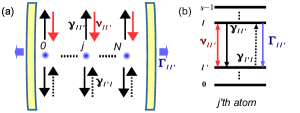
Figure 1: (a) shows identical atoms labeled by $j$ from zero to $N$ in an optical cavity. (b) shows the atomic levels labeled by $l$ from zero to $s-1$ and the involved processes. The atoms might be excited coherently with a strength $v_{ll^{\prime}}$ (red arrows), pumped incoherently with a rate $\gamma_{l^{\prime}l}$ (black dashed arrow), decay individually with a rate $\gamma_{ll^{\prime}}$ (black solid arrow) or collectively with a rate $\Gamma_{ll^{\prime}}$ (blue solid arrow, caused by the coupling with the lossy cavity). For more details see text.

In this article, we present a collective description of density matrix for identical multi-level atoms, which are either driven coherently or pumped incoherently while subject to either individual decay or collective decay, see Fig. 1 (a). In our description, we identify the group of identical matrix elements and derive the equation for the group, considered as single entity, by following a rigorous procedure. Our description removes the redundancy of matrix elements and thus is suitable for simulating superradiance from many atoms. In essence, our description generalizes the method based on flip-spin numbers (MRichter, ; Ullrich, ; MGegg, ; YZhang, ). More importantly, it allows us to explore the symmetry of density matrix (MXu, ) without explicitly applying the group theory and thus is much easy to be implemented.

As an example, we utilize our description to simulate transient and steady-state superradiance from hundreds of two-level atoms. In particular, we correlate the radiation dynamics with the atomic dynamics. We find that the superradiance without dipole appears from the atoms, which are either fully excited initially or pumped incoherently. In contrast, the superradiance with dipole (i.e. superfluorescence) appears for the atoms, which are either prepared in superposition states or driven coherently. In addition, we find that the superradiance is correlated much stronger with the uncertainty of atomic angular moment.

This article is organized as follows. In the following section, we present our description. In Sec. III we present our results on the transient and steady-state superradiance from hundreds of two-level atoms. In the end we provide some concluding remarks and comment on the possible extensions in the future.

II Collective Description of Density Matrix

In this section, we present our description for identical multi-level atoms subject to coherent driving, individual decay, pumping and collective decay, see Fig. 1 (b). Such a system is described by the master equation

$$\frac{\partial}{\partial t}\rho=\frac{1}{i\hbar}\left[H_{a}+H_{d},\rho\right]-\mathcal{D}_{d}\left[\rho\right]-\mathcal{D}_{p}\left[\rho\right]+\frac{1}{i\hbar}\left[H_{s},\rho\right]-\mathcal{D}_{c}\left[\rho\right]$$ (1)

for the density operator $\rho$. The first three terms on the right side of Eq. (1) describe the processes related to individual atoms. $H_{a}=\sum_{l=0}^{s-1}\hbar\omega_{l}\sum_{j=1}^{N}\left|l_{j}\right\rangle\left\langle l_{j}\right|$ describes the Hamiltonian of $N$ identical atoms, which are labeled by $j$ and have $s$ states (levels) $\left|l_{j}\right\rangle$ with energies $\hbar\omega_{l}$ each, see Fig. 1(b). To simplify the notion, we introduce the operator $\sigma^{j}_{ll^{\prime}}=\left|l_{j}\right\rangle\left\langle l^{\prime}_{j}\right|$ for individual atoms and then the collective operator $\sigma_{ll^{\prime}}=\sum_{j}\sigma^{j}_{ll^{\prime}}$ for the atom ensemble. As a result, we can rewrite $H_{a}$ as $\sum_{l}\hbar\omega_{l}\sigma_{ll}$. $H_{d}=\hbar\sum_{l>l^{\prime}}\left(v_{ll^{\prime}}\sigma_{ll^{\prime}}+\mathrm{h.c.}\right)$ describes the interaction between the $l-l^{\prime}$ transitions of the atoms and an external field of frequency $\omega_{d}$ with the strength $v_{ll^{\prime}}=v_{ll^{\prime}}^{0}\exp\left(-i\omega_{d}t\right)$ (in rotating-wave approximation). $\mathcal{D}_{d}\left[\rho\right]=\sum_{l\neq l^{\prime}}\frac{\gamma_{ll^{\prime}}}{2}\sum_{j}\mathcal{D}\left[\sigma_{l^{\prime}l}^{j}\right]\rho$ describes the dissipation of individual atoms, which includes either the decay from the upper level ($l>l^{\prime}$) or the incoherent pumping (DMeiser, ; DMeiser1, ) from the lower level ($l<l^{\prime}$). $\mathcal{D}_{p}\left[\rho\right]=\sum_{l>l^{\prime}}\frac{\xi_{ll^{\prime}}}{2}\sum_{j}\mathcal{D}\left[\sigma_{ll}^{j}-\sigma_{l^{\prime}l^{\prime}}^{j}\right]\rho$ describes the dephasing $\xi_{ll^{\prime}}$ between $l-l^{\prime}$ transition . Here, the superoperator is defined as $\mathcal{D}\left[o\right]=\left\{o^{+}o,\rho\right\}-2o\rho o^{+}$ (for any operator $o$).

The remaining terms on the right side of Eq. (1) are obtained by adiabatically eliminating the cavity mode from the laser master equation. The Hamiltonian $H_{s}=\sum_{l>l^{\prime}}\hbar\Omega_{ll^{\prime}}\sigma_{ll^{\prime}}\sigma_{l^{\prime}l}$ describes the collective Lamb shift of the atomic transitions $\Omega_{ll^{\prime}}=\left|g_{ll^{\prime}}\right|^{2}\chi_{ll^{\prime}}\left[\chi_{ll^{\prime}}^{2}+\left(\kappa/2\right)^{2}\right]^{-1}$and the Lindblad term $\mathcal{D}_{c}\left[\rho\right]=\sum_{l>l^{\prime}}\frac{\Gamma_{ll^{\prime}}}{2}\mathcal{D}\left[\sigma_{l^{\prime}l}\right]\rho$ describes the collective atomic decay $\Gamma_{ll^{\prime}}=\left|g_{ll^{\prime}}\right|^{2}\left(\kappa/2\right)\left[\chi_{ll^{\prime}}^{2}+\left(\kappa/2\right)^{2}\right]^{-1}$. Here, $\omega_{c},\kappa$ are the cavity mode frequency and loss rate, respectively, $\chi_{ll^{\prime}}=\omega_{l}-\omega_{l^{\prime}}-\omega_{c},g_{ll^{\prime}}$ are the frequency detuning and the coupling between the atoms and the cavity mode.

To solve the master equation (1) we introduce the product states $\left|\alpha\right\rangle\equiv\prod_{j=1}^{N}\left|l_{j}\right\rangle$ and $\left|\beta\right\rangle\equiv\prod_{j=1}^{N}\left|l^{\prime}_{j}\right\rangle$ with the sets $\alpha=\left\{l_{1},...,l_{N}\right\}$, $\beta=\left\{l^{\prime}_{1},...,l^{\prime}_{N}\right\}$ and then define the density matrix elements $\rho_{\beta\alpha}$ as the expectation value $\mathrm{tr}\left\{\rho\left|\alpha\right\rangle\left\langle\beta\right|\right\}$ of the transition ($\alpha\neq\beta$) or projection ($\alpha=\beta$) operator $\left|\alpha\right\rangle\left\langle\beta\right|$. If all the atoms are identical we expect that many elements are identical and thus do not need to consider all of them. In order to do so, we need a clever way to identify these elements. To this end we should analyze the equation for the density matrix elements $\frac{\partial}{\partial t}\rho_{\beta\alpha}=\mathrm{tr}\left\{\left(\frac{\partial}{\partial t}\rho\right)\left|\alpha\right\rangle\left\langle\beta\right|\right\}$. If we utilize the master equation (1) for $\rho$ and then cyclize the operators in the expectation values such that $\rho$ appears always on the right side, we can then rewrite the equation as $\frac{\partial}{\partial t}\rho_{\beta\alpha}=\mathrm{tr}\left\{\left(\frac{\partial}{\partial t}\left|\alpha\right\rangle\left\langle\beta\right|\right)\rho\right\}$ with an ancillary equation $\frac{\partial}{\partial t}\left|\alpha\right\rangle\left\langle\beta\right|\equiv\left(i/\hbar\right)\left[H_{a}+H_{d}+H_{s},\left|\alpha\right\rangle\left\langle\beta\right|\right]-\tilde{\mathcal{D}}_{d}\left[\left|\alpha\right\rangle\left\langle\beta\right|\right]-\tilde{\mathcal{D}}_{p}\left[\left|\alpha\right\rangle\left\langle\beta\right|\right]-\tilde{\mathcal{D}}_{c}\left[\left|\alpha\right\rangle\left\langle\beta\right|\right]$, where the latter three terms are defined with the superoperator $\tilde{\mathcal{D}}\left[o\right]=\left\{o^{+}o,\left|\alpha\right\rangle\left\langle\beta\right|\right\}-2o^{+}\left|\alpha\right\rangle\left\langle\beta\right|o$. Here, we switch $o^{+}$ and $o$ in the last term compared to $\mathcal{D}\left[o\right]$. We should not consider this equation as an equation in Heisenberg picture but should consider it only as a tool to analyze the equation for $\rho_{\beta\alpha}$.

In the ancillary equation, we encounter two kinds of terms. One kind has the form like $\sum_{j}\sigma_{ll^{\prime}}^{j}\left|\alpha\right\rangle\left\langle\beta\right|,\left|\alpha\right\rangle\left\langle\beta\right|\sum_{j}\sigma_{ll^{\prime}}^{j}$ while another kind has the form like $\sum_{j}\sigma_{ll^{\prime}}^{j}\left|\alpha\right\rangle\left\langle\beta\right|\sigma_{l^{\prime}l}^{j}$. Using the identity operator $\sum_{k}\sigma_{kk}^{j}$ we can always write the first kind as a sum of the second kind. In general, we should evaluate the sandwich structure $\sum_{j}\sigma_{ll^{\prime}}^{j}\left|\alpha\right\rangle\left\langle\beta\right|\sigma_{kk^{\prime}}^{j}$. We can do so in two steps. First, we evaluate whether the $j$’th atom is on the state $\left|l^{\prime}_{j}\right\rangle$ (from $\sigma_{ll^{\prime}}^{j}$) in the product state $\left|\alpha\right\rangle$ and simultaneously on the state $\left|k_{j}\right\rangle$ (from $\sigma_{kk^{\prime}}^{j}$) in the product state $\left|\beta\right\rangle$. Second, if the evaluation turns out to be true, we replace $\left|l^{\prime}_{j}\right\rangle$ by $\left|l_{j}\right\rangle$ in $\left|\alpha\right\rangle$ and $\left|k_{j}\right\rangle$ by $\left|k^{\prime}_{j}\right\rangle$ in $\left|\beta\right\rangle$ to obtain two new product states $\left|\alpha^{\prime}\right\rangle$ and $\left|\beta^{\prime}\right\rangle$ , which form a new transition or projection operator $\left|\alpha^{\prime}\right\rangle\left\langle\beta^{\prime}\right|$. If we repeat the two steps for all the atoms, we obtain $n_{l^{\prime}k}$ terms, where $n_{l^{\prime}k}$ are the number of atoms fulfilling the evaluation in the first step. If all the atoms are identical, we expect the following relation for the expectation values

$${\rm tr}\{\rho\sum_{j}\sigma_{ll^{\prime}}^{j}\left|\alpha\right\rangle\left\langle\beta\right|\sigma_{kk^{\prime}}^{j}\}={\rm tr}\{\rho n_{ll^{\prime}}\left|\alpha^{\prime}\right\rangle\left\langle\beta^{\prime}\right|\}.$$ (2)

To facilitate the following derviation, we can ignore the trace and the density operator temporarily and assume a relation for the operators

$$\sum_{j}\sigma_{ll^{\prime}}^{j}\left|\alpha\right\rangle\left\langle\beta\right|\sigma_{kk^{\prime}}^{j}=n_{ll^{\prime}}\left|\alpha^{\prime}\right\rangle\left\langle\beta^{\prime}\right|.$$ (3)

Figure 2: Mapping of projection or transition operators $\left|\alpha\right\rangle\left\langle\beta\right|$ to single operators $\left\lceil n\right\rfloor$ (a) and three kinds of actions of the superoperators on these operators $\left\lceil n\right\rfloor$ (b,c,d) for the exemplary system with five identical two-level atoms. For more details, see the text.

If we apply Eq. (3) to those operators $\left|\alpha\right\rangle\left\langle\beta\right|$, which lead to the elements $\rho_{\beta\alpha}$ with same value, we encounter several integers $n_{ll^{\prime}}$ ($l,l^{\prime}=0,...s-1$). In other words, the set of integers $\left\{n_{ll^{\prime}}\right\}$ specify uniquely the group (or set) of operators $\left\{\left|\alpha\right\rangle\left\langle\beta\right|\right\}$, where the members $\left|\alpha\right\rangle\left\langle\beta\right|$ are affected in the same way by the sandwich structures (and thus the equation $\frac{\partial}{\partial t}\left|\alpha\right\rangle\left\langle\beta\right|$). Using this finding we can remove the redundancy of matrix elements. In the following, we present a rigorous procedure for doing so.

The core of our procedure is to define an operator $\left\lceil n\right\rfloor$ with the set of integers $n\equiv\left\{n_{ll^{\prime}}\right\}$ to represent any member of the group $\left\{\left|\alpha\right\rangle\left\langle\beta\right|\right\}$. In other words, we establish a many-to-one mapping

$$\left|\alpha\right\rangle\left\langle\beta\right|\leftrightarrow\left\lceil n\right\rfloor=\left\lceil\begin{array}[]{ccc}n_{s-1s-1}&\cdots&n_{s0}\\ \vdots&\ddots&\vdots\\ n_{0s}&\cdots&n_{00}\end{array}\right\rfloor.$$ (4)

Fig. 2(a) shows one example of the mapping for two-level atoms. Here, we choose the matrix-like form $\left\lceil\right\rfloor$ to reflect $\left\lceil n\right\rfloor$ as operators in Hilbert space. Furthermore, we can define the expectation value $\left\langle n\right\rangle\equiv\mathrm{tr}\left\{\rho\left\lceil n\right\rfloor\right\}$ and then establish a similar mapping between the matrix elements $\rho_{\beta\alpha}$ and $\left\langle n\right\rangle$. If we replace $\left|\alpha\right\rangle\left\langle\beta\right|$ with $\left\lceil n\right\rfloor$ in the ancillary equation $\frac{\partial}{\partial t}\left|\alpha\right\rangle\left\langle\beta\right|$ and then take a trace after multiplying with $\rho$, i.e. $\left\langle\cdot\right\rangle=\mathrm{tr}\left\{\rho\cdot\right\}$, on both sides, we get the following equation for $\left\langle n\right\rangle$:

$$\frac{\partial}{\partial t}\left\langle n\right\rangle=\left(i/\hbar\right)\left\langle\left[H_{a}+H_{d}+H_{s},\left\lceil n\right\rfloor\right]\right\rangle$$

$$-\sum_{l\neq l^{\prime}}\frac{\gamma_{ll^{\prime}}}{2}\Bigl{\langle}\left\{\sigma_{ll},\left\lceil n\right\rfloor\right\}-2\sum_{j}\sigma_{ll^{\prime}}^{j}\left\lceil n\right\rfloor\sigma_{l^{\prime}l}^{j}\Bigr{\rangle}$$

$$-\sum_{l>l^{\prime}}\frac{\xi_{ll^{\prime}}}{2}\Bigl{\langle}\left\{\sigma_{ll}-\sigma_{l^{\prime}l^{\prime}},\left\lceil n\right\rfloor\right\}-2\sum_{j}\left(\sigma_{ll}^{j}-\sigma_{l^{\prime}l^{\prime}}^{j}\right)\left\lceil n\right\rfloor\left(\sigma_{ll}^{j}-\sigma_{l^{\prime}l^{\prime}}^{j}\right)\Bigr{\rangle}$$

$$-\sum_{l>l^{\prime}}\frac{\Gamma_{ll^{\prime}}}{2}\Bigl{\langle}\Bigl{\{}\sigma_{ll^{\prime}}\sigma_{l^{\prime}l},\left\lceil n\right\rfloor\Bigr{\}}-2\sigma_{ll^{\prime}}\left\lceil n\right\rfloor\sigma_{l^{\prime}l}\Bigr{\rangle}.$$ (5)

In the second line, we have utilized $\sigma_{ll^{\prime}}^{j}\sigma_{l^{\prime}l}^{j}=\sigma_{ll}^{j}$ and $\sigma_{ll}=\sum_{j}\sigma_{ll}^{j}$. Since $\left\langle n\right\rangle$ represents the group of $\rho_{\beta\alpha}$ of same value, we might call it as collective density matrix. In the following, we evaluate the different terms in the above equation.

II.1 Contributions to Collective Density Matrix Equation

To evaluate the contribution $\left(\frac{\partial}{\partial t}\left\langle n\right\rangle\right)_{a}$ of $H_{a}$ in Eq. (5), we encounter two terms $\sigma_{ll}\left\lceil n\right\rfloor$,$\left\lceil n\right\rfloor\sigma_{ll}$. To evaluate them we consider $\left\lceil n\right\rfloor$ as a vector in Liouville space and promote $\sigma_{ll}$ as a superoperator, which can act on $\left\lceil n\right\rfloor$ either from the left side $\sigma_{ll}\left\lceil n\right\rfloor$ or from the right side $\left\lceil n\right\rfloor\sigma_{ll}$. As an example, we demonstrate the evaluation of $\sigma_{ll}\left\lceil n\right\rfloor$ . Using the identity operator $\sum_{k}\sigma_{kk}^{j}$ of the $j$’th atom, we can rewrite $\sigma_{ll}\left\lceil n\right\rfloor$ as $\sum_{k}\sum_{j}\sigma_{ll}^{j}\left\lceil n\right\rfloor\sigma_{kk}^{j}.$ Here, we have expanded $\sigma_{ll}$ as $\sum_{j}\sigma_{ll}^{j}$. To proceed, we turn $\left\lceil n\right\rfloor$ back to $\left|\alpha\right\rangle\left\langle\beta\right|$ and then apply Eq. (3) to obtain $\sum_{j}\sigma_{ll}^{j}\left|\alpha\right\rangle\left\langle\beta\right|\sigma_{kk}^{j}=n_{lk}\left|\alpha\right\rangle\left\langle\beta\right|$. Notice that the product states do not change on the right side. Using the mapping of Eq. (4), we obtain

$$\sum_{j}\sigma_{ll}^{j}\left\lceil n\right\rfloor\sigma_{kk}^{j}=n_{lk}\left\lceil n\right\rfloor.$$ (6)

This relation is exemplified with Fig. 2 (b) for two-level atoms. If we sum up the above relations for different $k$, we obtain

$$\sigma_{ll}\left\lceil n\right\rfloor=\sum_{l^{\prime}}n_{ll^{\prime}}\left\lceil n\right\rfloor.$$ (7)

We can follow the same procedure to evaluate $\left\lceil n\right\rfloor\sigma_{ll}$. Notice that this time we should apply the identity operator from the left side. As a result, we should obtain

$$\left\lceil n\right\rfloor\sigma_{ll}=\sum_{l^{\prime}}n_{l^{\prime}l}\left\lceil n\right\rfloor.$$ (8)

Using the above expressions, we finally get the contribution of $H_{a}$ to the master equation

$$\left(\frac{\partial}{\partial t}\left\langle n\right\rangle\right)_{a}=i\sum_{l}\omega_{l}\sum_{l^{\prime}}\left(n_{ll^{\prime}}-n_{l^{\prime}l}\right)\left\langle n\right\rangle.$$ (9)

To evaluate the contribution $\left(\frac{\partial}{\partial t}\left\langle n\right\rangle\right)_{d}$ of $H_{d}$ in Eq. (5), we have to evaluate the action of $\sigma_{ll^{\prime}}$ ($l\neq l^{\prime}$) on $\left\lceil n\right\rfloor$ from the left side $\sigma_{ll^{\prime}}\left\lceil n\right\rfloor$ and from the right side $\left\lceil n\right\rfloor\sigma_{ll^{\prime}}$. As an example, we detail the evalulation of $\sigma_{ll^{\prime}}\left\lceil n\right\rfloor$. Using the identity operator of the $j$-th atom, we can rewrite this term as $\sum_{k}\sum_{j}\sigma_{ll^{\prime}}^{j}\left\lceil n\right\rfloor\sigma_{kk}^{j}$. To evaluate the terms inside the sum to $k$, we can turn $\left\lceil n\right\rfloor$ back to $\left|\alpha\right\rangle\left\langle\beta\right|$ and then apply Eq. (3) to obtain $\sum_{j}\sigma_{ll^{\prime}}^{j}\left|\alpha\right\rangle\left\langle\beta\right|\sigma_{kk}^{j}=n_{l^{\prime}k}\left|\alpha^{\prime}\right\rangle\left\langle\beta\right|$. Notice that the product state $\left|\beta\right\rangle$ does not change on the right side. The product state $\left|\alpha^{\prime}\right\rangle$ differs from $\left|\alpha\right\rangle$ by that one of the atoms, which is initially on $\left|l^{\prime}\right\rangle$ state, is now on $\left|l\right\rangle$ state. Using the mapping of Eq. (4), we can map $\left|\alpha^{\prime}\right\rangle\left\langle\beta\right|$ to a new operator $\left\lceil n^{\prime}\right\rfloor$, which differs from $\left\lceil n\right\rfloor$ by that $n_{l^{\prime}k}$ reduces by one and $n_{lk}$ increases by one. To sum up, we establish the following relation

$$\sigma_{ll^{\prime}}\left\lceil n\right\rfloor =\sum_{k}n_{l^{\prime}k}\left\lceil\left\{n_{l^{\prime}k}-1,n_{lk}+1\right\}\right\rfloor.$$ (10)

Here and in the following, for simplicity, we indicate the new operator $\left\lceil n^{\prime}\right\rfloor$ with only the changed numbers relative to $\left\lceil n\right\rfloor$. Fig. 2(c) shows one example of the above relation for two-level atoms. Following the same procedure, we can also get

$$\left\lceil n\right\rfloor\sigma_{ll^{\prime}} =\sum_{k}n_{kl}\left\lceil\left\{n_{kl}-1,n_{kl^{\prime}}+1\right\}\right\rfloor.$$ (11)

Using the above expressions we get the contribution of $H_{d}$ to the master equation

$$\left(\frac{\partial}{\partial t}\left\langle n\right\rangle\right)_{d}=$$

$$i\sum_{l\neq l^{\prime}}v_{ll^{\prime}}\sum_{k}\left(n_{l^{\prime}k}\left\langle n_{l^{\prime}k}-1,n_{lk}+1\right\rangle-n_{kl}\left\langle n_{kl}-1,n_{kl^{\prime}}+1\right\rangle\right)$$

$$+i\sum_{l\neq l^{\prime}}v_{ll^{\prime}}^{*}\sum_{k}\left(n_{lk}\left\langle n_{lk}-1,n_{l^{\prime}k}+1\right\rangle-n_{kl^{\prime}}\left\langle n_{kl^{\prime}}-1,n_{kl}+1\right\rangle\right).$$ (12)

To evaluate the contribution $\left(\frac{\partial}{\partial t}\left\langle n\right\rangle\right)_{s}$ of $H_{s}$ in Eq. (5), we have to evaluate the action of $\sigma_{ll^{\prime}}\sigma_{l^{\prime}l}$ ($l\neq l^{\prime}$) on $\left\lceil n\right\rfloor$ from the left side $\sigma_{ll^{\prime}}\sigma_{l^{\prime}l}\left\lceil n\right\rfloor$ and from the right side $\left\lceil n\right\rfloor\sigma_{ll^{\prime}}\sigma_{l^{\prime}l}$. To evaluate these terms we apply simply Eq. (10) and (11) twice to obtain

$$\sigma_{ll^{\prime}}\sigma_{l^{\prime}l}\left\lceil n\right\rfloor=\sum_{k}n_{lk}\left(n_{l^{\prime}k}+1\right)\left\lceil n\right\rfloor$$

$$+\sum_{k\neq k^{\prime}}n_{lk}n_{l^{\prime}k^{\prime}}\left\lceil\left\{n_{lk}-1,n_{l^{\prime}k^{\prime}}-1,n_{l^{\prime}k}+1,n_{l^{\prime}k^{\prime}}+1\right\}\right\rfloor,$$ (13)

$$\left\lceil n\right\rfloor\sigma_{ll^{\prime}}\sigma_{l^{\prime}l}=\sum_{k}n_{kl}\left(n_{kl^{\prime}}+1\right)\left\lceil n\right\rfloor$$

$$+\sum_{k\neq k^{\prime}}n_{kl}n_{k^{\prime}l^{\prime}}\left\lceil\left\{n_{kl}-1,n_{k^{\prime}l^{\prime}}-1,n_{kl^{\prime}}+1,n_{k^{\prime}l}+1\right\}\right\rfloor.$$ (14)

Notice that the operators in the second and fourth line differ from $\left\lceil n\right\rfloor$ by four numbers as indicated. Using these expressions we obtain

$$\left(\frac{\partial}{\partial t}\left\langle n\right\rangle\right)_{s}=i\sum_{l>l^{\prime}}\Omega_{ll^{\prime}}\Bigl{[}\sum_{k}\left(n_{lk}\left(n_{l^{\prime}k}+1\right)-n_{kl}\left(n_{kl^{\prime}}+1\right)\right)\left\langle n\right\rangle$$

$$+\sum_{k\neq k^{\prime}}n_{lk}n_{l^{\prime}k^{\prime}}\left\langle n_{lk}-1,n_{l^{\prime}k^{\prime}}-1,n_{l^{\prime}k}+1,n_{l^{\prime}k^{\prime}}+1\right\rangle$$

$$-\sum_{k\neq k^{\prime}}n_{kl}n_{k^{\prime}l^{\prime}}\left\langle n_{kl}-1,n_{k^{\prime}l^{\prime}}-1,n_{kl^{\prime}}+1,n_{k^{\prime}l}+1\right\rangle\Bigr{]}.$$ (15)

To evaluate the contribution $\left(\frac{\partial}{\partial t}\left\langle n\right\rangle\right)_{d}$ of the individual dissipation $\mathcal{D}_{d}\left[\rho\right]$ in Eq. (5), we encounter $\sigma_{ll}\left\lceil n\right\rfloor,\left\lceil n\right\rfloor\sigma_{ll}$ and $\sum_{j}\sigma_{ll^{\prime}}^{j}\left\lceil n\right\rfloor\sigma_{l^{\prime}l}^{j}$ . Since the former two expressions can be evaluated with Eq. (7) and (8), we focus on the last term. In the same spirit as before, we turn $\left\lceil n\right\rfloor$ back to $\left|\alpha\right\rangle\left\langle\beta\right|$ and then apply Eq. (3) to obtain $\sum_{j}\sigma_{ll^{\prime}}^{j}\left|\alpha\right\rangle\left\langle\beta\right|\sigma_{l^{\prime}l}^{j}=n_{l^{\prime}l^{\prime}}\left|\alpha^{\prime}\right\rangle\left\langle\beta^{\prime}\right|$. Here, the new product state $\left|\alpha^{\prime}\right\rangle$ ($\left|\beta^{\prime}\right\rangle$) differs from $\left|\alpha\right\rangle$ ($\left|\beta\right\rangle$) by that one of the atoms, which is on $\left|l^{\prime}\right\rangle$ state in $\left|\alpha\right\rangle$ ($\left|\beta\right\rangle$), is now on $\left|l\right\rangle$ state. Using the mapping of Eq. (4), we map $\left|\alpha^{\prime}\right\rangle\left\langle\beta^{\prime}\right|$ to a new operator $\left\lceil n^{\prime}\right\rfloor$, which differs from $\left\lceil n\right\rfloor$ by that $n_{l^{\prime}l^{\prime}}$ reduces by one and $n_{ll}$ increases by one. To sum up, we establish the following relation

$$\sum_{j}\sigma_{ll^{\prime}}^{j}\left\lceil n\right\rfloor\sigma_{l^{\prime}l}^{j}=n_{l^{\prime}l^{\prime}}\left\lceil\left\{n_{l^{\prime}l^{\prime}}-1,n_{ll}+1\right\}\right\rfloor.$$ (16)

This relation is exemplified with Fig. 2(d) for two-level atoms. With the above expression and also Eqs. (7) and (8) we get

$$\left(\frac{\partial}{\partial t}\left\langle n\right\rangle\right)_{d}=\sum_{l\neq l^{\prime}}\frac{\gamma_{ll^{\prime}}}{2}\Bigl{[}\sum_{k}\left(n_{lk}+n_{kl}\right)\left\langle n\right\rangle-2n_{l^{\prime}l^{\prime}}\left\langle n_{l^{\prime}l^{\prime}}-1,n_{ll}+1\right\rangle\Bigr{]}.$$ (17)

To evaluate the contribution $\left(\frac{\partial}{\partial t}\left\langle n\right\rangle\right)_{p}$ of the individual dephasing $\mathcal{D}_{p}\left[\rho\right]$ in Eq. (5), we encounter the terms $\sigma_{ll}\left\lceil n\right\rfloor,\left\lceil n\right\rfloor\sigma_{ll}$,$\sum_{j}\sigma_{ll}^{j}\left\lceil n\right\rfloor\sigma_{ll}^{j},\sum_{j}\sigma_{ll}^{j}\left\lceil n\right\rfloor\sigma_{l^{\prime}l^{\prime}}^{j}$ (also terms with $l,l^{\prime}$ exchanged). The former two terms can be evaluated with Eq. (7) and (8). The latter two terms can be evaluated with Eq. (6). As a result, we get

$$\left(\frac{\partial}{\partial t}\left\langle n\right\rangle\right)_{p} =-\sum_{l>l^{\prime}}\frac{\xi_{ll^{\prime}}}{2}\Bigl{[}\sum_{k}\left(n_{lk}+n_{kl}-n_{l^{\prime}k}-n_{kl^{\prime}}\right)$$

$$-2\left(n_{ll}-n_{ll^{\prime}}-n_{l^{\prime}l}+n_{l^{\prime}l^{\prime}}\right)\Bigr{]}\left\langle n\right\rangle.$$ (18)

To evaluate the contribution $\left(\frac{\partial}{\partial t}\left\langle n\right\rangle\right)_{c}$ of the collective decay $\mathcal{D}_{c}\left[\rho\right]$ in Eq. (5) we encounter three terms $\sigma_{ll^{\prime}}\sigma_{l^{\prime}l}\left\lceil n\right\rfloor$, $\left\lceil n\right\rfloor\sigma_{ll^{\prime}}\sigma_{l^{\prime}l}$ and $\sigma_{l^{\prime}l}\left\lceil n\right\rfloor\sigma_{ll^{\prime}}$. To evaluate the former two terms, we can simply apply Eq. (10) and (11) twice to get Eq. (13) and 14. In order to evaluate the last term, we apply Eq. (10) and (11) once to get

$$\sigma_{ll^{\prime}}\left\lceil n\right\rfloor\sigma_{l^{\prime}l}=n_{l^{\prime}l^{\prime}}\left(n_{l^{\prime}l}+1\right)\left\lceil\left\{n_{l^{\prime}l^{\prime}}-1,n_{ll}+1\right\}\right\rfloor$$

$$+\sum_{k\neq l^{\prime},k^{\prime}\neq l}n_{kl^{\prime}}n_{l^{\prime}k^{\prime}}\left\lceil\left\{n_{kl^{\prime}}-1,n_{l^{\prime}k^{\prime}}-1,n_{kl}+1,n_{lk^{\prime}}+1\right\}\right\rfloor.$$ (19)

With the above expressions, we finally obtain

$$\left(\frac{\partial}{\partial t}\left\langle n\right\rangle\right)_{c}=-\sum_{l>l^{\prime}}\frac{\Gamma_{ll^{\prime}}}{2}\Bigl{\{}\sum_{k}\left[n_{lk}\left(n_{l^{\prime}k}+1\right)+n_{kl}\left(n_{kl^{\prime}}+1\right)\right]\left\langle n\right\rangle$$

$$+\sum_{k\neq k^{\prime}}\Bigl{(}n_{lk}n_{l^{\prime}k^{\prime}}\left\langle n_{lk}-1,n_{l^{\prime}k^{\prime}}-1,n_{l^{\prime}k}+1,n_{l^{\prime}k^{\prime}}+1\right\rangle$$

$$+n_{kl}n_{k^{\prime}l^{\prime}}\left\langle n_{kl}-1,n_{k^{\prime}l^{\prime}}-1,n_{kl^{\prime}}+1,n_{k^{\prime}l}+1\right\rangle\Bigr{)}$$

$$-2\Bigl{[}n_{l^{\prime}l^{\prime}}\left(n_{l^{\prime}l}+1\right)\left\langle n_{l^{\prime}l^{\prime}}-1,n_{ll}+1\right\rangle$$

$$+\sum_{k\neq l^{\prime},k^{\prime}\neq l}n_{kl^{\prime}}n_{l^{\prime}k^{\prime}}\left\langle n_{kl^{\prime}}-1,n_{l^{\prime}k^{\prime}}-1,n_{kl}+1,n_{lk^{\prime}}+1\right\rangle\Bigr{]}\Bigr{\}}.$$ (20)

II.2 Initial Conditions and Observables

In the above subsection, we have obtained self-consistent equation for the collective density matrix $\left\langle n\right\rangle$. To solve this equation, we have to also specify the initial condition. In general, the initial states of individual atoms can be mixed states and thus should be specified by a set of pure states $\left\{\left|\psi_{i}\right\rangle_{j}\right\}$ and a set of probabilities $\left\{m_{i}\right\}$ (satisfying $\sum_{i}m_{i}=1$). From the two sets we obtain the initial density operator $\rho_{0,j}\equiv\sum_{i}m_{i}\left|\psi_{i}\right\rangle_{j}\left\langle\psi_{i}\right|_{j}$ of the $j$’th atom. The pure states $\left|\psi_{i}\right\rangle_{j}$ can be specified as $\left|\psi_{i}\right\rangle_{j}=\sum_{l}c_{l}^{i}\left|l_{j}\right\rangle$ with complex numbers $c_{j}^{i}$ (fulfilling the condition $\sum_{l}\left|c_{l}^{i}\right|^{2}=1$). Here, we assume that $m_{i}$ and $c_{l}^{i}$ do not depend on the specific atoms. If there is no any correlation between the atoms, we can obtain the initial density operator of all the atoms with the direct product $\rho_{0}=\prod_{j}\rho_{0,j}$.

To proceed, we insert the definition of $\rho_{0,j}$ to $\rho_{0}$ and then combine the states $\bigl{|}l_{j}\bigr{\rangle}$ ($\bigl{\langle}l^{\prime}_{j}\bigr{|}$) on the left (right) side to form the product states $\left|\beta\right\rangle$ ($\left\langle\alpha\right|$), and then map the operator $\left|\beta\right\rangle\left\langle\alpha\right|$ to the operator $\left\lceil n\right\rfloor$. As a result, we get the initial density operator of the atoms

$$\rho_{0}=\sum_{\left\{n_{ll^{\prime}}\right\}}C_{\left\{n_{ll^{\prime}}\right\}}\prod_{l,l^{\prime}}\left(\sum_{i}m_{i}c_{l}^{i}c_{l^{\prime}}^{i*}\right)^{n_{ll^{\prime}}}\left\lceil n\right\rfloor.$$ (21)

Here, $\sum_{\left\{n_{ll^{\prime}}\right\}}$ indicates the sum to those $n_{ll^{\prime}}$ satisfying the relation $\sum_{ll^{\prime}}n_{ll^{\prime}}=N$. $C_{\left\{n_{ll^{\prime}}\right\}}$ is the number of $\left|\beta\right\rangle\left\langle\alpha\right|$ mapped to the same $\left\lceil n\right\rfloor$. With the above expression, we can obtain the initial condition for the collective density matrix $\left\langle n\right\rangle_{0}=\mathrm{tr}\left\{\rho_{0}\left\lceil n\right\rfloor\right\}$:

$$\left\langle n\right\rangle_{0}=\prod_{l,l^{\prime}=0}^{s-1}\left(\sum_{i}m_{i}c_{l}^{i}c_{l^{\prime}}^{i*}\right)^{n_{ll^{\prime}}}.$$ (22)

Once we solve the equation for the collective density matrix, we would like to analyze the system dynamics. To this end, we have to compute the observable of interest. In general, the observable is expectation value $\left\langle O\right\rangle=\mathrm{tr}\left\{O\rho\right\}$ of a collective operator $O=\sum_{j}o_{j}$. Using the identity operator $\sum_{\alpha}\left|\alpha\right\rangle\left\langle\alpha\right|$, we can rewrite the observable as $\left\langle O\right\rangle=\mathrm{tr}\left\{O\sum_{\alpha}\left|\alpha\right\rangle\left\langle\alpha\right|\rho\right\}$. To proceed, we consider the mapping of the projection operator

$$\left|\alpha\right\rangle\left\langle\alpha\right|\leftrightarrow\left\lceil\left\{n_{ll}\right\}\right\rfloor\equiv\left\lceil\begin{array}[]{ccc}n_{s-1s-1}&0&0\\ 0&\ddots&0\\ 0&0&n_{00}\end{array}\right\rfloor.$$ (23)

Here, $n_{ll}$ denotes the number of atoms on the $\left|l\right\rangle$ states in the product states $\left|\alpha\right\rangle$. Notice that the numbers $n_{ll^{\prime}}$ with $l\neq l^{\prime}$ are zero. To simplify the notation we utilize $\left\lceil\left\{n_{ll}\right\}\right\rfloor$ to represent this specific operator. Using the same argument as applied to obtain Eq. (21), we can obtain the relation

$$\sum_{\alpha}\left|\alpha\right\rangle\left\langle\alpha\right|=\sum_{\left\{n_{ll}\right\}}C_{\left\{n_{ll}\right\}}\left\lceil\left\{n_{ll}\right\}\right\rfloor,$$ (24)

where $\sum_{\left\{n_{ll}\right\}}$ is the sum to $n_{ll}$ satisfying $\sum_{l}n_{ll}=N$ and $C_{\left\{n_{ll}\right\}}=\prod_{k=0}^{s-1}C_{N-\sum_{l=0}^{k-1}n_{ll}}^{n_{kk}}$ is defined with the binomial function $C_{n}^{m}=n!/\left[m!\left(n-m\right)!\right]$. This expression allows us to rewrite the observable as

$$\left\langle O\right\rangle=\sum_{\left\{n_{ll}\right\}}C_{\left\{n_{ll}\right\}}\left\langle O\left\lceil\left\{n_{ll}\right\}\right\rfloor\right\rangle.$$ (25)

Setting $O=\sigma_{ll}$ in Eq. (25) and using Eq. (7 we obtain the population of the $\left|l\right\rangle$ states $P_{l}\equiv\sum_{\left\{n_{ll}\right\}}C_{\left\{n_{ll}\right\}}n_{ll}\left\langle\left\{n_{ll}\right\}\right\rangle$. Setting $O=\sigma_{ll^{\prime}}$ and using Eq. (10) we obtain the polarization $C_{ll^{\prime}}$ of the $l-l^{\prime}$ transition $C_{ll^{\prime}}\equiv\sum_{\left\{n_{ll}\right\}}C_{\left\{n_{ll}\right\}}n_{l^{\prime}l^{\prime}}\left\langle\left\{n_{l^{\prime}l^{\prime}}-1,n_{ll^{\prime}}+1\right\}\right\rangle.$

If we drive the atoms coherently or pump them incoherently, we arrive at steady-state. In this case, we can calculate the steady-state spectrum of the atoms $S\left(\omega\right)$. According to quantum regression theorem (PMeystre, ), we have $S\left(\omega\right)\propto\sum_{l>l^{\prime}}\Gamma_{ll^{\prime}}\textrm{Re}\int_{0}^{\infty}d\tau e^{-i\omega\tau}\mathrm{tr}\left\{\sigma_{ll^{\prime}}\tilde{\rho}\left(\tau\right)\right\}$ with the operator $\tilde{\rho}\left(\tau\right)$, which satisfies the master equation as $\rho$ with however the initial condition $\sigma_{l^{\prime}l}\rho_{std}$, where $\rho_{std}$ is the density operator at the steady-state. Furthermore, we can utilize Eq. (24) to rewrite the expression inside the integral as $\mathrm{tr}\left\{\sigma_{ll^{\prime}}\tilde{\rho}\left(\tau\right)\right\}=\sum_{\left\{n_{kk}\right\}}C_{\left\{n_{kk}\right\}}n_{l^{\prime}k}\left\langle\left\{n_{kk}-1,n_{lk}=1\right\}\right\rangle_{\tilde{\rho}\left(\tau\right)}.$ Here, we have used Eq. (10) and introduced the function $\left\langle n\right\rangle_{\tilde{\rho}\left(\tau\right)}=\mathrm{tr}\left\{\left\lceil n\right\rfloor\tilde{\rho}\left(\tau\right)\right\}$. The term on the right side differs from $\left\langle\left\{n_{kk}\right\}\right\rangle_{\tilde{\rho}\left(\tau\right)}$ by that $n_{kk}$ reduces by one and $n_{lk}$ becomes one. The function $\left\langle n\right\rangle_{\tilde{\rho}\left(\tau\right)}$ satisfies the same equation as $\left\langle n\right\rangle$ with however the initial condition $\left\langle n\right\rangle_{\tilde{\rho}\left(0\right)}=\sum_{k}n_{kl^{\prime}}\left\langle\left\{n_{kl^{\prime}}-1,n_{kl}+1\right\}\right\rangle_{std}$. We obtain this condition with the help of Eq. (11). By integrating the spectrum with respect to the frequency, we obtain the radiation intensity $I=I_{ind}+I_{c}$, which includes the contribution from individual atoms $I_{ind}\propto\sum_{l>l^{\prime}}\Gamma_{ll^{\prime}}C_{\left\{n_{ll}\right\}}n_{ll}\left\langle\left\{n_{ll}\right\}\right\rangle_{std}$ and from the atomic correlation $I_{c}\propto\sum_{l>l^{\prime}}\Gamma_{ll^{\prime}}C_{\left\{n_{ll}\right\}}n_{ll}n_{l^{\prime}l^{\prime}}\left\langle n_{ll}-1,n_{l^{\prime}l^{\prime}}-1,n_{l^{\prime}l}=1,n_{l^{\prime}l^{\prime}}=1\right\rangle_{std}$. Here, we have utilized Eq. (13) and (24). Notice that $I_{c}$ is determined by the off-diagonal elements of $\left\langle n\right\rangle$.

II.3 Numerical Implementation and Complexity Analysis

In the following, we discuss how to solve the equation for $\left\langle n\right\rangle$ numerically. To this end, we should first find an efficient way of representing $\left\langle n\right\rangle$ in the computer. In principle, we can view $\left\langle n\right\rangle$ as a matrix with $s^{2}$ dimensions and $N$ elements for each dimension. In this case, the matrix is a very sparse because the elements satisfying $\sum_{\left\{n_{ll^{\prime}}\right\}}n_{ll^{\prime}}\neq N$ are not necessary. In practice, we can define an one-dimensional array to represent only the $N_{dm}$ (specified later on) necessary elements $\left\langle n\right\rangle$. Then, the remaining question is how to relate the index of elements $i$ with the set of numbers $\left\{n_{ll^{\prime}}\right\}$. The easy solution is to define a $N_{dm}\times s^{2}$ two-dimensional ancillary array, where the first dimension specifies $i$ and the second dimension the values $\left\{n_{ll^{\prime}}\right\}$. To reduce the size of the ancillary array, we need a clever way to compress this array. We propose to compress the set $\left\{n_{ll^{\prime}}\right\}$ to single number $n_{i}$ with the relation $n_{i}=\sum_{l,l^{\prime}=0}^{s-1}\left(N^{s\times l+l^{\prime}}+n_{ll^{\prime}}\right)$. Then, we can use the index $i$ of $\left\langle n\right\rangle$ to retrieve $n_{i}$ from the ancillary array and then obtain $n_{ll^{\prime}}$ by dividing $n_{i}$ sequentially with the power of $N$ and taking the residual. In return, if we know $n_{ll^{\prime}}$, we can calculate $n_{i}$ with the expression given above and then locate the position $i$ of $n_{i}$ in the integer array and finally utilize $i$ to find the required $\left\langle n\right\rangle$.

The above discussion indicates that the complexity of solving the equation numerically is mainly determined by the number $N_{dm}$ of the elements $\left\langle n\right\rangle=\mathrm{tr}\left\{\rho\left\lceil n\right\rfloor\right\}$. To compute this number, we recall that $\left\lceil n\right\rfloor$ are specified by a set of numbers $\left\{n_{ll^{\prime}}\right\}$ under the restriction $\sum_{l,l^{\prime}}n_{ll^{\prime}}=N$. If we image the atoms as $N$ balls and $n_{ll^{\prime}}$ the number of balls in the box labeled by $ll^{\prime}$, the searched number is equivalent to the number of possibilities of arranging $N$ balls in the boxes. After some calculation, we get the number $N_{dm}=C_{N+s^{2}-1}^{s^{2}-1}$ and can approximate it as $N^{s^{2}-1}$. We see that this number increases polynomially with the number of atoms $N$ but exponentially with the number $s$ of levels. As an example, the number is estimated as $N^{3},N^{8},N^{15}$ for $N$ two-, three- and four-level atoms, respectively. We estimate this number as $1.5\times 10^{7}$ for $250$ two-, $25$ three- or $12$ four-level atoms and thus we need about $5$ Gb memory to represent $\left\langle n\right\rangle$ in the computer if we assume $2$ bits for one element. This simple calculation establishes the maximum number of atoms that can be simulated with a normal computer.

III Superradiance of Hundreds of Two-level atoms

In this section, we apply our collective description of density matrix to two-level atoms by simply restricting the level indices $l,l^{\prime}$ to zero (lower level) and one (upper level) and study the superradiance from hundreds of atoms, which are either initially excited, coherently driven or incoherently pumped. To understand the results, we should keep in mind that $\gamma_{10},\gamma_{01},\xi_{10}$ are the decay, pumping and dephasing rate of individual atoms while $\Gamma_{10}$ is the collective decay rate.

As explained in the introduction, this system is often described by the superradiance master equation, which is defined with the collective Pauli operator $\sigma_{z}=\sum_{j}\sigma_{z}^{j}$ and the collective creation $\sigma_{\text{+}}=\sum_{j}\sigma_{\text{+}}^{j}$ and annihilation ladder operator $\sigma_{-}=\sum_{j}\sigma_{-}^{j}$. This description is equivalent to our description because of $\sigma_{z}^{j}=\sigma_{11}^{j}-\sigma_{00}^{j}$, $\sigma_{\text{+}}^{j}=\sigma_{10}^{j}$ and $\sigma_{-}^{j}=\sigma_{01}^{j}$. In addition, the description with $\sigma_{z},\sigma_{\pm}$ also implies that the two-level atoms are equivalent to spin-1/2 particles. Thus, we can also introduce the spin operator $j_{x}=\left(\sigma_{-}+\sigma_{+}\right)/2,j_{y}=i\left(\sigma_{-}-\sigma_{+}\right)/2,j_{z}=\sigma_{z}/2$ and visualize the atomic dynamics with angular moment $\mathbf{J}=\sum_{i=x,y,z}J_{i}\mathbf{e}_{i}$ and their uncertainty $\Delta\mathbf{J}=\sum_{i}\Delta J_{i}\mathbf{e}_{i}$, where $J_{i}=\left\langle j_{i}\right\rangle$ and $\Delta J_{i}=\sqrt{\left\langle j_{i}^{2}\right\rangle-J_{i}^{2}}$ are the components in Canteen coordinate system. The expressions to compute these components can be found in Appendix B.

III.1 Superradiance from Atoms Initially Excited

In this subsection, we consider the superradiance from two-level atoms which are initially excited. Applying Eq. (22) we can specify the initial collective density matrix as $\left\langle n\right\rangle_{0}=\prod_{l,l^{\prime}=0,1}\left(\sum_{i}m_{i}c_{l}^{i}c_{l^{\prime}}^{i*}\right)^{n_{ll^{\prime}}}$. Here, the complex numbers $c_{1}^{i},c_{2}^{i}$ specify the pure atomic states and $m_{i}$ specify the probability of these states. Furthermore, the complex numbers can be parameterized as $c_{1}^{i}=\sin\left(\theta_{i}/2\right)e^{i\phi_{i}}$ and $c_{0}^{i}=\cos\left(\theta_{i}/2\right)$ with one azimuth angle $\theta_{i}\in\left[0,\pi\right]$ and one polar angle $\phi_{i}\in\left[0,2\pi\right]$ (LMandel, ). Fig. 3 shows how the atomic initial states affect the superradiance and the atomic dynamics for fifty identical two-level atoms. We assume that the atoms are resonant to the cavity mode, i.e. $\omega_{1}-\omega_{0}=\omega_{c}$, which results to vanishing Lamb shift, i.e. $\Omega_{ll^{\prime}}=0$. For better visualization we use small atomic transition frequency $\omega_{1}-\omega_{0}=10\pi\Gamma_{10}$.

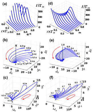
Figure 3: Superradiance (a,d), angular momentum vector $\mathbf{J}$ (b,d) and uncertainty vector $\Delta\mathbf{J}$ (e,f) for fifty identical two-level atoms. (a-c) show the influence of the initial pure states with varying angle $\theta_{i}$ but fixed $\phi_{i}=0$. (d-f) show the influence of increasing mixing (probability $m$) of two pure states with $\left(\theta_{1},\phi_{1}\right)=\left(0,0\right)$ and $\left(\theta_{2},\phi_{2}\right)=\left(\pi/2,0\right)$. $\omega_{c}=\omega_{1}-\omega_{0}=10\pi\Gamma_{10}$ and other parameters are zero. For more details see text.

Fig. 3 (a,b,c) show the results when the initial states are pure states. Fig. 3 (a) shows that the initial radiation rate is finite for $\theta_{i}=\pi$ (the fully excited state), and increases to the maximum for $\theta_{i}=\pi/2$ (the superposition state), and decreases back to zero for $\theta_{i}=0$ (the ground state). The radiation has a pulse structure for $\theta_{i}\in\left(\pi/2,\pi\right]$ and the pulse maximum increases and the pulse center shifts to the earlier time with reducing $\theta_{i}$. In contrast, the radiation shows an exponential decay for $\theta_{i}\in\left(0,\pi/2\right]$ and the time when the radiation vanishes reduces with reducing $\theta_{i}$. Fig. 3 (b) shows that the initial angular momentum $\mathbf{J}$ rotates from the north pole to the equator, and finally to the north pole. In particular, for $\theta_{i}=\pi$ the components $J_{x},J_{y}$ are zero. That is to say, the superradiance from the atoms fully excited is not accompanied by the formation of dipole. Actually, this is the superradiance initially discussed by Dicke (RHDicke, ). However, for $\theta_{i}\neq 0$ the vector $\mathbf{J}$ actually circles around the z-axis before ending up at the south pole. Notice that the components $J_{x},J_{y}$ are not zero. That is to say that for the atoms, which are not fully excited, the superradiance is accompanied by the formation of macroscopic dipole. This corresponds actually to the so-called superfluorescence (JCMacGillivray, ). Fig. 3 (c) shows that the initial uncertainty of angular momentum $\Delta\mathbf{J}$ vector has a fixed length of $\sqrt{N/4}\approx 3.54$ and points to different directions in the plane with $\Delta J_{y}=3.54$ for different $\theta_{i}$. For $\theta_{i}\in\left[\pi/2,\pi\right]$ the length of that vector increases with time and the maximal length reduces with reducing $\theta_{i}$. In contrast, for $\theta_{i}\in\left[0,\pi/2\right]$ the length does not change with time. In all the cases the $\Delta\mathbf{J}$ vector ends at the point $\left(3.54,3.54,0\right)$. In addition, we have also varied the angle $\phi_{i}$ but found no influence on the superradiance.

Fig. 3 (d,e,f) show how the mixed initial states affect the superradiance and the atomic dynamics. In particular, we consider that every single atom is initially in a mixture of the excited state $\left(\theta_{1},\phi_{1}\right)=\left(0,0\right)$ with a probability $m$ and the superposition state $\left(\theta_{2},\phi_{2}\right)=\left(\pi/2,0\right)$ with a probability $1-m$. Fig. 3 (d) shows that the initial radiation rate reduces with increasing $m$ due to the reduced contribution of the superposition state while the radiation maximum increases because of increased contribution of the excited state. Fig. 3 (e) shows that the initial $\mathbf{J}$ vector moves from the equator to the north pole with increasing $m$. $\mathbf{J}$ circles around the z-axis for $m\neq 1$ but shrinks along the $z$-axis for $m=0$. In both cases $\mathbf{J}$ ends eventually at the south pole. Fig. 3 (f) shows that the initial $\Delta\mathbf{J}$ vector goes upwards when $m$ increases from $0$ to $0.5$ but then goes downwards when $m$ further increases to one. The length of the vector increases firstly and then reduces with increasing time. $\Delta\mathbf{J}$ always ends up at the point $\left(3.54,3.54,0\right)$ corresponding to the fully ground state. Notice that the maximal length increases with increasing $m$.

In Appendix A.1 we have further studied how the superradiance and the atomic dynamics are affected by the number of atoms $N$, the frequency detuning $\chi_{10}=\omega_{1}-\omega_{0}-\omega_{c}$, the decay rate $\gamma_{10}$ and the dephasing rate $\xi_{10}$ of individual atoms. We find that the maximum, center, duration of the superradiance pulses change with $N$ according to $N^{2},N^{-1}\mathrm{ln}N,N^{-1}$, respectively. The maximum depends on $\chi_{10}$ according to a Lorentzian shape while the center and duration to a parabolic shape. The maximum changes with $\gamma_{10}$ according to $\exp\left(-\alpha\gamma_{10}\right)$ while the center, duration according to $\left[\gamma_{10}^{2}+\beta\right]^{-2}$ ($\alpha,\beta$ are some constant), respectively.

III.2 Superradiance from Atoms Coherently Driven

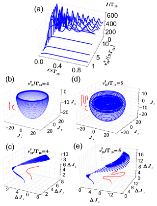
Figure 4: Superradiance (a) and dynamics of angular momentum vector $\mathbf{J}$ (b,d) and its uncertainty $\Delta\mathbf{J}$ (c,e) for fifty identical two-level atoms, which are initially on the ground state and are then driven coherently with a strength $v_{10}^{0}$. (b,c) are results under weak driving $v_{10}^{0}/\left(\pi\Gamma_{10}\right)=4$ while (d,e) under moderate driving $v_{10}^{0}/\left(\pi\Gamma_{10}\right)=5$. We assume that the atoms are resonant to the cavity mode and also to the driving laser, i.e. $\omega_{1}-\omega_{0}=\omega_{d}=\omega_{c}$. We use small transition frequency $\omega_{1}-\omega_{0}=200\times\pi\Gamma_{10}$ to better illustrate the dynamics. The red curves with arrows indicate the direction of the dynamics. Other parameters are zero. For more details see text.

In this subsection, we analyze the superradiance and the dynamics of fifty identical two-level atoms, see Fig. 4, which are driven coherently by an external field with a strength $v_{10}^{0}$ and experience simultaneously a collective decay with the rate $\Gamma_{10}$. If the atoms are only driven coherently, their population follows Rabi oscillation with a period $T=\pi/v_{10}^{0}$. If the atoms experience only the collective decay, their population on the excited state decays in time and the time for vanishing population depends on the number of atoms. For fifty atoms as considered here, we estimate this time as $\tau_{a}=0.2/\Gamma_{10}$.

With the parameters as analyzed above we can now understand the results shown in Fig. 4. For $\tau_{a}/T<1$ or $v_{10}^{0}/\pi<\Gamma_{10}$, the system achieves the steady-state before it starts oscillating because the collective decay is relatively faster than the coherent driving. This leads to the smooth change of the radiation for $v_{10}^{0}/\left(\pi\Gamma_{10}\right)<4$ as shown in Fig. 4 (a), the cup-like trajectory of the vector $\mathbf{J}$ and the hoe-like trajectory of the vector $\Delta\mathbf{J}$ as shown in Fig. 4 (b,c), respectively. Here, the oscillation frequency of $J_{x}$,$J_{y}$ and $\Delta J_{x}$, $\Delta J_{y}$ is determined by the frequency of the external field. By increasing the driving, the ratio $v_{10}^{0}/\left(\pi\Gamma_{10}\right)$ increases. This leads to the increased steady-state radiation, see Fig. 4 (a), and the increased height of the cup-like trajectory of $\mathbf{J}$ as well as the increased length of the hoe-like trajectory of $\Delta\mathbf{J}$ (not shown).

For $\tau_{a}/T=1$, i.e. $v_{10}^{0}/\left(\pi\Gamma_{10}\right)=5$, the two processes are comparable and the system shows oscillations before achieving the steady state, see Fig. 4 (a), which is accompanied by the vase-like trajectory of $\mathbf{J}$ and the tie-like trajectory of $\Delta\mathbf{J}$ as shown in Fig. 4(d,e), respectively. We notice that each oscillation of the radiation is related to one shell of the vase-like trajectory and one fold of the tie-like trajectory. The reduced amplitude of radiation oscillation is related to reduced radius of the shell and of the folded layer. In addition, for $\tau_{a}/T>1$, i.e. $v_{10}^{0}/\left(\pi\Gamma_{10}\right)>5$, the coherent driving is much faster than the collective decay. As a result, we see more oscillations with reduced period before the system achieves the steady-state, see Fig. 4(a), which is accompanied by the spherical lantern-like trajectory of $\mathbf{J}$ and the banana-like trajectory of $\Delta\mathbf{J}$ (not shown), respectively. At this point, we might conclude that the number of turns in the outer shell reduces with increasing driving of the external field.

In Appendix A.2 we have further studied how the superradiance from the atoms driven coherently is influenced by the number of atoms $N$, the frequency detuning $\chi_{10}=\omega_{1}-\omega_{0}-\omega_{c}$ , the decay rate $\gamma_{10}$ and dephasing rate $\xi_{10}$ of individual atoms. We find that with increasing $N$ the superradiance changes from the oscillatory behavior to the steady behavior at long time (due to enhanced collective decay rate). With increasing $\chi_{10}$ the superradiance maximum reduces and the time to achieve steady superradiance reduces (due to off-resonant excitation). With increasing $\gamma_{10},\xi_{10}$, the time to achieve steady radiation reduces and the steady radiation also reduces. In general, $\gamma_{10}$ affects the superradiance much stronger than $\xi_{10}$ since it affects also the population.

III.3 Superradiance from Atoms Pumped Incoherently

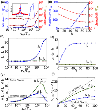
Figure 5: Steady-state spectra, consisting of a sharp peak and a broad background [see inset of (a)], for increasing pumping rate $\gamma_{01}$ (a,b,c, for fifty atoms) and number of atoms $N$ (d,e,f, for fixed pumping rate $\gamma_{01}=20\gamma_{10}$). In (a,d) we show the maximum (blue triangles) and linewidth (red triangles) of the sharp peak (lower triangles) and of the background (upper triangles). In (d) the maximum and the linewidth of the sharp peak (background) are fitted with $-188.05+4.77N$ ($-6.01+0.32N$) and $1.0+18.3\exp\left(-5.7\times 10^{-2}N\right)$ [$10.1+230\exp\left(-4.9\times 10^{-2}N\right)$]. (b-f) show the angular momentum components and their uncertainties: $J_{x}$ and uncertainty $\Delta J_{x}$ (red upper triangles), $J_{y}$ and $\Delta J_{y}$ (green lower triangles), $J_{z}$ and $\Delta J_{z}$ (blue squares). In (c,f) the upper and lower dashed line indicate the limit of the Dicke superradiant states and the atomic product states , respectively. Other parameters are zero. For more details see text.

Steady-state superradiance was firstly studied by D. Meiser and M. J. Holland (DMeiser, ; DMeiser1, ) by solving the superradiance master equation with Monte-Carlo method for tens of atoms (DMeiser1, ) and second-order mean field theory (DMeiser, ) for thousands of atoms. Here, we apply our description to study this phenomenon and unravel more details with exact simulations, see Fig. 5.

Fig. 5 (a,b,c) show the steady-state spectra and the steady-states of fifty identical two-level atoms for increasing pumping rate $\gamma_{01}$. The steady-state spectra consist of not only one sharp peak as discussed in (DMeiser1, ) but also one broad background, see inset of Fig. 5(a). Fitting the spectra with two Lorentzian functions, we have determined the maximum and the linewidth of both the sharp peak and the background, see Fig. 5 (a). In general, the background is about one order of magnitude weaker and broader than the sharp peak. We see that the maximum (blue lines) increases slowly with increasing $\gamma_{01}$ for $\gamma_{01}<\Gamma_{10}$ and then quickly for $\gamma_{01}>\gamma_{c}$, but finally decreases for much larger $\gamma_{01}$. The linewidth (red lines) behaves in opposite to the maximum, which is a reminiscence of Schawlow-Townes relation (SchawlowTownes, ). The smallest linewidth of the sharp peak approaches the collective decay rate $\Gamma_{10}$, which agrees with the results in (DMeiser, ; DMeiser1, ).

We have also computed the total radiation rate $I_{tot}$ and decompose it into the contribution from individual atoms $I_{ind}$ and from the atom-atom correlation $I_{col}$. We find that $I_{tot}$ changes similarly as the spectrum maximum. Importantly, for $\gamma_{01}<\Gamma_{10}$, $I_{col}$ is negative and reduces $I_{tot}$. Thus, we can identify this regime as subradiance regime. For $\gamma_{01}>\Gamma_{10}$, $I_{c}$ is positive and dominates over $I_{ind}$. We can identify this regime as superradiance regime. For $\gamma_{01}\gg\Gamma_{10}$, $I_{col}$ reduces and thus $I_{tot}$ also reduces. This reduction can be attributed to the reduced coupling for higher populated atoms (KDebnath, ). We can identify this regime as the (population) saturation regime (see below).

Fig. 5 (b) shows that the three regimes as identified before are correlated with $J_{z}$ (blue lines), which increases from negative value to positive value (inverted population) and finally saturated value, respectively. Fig. 5 (c) shows a much close correlation with the uncertainties $\Delta J_{x},\Delta J_{y},\Delta J_{z}$. In particular, the uncertainties are smaller than the limit $\sqrt{N/4}=3.5$ (the uncertainty of uncorrelated atoms) for $\gamma_{01}<\Gamma_{10}$, but become larger than that value for $\gamma_{01}>\Gamma_{10}$. In addition, they approach the limit $\sqrt{\left(N/2\right)\left(N/2+1\right)/3}=15.3$ (the uncertainty of correlated atoms in Dicke superradiant states ) for larger $\gamma_{01}$. Notice that $J_{x}$ and $J_{y}$ are always zero and thus there is no macroscopic dipole involved.

Fig. 5 (d-f) show the steady-state spectra and the atomic steady-states for increasing number of atoms $N$. Fig. 5 (d) shows that the maximum of the sharp peak and the background increases quadratically with $N$ for $N<40$ but linearly for $N>40$ while the linewidth reduces exponentially for small $N$ but approaches a constant for large $N$. Fig. 5 (e) shows that the change of the peak maximum is correlated with $J_{z}$, which increases initially but saturates for large $N$. Fig. 5(f) shows that the maximum is more closely correlated with the uncertainty $\Delta J_{l}$. Moreover, we find that $\Delta J_{z}$ departs from the limit $\sqrt{N/4}$ while $\Delta J_{x},\Delta J_{y}$ from $\sqrt{\left(N/2\right)\left(N/2+1\right)/3}$. This indicates that the atoms are between the uncorrelated state and the fully correclated state.

In Appendix A.2, we have further studied how the steady-state spectrum is influenced by the decay rate $\gamma_{10}$ and the dephasing rate $\xi_{10}$ of individual atoms. We find that $\gamma_{10}$ affects the spectrum much stronger than $\xi_{10}$ because $\gamma_{10}$ competes directly with the incoherently pumping $\gamma_{01}$. Increasing $\gamma_{10}$ just tens times, we reduce the spectrum maximum and increase the linewidth by orders of magnitude. In contrast, only by increasing $\xi_{10}$ by one hundred times, we can only reduce the spectrum maximum and linewidth by two or three times. These results suggest that the steady-state superradiance seem to be robust to the dephasing of individual atoms but sensitive to the decay of individual atoms.

IV Conclusions

To sum up, in this article, we presented a collective description of density matrix for identical multi-level atoms. Our description explores symmetry of density matrix in the basis of atomic product states without explicitly applying the symmetry group theory. Since our description removes the redundancy of density matrix elements, it is possible to carry out exact simulation for systems with hundreds of two-level atoms and tens of three- or four-level atoms.

As an example, we applied our description to simulate superradiance from hundreds of two-level atoms, which are either excited initially or driven coherently or pumped incoherently. With the simulation we identified two kinds of superradiance. The first kind does not involve the formation of dipole and appears for the atoms, which are either fully excited initially or pumped incoherently. The second kind does involve the dipole and appears for the atoms, which are initially in superposition states or driven coherently. In addition, we found that the superradiance is more closely correlated with the uncertainties of angular momentum.

In the future, we can apply our description to study superradiance from multi-level atoms (RTSutherland, ). In addition, we can also extend our description in many directions. By extending the description to atoms of multi-species, we can study the cavity-mediated interaction between the species and the resulting effects, such as superradiance beats (MANorcia, ), phase synchronization (MXu-1, ; JMWeiner, ). By including the cavity mode directly rather than eliminating it, we can also develop a description to study the effects in the intermediate or good cavity limit, such as superradiance-to-lasing transition (KDebnath, ; MANorcia-1, ; DATieri, ). By including measurement backactions we can also study the measurement and control of quantum system (HMWiseman, ), e.g. the conditional spin-squeezing (ZChen, ).

Appendix A Supplemental Results

In the main text, we have presented the main results on the superradiance from hundreds of two-level atoms, which are either excited initially or driven coherently or pumped incoherently. In this Appendix, we supplement these results by analyzing the influence of the number of atoms, the decay and dephasing of individual atoms.

A.1 Influence on Superradiance from Atom Initially Excited

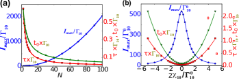
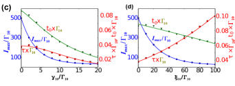
Figure 6: Maximum $I_{max}$ (dots, blue curves), center $t_{0}$ ( triangles, green curves) and duration $\tau$ (squares, red curves) of superradiance pulses for increasing number of atoms $N$ (a), frequency detuning $\chi_{10}=\omega_{1}-\omega_{0}-\omega_{c}$ (b), decay rate $\gamma_{10}$ (c) and dephasing rate $\xi_{10}$ (d). In (b) $\Gamma_{10}^{0}$ is the collective decay rate on resonant condition. In (a,c,d) we focus on the resonant case such that $\Gamma_{10}=\Gamma_{10}^{0}$. In (a) the data are fitted with $I_{max}/\Gamma_{10}=0.54-0.37N+0.21N^{2}$, $t_{0}\Gamma_{10}=\left(0.88/N\right)\ln\left(2.12N\right)$, $\tau\Gamma_{10}=1.88/(0.87+N)$. In (b) the data are fitted with $I_{max}/\Gamma_{10}^{0}=529\left[\left(\alpha-1.38\right){}^{2}+1.\right]^{-1}$, $t_{0}\Gamma_{10}^{0}=0.03-2.18\alpha+0.04\alpha^{2}$, $\tau\Gamma_{10}^{0}=0.08-2.18\alpha+0.08\alpha^{2}$ with $\alpha=2\chi/\Gamma_{10}^{0}$. In (c) the data are fitted with $I_{max}/\Gamma_{10}=33.84+466.99\exp\left(-0.27\beta\right)$, $t_{0}\Gamma_{10}=0.10\times 13.89^{2}\left[\left(\beta+4.89\right)^{2}+14^{2}\right]^{-1}$, $\tau\Gamma_{10}=0.10\times 15.83^{2}\left[\left(\beta+0.26\right)^{2}+16{}^{2}\right]^{-1}$ with the ratio $\beta=\gamma_{10}/\gamma_{c}$. In (d) the data are fitted with $I_{max}/\Gamma_{10}=24+480.5\exp\left(-0.04\delta\right)$, $t_{0}\Gamma_{10}=8.9\times 10^{-2}-2.5\times 10^{-4}\delta$, $\tau\Gamma_{10}=3.7\times 10^{-2}-3.9\times 10^{-4}\delta$ with the ratio $\delta=\xi_{10}/\Gamma_{10}$. Other parameters are zero. For more details see text.

In the following, we discuss the supplemental results on the superradiance from the atoms, which are initially excited. Fig. 6 shows how the maximum $I_{max}$, center $t_{0}$ and duration $\tau$ of the superradiant pulses are affected by the number of atoms $N$ (a), the frequency detuning $\chi_{10}=\omega_{1}-\omega_{0}-\omega_{c}$ (b), the decay rate $\gamma_{10}$ (c) and the dephasing rate $\xi_{10}$ (d). Fig. 6 (a) shows that $I_{max}$ increases as $N^{2}$, while $\tau$ and $t_{0}$ vary according to $1/N$ and $N\ln N$, respectively, which agrees with (LMandel, ) except for small deviation for small $N$. We also observe that $J_{z}$ drops from $N/2$ to $-N/2$ with an accelerated speed for large $N$ and the other components vanish, i.e. $J_{x}=J_{y}=0$ (not shown). In addition, $\Delta J_{z}$, $\Delta J_{x}$, $\Delta J_{y}$ have same structure as the superradiance pulses and their maximum increase with $N$ (not shown).

To better interpret Fig. 6 (b), we introduce the ratio $\alpha=2\chi_{10}/\Gamma_{10}^{0}$ with the collective decay rate $\Gamma_{10}^{0}$ in the resonant case ($\chi_{10}=0$) and express the collective decay $\Gamma_{10}\left(\alpha\right)=\Gamma_{10}^{0}/\left(\alpha^{2}+1\right)$ and the Lamb shift $\Omega_{ll^{\prime}}\left(\alpha\right)=-\Gamma_{10}^{0}\left[\alpha/\left(\alpha^{2}+1\right)\right]$ as functions of this ratio. Fig. 6 (b) shows that $I_{max}$ reduces with increasing $\left|\alpha\right|$ while $t_{0}$ and $\tau$ increases. The relation of $I_{max}$ and $\alpha$ can be fitted with a Lorentzian function, and the relation of $t_{0}$, $\tau$ and $\alpha$ can be well fitted with a parabolic function. We also find that $J_{x}$, $J_{y}$ vanish and $J_{z}$ drops quickly for small $\left|\alpha\right|$ but slowly for large $\left|\alpha\right|$ (not shown). In addition, $\Delta J_{z}$ changes similarly as the radiation.

Fig. 6 (c) shows that $I_{max}$ reduces exponentially with increasing $\beta\equiv\gamma_{10}/\Gamma_{10}$, while $t_{0}$, $\tau$ reduce inversely with the square of $\beta$. We also find that $J_{z}$ follows a $S$-shape for small $\beta$ because of the dominance of $\gamma_{10}$, but decays exponentially for large $\beta$ due to the dominance of $\Gamma_{10}$ (not shown). In addition, $\Delta J_{z}$ follows the change of the superradiance pulses. Fig. 6 (d) shows that $I_{max}$ decreases exponentially, $\tau$ reduces linearly, and $t_{0}$ increases with increasing $\delta=\xi_{10}/\Gamma_{10}$. We also find that $J_{z}$ drops quickly and follows a S-shape for small $\delta$. In addition, $\Delta J_{z}$ follows the change of the superradiance pulses. These results suggest that the decay rate $\gamma_{10}$ affects the superradaince much stronger than the dephasing rate $\xi_{10}$ because it affects directly the population.

A.2 Influence on Superradiance from Atoms Driven Coherently

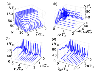
Figure 7: Superradiance for increasing number of atoms $N$ (a), frequency detuning $\chi_{10}=\omega_{1}-\omega_{0}-\omega_{c}$ (b), decay rate $\gamma_{10}$ (c) and dephasing rate $\xi_{10}$ (d). We consider $N=20$ atoms in (b,c,d). The atom-external field coupling is $v_{10}^{0}/\left(\pi\Gamma_{10}\right)=2$. In (b) $\Gamma_{10}^{0}$ is the collective decay rate $\Gamma_{10}$ on resonant condition $\chi_{10}=0$. In (a,c,d) we focus on the resonant condition such that $\Gamma_{10}=\Gamma_{10}^{0}.$ Other parameters are zero. For more details see text.

In the following, we discuss the supplemental results on the superradiance from the atoms, which are driven coherently. Fig. 7 (a) shows that the radiation increases and the number of oscillations reduces when the number of atoms increases to thirty. This is because the time $\tau_{a}$ of the collective decay reduces gradually and becomes comparable with the period $T=\pi/v_{10}^{0}$ of the Rabi oscillations. The radiation becomes constant and the oscillation disappears when the number of atoms exceeds thirty because the time $\tau_{a}$ is smaller than the period $T$. Fig. 7 (b) shows that the maximum and the steady-state value of the radiation $I/\Gamma_{10}$ reduce by fifty percents when the frequency $\omega_{d}$ of the external field is detuned from the atomic transition frequency $\omega_{1}-\omega_{0}$ about sixty times ($\delta=60$) of the collective decay rate.

Fig. 7 (c) shows that the maximum of radiation reduces only a little but the number of oscillations reduces a lot when the individual decay rate increases to ten times ($\beta=10$) of the collective decay rate. The steady-state radiation arrives at the minimum when the two rates are comparable ($\beta=1$) but actually increases a little for large individual decay rate ($\beta>1$). Fig. 7 (d) shows that the individual dephasing rate affects the radiation in a similar way as the individual decay rate. However, the similar effect is achieved when the former rate is about two times of the latter rate, i.e. $\chi\approx 2\beta$.

A.3 Influence on Superradiance from Atoms Incoherently Pumped

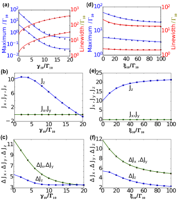
Figure 8: Influence of decay rate $\gamma_{10}$ (a-c) and dephasing rate $\xi_{10}$ (d-f) on the systems with fifty atoms. Shown properties are same as in Fig. 5. In (a) the blue upper and lower triangles are fitted with $0.41+57.82\exp\left(-0.47\alpha\right)$, $58.19\exp\left(-0.43\alpha\right)$ with the ratio $\alpha=\gamma_{10}/\Gamma_{10}$, respectively, and the red upper and lower triangles are fitted with $-38.73+40.57\exp\left(3.07\times 10^{-2}\alpha\right)$, and $-786.49+788.34\exp\left(1.96\times 10^{-2}\alpha\right)$, respectively. In (d) the blue upper and lower triangles are fitted with $21.923+36.3\exp\left(-3.53\times 10^{-2}\beta\right)$, $1.85+3.51\exp\left(-7.52\times 10^{-3}\beta\right)$ with the ratio $\beta=\xi_{10}/\Gamma_{10}$, respectively, and the red upper and lower triangles are fitted with $1.62+0.23\exp\left(-4.49\times 10^{-2}\beta\right)$, $15.81+13.69\exp\left(6.01\times 10^{-2}\beta\right)$, respectively. $\gamma_{01}=20\Gamma_{10}$ and other parameters are zero. For more details see text.

Fig. 8 (a,b,c) show the influence of the individual decay rate $\gamma_{10}$ on systems with fifty atoms. Fig. 8 (a) shows that the maximum of the peak and background reduces with increasing $\gamma_{10}$, while their linewidth behaves oppositely. Fig. 8 (b,c) show that the reduced and broadening spectra are correlated with the reduced $J_{z}$ and uncertainty $\Delta J_{l}$, respectively. Notice that $\Delta J_{x}$ and $\Delta J_{y}$ are initially larger than $\Delta J_{z}$ but approaches it for large $\gamma_{10}$.

Fig. 8 (d,e,f) show the influence of the individual dephasing rate $\xi_{10}$. Fig. 8(d) shows that the steady-state spectrum behaves differently compared to Fig. 8 (a) for $\gamma_{10}$. In this case, the peak linewidth reduces with increasing $\xi_{10}$ while the background linewidth does not change. In addition, the maximum of peak and background do not reduce so strong as the case for $\gamma_{10}$. Fig. 8(e) shows that $J_{z}$ increases first and then saturates with increasing $\xi_{10}$ in contrast to Fig. 8(b) for $\gamma_{10}$. Fig. 8(f) shows that $\Delta J_{l}$ reduce with increasing $\xi_{10}$ in a similar way as Fig. 8 (c) for $\gamma_{10}$ except that $\Delta J_{x}$ and $\Delta J_{y}$ are always larger than $\Delta J_{z}$. However, we should notice that $\xi_{10}$ is in the range $\left[0,100\Gamma_{10}\right]$ while $\gamma_{10}$ is in $\left[0,20\Gamma_{10}\right]$. Thus, $\gamma_{10}$ affects the steady-state superradiance much stronger than $\xi_{10}$. Notice that $\gamma_{10}$ contributes not only to dephasing but also affects the population directly.

Appendix B Angular Moment and Uncertainty

In this appendix, we present the formula to compute the angular moment $\mathbf{J}=\sum_{i=x,y,z}J_{i}\mathbf{e}_{i}$ and its uncertainty $\Delta\mathbf{J}=\sum_{i=x,y,z}\Delta J_{i}\mathbf{e}_{i}$. The components $J_{x}$ and $J_{y}$ are expectation value of the angular momentum operators $\sigma_{x}=\left(1/2\right)\left(\sigma_{+}+\sigma_{-}\right)$, $\sigma_{y}=-\left(i/2\right)\left(\sigma_{+}-\sigma_{-}\right)$. Thus, they can be calculated as $J_{x}=\left(1/2\right)\left(C_{10}+C_{01}\right)$ and $J_{y}=-\left(i/2\right)\left(C_{10}-C_{01}\right)$ with the expectation value of the collective creation $\sigma^{+}$ and annihilation operator $\sigma^{-}$: $C_{10}\equiv\left\langle\sigma^{+}\right\rangle=\sum_{l=0}^{N}C_{N}^{l}\left(N-l\right)\left\langle l,1,0,N-l-1\right\rangle,$$C_{01}\equiv\left\langle\sigma^{-}\right\rangle=\sum_{l=0}^{N}C_{N}^{l}l\left\langle l-1,0,1,N-l\right\rangle$. On the right side, the numbers from the left to right are $n_{11},n_{10},n_{01},n_{00}$. The component $J_{z}\equiv\left(1/2\right)\left\langle\sigma_{z}\right\rangle$ can be calculated with the expectation value $\left\langle\sigma_{z}\right\rangle$ of the collective Pauli operator $\sigma_{z}=\sigma_{11}-\sigma_{00}$. In return, this expectation value $\left\langle\sigma_{z}\right\rangle=P_{1}-P_{0}$ can be computed with the population of the upper level $P_{1}\equiv\left\langle\sigma_{11}\right\rangle$ and lower level $P_{0}\equiv\left\langle\sigma_{00}\right\rangle$, respectively: $P_{1}=\sum_{l=0}^{N}C_{N}^{l}l\left\langle l,0,0,N-l\right\rangle,$$P_{0}=\sum_{l=0}^{N}C_{N}^{l}\left(N-l\right)\left\langle l,0,0,N-l\right\rangle.$ The components $\Delta J_{i}$ of the uncertainty vector $\Delta\mathbf{J}$ can be calculated with $\Delta J_{i}=\sqrt{\left\langle j_{i}^{2}\right\rangle-J_{i}^{2}}$. We can evaluate the expectation value of the square of the angular momentum operators:

$$\left\langle j_{x}^{2}\right\rangle=\left(1/4\right)\sum_{l=0}^{N}C_{N}^{l}[l\left(l-1\right)\left\langle l-2,0,2,N-1\right\rangle$$

$$+N\left\langle l,0,0,N-l\right\rangle+2l\left(N-l\right)\left\langle l-1,1,1,N-l-1\right\rangle$$

$$+\left(N-l\right)\left(N-l-1\right)\left\langle l,2,0,N-l-2\right\rangle],$$ (26)

$$\left\langle j_{y}^{2}\right\rangle=\left(-1/4\right)\sum_{l=0}^{N}C_{N}^{l}[l\left(l-1\right)\left\langle l-2,0,2,N-l\right\rangle$$

$$-N\left\langle l,0,0,N-l\right\rangle-2l\left(N-l\right)\left\langle l-1,1,1,N-l-1\right\rangle$$

$$+\left(N-l\right)\left(N-l-1\right)\left\langle l,2,0,N-l-2\right\rangle],$$ (27)

$$\left\langle j_{z}^{2}\right\rangle=\left(1/4\right)\sum_{l=0}^{N}C_{N}^{l}\left(2l-N\right)^{2}\left\langle l,0,0,N-l\right\rangle.$$ (28)

References

- (1) R. H. Dicke, Coherence in Spontaneous Radiation Processes, Phys. Rev. 93, 1 (1954)
- (2) A. V. Andreev, V. I. Emel’yanov, and Y. A. II’inskii, Collective Spontaneous Emission (Dicke Superradiance) Usp. Fiz, Nauk 131, 653-694, (1980)
- (3) Barry M. Garraway, The Dicke model in Quantum Optics: Dicke Model Revisited, Phil. Trans. R. Soc. A 369, 1137-1155 (2011)
- (4) R. Bonifacio and P. Schwendimann, F. Haake, Quantum Statistical Theory of Superradiance, Phys. Rev. A 4, 302 (1970)
- (5) A. V. Andreev, Theory of Cooperative Spontaneous Emission, Sov. J. Quantum Electron 8, 476 (1978)
- (6) C. T. Lee, Exact Solution of the Superradiance Master Equation. I Complete Initial Excitation, Phys. Rev. A, 15, 2019 (1977)
- (7) L. M. Narducci, C. M. Bowden, Exact Diffusion Equation for a Model for Superradiant Emission, Phys. Rev. A 9, 829 (1974)
- (8) R. J. Glauber, F. Hakke, Superradiant Pulses and Directed Angular Momentum States, Phys. Rev. A. 13, 357 (1976)
- (9) D. Meiser, J. Ye, D. R. Carlson, and M. J. Holland, Prospects for a Millihertz-Linewidth Laser, Phys. Rev. Lett. 102, 163601 (2009)
- (10) D. Meiser, M. J. Holland, Steady-State Superradiance with Alkaline-Earth-Metal Atoms, Phys. Rev. A 81, 033847 (2010)
- (11) B. A. Chase, J. M. Geremia, Collective Processes of an Ensemble of Spin-1/2 Particles, Phys. Rev. A 78, 052101 (2008)
- (12) B. Q. Baragiola, B. A. Chase and J. M. Geremia, Collective Uncertainty in Partially Polarized and Partially Decohered Spin-1/2 Systems, Phys. Rev. A 82, 032104 (2010)
- (13) F. Damanet, D. Braun, J. Martin, Cooperative Spontaneous Emission from Indistinguishable Atoms in Arbitrary Motional Quantum States, Phys. Rev. A 94, 033838 (2016)
- (14) N. Shammah, S. Ahmed, N. Lambert, S. De Liberato, and F. Nori, Open Quantum Systems with Local and Collective Incoherent Processes: Efficient Numerical Simulations Using Permutational Invariance, Phys. Rev. A 98, 063815 (2018)
- (15) M. Richter, M. Gegg, T. S. Theuerholz, A. Knorr, Numerically Exact Solution of the Many Atom-cavity Laser Problem: Application to the Fully Quantized Spaser Emission, Phys. Rev. B 91, 035306 (2015)
- (16) U. Martini, Cavity QED with Many Atoms, PhD Dissertation, Ludwig-Maximilians-Universität München
- (17) M. Gegg, M. Ricther, Efficient and Exact Numerical Approach for Many Multi-level Systems in Open System CQED, New J. Phys. 18, 043037 (2016)
- (18) Y. Zhang, V. May, Theory of Molecule Metal Nano-particle Interaction: Quantum Description of Plasmonic Lasing, J. Chem. Phys. 142, 224702 (2015)
- (19) P. Kirton, J. Keeling, Suppressing and Restoring the Dicke Superradiance Transition by Dephasing and Decay, Phys. Rev. Lett. 118, 123602 (2017)
- (20) M. Xu, D. A. Tieri, and M. J. Holland, Simulating Open Quantum System by Applying SU(4) to Quantum Master Equations, Phys. Rev. A 87, 062101 (2013)
- (21) P. Meystre, M. Sargent, Elements of Quantum Optics (Springer- Verlag, Berlin, 1990)
- (22) L. Mandel, E. Wolf, Optical Coherence and Quantum Optics, Cambridge University Press, 1995
- (23) J. C. MacGillivray and M. S. Feld, Theory of Superradiance in an Extended Optically Thick Medium, Phys. Rev. A. 14, 1169 (1976)
- (24) J. Ma, X. Wang, C. P. Sun and F. Nori, Quantum Spin Squeezing, Phys. Rep. 509, 89 (2011)
- (25) A. L. Schawlow and C. H. Townes, Infrared and Optical Masers, Phys. Rev. 112 (6), 1940 (1958)
- (26) K. Debnath, Y. Zhang and K. Mølmer, Lasing in the Superradiant Crossover Regime, Phys. Rev. A 98, 063837 (2018)
- (27) R. T. Sutherland and F. Robicheaux, Superradiance in Inverted Multilevel Atomic Clouds, Phys. Rev. A 95, 033839 (2017)
- (28) M. A. Norcia, M. N. Winchester, J. R. K. Cline, J. K. Thompson, Superradiance on the Millihertz Linewidth Strontium Clock Transition Sci. Adv. 2, e1601231 (2016)
- (29) M. Xu, D. A. Tieri, E. C. Fine, J. K. Thompson, and M. J. Holland, Synchronization of Two Ensembles of Atoms, Phys. Rev. Lett. 113, 154101 (2014)
- (30) J. M. Weiner, K. C. Cox, J. G. Bohnet, and J. K. Thompson, Phase Synchronization inside a Superradiant Laser, Phys. Rev. A 95, 033808 (2017)
- (31) M.A. Norcia, J.K. Thompson, Cold-Strontium Laser in the Superradiant Crossover Regime, Phys. Rev. X 6, 011025 (2016)
- (32) D. A. Tieri, M. Xu, D. Meiser, J. Cooper, M. J. Holland, Theory of the Crossover from Lasing to Steady State Superradiance, arXiv:1702.04830 (2017)
- (33) H. M. Wiseman and G. J. Milburn, Quantum Measurement and Control (Cambridge University Press, UK, 2010)
- (34) Z. Chen, J. G. Bohnet, S. R. Sankar, J. Dai, and J. K. Thompson, Conditional Spin Squeezing of a Large Ensemble via the Vacuum Rabi Splitting, Phys. Rev. Lett. 106, 133601 (2011)