Spinor fields in spherical symmetry.
Einstein-Dirac and other space-times

K.A. Bronnikov,^a,b,c,1 Yu.P. Rybakov,^b,2 and Bijan Saha^b,d,3
a   Center for Gravitation and Fundamental Metrology, VNIIMS, 46 Ozyornaya St., Moscow 119361, Russia;
^b   Peoples’ Friendship University of Russia (RUDN University), ul. Miklukho-Maklaya 6., Moscow 117198, Russia;
^c   National Research Nuclear University “MEPhI” (Moscow Engineering Physics Institute), Moscow, Russia;
^d  Laboratory of Information Technologies, Joint Institute for Nuclear Research, Dubna
          141980 Dubna, Moscow region, Russia

We discuss the static, spherically symmetric Einstein-spinor field system in the possible presence of various spinor field nonlinearities. We take into account that the spinor field energy-momentum tensor (EMT) has in general some off-diagonal components, whose vanishing due to the Einstein equations substantially affects the form of the spinor field itself and the space-time geometry. In particular, the EMT structure with any spinor field nonlinearities turns out to be the same as that of the EMT of a minimally coupled scalar field with a self-interaction potential. Therefore many results previously obtained for systems with such scalar fields are directly extended to the Einstein-spinor field system. Some special solutions are obtained and discussed, in particular, a solution for the Einstein-Dirac system (which lack asymptotic flatness) and some examples with spinor field nonlinearities.

1 Introduction

In the recent past, the spinor description of matter and dark energy was used to draw a picture of the Universe evolution within the scope of Bianchi-type anisotropic cosmological models [1, 2, 3, 4]. It was found that the approach in question gives rise to a variety of solutions depending on the choice of the spinor field nonlinearity. Owing to its sensitivity to the gravitational field, the spinor field brings some unexpected features to the behavior of the gravitational fields and cosmological models. Bearing this in mind, in this paper we consider nonlinear spinor fields coupled to spherically symmetric gravitational fields. Since a variety of astrophysical systems such as stars and black holes are fairly well described within spherical symmetry, the use of spinor fields in this area might be very promising.

The existence of off-diagonal components of the energy-momentum tensor (EMT) of the spinor field even in the simplest cases together with the Fierz identities relating different invariants composed from the bilinear forms of the spinor field impose restrictions either on the geometry of space-time or on the behavior of the spinor field itself or on both of them. As a result, the spinor approach gives rise to a variety of interesting solutions depending on the choice of a spinor field nonlinearity. In particular, in cosmology this approach allows us to explain the late-time acceleration of the Universe expansion, generates regular solutions and causes rapid isotropization of the initially anisotropic Universe. Moreover, the spinor field nonlinearity can simulate different types of fluids and some possible kinds of dark energy [1, 2, 3, 4]. This success of the spinor approach in cosmology leads many authors to consider it in astrophysics and other areas as well. For example, a non-Abelian SU(2) Proca field interacting with nonlinear scalar and spinor fields were studied in [5]. Scattering of a Dirac spinor particle in the field of a Schwarzschild black hole was studied in[6]. The Dirac equation in curved 5D spherically symmetric space-time was studied in [7]. A nonlinear spinor field minimally coupled to Maxwell and Proca fields have been considered in a spherically symmetric space-time [8].

In a recent paper [9], a nonlinear spinor field in spherically symmetric space-times was studied, and it was shown that the existence of nontrivial EMT components imposes substantial restrictions on both the spinor field and the geometry. In the present paper, we make some further observations on the properties of the Einstein-spinor field system in static, spherically symmetric space-times and discuss some exact solutions. It turns out, in particular, that the EMT of a spherically symmetric spinor field, after eliminating its possible off-diagonal components, has the same structure as that of a static scalar field, and therefore a number of results known for the Einstein-scalar field system, concerning the possible existence of Killing horizons and wormholes, are directly extended to the Einstein-spinor system. Next, we discuss exact solutions with the Dirac linear spinor field and some kinds of spinor field nonlinearities.

2 The Einstein-spinor equations

2.1 General equations

Let us consider a system of (in general, nonlinear) spinor and gravitational fields in the framework of general relativity. The action can be written in the form

$${\cal S}(g;\psi,\bar{\psi})=\int\,\sqrt{-g}d^{4}x\left(\frac{R}{2\varkappa}+L_{\rm sp}\right),$$ (1)

where $R$ is the scalar curvature, $\varkappa=8\pi G$, $G$ being the Newtonian gravitational constant, and $L_{\rm sp}$ is the spinor field Lagrangian which we take in the form

$$L_{\rm sp}=\frac{\imath}{2}\left[\bar{\psi}\gamma^{\mu}\nabla_{\mu}\psi-\nabla_{\mu}\bar{\psi}\gamma^{\mu}\psi\right]-m\bar{\psi}\psi-F,$$ (2)

with the spinor field mass $m$ and the nonlinear term $F=F(K)$, where $K$ is one of the four expressions $\{I,\,J,\,I+J,\,I-J\}$, and we use the following notations:

$$I=S^{2},\quad\ J=P^{2};\hskip 28.45274ptS=\bar{\psi}\psi,\quad\ P=i\bar{\psi}\gamma^{5}\psi.$$ (3)

The spinor field equations corresponding to the Lagrangian (2) are

$$\imath\gamma^{\mu}\nabla_{\mu}\psi-m\psi-{\cal D}\psi-\imath{\cal G}\gamma^{5}\psi = 0,$$ (4a)

$$\imath\nabla_{\mu}\bar{\psi}\gamma^{\mu}+m\bar{\psi}+{\cal D}\bar{\psi}+\imath{\cal G}\bar{\psi}\gamma^{5} = 0,$$ (4b)

where $\nabla_{\mu}\psi=\partial_{\mu}\psi-\Gamma_{\mu}\psi$ and $\nabla_{\mu}\bar{\psi}=\partial_{\mu}\bar{\psi}+\bar{\psi}\Gamma_{\mu}$, the matrices $\Gamma_{\mu}$ being those of the spinor affine connection. Furthermore, we denote ${\cal D}=2SF_{K}K_{I}$ and ${\cal G}=2PF_{K}K_{J}$, with $F_{K}=dF/dK$, $K_{I}=dK/dI$ and $K_{J}=dK/dJ$. Using Eqs. (4), it can be shown that

$$L_{\rm sp}=2KF_{K}-F.$$ (5)

The stress-energy tensor (SET) of the spinor field is given by

$$T_{\mu}^{\nu}=\frac{\imath}{4}g^{\rho\nu}\left(\bar{\psi}\gamma_{\mu}\nabla_{\rho}\psi+\bar{\psi}\gamma_{\rho}\nabla_{\mu}\psi-\nabla_{\mu}\bar{\psi}\gamma_{\rho}\psi-\nabla_{\rho}\bar{\psi}\gamma_{\mu}\psi\right)-\delta_{\mu}^{\nu}L_{\rm sp}.$$ (6)

2.2 Static spherical symmetry

In what follows we consider the general static, spherically symmetric metric

$$ds^{2}=e^{2\gamma}dt^{2}-e^{2\alpha}du^{2}-e^{2\beta}(d\theta^{2}+\sin^{2}\theta\,d\varphi^{2})$$ (7)

where $\alpha,\beta,\gamma$ are functions of an arbitrarily chosen radial coordinate $u$. The SET $T_{\mu}^{\nu}$ of the spinor field then has, in general, the following nonzero components [9]:

$$T^{0}_{0} = T_{2}^{2}=T_{3}^{3}=F-2KF_{K},$$ (8a)

$${}T^{1}_{1} = mS+F,$$ (8b)

$$T^{0}_{1} = \frac{1}{4}\cot\theta\,e^{\alpha-\gamma-\beta}A^{3},$$ (8c)

$$T^{0}_{2} = -\frac{1}{4}(\gamma^{\prime}-\beta^{\prime})\,e^{\beta-\alpha-\gamma}A^{3},$$ (8d)

$$T^{0}_{3} = \frac{1}{4}(\gamma^{\prime}-\beta^{\prime})\,e^{\beta-\alpha-\gamma}\sin\theta A^{2}+\frac{1}{4}e^{-\gamma}\cos\theta A^{1}.$$ (8e)

where the prime stands for $d/du$, and $A^{\mu}$ are components of the pseudovector $A^{\mu}=\bar{\psi}\gamma^{5}\gamma^{\mu}\psi$. Since the Einstein tensor $G_{\mu}^{\nu}$ for the metric (7) is diagonal, due to the Einstein equations we must have the off-diagonal components $T^{0}_{i}=0$, whence

$$A^{3}=0,\hskip 28.45274ptA^{1}=A^{2}(\beta^{\prime}-\gamma^{\prime})e^{\beta-\alpha}\tan\theta.$$ (9)

These relations impose certain constraints on the components of the spinor field but do not restrict the very existence of solutions to the spinor equations and do not directly affect the form of the Einstein equations, see more details in [9].

It should also be noted that the expressions for $T^{0}_{i}$ do not depend on the spinor field nonlinearity.

With (8) and (9), the nontrivial components of the Einstein equations can be written as

$$\gamma^{\prime\prime}+\gamma^{\prime}(-\alpha^{\prime}+2\beta^{\prime}+\gamma^{\prime}) = \varkappa e^{2\alpha}(-F+KF_{K}-mS/2),$$ (10a)

$${}e^{2(\alpha-\beta)}-2\beta^{\prime}\gamma^{\prime}-\beta^{\prime}{}^{2} = \varkappa e^{2\alpha}(mS+F),$$ (10b)

$${}-e^{2(\alpha-\beta)}+\beta^{\prime\prime}+\beta^{\prime}(-\alpha^{\prime}+2\beta^{\prime}+\gamma^{\prime}) = \varkappa e^{2\alpha}(-F+KF_{K}-mS/2),$$ (10c)

where the first-order equation (10b) is $G^{1}_{1}=-\varkappa T^{1}_{1}$ while the other two are components of the equations $R_{\mu}^{\nu}=-\varkappa(T_{\mu}^{\nu}-{{\textstyle\frac{1}{2}}}\delta_{\mu}^{\nu}T)$. The conservation law $\nabla_{\nu}T_{\mu}^{\nu}=0$ leads to

$$(mS+F)^{\prime}+(\gamma^{\prime}+2\beta^{\prime})(mS+2KF_{K})=0.$$ (11)

One can notice that due to Eqs. (10) the opportunity $\beta^{\prime}-\gamma^{\prime}=0$ (hence $A^{1}=0$) that could be significant in (9), should be discarded since in this case the difference of (10a) and (10c) leads to the impossible equality $e^{2\alpha-2\beta}=0$.

Let us now consider two different choices of the nature of the spinor field. First, suppose $K=I=S^{2}$, then, since $F^{\prime}=2SF_{K}S^{\prime}$, from (11) we find (provided that $m+2SF_{K}\neq 0$)

$$S=S_{1}e^{-(\gamma+2\beta)},\qquad S_{1}={\rm const}>0.$$ (12)

We take $S_{1}>0$ since the quantity $S={\overline{\psi}}\psi$ is positive-definite.

Second, suppose that $K$ is any of the variants $\{I,\,J,\,I+J,\,I-J\}$, and consider a massless spinor field ($m=0$), as was done in cosmology [1, 2]. Then, assuming $F(K)\neq{\rm const}$, Eq. (11) leads to

$$K=K_{1}e^{-2(\gamma+2\beta)},\qquad K_{1}={\rm const}.$$ (13)

Evidently, the case $m=0,\ K=I=S^{2}$ belongs to both two variants, and then $K_{1}=S_{1}^{2}$.

Equations (8)–(13) immediately lead to a number of important consequences.

1. By (8a), we have $T^{0}_{0}=T_{2}^{2}=T_{3}^{3}$. This property is the same as is known for minimally coupled scalar fields with arbitrary self-interaction potentials, and this immediately leads to the same conclusion as was proved in [10] on the basis of this equality, concerning the possible global structure of any space-time whose metric is obtained with this SET. According to the global structure theorem from [10],

There can be at most two horizons at which $e^{\gamma}=0$. Around a static region, horizons can only be simple (non-extremal).

In particular, if there is a static spatial infinity (be it flat, AdS or any other), there can be only one simple horizon, similar to that in a Schwarzschild  black hole.

2. In the case of a linear spinor field when $F=0$, we have $T^{0}_{0}=T_{2}^{2}=T_{3}^{3}=0$, and the only nontrivial SET component is $T_{1}^{1}=mS$ which is nonzero only for a massive spinor field. A massless (neutrino) field is “stealth” in the sense that its SET is completely zero.

Furthermore, a space-time with $T_{1}^{1}=mS$ cannot be asymptotically flat. Indeed, asymptotic flatness requires that at large $r\equiv e^{\beta}$ the metric should be approximately Schwarzschild, that is,

$$e^{2\gamma}=1-2M/r+O(r^{-2}),\hskip 28.45274pte^{2\alpha}=1+2M/r+O(r^{-2}),$$

from which it follows that all $G_{\mu}^{\nu}=O(r^{-4})$, and by the Einstein equations the same is required for $T_{\mu}^{\nu}$, whereas by (12) $T_{1}^{1}=O(r^{-2})$.

This conclusion is also true with any nonlinearity $F(I)$, except for the special case where this nonlinearity behaves precisely as $-mS$ at small $S$ and thus exactly eliminates the mass term $mS$ in $T^{1}_{1}$; the other SET components then also behave as $o(S)$ at small $S$.

If $m=0$, then, according to (12) and (13), the space-time can be asymptotically flat if $F(K)\sim K$ or $F(K)=o(K)$ at small $K$.

3. A necessary condition for the existence of wormhole throats is that $T^{0}_{0}-T^{1}_{1}<0$, which violates the Null Energy Condition. With the tensor (8) this inequality reads

$$-mS-2KF_{K}<0.$$ (14)

The inequality (14) holds both for a linear massive field with $m>0$ and any nonlinearities such that $KF_{K}>0$.

3 Einstein-Dirac solutions

Let us consider a linear Dirac spinor field, in which case the only nonzero component of the energy-momentum tensor (EMT) $T_{\mu}^{\nu}$ is $T^{1}_{1}=mS(x)$, and the conservation law implies $S(x)\sim e^{-(2\beta+\gamma)}$ (see Eq. (12)).

Let us choose the curvature radial coordinate $u=r$ in the metric (7) (so that $e^{\beta}=r$), Then, in the general case, the temporal component of the Einstein equations can be presented in the integral form:

$$e^{-2\alpha}=1-\frac{\varkappa}{r}\int T^{0}_{0}r^{2}dr-\frac{1}{3}\Lambda r^{2},$$ (15)

where $\Lambda$ is the cosmological constant included in this case for generality. With $T^{0}_{0}=0$, it follows, in full similarity with the Schwarzschild-de Sitter solution,

$$e^{-2\alpha}=1-\frac{2M}{r}-\frac{1}{3}\Lambda r^{2},\qquad M={\rm const}.$$ (16)

Let us substitute it into the ${1\choose 1}$ component of the Einstein equations, having the form

$$e^{-2\alpha}\bigg{(}\frac{2\gamma^{\prime}}{r}+\frac{1}{r^{2}}\bigg{)}-\frac{1}{r^{2}}+\Lambda=-\varkappa mS.$$ (17)

With (12) we obtain

$$1+2r\gamma^{\prime}+(\Lambda r^{2}-1)e^{2\alpha}+S_{2}e^{2\alpha-\gamma}=0,$$ (18)

where $\alpha(r)$ should be substituted from (16) and $S_{2}=\varkappa mS_{1}>0$. Equation (18) is a linear first-order equation with respect to $y(r)=e^{\gamma}$:

$$2ry^{\prime}+\big{[}1+(\Lambda r^{2}-1)e^{2\alpha}\big{]}y=-S_{2}e^{2\alpha}.$$ (19)

In the general case $\Lambda\neq 0$, $M\neq 0$ its solution can be found in quadratures by standard methods, but here we will restrict ourselves to simplest special cases.

1. $M=\Lambda=0$. Then from (19) it follows

$$e^{\gamma}={{\displaystyle\frac{1}{2}}}S_{2}\ln\frac{r_{0}}{r},\hskip 28.45274ptr_{0}={\rm const}>0,$$ (20)

and the range of $r$ is $0<r<r_{0}$. The metric has the form

$$ds^{2}=\frac{1}{4}S_{2}^{2}\Big{(}\ln\frac{r_{0}}{r}\Big{)}^{2}dt^{2}-dr^{2}-r^{2}d\Omega^{2}.$$ (21)

As $r\to 0$ we have $e^{\gamma}\to\infty$, a repulsive singularity. At $r=r_{0}$, on the contrary, $e^{\gamma}\to 0$, it is an attracting singularity.

2. $M=0,\ \Lambda\neq 0$. Then Eq. (19) is solved to give

$$e^{\gamma}=\frac{S_{2}}{2}\bigg{[}-1+\frac{\sqrt{b^{2}-\eta r^{2}}}{b}\ln\frac{C(b+\sqrt{b^{2}-\eta r^{2}})}{r}\biggr{]}=\frac{S_{2}}{2}\bigg{[}-1+\sqrt{1-\eta z^{2}}\ln\Big{(}C\frac{1+\sqrt{1-\eta z^{2}}}{z}\Big{)}\bigg{]},$$ (22)

where $C>0$ is an integration constant, and we are using the notations

$$b=\sqrt{|\Lambda/3|},\qquad\eta=\mathop{\rm sign}\nolimits\Lambda,\qquad z=r/b.$$

It is easy to verify that at $r=0$ in all cases we have a repulsive singularity due to $e^{\gamma}\to\infty$. However, other properties of the metric crucially depend on the sign of $\Lambda$.

If $\Lambda>0$, that is, $\eta=1$, the solution is defined in the range $0<z<z_{0}<1$, or equivalently $0<r<r_{0}<b$ (where $r_{0}=bz_{0}$), in which the quantity $y(r)=e^{\gamma(r)}$ is positive. By definition $r_{0}$ is the value of $r$ at which $y=0$, and since $y^{\prime}(r_{0})$ is finite, the derivative $\gamma^{\prime}(r)=y^{\prime}/y$ is infinite at $r=r_{0}$, which leads to a curvature singularity. Thus the solution exists between two singularities and does not reach the value $r=b$ at which $e^{2\alpha}$ would change its sign similarly to the de Sitter metric. The value of $z_{0}=r_{0}/b$ does not depend on $b$ but depends on $C$ as shown in Fig. 1a.

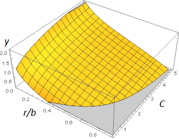
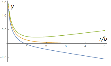
a                                                                  b

Figure 1: Solutions $y(r)=e^{\gamma}$ to Eq. (19) for $M=0$: a — 3D plot for $\Lambda>0$, $S_{2}=1$; b — plots for $\Lambda<0$, $S_{2}=1$ and $C=0.8,\ 1,\ 1.2$ (bottom-up).

If $\Lambda<0$, that is, $\eta=-1$, the function $e^{-2\alpha}=1+r^{2}/b^{2}$ is the same as in the AdS metric and is positive at all $r>0$, but $e^{\gamma}$ is quite different from its AdS counterpart, its behavior depending on the constant $C$. More specifically, if $C<1$, $e^{\gamma}$ turns to zero at some finite $r=r_{0}$ and leads to a singularity in the same way as in the case $\Lambda>0$. If $C=1$, then $e^{\gamma}$ remains positive at all $r$ but vanishes as $r\to\infty$. Lastly, if $C>1$, the solution is also defined ar all $r>0$, and at large $z$ there is a linear asymptotic growth, $e^{\gamma}\approx r(S_{2}/2)\ln C$, so that $e^{2\gamma}\sim r^{2}$ as in the AdS metric, but in general the AdS relation $\alpha+\gamma=0$ does not hold even asymptotically.

3. $\Lambda=0,\ M\neq 0$. Then we can rewrite Eq. (19) in the form

$$2r(r-2M)y^{\prime}-2My+rS_{2}=0,$$ (23)

and its solution is

$$y(r)\equiv e^{\gamma}=+S_{2}\bigg{[}1-\frac{\sqrt{r-2M}}{\sqrt{r}}\ln\frac{\sqrt{r}+\sqrt{r-2M}}{C_{1}}\bigg{]},\qquad C_{1}={\rm const}>0.$$ (24)

Note that $M$ is here, in general, not a mass, and there is no reason to assume its particular sign.

In all cases there is a value $r_{0}$ of the radial coordinate such that $e^{\gamma}(r_{0})=y(r_{0})=0$ but $y^{\prime}(r_{0})\neq 0$. It is a singularity (see footnote 1) that separates two ranges of $r$. The range $r>r_{0}$ extends to infinity with the asymptotic behavior $e^{\gamma}\sim\ln(r/r_{0})$.

If $M>0$, the two ranges are $2M<r<r_{0}$ and $r>r_{0}$. It is of interest that the algebraic curvature invariants are finite at $r=2M$ but the solution cannot be extended beyond this value of $r$ due to loss of analyticity.

If $M<0$, the two ranges are $0<r<r_{0}$ and $r>r_{0}$, and the center $r=0$.is a repulsive singularity.

4 Some solutions with nonlinear spinor fields

In this section we will describe some solvable examples with massless ($m=0$) nonlinear spinor fields.

1. Consider first the case of a linear dependence of $F$ on any of the spinor invariants $K$, that is, $F=\lambda K$, $\lambda={\rm const}$. In this case the SET has the form

$$T_{\mu}^{\nu}=-\lambda K\mathop{\rm diag}\nolimits(1,-1,1,1),$$ (25)

whose structure coincides with that known for a massless, minimally coupled scalar field, which is canonical if $\lambda K<0$ and phantom if $\lambda K>0$. Consequently, the Einstein equations lead to the same metrics, the Fisher and anti-Fisher ones for the canonical and phantom fields, respectively. A brief unified presentation of these metrics involving their all four branches uses the harmonic radial coordinate $u$ defined by the coordinate condition $\alpha=2\beta+\gamma$ [12]:

$${}ds^{2}=e^{-2hu}dt^{2}-\frac{e^{2hu}}{s^{2}(k,u)}\bigg{[}\frac{du^{2}}{s^{2}(k,u)}+d\Omega^{2}\bigg{]},$$

$${}s(k,u):=\left\{\begin{array}[]{ll}k^{-1}\sinh ku,&k>0\\ u,&k=0\\ k^{-1}\sin ku,&k<0,\end{array}\right.$$ (29)

where the constants $h$ and $k$ are also involved in the relation that follows from Eq. EE11 with (13)

$$k^{2}\mathop{\rm sign}\nolimits k=h^{2}-\varkappa\lambda K_{1}.$$ (30)

If $\lambda K_{1}<0$, we have $k>0$, we are dealing with Fisher’s metric (4), in which $u\in{\mathbb{R}}_{+}$, the value $u=0$ corresponds to spatial infinity where the metric is asymptotically flat, and the Schwarzschild mass $M$ is equal to $h$. As $u\to\infty$, there is a naked, attracting (if $M>0$) singularity with $g_{tt}=e^{2\gamma}\to 0$.

If $\lambda K_{1}>0$, the constant $k$ may be zero, positive or negative, and accordingly the metric (4) (often called the anti-Fisher metric) splits into three branches. In all of them the metric is asymptotically flat (again at $u=0$ with the Schwarzschild mass $M=h$), but now there is no center (the radius $r=e^{\beta}$ never turns to zero), instead, there are throats (i.e., regular minima of the function $r(u)$), and the branch $k<0$ describes twice asymptotically flat wormholes. The second spatial infinity corresponds to $u=\pi/|k|$. The (anti-)Fisher metrics have been described and discussed in detail in many papers, we will not do it here and refer the reader to the papers [11, 12, 13, 18] and references therein.

According to the definitions of the invariants $I,J,K$ (see (3)), both $I$ and $J$ are positive-definite, therefore, if $K$ equals $I$, $J$ or $I+J$, the sign of the energy density $T^{0}_{0}$ in (25) (in other words, the canonical or phantom nature of the nonlinear spinor field) is determined by the coupling constant $\lambda$, and only if $K=I-J$, this sign is determined by that of the combination $\lambda K_{1}$.

2. In the general case, due to the equality $T^{0}_{0}=T^{2}_{2}\ \Rightarrow\ R^{0}_{0}=R^{2}_{2}$, the corresponding combination of the Einstein equations admits integration in terms of the quasiglobal coordinate $x$ defined by the condition $\alpha+\gamma=0$. Denoting $e^{2\gamma}=A(x)$ and $e^{\beta}=r$, we write the metric in the form

$$ds^{2}=A(x)dt^{2}-\frac{dx^{2}}{A(x)}-r^{2}(x)d\Omega^{2}.$$ (31)

The equation $R^{0}_{0}=R^{2}_{2}$ then reads

$$A(r^{2})^{\prime\prime}-A^{\prime\prime}r^{2}=2$$ (32)

(the prime denotes $d/dx$) and is easily integrated giving

$$\bigg{(}\frac{A}{r^{2}}\bigg{)}^{\prime}=\frac{6M-2x}{r^{4}},\hskip 28.45274ptA(x)=r^{2}\int\frac{6M-2x}{r^{4}}dx,\hskip 28.45274ptM={\rm const},$$ (33)

which yields $A(x)$ if $r(x)$ is known.

Equation (33) thus makes it possible to find solutions to our problem using the inverse problem method: given $r(x)$ in a form of interest for some reasons, from (33) we find $A(x)$, so that the metric is known completely, and the spinor filed nonlinearity for which it is a solution is then found from the remaining Einstein equations, for example, from the ${1\choose 1}$ equation having the form

$$\varkappa F(K)=\frac{1}{r^{2}}(1-A^{\prime}rr^{\prime}-Ar^{\prime}{}^{2}),.$$ (34)

while $K$ is already known from (13) as $K=K_{1}/(Ar^{4})$.

The same method was used for finding solutions with scalar fields in [14, 15, 16, 17] and others, where the scalar field and its self-interaction potential were calculated from the metric. In the present case such a quantity to be calculated are the spinor field and its nonlinearity function.

Example: Let us assume, as in [14, 15, 16],

$$r(x)=\sqrt{b^{2}+x^{2}}\hskip 28.45274ptb={\rm const}>0,$$ (35)

which, as we know from the cited papers, leads to a number of wormhole and black-universe solutions. The corresponding function $A(x)$ reads

$${}A(x)=1+\frac{Cr^{2}}{b^{2}}+\frac{3M}{b^{3}}\bigg{(}bx+r^{2}\arctan\frac{x}{b}\bigg{)},\hskip 28.45274ptC={\rm const}.$$ (36)

The metric thus depends on three constants: the “input” constant $b$ determining the length scale, and two integration constants $M$, equal to the Schwarzschild mass if the metric is asymptotically flat as $x\to\infty$, and $C$ that affects the global properties of the metric.

In particular, in the case $M=0$ we have $A(x)=1+Cr^{2}/b^{2}$, so that the solution is symmetric with respect to the sphere of minimum radius ($x=0$, $r=b$), is twice asymptotically flat if $C=0$, de Sitter if $C<0$ and AdS if $C>0$. From (34) we then find

$$\varkappa F(K)=\frac{b^{2}}{r^{4}}-\frac{3Cx^{2}}{b^{2}r^{2}}.$$ (37)

With $K(x)$ equal to $K_{1}/(Ar^{4})$, it follows that $F(K)$ can only be found in a parametric form. Only the case $C=0$, when the solution describes the Ellis twice asymptotically flat wormhole [12, 18], is simple enough: we then have $F={\rm const}\cdot K$, in agreement with the fact that the Ellis wormhole is described by a special case of the anti-Fisher solution.

In the general case of Eq. (36) we can evidently also obtain $F(K)$ in a parametric form. In all such cases an important question concerns the monotonicity ranges of both $K$ and $F$ as functions of $x$, which should be considered for each special solution.

5 Conclusion

We have studied the possible properties of static, spherically symmetric space-times in general relativity with a source in the form of linear or nonlinear spinor fields. It turns out that if we exclude the “pathological” spinor field structures leading to the emergence of off-diagonal EMT components (which is necessary due to the Einstein equations), then the algebraic structure of the spinor EMT completely coincides with that of the EMT of minimally coupled scalar fields with arbitrary self-interaction potentials. It means that the whole set of metrics satisfying the Einstein-spinor equations is the same as for the Einstein-scalar equations, and the arbitrariness in scalar field potentials now has a counterpart in the arbitrariness of spinor field nonlinearities.

A very important issue is the stability of static configurations. It is well known that the same space-time geometry may be stable or unstable depending on the properties of its material source. For example, the Ellis wormhole is known to be unstable when considered with a phantom scalar field as a source [13, 19, 20] but is stable with a source in the form of a perfect fluid having some specially chosen equation of state [21]. Many other scalar-vacuum solutions in general relativity have turned out to be unstable, including Fisher’s solution [22] and many of the “black-universe” solutions with the metric (31), (35), (36) [23]. It would be of great interest to find out whether the same geometries can be stable with a spinor source, and we hope to explore this problem, among others, in the near future.

Acknowledgments

The work of K.B. was partly performed within the framework of the Center FRPP supported by MEPhI Academic Excellence Project (contract No. 02.a03.21.0005, 27.08.2013) and also partly funded by the RUDN University Program 5-100.

The work of BS was supported in part by a joint Romanian-JINR, Dubna Research Project, Order no.396/27.05.2019 p-71.

References

- [1] B. Saha and G.N. Shikin, Interacting spinor and scalar fields in Bianchi type I universe filled with perfect fluid: exact self-consistent solutions, Gen. Relat. Grav. 29, 1099 (1997)
- [2] Bijan Saha, Spinor field in Bianchi type-I Universe: regular solutions, Phys. Rev. D 64,, 123501 (2001).
- [3] Bijan Saha, Nonlinear spinor field in Bianchi type-I cosmology: inflation, isotropization, and late time acceleration, Phys. Rev. D 74,, 124030 (2006).
- [4] Bijan Saha, Spinor field nonlinearity and space-time geometry, Phys. Part. Nucl. 49, 146 (2018).
- [5] V. Dzhunushaliev, V. Folomeev, and A. Makhmudov, Non-Abelian Proca-Dirac-Higgs theory: Particlelike solutions and their energy spectrum. Phys. Rev. D 99, 076009 (2019).
- [6] I.I. Cotaescu and C. A. Sporea, Scattering of Dirac fermions by spherical massive bodies, arXiv: 1811.07723.
- [7] Y. Brihaye, T. Delsate, N. Sawado, and H. Yoshii, Dirac equation for sphercially symmetric space-time and application to a boson star in EGB gravity, arXiv: 1410.7539.
- [8] V. Dzhunushaliev and V. Folomeev, Dirac star in the presence of Maxwell and Proca fields, arXiv: 1901.09905.
- [9] Bijan Saha, Spinor fields in spherically symmetric space-time, Eur. Phys. J. Plus 133, 461 (2018).
- [10] K.A. Bronnikov, Spherically symmetric false vacuum: no-go theorems and global structure, Phys. Rev. D 64, 064013 (2001); gr-qc/0104092.
- [11] K.A. Bronnikov and S.G. Rubin. Black Holes, Cosmology, and Extra Dimensions. World Scientific, 2012. ISBN 978-981-4374-20-0.
- [12] K.A. Bronnikov, Scalar-tensor theory and scalar charge, Acta Phys. Pol. B 4, 251 (1973).
- [13] K.A. Bronnikov, J.C. Fabris, and A. Zhidenko, On the stability of scalar-vacuum space-times. Eur. Phys. J. C 71, 1791 (2011).
- [14] K.A. Bronnikov and J.C. Fabris, Regular phantom black holes. Phys. Rev. Lett. 96, 251101 (2006); gr-qc/0511109.
- [15] K.A. Bronnikov, V.N. Melnikov and H. Dehnen, Regular black holes and black universes, Gen. Rel. Grav. 39, 973–987 (2007); gr-qc/0611022.
- [16] S.V. Bolokhov, K.A. Bronnikov, and M.V. Skvortsova, Magnetic black universes and wormholes with a phantom scalar. Class. Quantum Grav. 29, 245006 (2012); ArXiv: 1208.4619.
- [17] K.A. Bronnikov, P.A. Korolyov. On wormholeas with long throats and the stability problem. Grav. Cosmol. 23 (3), 273–279 (2017); arXiv: 1705.05906.
- [18] H. Ellis, Ether flow through a drainhole: A particle model in general relativity, J. Math. Phys. 14, 104 (1973).
- [19] Hisa-aki Shinkai and Sean A. Hayward, Fate of the first traversible wormhole: black-hole collapse or inflationary expansion. Phys. Rev. D 66, 044005 (2002).
- [20] J.A. Gonzalez, F.S. Guzman, and O. Sarbach, Instability of wormholes supported by a ghost scalar field. I. Linear stability analysis. Class. Quantum Grav. 26, 015010 (2009); arXiv: 0806.0608.
- [21] K.A. Bronnikov, L.N. Lipatova, I.D. Novikov, and A.A. Shatskiy, Example of a stable wormhole in general relativity, Grav. Cosmol. 19, 269 (2013); arXiv: 1312.6929.
- [22] K.A. Bronnikov and A.V. Khodunov, Scalar field and gravitational instability. Gen. Rel. Grav. 11, 13 (1979).
- [23] K.A. Bronnikov, R.A. Konoplya and A. Zhidenko, Instabilities of wormholes and regular black holes supported by a phantom scalar field. Phys. Rev. D 86, 024028 (2012); arXiv: 1205.2224.