Supplementary Material

This is the supplementary material to the article Noise-robust exploration of quantum matter on near-term quantum devices. We first discuss in more detail the growth of the causal cone, the number of unitaries, and error estimates for the examples considered in the article (Sec. I.1). We then review the connection between mixing times of quantum channels and the decay of the mixing rate function (Sec. I.2). Here, we also show that the mixing rate and the geometry of the interaction scheme bound the correlation length of sequentially generated states. Finally, we elaborate on the comparison to the results of Refs. Kim (2017a); Kim and Swingle (2017) (Sec. I.4) and describe a protocol to certify that a circuit is mixing for a given observable (Sec. I.5).

I Supplementary Discussion

I.1 Causal cone of DMERA and sequentially generated states

In this subsection, we review the constructions for the examples considered in the main article, analyse the growth of the past causal cone and the corresponding implications for the scaling of the error of noisy implementations.

Let us start by briefly recalling for the reader’s convenience the construction of DMERA states given in Ref. Kim and Swingle (2017), which are depicted in Supplementary Figure 1, . We start with a system consisting of one qubit. Then, at iteration $t$ we add $2^{t-1}$ new qubits to the system, placing one qubit to the right of each existing qubit. Furthermore, at each iteration, we apply $D$ layers of two-qubit unitary gates between neighboring qubits. The resulting state has a final number of $2^{T}$ qubits and it is necessary to implement $(D-1)\left(2^{T+1}-1\right)$ two-qubit gates to prepare the whole state.

While we add $2^{t-1}$ qubits in the Schröedinger picture, when looking at the Heisenberg picture of the evolution we will discard half of the qubits at each iteration. This ensures that the dynamics in the Heisenberg picture will typically be locally mixing. However, as it is the case for usual MERA, local observables have by design a causal cone that is of polynomial size in $t$, which is crucial to all estimates in the main article. We will now discuss their growth in more detail.

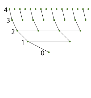
Figure 1: Depiction of the DMERA for iterations $0$ to $4$. The circles (green, filled) denote the system qubits. The thick, black lines indicate where a qubit goes from one iteration to the next and the thin, gray lines indicate which qubits are neighbors at a given iteration. The digits, always next to the first qubit, indicate the iteration.

Let us start with the number of unitaries in the past causal cone in DMERA. Recall that when looking at what happens at each iteration in the Heisenberg picture, after discarding every second qubit present in the previous iteration, we apply a unitary circuit of $D$ layers, always with the restriction that we can only apply unitaries between qubits that are neighbors on the line. When we apply the first layer, only unitaries which act on at least one qubit in the support have a nontrivial effect. Let $R(O_{t})$ be the radius of the observable before we apply the first layer of unitaries. Then there at most $2R(O_{t})-1$ nontrivial unitaries acting on the qubits in the support and two unitaries, one to the left of the support and one to the right, that act on the qubit in the left corner of the support and the first qubit to the left of the support and analogously to the right. Thus, we conclude that as we apply the first layer, we have $2R(O_{t})+1$ unitaries acting nontrivially and the support will increase to one qubit to the right and one qubit to the left. The next layer of the unitary circuit will then act on an observable of support with radius at most $R(O_{t})+1$. Applying the same reasoning as before, we see that the total number of unitaries that act nontrivially is $2R(O_{t})+3$. We conclude that the total number of unitaries that acts nontrivially after repeating this process $D$ times is bounded by:

$$\sum_{k=0}^{D-1}(2R(O_{t})+2k+1)=D(2R(O_{t})+D).$$ (1)

Let us now estimate the size of the radius at each iteration to obtain a more concrete bound on the number of unitaries.

As we observed above, if at the beginning of an iteration the radius is $R(O_{t})$, it will increase by $D$ and then be halved after we discard the qubits. Thus, it will go from $R(O_{t})$ to at most $\lceil(R(O_{t})+D)/2\rceil\leq(R(O_{t})+D)/2+1$. Applying this recursive relation, we see that if the initial radius is $R(O_{T})$ then at iteration $t$, the radius is bounded by

$$R(O_{t})\leq R(O_{T})2^{-(T-t)}+\sum\limits_{k=t}^{T}\frac{D+2}{2^{T-k}}=R(O_{T})2^{-(T-t)}+(D+2)(2-2^{-(T-t)}).$$

Note that this implies that the radius of an observable is bounded by a constant independent of $t$. Combining the bound above on the radius of the observable with Eq. (1), we obtain that the number of unitaries added to the cone at iteration $t$ is bounded by:

$$D(2R(O_{T})2^{-(T-t)}+2(D+2)(2-2^{-(T-t)})+D).$$ (2)

From this we can easily bound the total number of unitaries in the past causal cone from iteration $t$ to $T$ by summing the contribution at each step:

$$N_{U}(t,R(O_{T}))\leq\sum\limits_{k=t}^{T}D(2R(O_{k})+D)\leq\sum\limits_{k=t}^{T}D(2R(O_{T})2^{-(T-k)}+2(D+2)(2-2^{-(T-k)})+D)$$ (3)

$$\leq(T-t)D(2R(O_{T})+5D+8).$$

Let us now estimate the number of qubits in the past causal cone. At every iteration, we grow the support by at most $D$ new qubits to the left and $D$ to the right, and we start with at most $2R(O_{T})$ qubits. This leads to the bound

$$N_{Q}(t,R(O_{T}))\leq 2R(O_{T})+2D(T-t)$$ (4)

We will now estimate the error of implementing the past causal cone from iteration $t$ to $T$, which, as explained in the main text, can be bounded by:

$$2\delta(t,r)+\sum_{k=t+1}^{T}\delta(k,r)\left[\epsilon_{U}\left(N_{U}(k,r)-N_{U}(k+1,r)\right)+\epsilon_{P}\left(N_{Q}(k,r)-N_{Q}(k+1,r)\right)\right],$$ (5)

where we assume that each unitary is implemented with an error of $\epsilon_{U}$ in the $1\to 1$ norm  and we can initialize each qubit up to an error $\epsilon_{P}$, in the sense that we can prepare a state that is $\epsilon_{P}$ close in trace distance to the ideal one.

Let us start by estimating the error stemming from the noisy unitaries. Note that the term $N_{U}(k,r)-N_{U}(k+1,r)$ is nothing but the newly added unitaries at iteration $k$, which we bounded in Eq. (2). It follows that the contribution to the error from the noisy unitaries from iteration $t$ to $T$ is bounded by

$$\epsilon_{U}\sum\limits_{k=t}^{T}\left[N_{U}(k,R(O_{T}))-N_{U}(k+1,R(O_{T}))\right]\delta(k,R(O_{T}))\leq\epsilon_{U}\sum\limits_{k=t}^{T}D(2R(O_{T})+5D+8)\delta(k,R(O_{T})).$$ (6)

To illustrate the bound, we assume that $\delta(k,r)=e^{-\lambda(T-k)}$. Consequently,

$$\epsilon_{U}\sum\limits_{k=t}^{T}D(2R(O_{T})+5D+8)e^{-\lambda(T-k)}=\epsilon_{U}\frac{D(e^{\lambda}-e^{-(T-t)\lambda})(2R(O_{T})+5D+8)}{e^{\lambda}-1}.$$ (7)

One can do a similar computation for state preparation errors. As discussed above, at most $2D$ qubits are added to the causal cone for each iteration. Thus, the error caused by initialization between iterations $t$ and $T$ is bounded by:

$$\epsilon_{P}\left(2R(O_{T})+2D\sum_{k=t}^{T}e^{-\lambda(T-t)}\right)=\epsilon_{P}\left(2R(O_{T})+2D\frac{\left(e^{\lambda}-e^{-(T-t)\lambda}\right)}{e^{\lambda}-1}\right).$$ (8)

From combining equations (7) and (8), we can conclude that the error in estimating the expectation value of an observable by implementing the past causal cone from iteration $t$ to $T$ is bounded by:

$$\epsilon_{U}\frac{D(e^{\lambda}-e^{-(T-t)\lambda})(2R(O_{T})+5D+8)}{e^{\lambda}-1}+\epsilon_{P}\left(2R(O_{T})+2D\frac{\left(e^{\lambda}-e^{-(T-t)\lambda}\right)}{e^{\lambda}-1}\right)+2e^{-\lambda(T-t)}.$$

Let us now suppose we only implement the past causal cone from iterations $t_{\epsilon_{U}}=T-\lambda^{-1}\log(\epsilon_{U}^{-1})$ until $T$. The resulting error will then be at most

$$\epsilon_{U}\left(\frac{D(e^{\lambda}-\epsilon_{U})(2R(O_{T})+5D+8)}{e^{\lambda}-1}+2\right)+\epsilon_{P}\left(2R(O_{T})+2D\frac{\left(e^{\lambda}-\epsilon_{U}\right)}{e^{\lambda}-1}\right).$$

By approximating $(e^{\lambda}-1)^{-1}$ by $\lambda^{-1}$, we see that the error stemming from the noisy unitaries is at most of order $\epsilon_{U}D^{2}\lambda^{-1}$. Similarly, the error from noisy initialization of qubits is at most of order $\epsilon_{P}\lambda^{-1}D$. Moreover, by inserting $t_{\epsilon_{U}}$ into Eq. (4), we obtain that the total number of qubits necessary to perform this computation is at most

$$2R(O_{T})+2D\lambda^{-1}\log(\epsilon_{U}^{-1})$$

and the number of unitaries that needs to be implemented is bounded by

$$\lambda^{-1}\log(\epsilon_{U}^{-1})D(2R(O_{T})+5D+8),$$

which follows from inserting $t_{\epsilon_{U}}$ into Eq. (3). Thus, under these assumptions it possible to compute local expectation values of fixed radius with noisy circuits whose error and size only depends on $\lambda$ and $D$, not $T$.

Another important subclass of states are those that are sequentially generated. The most prominent example is matrix product states (MPS). Here, only one qubit interacts with the bath at each iteration. A simple generalization of this is where a group of qubits (arranged according to a $d-$dimensional graph) interacts with a bath (arranged according to a $d^{\prime}$-dimensional graph) at each iteration, see Supplementary Figure 2 for an example with $d=0$ and $d^{\prime}=2$. For this work, we also make the restriction that the interaction is given by a circuit of depth at most $D$. Setting $d=0$ and $d^{\prime}=1$, i.e. a qubit interacting with qubits on a line, recovers our version of MPS. We will also discuss the case of $d=d^{\prime}$ in more detail, which we will refer to as RI-$d$. The of case $d=d^{\prime}=1$ encapsulates examples like holographic computation discussed in Kim (2017b).

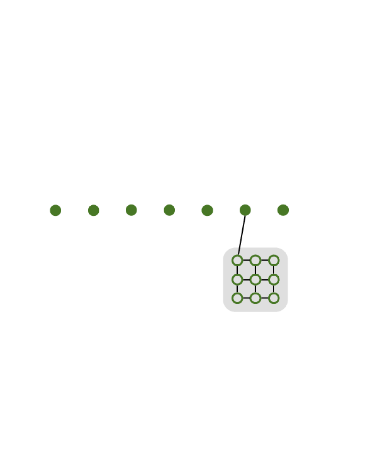
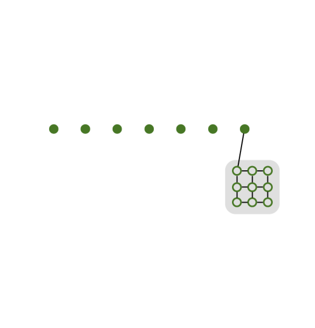
Figure 2: Three subsequent iterations of a repeated interaction system with $d=0$ and $d^{\prime}=2$. That is, the system qubits (green, filled circles) interact at each iteration with bath qubits (green, empty circles) that are arranged according to a two dimensional graph. The black, thick line indicates which system qubits is interacting with the bath, while the bath qubits interact with nearest neighbors.

We now discuss the growth of scaling of the errors in both our version of MPS and RI-$d$. Unlike we did for DMERA, we will not fix the exact graph that models the interactions in the bath and between system and bath at each iteration and choose to focus on the scaling of the size of causal cones. More precisely, we will assume that there are constants $C_{V}$ and $C_{E}$ such that for every ball of radius $r$ in the interaction graph there are at most $C_{E}r^{d}$ edges and $C_{V}r^{d}$ vertices inside the ball.

Let us now analyse the growth of causal cones. As it was the case with DMERA, if at the beginning of iteration $t$ the radius of an observable is $R(O_{t})$, it will then grow to at most $R(O_{t})+D$. However, unlike for DMERA, for the interaction schemes considered here we do not discard qubits between different iterations. Thus, the radius at iteration $t$ of an observable is bounded by $R(O_{T})+(T-t)D$. This allows us to conclude that the number of qubits in the past causal cone is bounded by:

$$N_{Q}(t,R(O_{T}))\leq C_{V}(R(O_{T})+(T-t)D)^{d}$$

for RI-$d$ and $C_{V}(R(O_{T})+(T-t)D)$ for MPS. Let us now do a similar computation for the number of unitaries in the past causal cone. Supposing that the radius of the observable is $R(O_{t})$ at the beginning of the iteration, there are at most $C_{E}(R(O_{t})+1)^{d}$ unitaries that act nontrivially on the first layer and the radius will grow by one. For the second layer, there will be at most $C_{E}(R(O_{t})+2)^{d}$ and the radius will again grow by one. We conclude that applying the $D$ layers will require a total of at most

$$C_{E}\sum\limits_{k=0}^{D-1}(R(O_{t})+k+1)^{d}$$ (9)

unitaries for iteration $t$. As $(R(O_{t})+k+1)^{d}$ is monotone increasing in $k$, we have that the number of unitaries added at each iteration is bounded by:

$$C_{E}\sum\limits_{k=0}^{D-1}(R(O_{t})+k+1)^{d}\leq C_{E}\int\limits_{1}^{D}(R(O_{t})+x+1)^{d}dx=\frac{C_{E}}{d+1}\left[\left(R(O_{t})+D+1\right)^{d+1}-\left(R(O_{t})+2\right)^{d+1}\right]$$

$$\leq \frac{C_{E}}{d+1}\left[\left(R(O_{T})+(T-t+1)D+1\right)^{d+1}-\left(R(O_{T})+(T-t)D+1\right)^{d+1}\right],$$

where for the last inequality we used our estimate for the radius of the observable at iteration $t$ and the fact that the function $x\mapsto\left(x+D+1\right)^{d+1}-\left(x+2\right)^{d+1}$ is monotone increasing for $x\geq 0$ and $D\geq 1$, as can be seen by a direct inspection of its derivative. Thus, we can bound the maximum number of unitaries in the causal cone between iteration $t$ and $T$ by:

$$N_{U}(t,r)\leq\frac{C_{E}}{d+1}\sum_{k=t}^{T}\left[\left(R(O_{T})+(T-k+1)D+1\right)^{d+1}-\left(R(O_{T})+(T-k)D+1\right)^{d+1}\right].$$ (10)

Let us now estimate this sum. To this end, define the function $f(x)=\left(R(O_{T})+xD+1\right)^{d+1}$. By the mean value theorem there exists $\xi_{k}\in[T-k,T-k+1]$ such that:

$$f(T-k+1)-f(T-k)=f^{\prime}(\xi_{k})=(d+1)D\left(R(O_{T})+\xi_{k}D+1\right)^{d}\leq(d+1)D\left(R(O_{T})+(T-k+1)D+1\right)^{d}.$$ (11)

Thus, inserting this bound into (10) it follows that

$$N_{U}(t,r)\leq C_{E}(d+1)\sum_{k=t}^{T}D\left(R(O_{T})+(T-k+1)D+1\right)^{d}\leq(d+1)C_{E}D\int\limits_{1}^{(T-t)+2}\left(R(O_{T})+xD+1\right)^{d}dx$$

$$=C_{E}\left[\left(R(O_{T})+(T-t+2)D+1\right)^{d+1}-\left(R(O_{T})+D+1\right)^{d+1}\right].$$

In particular, for MPS this gives a bound of

$$N_{U}(t,r)\leq C_{E}\left[\left(R(O_{T})+(T-t+2)D+1\right)^{2}-\left(R(O_{T})+D+1\right)^{2}\right].$$

We now assume that $\delta(t,r)=e^{-(T-t)\lambda}$ to bound the estimation error from implementing the past causal cone, as we did with DMERA. Recall that we bounded the number of new unitaries in the past causal cone at each iteration in Eq. (11). Once again, combining these estimates with our assumption on the mixing rate function and (5) yields a bound on the error stemming from the unitaries of at most

$$\epsilon_{U}C_{E}\sum\limits_{k=t}^{T}D(d+1)\left(R(O_{T})+(T-k+1)D+1\right)^{d}e^{-\lambda(T-k)}.$$

Let us now estimate this sum. First, define the function

$$g(x)=\left(R(O_{T})+xD+1\right)^{d}e^{-\lambda x}.$$

We have:

$$g^{\prime}(x)=\left(R(O_{T})+xD+1\right)^{d-1}e^{-\lambda x}\left(dD-\lambda\left(R(O_{T})+xD+1\right)\right)$$

For $x\geq 0$, we see that the function is monotone increasing for

$$x\leq x_{0}:=\frac{1}{D}\left(\frac{dD}{\lambda}-R(O_{T})-1\right)$$

and monotone decreasing for $x\geq x_{0}$. This allow us to conclude that:

$$\epsilon_{U}C_{E}\sum\limits_{k=t}^{T}D(d+1)\left(R(O_{T})+(T-k+1)D+1\right)^{d}e^{-\lambda(T-k)}\leq\epsilon_{U}C_{E}D(d+1)\left[\int\limits_{0}^{\lceil x_{0}\rceil}g(x)dx+\int\limits_{\lfloor x_{0}\rfloor}^{T-t+1}g(x)dx\right]$$ (12)

$$\leq 2\epsilon_{U}C_{E}D(d+1)\int\limits_{0}^{T-t+1}g(x)dx.$$ (13)

It now remains to estimate this integral. It is easy to compute the integral above using integration by parts $d$ times, although the resulting expressions are quite involved. We only reproduce them for $d=1$ and $d=2$ here. For $d=1$ we have:

$$\int\limits_{0}^{T-t+1}(R(O_{T})+(x+1)D)e^{-\lambda x}dx=\frac{1-e^{-\lambda(T-t+1)}}{\lambda^{2}}\left(\lambda R(O_{T})+D\lambda+D\right)-\lambda^{-2}e^{-\lambda(T-t+1)}\left(D\lambda(T-t+1)\right),$$ (14)

and for $d=2$ we obtain:

$$\frac{1-e^{-\lambda(T-t+1)}}{\lambda^{3}}\left(\lambda^{2}(D+R(O_{T}))^{2}+2\lambda D(D+R(O_{T}))+2D^{2}\right)$$ (15)

$$-\lambda^{-3}e^{-\lambda(T-t+1)}\left(2\lambda^{2}D(R(O_{T})+D)(T-t+1)+D^{2}\lambda^{2}(T-t+1)^{2}\right).$$

It is then possible to obtain explicit bounds by combining the equations above with Eq. (12). But it is easy to see by direct inspection that, assuming $R(O_{T})\leq D$, the error will converge exponentially fast in $(T-t)$ to $\mathcal{O}\left(\epsilon_{U}C_{E}\left(D\lambda^{-1}\right)^{d+1}\right)$, which is again independent of $T$. It is also possible to obtain more explicit bounds on the asymptotic behaviour of the error, i.e. with $T\to\infty$. To this end, note that $g(x)\geq 0$, thus:

$$\int_{0}^{T-t+1}g(x)dx\leq\int_{0}^{+\infty}\left(R(O_{T})+xD+1\right)^{d}e^{-\lambda x}dx=D^{-1}\int\limits_{R(O_{T})+1}^{\infty}y^{d}e^{-\frac{\lambda}{D}\left(y-R(O_{T}-1)\right)}dy$$

$$\leq D^{-1}\int\limits_{0}^{\infty}y^{d}e^{-\frac{\lambda}{D}\left(y-R(O_{t}-1)\right)}dy=\frac{e^{\frac{\lambda}{D}\left(R(O_{T})+1\right)}}{D}\int\limits_{0}^{+\infty}y^{d}e^{-\frac{\lambda}{D}\left(y\right)}dy=\frac{D^{d}e^{\frac{\lambda}{D}\left(R(O_{T})+1\right)}}{\lambda^{d+1}}\int\limits_{0}^{+\infty}z^{d}e^{-z}dz=\frac{d!D^{d}e^{\frac{\lambda}{D}\left(R(O_{T})+1\right)}}{\lambda^{d+1}}.$$

This allows us to conclude that the noise stemming from the noisy unitaries is bounded by:

$$2C_{E}\epsilon_{U}\frac{(d+1)!D^{d+1}e^{\frac{\lambda}{D}\left(R(O_{T})+1\right)}}{\lambda^{d+1}}.$$

Similar estimates hold for the total initialization errors ($\epsilon_{P}$). We see that the number of qubits added at iteration $t$ is bounded by:

$$(R(O_{T})+(T-t+1)D)^{d}-(R(O_{T})+(T-t)D)^{d}\leq dD(R(O_{T})+(T-t+1)D)^{d-1},$$

again using the mean value theorem. Thus, we may estimate the initialization error by:

$$\epsilon_{P}C_{V}dD\sum\limits_{k=t}^{T}(R(O_{T})+(T-k+1)D)^{d-1}e^{-\lambda t}.$$ (16)

The attentive reader must have already realized that the expression in (12) coincides with that of (16) up to a constant if replace $d+1$ by $d$. Thus, we may use the same estimation techniques and conclude that the error is bounded by $\mathcal{O}\left(\epsilon_{P}C_{V}\left(D\lambda^{-1}\right)^{d}\right)$. Moreover, we may resort to the expressions in (14) and (15) if more refined inequalities in terms of $t$ and $R(O_{T})$ are desired. Thus, the total error of implementing the causal cone from $T-t$ to $t$ is bounded by:

$$2C_{V}\epsilon_{P}\frac{d!D^{d}e^{\frac{\lambda}{D}\left(R(O_{T})+1\right)}}{\lambda^{d}}+2C_{E}\epsilon_{U}\frac{(d+1)!D^{d+1}e^{\frac{\lambda}{D}\left(R(O_{T})+1\right)}}{\lambda^{d+1}}+2e^{-\lambda(T-t)},$$

up to corrections that are exponentially small in $T-t$.

I.2 Mixing rates of quantum channels

In this subsection, we clarify the connections between the mixing rate function and the mixing properties of quantum channels Burgarth et al. (2013).

Definition 1 (Mixing quantum channel).

A quantum channel $\Lambda:\mathcal{M}_{d}\to\mathcal{M}_{d}$ is called mixing if there is a unique state $\sigma$ such that $\Lambda(\sigma)=\sigma$ and for all states $\rho$ we have that

$$\lim\limits_{n\to\infty}\Lambda^{n}(\rho)=\sigma,$$

where $\Lambda^{n}$ denotes the quantum channel composed with itself $n$ times.

Given a mixing quantum channel $\Lambda$, the main quantity of interest is $t_{1}(\epsilon)$, defined as

$$t_{1}(\epsilon)=\inf\{n|\sup_{\rho}\|\Lambda^{n}\left(\rho\right)-\sigma\|_{1}\leq\epsilon\}.$$

For $\epsilon>0$ this quantity measures how long it takes for the quantum channel to converge, i.e., its mixing time Burgarth et al. (2013); Temme et al. (2010). Here $\|\cdot\|_{1}$ corresponds to the trace norm. It is well-known that correlations in tensor network or finitely correlated states are governed by mixing properties of the transfer operator Fannes et al. (1992); Perez-Garcia et al. (2006). We will now show this connection for completeness of the exposition.

Note that

$$\sup\limits_{\rho}\|\Lambda^{n}(\rho)-\sigma\|_{1}$$

corresponds to the $1\to 1$ norm of the linear operator $\Lambda-\Lambda_{\infty}$, where $\Lambda_{\infty}(\rho)=\text{tr}(\rho)\sigma$. It follows from duality that:

$$\|\Lambda^{n}-\Lambda_{\infty}\|_{1\to 1}=\|(\Lambda^{n})^{*}-\Lambda_{\infty}^{*}\|_{\infty\to\infty}$$

and $\Lambda^{*}_{\infty}(O)=\text{tr}(\sigma O)\mathbb{1}$. Now suppose, for simplicity, that we wish to compute the expectation value of an observable $O$ supported on one qubit in $S_{T}$ and our interaction scheme is that of MPS. In this case, the qubits only interact with the bath at each iteration and not each other. Moreover, let us assume that the system is translationally invariant in the sense that we assume that $\mathcal{U}_{t}$ is the same for all $t$. Now note that

$$O_{T}=\Phi_{T}^{*}(O)=\text{tr}_{S_{T}A_{T}}\left(\mathcal{U}_{T}^{*}\left(O\otimes\mathbb{1}_{S_{1}\ldots S_{T-1}S_{B}}\right)\right).$$

will be an observable supported on the bath alone. Furthermore,

$$\Phi_{t}^{*}(O_{t+1})=\text{tr}_{S_{t}A_{t}}\left(\mathcal{U}_{t}^{*}\left(O_{t+1}\otimes\mathbb{1}_{S_{1}\ldots S_{t}}\right)\right).$$

Since we have assumed the action of all $\mathcal{U}_{t}$ to be the same, we may define the quantum channel $\Lambda_{B}^{*}$ from the bath to itself as

$$\Lambda_{B}^{*}(X)=\text{tr}_{S_{t}A_{t}}\left(\mathcal{U}_{t}^{*}\left(X\otimes\mathbb{1}_{S_{1}\ldots S_{t}}\right)\right).$$

We then have that $O_{t}=\left(\Lambda_{B}^{*}\right)^{T-t}(O_{1})$. If $\Lambda_{B}$ is mixing, which is the generic case Burgarth et al. (2013), we may directly bound the mixing rate with a mixing time bound on $\Lambda_{B}$. Let

$$\mathcal{B}_{r}=\{O:R(O)\leq r,\|O\|_{\infty}\leq 1\}.$$

Observe that

$$\delta(t,r)=\sup\limits_{O\in\mathcal{B}_{r}}\inf_{c\in\mathds{R}}\|\Phi^{*}_{[t,T]}\left(O\right)-c\mathbb{1}\|_{\infty}=\sup\limits_{O\in\mathcal{B}_{r}}\inf_{c\in\mathds{R}}\|\left(\Lambda_{B}^{*}\right)^{T-t}(O)-c\mathbb{1}\|_{\infty}.$$

For $\Lambda_{B}$ mixing, a natural choice for the constant $c$ is given by $\text{tr}\left(O_{1}\sigma\right)$, as in this case we have:

$$\delta(t,r)\leq\sup\limits_{\mathcal{B}_{r}}\|\left(\Lambda_{B}^{*}\right)^{T-t-1}(O_{1})-\text{tr}\left(O_{1}\sigma\right)\mathbb{1}\|_{\infty}\leq\|\Lambda_{B}^{T-t-1}-\Lambda_{B,\infty}\|_{1\to 1}.$$

We conclude that in this case, $\delta(l,r)$ can be bounded using mixing time techniques Burgarth et al. (2013); Temme et al. (2010); Reeb et al. (2011); Bardet (2017); Müller-Hermes and Franca (2018). But note that these might provide a too pessimistic bound on $\delta(l,r)$, as they do not take into account the radius of the support $r$.

Although we made the restrictive assumption that all $\mathcal{U}_{t}$ are the same, it is straightforward to adapt the arguments above to the case where they are different. This, however, implies that the sequence of quantum channels of interest is not homogeneous in time. It is, in general, not known how to estimate the convergence or even certify convergence for a non-homogeneous sequence. One important exception is when the quantum channels change adiabatically in time Hanson et al. (2017). Moreover, the results of Refs. González-Guillén et al. (2018); Lancien and Pérez-García (2019) seem to indicate that we should expect an exponential decay of the mixing rate function for generic local circuits of logarithmic depth in the number of qubits, but we leave this investigation for future work. Finally, we note that it is straightforward to adapt our results to the case in which the the unitary channel $\mathcal{U}_{t}$ depends on a classical random variable. That is, we apply some quantum channel $\mathcal{T}_{t}$ which is a convex combination of unitaries respecting the locality. This leads to a richer variety of evolutions that can be implemented (see e.g. Iten et al. (2016)) and can be used to ensure rapid mixing.

I.3 Correlation length of the produced states

Here we discuss how the mixing rate function $\delta(t,r)$ and the geometry of the interaction scheme can be used to bound the correlations present in the state produced. We measure the correlations in the state in terms of the covariance, which we introduce below.

Definition 2 (Covariance).

Let $E,F$ be observables with disjoint support in $G_{T}$. Their covariance with respect to a state $\rho$, $\operatorname{cov}_{\rho}(E,F)$, is defined as:

$$\operatorname{cov}_{\rho}(E,F)=\text{tr}\left(\rho E\otimes F\right)-\text{tr}\left(\rho E\right)\text{tr}\left(\rho F\right).$$

We then have:

Proposition (Correlations of the state).

Let $E$ and $F$ be observables whose support is disjoint and contained in a ball of radius $r$ and $\rho=\Phi_{[0,T]}(\rho_{0}\otimes\rho_{B})$. Moreover, let $t_{0}$ be the largest $t$ s.t. $E_{t}$ and $F_{t}$ have supports that intersect. Then

$$\left|\operatorname{cov}_{\rho}(E,F)\right|\leq 6\delta(t_{0},r)\|E\|_{\infty}\|F\|_{\infty}.$$

Proof.

Note that for $t>t_{0}$ the supports of $E_{t}$ and $F_{t}$ are disjoint by definition, that is, $\Phi_{[t,T]}^{*}(E\otimes F)$ are still product observables. By the definition of the mixing rate, there are constants $c_{E}$ and $c_{F}$ such that:

$$\Phi_{[t,T]}^{*}(E\otimes F)=\left(c_{E}\mathbb{1}+\delta(t,r)E^{\prime}_{t}\right)\otimes\left(c_{F}\mathbb{1}+\delta(t,r)F^{\prime}_{t}\right).$$

Here $E^{\prime}$ is an observable satisfying $\|E^{\prime}_{t}\|_{\infty}\leq\|E\|_{\infty}$ and whose support is contained in the support of $E_{t}$. Analogous properties apply to $F^{\prime}_{t}$. Moreover, note that $c_{E}\leq\|E\|_{\infty}$. Defining

$$\tilde{C}=\Phi_{[t,T]}^{*}(\left(c_{E}\mathbb{1}\otimes\delta(t,r)F^{\prime}_{t}\right)+\left(\delta(t,r)E^{\prime}_{t}\otimes c_{F}\mathbb{1}\right)+\delta(t,r)E^{\prime}_{t}\otimes\delta(t,r)F^{\prime}_{t})$$

we have that

$$\text{tr}\left(\rho E\otimes F\right)= \text{tr}\left(\rho_{0}\otimes\rho_{B}\Phi_{[0,T]}^{*}(E\otimes F)\right)=c_{E}c_{F}+\text{tr}\left(\tilde{C}\rho_{0}\otimes\rho_{B}\right).$$

An application of the triangle inequality yields $\|\tilde{C}\|_{\infty}\leq 3\delta(t,r)\|E\|_{\infty}\|F\|_{\infty}$, from which we conclude

$$\left|\text{tr}\left(\rho E\otimes F\right)-c_{E}c_{F}\right|\leq 3\delta(t,r)\|E\|_{\infty}\|F\|_{\infty}.$$ (17)

A similar computation yields that

$$\Phi_{[t,T]}^{*}(E\otimes\mathbb{1})=\left(c_{E}+\delta(t,r)E^{\prime}_{t}\right)\otimes\mathbb{1},\quad\Phi_{[t,T]}^{*}(\mathbb{1}\otimes F)=\mathbb{1}\otimes\left(c_{F}+\delta(t,r)F^{\prime}_{t}\right).$$

We, therefore, have that

$$\text{tr}\left(\rho E\right)=c_{E}+\text{tr}\left(\rho_{0}\otimes\rho_{B}\tilde{C}_{E}\right),\quad\text{tr}\left(\rho F\right)=c_{F}+\text{tr}\left(\rho_{0}\otimes\rho_{B}\tilde{C}_{F}\right),$$ (18)

where $\tilde{C}_{E}=\delta(t,r)\Phi_{[t,T]}^{*}\left(E^{\prime}_{t}\right)$ and $\tilde{C}_{F}$ is defined analogously. From (18) we conclude that:

$$|\text{tr}\left(\rho E\right)\text{tr}\left(\rho F\right)-c_{E}c_{F}|\leq 3\delta(t,r)\|E\|_{\infty}\|F\|_{\infty}.$$

Combining the last inequality with (17) we finally have that:

$$\left|\text{tr}\left(\rho E\right)\text{tr}\left(\rho F\right)-\text{tr}\left(\rho E\otimes F\right)\right|\leq|\text{tr}\left(\rho E\right)\text{tr}\left(\rho F\right)-c_{E}c_{F}|+|\text{tr}\left(\rho E\otimes F\right)-c_{E}c_{F}|\leq 6\delta(t,r)\|E\|_{\infty}\|F\|_{\infty}.$$

∎

I.4 Connection to the results of Kim et al

First, we briefly review our assumptions on the noise in the implementation, which are closely related to that of Kim et al. Kim (2017a); Kim and Swingle (2017). Like them, we assume that noisy versions $\mathcal{N}_{U}$ of the required two qubit gates $U$ are implemented, which satisfy:

$$\|\mathcal{U}-\mathcal{N}_{U}\|_{\diamond}\leq\epsilon_{U}.$$ (19)

and the noise acts on the same qubits as $U$. Here $\mathcal{U}$ is just the quantum channel that corresponds to conjugation with $U$ and $\|\cdot\|_{\diamond}$ is the diamond norm. Recall that the diamond norm is defined as

$$\|\Lambda\|_{\diamond}=\sup\limits_{X\in\mathcal{M}_{n}\otimes\mathcal{M}_{n}}\frac{\|\Lambda\otimes\textrm{id}\left(X\right)\|_{1}}{\|X\|_{1}}$$

for a linear operator $\Lambda:\mathcal{M}_{n}\to\mathcal{M}_{n}$ and $\|\cdot\|_{1}$ the trace norm. The diamond norm is a natural way of quantifying the noise in our setting as it also allows us to estimate its effect on systems other than the one the unitary is acting on. However, it should be noted that as all unitaries considered in this work only act nontrivially on two qubits, the diamond norm can differ by at most a factor of $4$ from $\|\cdot\|_{1\to 1}$. That is,

$$\epsilon_{U}\leq 4\|\mathcal{U}-\mathcal{N}_{U}\|_{1\to 1}.$$

We also assume that the initial state preparation is noisy. This can be modelled similarly by assuming further that all qubits are initialized in a state that is $\epsilon_{P}$ in trace distance to the ideal one. Let us now connect the mixing rate function of circuits to stability bounds of noisy implementations, which will allow us to recover (Kim, 2017a, Theorem 2) in our language.

Corollary (Stability of noisy implementation).

Let

$$\rho=\text{tr}_{B}\left[\Phi_{[0,T]}\left(\rho_{0}\otimes\rho_{B}\right)\right]$$

and $\tilde{\rho}$ be the quantum state obtained by replacing every two qubit unitary in $\Phi_{t}$ by a noisy counterpart satisfying (19) and every qubit initialized up to a preparation error of $\epsilon_{P}$. Moreover, let $O$ be an observable supported on a ball of radius $r$ and $\|O\|_{\infty}\leq 1$. Then for all $0\leq t\leq T$:

$$|\text{tr}\left(O\left(\rho-\tilde{\rho}\right)\right)|\leq\delta(t,r)+\sum_{k=t+1}^{T}\delta(k,r)\left[\epsilon_{U}\left(N_{U}(k,r)-N_{U}(k+1,r)\right)+\epsilon_{P}\left(N_{Q}(k,r)-N_{Q}(k+1,r)\right)\right].$$ (20)

Proof.

Let $\tilde{\Phi}_{t}$ be the noisy counterpart of $\Phi_{t}$. As in (Kim, 2017a, Theorem 2), we now consider the decomposition

$$\Phi_{[0,T]}^{*}-\tilde{\Phi}_{[0,T]}^{*}=\left(\Phi_{[0,t-1]}^{*}-\tilde{\Phi}_{[0,t-1]}^{*}\right)\circ\Phi_{[0,t]}^{*}+\sum\limits_{k=t}^{T}\tilde{\Phi}_{[0,k-1]}^{*}\circ\left(\Phi_{k}^{*}-\tilde{\Phi}_{k}^{*}\right)\circ\Phi_{[k+1,T]}^{*},$$

with the convention that $\Phi_{[-1,0]}^{*},\Phi_{[T+1,T]}^{*}$ are the identity. Let us first estimate the error from the sum by estimating each summand. First, note that, as before, we have:

$$\Phi_{[k+1,T]}^{*}(O)=\delta(k+1,r)A_{k+1}+c_{k+1}\mathbb{1},$$

where once again we have $\|A_{k+1}\|_{\infty}\leq\|O\|_{\infty}$ with the same support as $O_{k+1}$ and $c_{k+1}$ is some constant. Moreover, $\left(\Phi_{k}^{*}-\tilde{\Phi}_{k}^{*}\right)$ will map the identity to $0$. Thus,

$$\|\tilde{\Phi}_{[0,k-1]}^{*}\circ\left(\Phi_{k}^{*}-\tilde{\Phi}_{k}^{*}\right)\circ\Phi_{[k+1,T]}^{*}\left(O\right)\|_{\infty}=\delta(k+1,r)\|\tilde{\Phi}_{[0,k-1]}^{*}\circ\left(\Phi_{k}^{*}-\tilde{\Phi}_{k}^{*}\right)\left(A_{k+1}\right)\|_{\infty}$$ (21)

As we assumed that the noise is local, that is, it acts on the same qubits as the two-qubit gate  the action of $\tilde{\Phi}_{k}$ and $\Phi_{k}$ will be identical outside the support of $A_{k+1}$. This is because both will just map the identity to the identity outside the support. This implies that only the unitary gates in the past causal cone of the observable contribute to the error and each one by $\epsilon_{U}$. A similar argument holds for the qubit initialization errors, as only erroneous initialization on the past causal cone contribute to the error. As there are at most $N_{U}(t-1,r)-N_{U}(t,r)$ new unitaries at iteration $t-1$ and at most $N_{Q}(t-1,r)-N_{Q}(t,r)$ new qubits, we conclude that:

$$\|\tilde{\Phi}_{[0,k-1]}^{*}\circ\left(\Phi_{k}^{*}-\tilde{\Phi}_{k}^{*}\right)\left(A_{k+1}\right)\|_{\infty}\leq\epsilon_{U}\left(N_{U}(k+1,r)-N_{U}(k,r)\right)+\epsilon_{P}\left(N_{Q}(k+1,r)-N_{Q}(k,r)\right)$$ (22)

Thus, combining (21) and (22) yields:

$$\|\sum\limits_{k=t}^{T}\tilde{\Phi}_{[0,k-1]}^{*}\circ\left(\Phi_{k}^{*}-\tilde{\Phi}_{k}^{*}\right)\circ\Phi_{[k+1,T]}^{*}\left(O\right)\|_{\infty}\leq\sum\limits_{k=t}^{T}\delta(k+1,r)\|\tilde{\Phi}_{[0,k-1]}^{*}\circ\left(\Phi_{k}^{*}-\tilde{\Phi}_{k}^{*}\right)\left(A_{k+1}\right)\|_{\infty}$$

$$\leq\sum_{k=t}^{T}\delta(k+1,r)\left[\epsilon_{U}\left(N_{U}(k,r)-N_{U}(k+1,r)\right)+\epsilon_{P}\left(N_{Q}(k,r)-N_{Q}(k+1,r)\right)\right]$$

Now, by the definition of the mixing rate function there exists an observable $A$ such that

$$\Phi_{[k,T]}(O)=c\mathbb{1}+\delta(k,r)A$$

with $\|A\|_{\infty}\leq 1$. Thus, we see that

$$\left(\Phi_{[0,k-1]}^{*}-\tilde{\Phi}_{[0,k-1]}^{*}\right)\circ\Phi_{[k,T]}(O)=\delta(k,r)\left(\Phi_{[0,k-1]}^{*}-\tilde{\Phi}_{[0,k-1]}^{*}\right)\circ\Phi_{[k,T]}^{*}(A),$$

as the identity is in the kernel of $\Phi_{[0,k-1]}^{*}-\tilde{\Phi}_{[0,k-1]}^{*}$. We conclude that

$$\|\Phi_{[0,T]}^{*}-\tilde{\Phi}_{[0,T]}^{*}(O)\|_{\infty}\leq\delta(t,r)+\sum_{k=t}^{T}\delta(k,r)\left[\epsilon_{U}\left(N_{U}(k,r)-N_{U}(k+1,r)\right)+\epsilon_{P}\left(N_{Q}(k,r)-N_{Q}(k+1,r)\right)\right],$$

from which the claim follows.

∎

The stability results of Refs. Kim (2017a); Kim and Swingle (2017) are captured by this corollary. For instance, the main result of Ref. Kim (2017a) follows from assuming that there exist constants $r_{0},c,k,\alpha,\Delta\geq 0$ independent of system size such that for all $r\leq r_{0}$:

$$\delta(t,r)=cr^{\alpha}e^{-\gamma(T-t)}+\Delta.$$

Optimizing

$$t_{0}=T-\frac{1}{\gamma}\log\left(\frac{\epsilon}{Dr^{\alpha}c}\right)^{2}$$

suffices to guarantee an estimate up to $\mathcal{O}\left(D^{2}\epsilon\log(\epsilon^{-1})^{2}+\Delta\right)$, as in Kim (2017a). By comparing Corollary Corollary with our main theorem (see article), we see that this stability comes from the fact that the assumptions on $\delta(t,r)$ imply that there is an ”effective” circuit of constant size underlying the computation. Moreover, each iteration of the evolution can only change the expectation value by an amount that decreases with time.

This is well illustrated when we compare the bound in Eq. (20) and the one we obtained with our main result, reproduced in the supplementary material in Eq. (5). Note that the two bounds only differ by a factor of $\delta(t,r)$. This difference has a clear interpretation in light of the discussion above: in our result we allowed for an arbitrary initial state $\tilde{\rho}$ when implementing the past causal cone from iteration $t$ to $T$ , while above the state at iteration $t$ is given by $\Phi_{[0,t-1]}(\rho_{0}\otimes\rho_{B})$ in the noiseless version. With the previous discussion in mind, we see that any change to the state produced from iteration $0$ to $t$ can only change the expectation value by $\delta(t,r)$, which explains the extra $\delta(t,r)$ factor. It is also important to note that the connection between rapid mixing under local evolutions and stability of the expectation values of local observables was established in Lucia et al. (2015); Cubitt et al. (2015), where the authors show similar results for time evolutions in continuous time.

Finally, it should be noted that our approach also requires a bound on $\delta(t,r)$ to ensure that the energy inferred from the smaller patches corresponds to a physical quantum state. This is not the case if the whole circuit or causal cone preparing the many-body state is implemented.

I.5 Certifying mixing

A close look at the proof of the main theorem shows that $\delta(t,r)$ provides a worst-case estimate for how fast the expectation values stabilize. If we are only interested in estimating the expectation value of a given observable $O$, we see that

$$\inf\limits_{c\in\mathds{R}}\|O_{t}-c\mathbb{1}\|_{\infty}$$

gives an upper bound on the error we obtain when we estimate $\text{tr}(\rho O)$ by only implementing the circuit from iteration $t$ to $T$. Thus, it is not necessary to bound the mixing rate for arbitrary observables, which is expected to be hard in general. E.g. the results of Bookatz et al. (2013) show that it is QMA-hard to determine the spectral gap Temme et al. (2010) of certain quantum channels, which is a central quantity in determining the mixing time of quantum channels. We will therefore focus on bounding the mixing for a given observable $O$. We will show that in case $\operatorname{supp}O_{t}$ is small it is possible to bound $\|O_{t}-c\mathbb{1}\|_{\infty}$ on a quantum computer.

As can be seen in the proof of the main theorem, if $\delta(t,r)$ is small, then the output of the circuit is essentially independent of the initial state. Thus, it should be expected that the dependence of the expectation value of an observable $O$ on the initial state gives an estimate on the mixing time. Indeed, if we draw a state $\sigma_{t}$ from a state two design (Ambainis and Emerson, 2007) on the support of $O_{t}$ and define the random variable $X_{t}=\text{tr}\left(\sigma_{t}O_{t}\right)$, then:

$$\left(2^{n_{t}}\left(\mathbb{E}(X_{t}^{2})\left(2^{n_{t}}+1\right)-2\mathbb{E}\left(X_{t}\right)^{2}\right)\right)^{\frac{1}{2}}\geq\|O_{t}-\text{tr}\left(\Phi^{*}_{[t,T]}\left(O\right)\right)\frac{\mathbb{1}}{2^{n_{t}}}\|_{\infty}.$$ (23)

Here $n_{t}$ is the number of qubits on the support of $O_{t}$. As it is possible to generate a two state design using $\mathcal{O}(n_{t}\log^{2}(n_{t}))$ gates Cleve et al. (2016), equation (23) gives a protocol to measure how far each local observable is from stabilizing as long as $n_{t}$ is small by estimating the first and second moments of $X_{t}$. This protocol applies to interaction schemes for which the support of observables has a bounded radius, like DMERA, otherwise the scaling in $n_{t}$ is prohibitively large.

We now discuss to derive (23) and its consequences in more detail. We start by recalling the definition of a quantum state design Ambainis and Emerson (2007):

Definition 3 (State design).

A distribution $\mu$ over the set of $d$ dimensional quantum states is called a $k-$state design for some $k>0$ if

$$\int(|\psi\rangle\langle\psi|)^{\otimes k}d\mu=\int(|\psi\rangle\langle\psi|)^{\otimes k}d\mu_{U},$$

where $\mu_{U}$ is the (normalized) uniform measure on the set of pure quantum states.

That is, these states have the same first $k$ moments as the uniform distribution on the set of pure states. Let us now compute some relevant moments of the random quantum states: Let $\ket{\psi}$ be drawn from the uniform distribution of $d-$ dimensional pure quantum states and $O$ be an observable. Moreover, define the random variable $X=\text{tr}\left(|\psi\rangle\langle\psi|O\right)$. Then:

$$\mathbb{E}(X)=\frac{\text{tr}\left(O\right)}{d},\quad\mathbb{E}(X^{2})=\frac{1}{d(d+1)}\left(\text{tr}(O^{2})+\text{tr}(O)^{2}\right).$$ (24)

This can be derived by e.g. noting that $|\psi\rangle\langle\psi|$ has the same distribution as $U|0\rangle\langle 0|U^{\dagger}$, where $U$ is a Haar random unitary. A simple application of the Weingarten calculus for the moments of the Haar measure on the unitary group Collins and Śniady (2006); Fukuda et al. (2019) yields the result. We are now ready to prove equation (23), which we restate as a lemma for the reader’s convenience:

Lemma (Checking mixing).

Let $O$ be an observable and $n_{t}$ be the number of qubits in the support of $O_{t}$. Moreover, let $\sigma_{t}$ be drawn from a state $2-$design on the support of $O_{t}$ and denote by $X_{t}$ the random variable $X_{t}=\text{tr}\left(\Phi_{[t,T]}\left(\sigma_{t}\right)O\right)$. Then

$$\left(2^{n_{t}}\left(\mathbb{E}(X^{2})\left(2^{n_{t}}+1\right)-2\mathbb{E}\left(X\right)^{2}\right)\right)^{\frac{1}{2}}\geq\|\Phi^{*}_{[t,T]}\left(O\right)-\text{tr}\left(\Phi^{*}_{[t,T]}\left(O\right)\right)\frac{\mathbb{1}}{2^{n_{t}}}\|_{\infty}.$$

Proof.

Note that

$$\left\|\Phi^{*}_{[t,T]}\left(O\right)-\text{tr}\left(\Phi^{*}_{[t,T]}\left(O\right)\right)\frac{\mathbb{1}}{2^{n_{t}}}\right\|_{F}^{2}=\text{tr}\left(\Phi^{*}_{[t,T]}\left(O\right)^{2}\right)-2^{-n_{t}}\text{tr}\left(\Phi^{*}_{[t,T]}\left(O\right)\right)^{2}.$$

Here $\|\cdot\|_{F}$ is the Frobenius norm. It follows from (24) that

$$2^{n_{t}}\left(\mathbb{E}(X^{2})\left(2^{n_{t}}+1\right)-2\mathbb{E}\left(X\right)^{2}\right)=\left\|\Phi^{*}_{[t,T]}\left(O\right)-\text{tr}\left(\Phi^{*}_{[t,T]}\left(O\right)\right)\frac{\mathbb{1}}{2^{n_{t}}}\right\|_{F}^{2}$$

if we draw $\sigma$ from the uniform distribution on states. But it is clear that the expression only depends on the second and first moments of the random variable. Thus, a state $2-$design satisfies the same properties. The claim then follows from the fact that $\|\cdot\|_{F}\geq\|\cdot\|_{\infty}$. ∎

We note that in case the quantum channel has a spectral gap, then

$$\left\|\Phi^{*}_{[t,T]}\left(O\right)-\text{tr}\left(\Phi^{*}_{[t,T]}\left(O\right)\right)\frac{\mathbb{1}}{2^{n_{t}}}\right\|_{F}^{2}$$

decays exponentially with $(T-t)$ Temme et al. (2010). As a quantum state two design of $n$ qubits can be generated with a circuit consisting of $\mathcal{O}(n\log^{2}(n))$ two-qubit gates Cleve et al. (2016). Moreover, for some $n$ there are simplified constructions of state $2$-designs that only require a circuit of linear depth and Hadamard and controlled phase gates Seyfarth and Ranade (2011). These are based on the fact any set of maximal mutually orthogonal bases also gives a two-design Klappenecker and Rotteler (2005).

Moreover, it is important to take into account the effect of noise in the evolution. As the proof above did not take into account any special property of the quantum channel itself, we can replace $\Phi^{*}_{[t,T]}$ by the noisy evolution $\tilde{\Phi}^{*}_{[t,T]}$ and the statement still holds. Thus, assuming that we implement the noisy version instead and can prepare the states in the $2$-design perfectly, the protocol above still measures how mixed the outputs of the noisy quantum computer.

Thus, it only remains to estimate the effects of noise in the preparation procedure of the $2$-design required to estimate the moments of $X_{t}$. Unfortunately, the $2^{n_{t}}$ pre-factor in the inequality above implies that the precision in the preparation of the $2-$design and number of samples required to check mixing is infeasible whenever the support of $O_{t}$ is large, as both scale exponentially with $n_{t}$.