Abstract

We provide a new analysis of local SGD, removing unnecessary assumptions and elaborating on the difference between two data regimes: identical and heterogeneous. In both cases, we improve the existing theory and provide values of the optimal stepsize and optimal number of local iterations. Our bounds are based on a new notion of variance that is specific to local SGD methods with different data. The tightness of our results is guaranteed by recovering known statements when we plug $H=1$, where $H$ is the number of local steps. The empirical evidence further validates the severe impact of data heterogeneity on the performance of local SGD.

1 Introduction

Modern hardware increasingly relies on the power of uniting many parallel units into one system. This approach requires optimization methods that target specific issues arising in distributed environments such as decentralized data storage. Not having data in one place implies that computing nodes have to communicate back and forth to keep moving toward the solution of the overall problem. A number of efficient first-, second-order and dual methods that are capable of reducing the communication overhead existed in the literature for a long time, some of which are in certain sense optimal.

Yet, when Federated Learning (FL) showed up, it turned out that the problem of balancing the communication and computation had not been solved. On the one hand, Minibatch Stochastic Gradient Descent (SGD), which averages the result of stochastic gradient steps computed in parallel on several machines, again demonstrated its computation efficiency. Seeking communication efficiency, Konečný et al. [2016], McMahan et al. [2017] proposed to use a natural variant of Minibatch SGD—Local SGD (Algorithm 1), which does a few SGD iterations locally on each involved node and only then computes the average. This approach saves a lot of time on communication, but, unfortunately, in terms of theory things were not as great as in terms of practice and there are still gaps in our understanding of Local SGD.

The idea of local SGD in fact is not recent, it traces back to the work of Mangasarian [1995] and has since been popular among practitioners from different communities. An asymptotic analysis can be found in Mangasarian [1995] and quite a few recent papers proved new convergence results, making the bounds tighter with every work. The theory has been developing in two important regimes: identical and heterogeneous data.

The identical data regime is more of interest if the data are actually stored in one place. In that case, we can access it on each computing device at no extra cost and get a fast, scalable method. Although not very general, this framework is already of interest to a wide audience due to its efficiency in training large-scale machine learning models [Lin et al., 2020]. The first contribution of our work is to provide the fastest known rate of convergence for this regime under weaker assumptions than in prior work.

Federated learning, however, is done on a very large number of mobile devices, and is operating in a highly non-i.i.d. regime. To address this, we present the first analysis of Local SGD that applies to arbitrarily heterogeneous data, while all previous works assumed a certain type of similarity between the data or local gradients.

Algorithm 1 Local SGD

0:  Stepsize $\gamma>0$, initial vector $x_{0}=x_{0}^{m}$ for all $m\in[M]$, synchronization timesteps $t_{1},t_{2},\ldots$.

1:  for $t=0,1,\dotsc$ do

2:     for $m=1,\dotsc,M$ in parallel do

3:        Sample $z_{m}\overset{\text{i.i.d.}}{\sim}\mathcal{D}_{m}$.

4:        if data is identical then

5:           Compute $g_{t}^{m}=g(f,x_{t}^{m},z_{m})$ such that $\mathbb{E}\left[g_{t}^{m}\mid x_{t}^{m}\right]=\nabla f(x_{t}^{m})$.

6:        else

7:           Compute $g_{t}^{m}=g(f_{m},x_{t}^{m},z_{m})$ such that $\mathbb{E}\left[g_{t}^{m}\mid x_{t}^{m}\right]=\nabla f_{m}(x_{t}^{m})$.

8:        end if

9:        $x_{t+1}^{m}=\begin{cases}\frac{1}{m}\sum_{j=1}^{M}(x_{t}^{j}-\gamma g_{t}^{j}),&\text{ if }t=t_{p}\text{ for some }p\in\mathbb{N}\\ x_{t}^{m}-\gamma g_{t}^{m},&\text{ otherwise. }\end{cases}$

10:     end for

11:  end for

To explain the challenge of heterogeneity better, let us introduce the problem we are trying to solve. Given that there are $M$ devices and corresponding local losses $f_{m}:\mathbb{R}^{d}\to\mathbb{R}$, we want to find

$$\min_{x\in\mathbb{R}^{d}}\left\{f(x)=\frac{1}{M}\sum_{m=1}^{M}f_{m}(x)\right\}.$$ (1)

In the case of identical data, we are able to obtain on each node an unbiased estimate of the gradient $\nabla f$. In the case of heterogeneous data, $m$-th node can only obtain an unbiased estimate of the gradient $\nabla f_{m}$. Data similarity can then be formulated in terms of the differences between functions $f_{1},\dotsc,f_{M}$. If the underlying data giving rise to the loss functions are i.i.d., the function share optima and one could even minimize them separately, averaging the results at the end. We will demonstrate this rigorously later in the paper.

If the data are dissimilar, however, we need to be much more careful since running SGD locally will yield solutions of local problems. Clearly, their average might not minimize the true objective (1), and this poses significant issues for the convergence of Local SGD.

To properly discuss the efficiency of local SGD, we also need a practical way of quantifying it. Normally, a method’s efficiency is measured by the total number of times each function $f_{m}$ is touched and the cost of the touches. On the other hand, in distributed learning we also care about how much information each computing node needs to communicate. In fact, when communication is as expensive as is the case in FL, we predominantly care about communication. The question we address in this paper, thus, can be posed as follows: how many times does each node need to communicate if we want to solve (1) up to accuracy $\varepsilon$? Equivalently, we can ask for the optimal synchronization interval length between communications, $H$, i.e. how many computation steps per one communication we can allow for. We next review related work and then present our contributions.

Table 1: Existing theoretical bounds for local SGD for identical data with convex objectives.

[b] Unbounded gradient $H=T$ convergent $C(T)$^a $f$ strongly convex $C(T)$ $f$ convex Reference ✗ ✗ $\Omega(\sqrt{MT})$ ✗ Stich, 5/2018 ✗ ✗ $\Omega\left(\sqrt{MT}\right)$ ✗ Basu et al., 6/2018 ✓ ✗ $\tilde{\Omega}\left(M\right)$ $\Omega(M^{3/2}T^{1/2})$ Stich and Karimireddy, 9/2019 ✓ ✗ $\tilde{\Omega}\left(M^{1/3}T^{1/3}\right)$^b - Haddadpour et al., 10/2019 ✓ ✓ $\tilde{\Omega}(M)$ $\Omega(M^{3/2}T^{1/2})$ THIS WORK, 9/2019-1/2020

• $C(T)$ denotes the minimum number of communication steps required at each of $T$ iterations to achieve a linear speedup in the number of nodes $M$.

• The PL inequality, a generalization of strong convexity, is assumed in [Haddadpour et al., 2019], but for comparison we specialize to strong convexity.

2 Related Work

While local SGD has been used among practitioners for a long time, see e.g. [Coppola, 2015, McDonald et al., 2010], its theoretical analysis has been limited until recently. Early theoretical work on the convergence of local methods exists as in [Mangasarian, 1995], but no convergence rate was given there. The previous work can mainly be divided into two groups: those assuming identical data (that all nodes have access to the same dataset) and those that allow each node to hold its own dataset. As might be expected, the analysis in the latter case is more challenging, more limited, and usually shows worse rates. We note that in recent work more sophisticated local stochastic gradient methods have been considered, for example with momentum [Yu et al., 2019a, Wang et al., 2019], with quantization [Reisizadeh et al., 2019, Basu et al., 2019], with adaptive stepsizes [Xie et al., 2019] and with various variance-reduction methods [Liang et al., 2019, Sharma et al., 2019, Karimireddy et al., 2019]. Our work is complimentary to these approaches, and provides improved rates and analysis for the vanilla method.

2.1 Local SGD with Identical Data

The analysis of local SGD in this setting shows that a reduction in communication is possible without affecting the asymptotic convergence rate of Minibatch SGD with $M$ nodes (albeit with usually worse dependence on constants). An overview of related work on local SGD for convex objectives is given in Table 1. We note that analysis for nonconvex objectives has been carried out in a few recent works [Zhou and Cong, 2018, Wang and Joshi, 2018, Jiang and Agrawal, 2018], but our focus in this work is on convex objectives and hence they were not included in Table 1. The comparison shows that we attain superior rates in the strongly convex setting to previous work with the exception of the concurrent work of Stich and Karimireddy [2019] and we attain these rates under less restrictive assumptions on the optimization process compared to them. We further provide a novel analysis in the convex case, which has not been previously explored in the literature, with the exception of [Stich and Karimireddy, 2019]. Their analysis attains the same communication complexity but is much more pessimistic about possible values of $H$. In particular, it does not recover the convergence of one-shot averaging, i.e. substituting $H=T$ or even $H=T/M$ gives noninformative bounds, unlike our Theorem 1.

In addition to the works listed in the table, Dieuleveut and Patel [2019] also analyze local SGD for identical data under a Hessian smoothness assumption in addition to gradient smoothness, strong convexity, and uniformly bounded variance. However, we believe that there are issues in their proof that we explain in Section 12 in the supplementary material. As a result, the work is excluded from the table.

2.2 Local SGD with Heterogeneous Data

Table 2: Existing theoretical bounds for local SGD with heterogeneous data.

Unbounded gradient	Unbounded dissimilarity/diversity	$C(T)$ $f$ strongly convex	$C(T)$ $f$ convex	$C(T)$ $f$ nonconvex	Reference
✗	✗	-	-	$\Omega\left(M^{3/4}T^{3/4}\right)$	Yu et al., 7/2018
✓	✗	-	-	$\Omega(T)$	Jiang and Agrawal, 12/2018
✗	✗	$\Omega\left(\sqrt{MT}\right)$	-	$\Omega\left(M^{3/4}T^{3/4}\right)$	Basu et al., 6/2019
✓	✗	$\Omega\left(M^{1/3}T^{1/3}\right)$	-	$\Omega\left(M^{3/2}T^{1/2}\right)$	Haddadpour and Mahdavi, 10/2019
✓	✓	-	$\Omega\left(M^{3/4}T^{3/4}\right)$	-	THIS WORK, 1/2020

An overview of related work on local SGD in this setting is given in Table 2. In addition to the works in Table 2, Wang et al. [2018] analyze a local gradient descent method under convexity, bounded dissimilarity, and bounded gradients, but do not show convergence to arbitrary precisions. Li et al. [2020] analyze federated averaging (discussed below) in the strongly convex and nonconvex cases under bounded gradient norms. However, their result is not included in Table 2 because in the more general setting of federated averaging, their analysis and experiments suggest that retaining a linear speedup is not possible.

Local SGD is at the core of the Federated Averaging algorithm which is popular in federated learning applications [Konečný et al., 2016]. Essentially, Federated Averaging is a variant of Local SGD with participating devices sampled randomly. This algorithm has been used in several machine learning applications such as mobile keyboard prediction [Hard et al., 2018], and strategies for improving its communication efficiency were explored in [Konečný et al., 2016]. Despite its empirical success, little is known about convergence properties of this method and it has been observed to diverge when too many local steps are performed [McMahan et al., 2017]. This is not so surprising as the majority of common assumptions are not satisfied; in particular, the data are typically very non-i.i.d. [McMahan et al., 2017], so the local gradients can point in different directions. This property of the data can be written for any vector $x$ and indices $i,j$ as

$$\left\lVert\nabla f_{i}(x)-\nabla f_{j}(x)\right\rVert\gg 1.$$

Unfortunately, it is very hard to analyze local methods without assuming a bound on the dissimilarity of $\nabla f_{i}(x)$ and $\nabla f_{j}(x)$. For this reason, almost all prior work assumed some regularity notion over the functions such as bounded dissimilarity [Yu et al., 2019a, Li et al., 2020, Yu et al., 2019b, Wang et al., 2018] or bounded gradient diversity [Haddadpour and Mahdavi, 2019] and addressed other less challenging aspects of federated learning such as decentralized communication, nonconvexity of the objective or unbalanced data partitioning. In fact, a common way to make the analysis simple is to assume Lipschitzness of local functions, $\left\lVert\nabla f_{i}(x)\right\rVert\leq G$ for any $x$ and $i$. We argue that this assumption is pathological and should be avoided when seeking a meaningful convergence bound. First of all, in unconstrained strongly convex minimization this assumption can not be satisfied, making the analysis in works like [Stich, 2019] questionable. Second, there exists at least one method, whose convergence is guaranteed under bounded variance [Juditsky et al., 2011], but in practice the method diverges [Chavdarova et al., 2019, Mishchenko et al., 2019]. Finally, under the bounded gradients assumption we have

$$\left\lVert\nabla f_{i}(x)-\nabla f_{j}(x)\right\rVert\leq\left\lVert\nabla f_{i}(x)\right\rVert+\left\lVert\nabla f_{j}(x)\right\rVert\leq 2G.$$

In other words, we lose control over the difference between the functions. Since $G$ bounds not just dissimilarity, but also the gradients themselves, it makes the statements less insightful or even vacuous. For instance, it is not going to be tight if the data are actually i.i.d. since $G$ in that case will remain a positive constant. In contrast, we will show that the rate should depend on a much more meaningful quantity,

$$\sigma_{\mathrm{dif}}^{2}\overset{\text{def}}{=}\frac{1}{M}\sum_{m=1}^{M}\mathbb{E}_{z_{m}\sim\mathcal{D}_{m}}\left[\left\lVert\nabla f_{m}(x_{*},z_{m})\right\rVert^{2}\right],$$

where $x_{*}$ is a fixed minimizer of $f$ and $f_{m}(\cdot,z_{m})$ for $z_{m}\sim\mathcal{D}$ are stochastic realizations of $f_{m}$ (see the next section for the setting). Obviously, for all nondegenerate sampling distributions $\mathcal{D}_{m}$ the quantity $\sigma_{\mathrm{dif}}$ is finite and serves as a natural measure of variance in local methods. We note that an attempt to get more general convergence statement has been made by [Li et al., 2018], but unfortunately their guarantee is strictly worse than that of minibatch Stochastic Gradient Descent (SGD). In the overparameterized regime where $\sigma_{\mathrm{dif}}=0$, Zhang and Li [2019] prove the convergence of Local SGD with arbitrary $H$.

Our earlier workshop paper [Khaled et al., 2019a] explicitly analyzed Local Gradient Descent (Local GD) as opposed to Local SGD, where there is no stochasticity in the gradients. An analysis of Local GD for non-convex objectives with the PL inequality and under bounded gradient diversity was subsequently carried out by Haddadpour and Mahdavi [2019].

3 Settings and Contributions

Assumption 1.

Assume that the set of minimizers of (1) is nonempty. Each $f_{m}$ is $\mu$-strongly convex for $\mu\geq 0$ and $L$-smooth. That is, for all $x,y\in\mathbb{R}^{d}$

$$\frac{\mu}{2}{\left\lVert x-y\right\rVert}^{2} \leq f_{m}(x)-f_{m}(y)-\left\langle\nabla f_{m}(y),x-y\right\rangle$$

$$\leq\frac{L}{2}{\left\lVert x-y\right\rVert}^{2}.$$

When $\mu=0$, we say that each $f_{m}$ is just convex. When $\mu\neq 0$, we define $\kappa\overset{\text{def}}{=}\frac{L}{\mu}$, the condition number.

Assumption 1 formulates our requirements on the overall objective. Next, we have two different sets of assumptions on the stochastic gradients that model different scenarios, which also lead to different convergence rates.

Assumption 2.

Given a function $h$, a point $x\in\mathbb{R}^{d}$, and a sample $z\sim\mathcal{D}$ drawn i.i.d. according to a distribution $\mathcal{D}$, the stochastic gradients $g=g(h,x,z)$ satisfy $\mathbb{E}_{z\sim\mathcal{D}}\left[g(h,x,z)\right]=\nabla h(x),\mathbb{E}_{z\sim\mathcal{D}}\left[\left\lVert g(h,x,z)-\nabla h(x)\right\rVert^{2}\right]\leq\sigma^{2}.$

Assumption 2 holds for example when $g(x,z)=\nabla h(x)+\xi_{z}$ for a random variable $\xi_{z}$ of expected bounded squared norm: $\mathbb{E}_{z\sim\mathcal{D}}\left[\left\lVert\xi_{z}\right\rVert^{2}\right]\leq\sigma^{2}$. Assumption 2, however, typically does not hold for finite-sum problems where $g(x,z)$ is a gradient of the one functions in the finite-sum. To capture this setting, we consider the following assumption:

Assumption 3.

Given an $L$-smooth and $\mu$-strongly convex (possibly with $\mu=0$) function $h:\mathbb{R}^{d}\to\mathbb{R}$ written as an expectation $h=\mathbb{E}_{z\sim\mathcal{D}}\left[h(x,z)\right]$, we assume that a stochastic gradient $g=g(h,x,z)$ is computed by $g(h,x,z)=\nabla h(x,z).$ We assume that $h(\cdot,z):\mathbb{R}^{d}\to\mathbb{R}$ is almost-surely $L$-smooth and $\mu$-strongly convex (with the same $L$ and $\mu$ as $h$).

When Assumption 3 is assumed in the identical data setting, we assume it is satisfied on each node $m\in[M]$ with $h=f$ and distribution $\mathcal{D}_{m}$, and we define as a measure of variance at the optimum

$$\sigma_{\mathrm{opt}}^{2}\overset{\text{def}}{=}\frac{1}{M}\sum_{m=1}^{M}\mathbb{E}_{z_{m}\sim\mathcal{D}_{m}}\left[\left\lVert\nabla f(x_{\ast},z_{m})\right\rVert^{2}\right].$$

Whereas in the heterogeneous data setting we assume that it is satisfied on each node $m\in[M]$ with $h=f_{m}$ and distribution $\mathcal{D}_{m}$, and we analogously define

$$\sigma_{\mathrm{dif}}^{2}\overset{\text{def}}{=}\frac{1}{M}\sum_{m=1}^{M}\mathbb{E}_{z_{m}\sim\mathcal{D}_{m}}\left[\left\lVert\nabla f_{m}(x_{\ast},z_{m})\right\rVert^{2}\right].$$

Assumption 3 holds, for example, for finite-sum optimization problems with uniform sampling and permits direct extensions to more general settings such as expected smoothness Gower et al. [2019].

Our contributions are as follows:

1. In the identical data setting under Assumptions 1 and 2 with $\mu>0$, we prove that the iteration complexity of Local SGD to achieve $\varepsilon$-accuracy is

   $$\mathcal{\tilde{O}}\left(\frac{\sigma^{2}}{\mu^{2}M\varepsilon}\right)$$

   in squared distance from the optimum provided that $T=\Omega\left(\kappa\left(H-1\right)\right)$. This improves the communication complexity in prior work (see Table 1) with a tighter results compared to concurrent work (recovering convergence for $H=1$ and $H=T$). When $\mu=0$ we have that the iteration complexity of Minibatch SGD to attain an $\varepsilon$-accurate solution in functional suboptimality is

   $$\mathcal{O}\left(\ \frac{L^{2}\left\lVert x_{0}-x_{\ast}\right\rVert^{4}}{M\varepsilon^{2}}+\frac{\sigma^{4}}{L^{2}M\varepsilon^{2}}\right),$$

   provided that $T=\Omega\left(M^{3}H^{2}\right)$. We further show that the same $\varepsilon$-dependence holds in both the $\mu>0$ and $\mu=0$ cases under Assumption 3. This has not been explored in the literature on Local SGD before, and hence we obtain the first results that apply to arbitrary convex and smooth finite-sum problems.

2. When the data on each node is different and Assumptions 1 and 3 hold with $\mu=0$, the iteration complexity needed by Local SGD to achieve an $\varepsilon$-accurate solution in functional suboptimality is

   $$\mathcal{O}\left(\frac{L^{2}\left\lVert x_{0}-x_{\ast}\right\rVert^{4}}{M\varepsilon^{2}}+\frac{\sigma_{\mathrm{dif}}^{4}}{L^{2}M\varepsilon^{2}}\right)$$

   provided that $T=\Omega(M^{3}H^{4})$. This improves upon previous work by not requiring any restrictive assumptions on the gradients and is the first analysis to capture true data heterogeneity between different nodes.

3. We verify our results by experimenting with logistic regression on multiple datasets, and investigate the effect of heterogeneity on the convergence speed.

4 Convergence Theory

The following quantity is crucial to the analysis of both variants of local SGD, and measures the deviation of the iterates from their average $\hat{x}_{t}$ over an epoch:

$$V_{t}\overset{\text{def}}{=}\frac{1}{M}\sum_{m=1}^{M}{\left\lVert x_{t}^{m}-\hat{x}_{t}\right\rVert}^{2}\text{ where }\hat{x}_{t}\overset{\text{def}}{=}\frac{1}{M}\sum_{m=1}^{M}x_{t}^{m}.$$

To prove our results, we follow the line of work started by Stich [2019] and first show a recurrence similar to that of SGD up to an error term proportional to $V_{t}$, then we bound each $V_{t}$ term individually or the sum of $V_{t}$’s over an epoch. All proofs are relegated to the supplementary material.

4.1 Identical Data

Our first lemma presents a bound on the sequence of the $V_{t}$ in terms of the synchronization interval $H$.

Lemma 1.

Choose a stepsize $\gamma>0$ such that $\gamma\leq\frac{1}{2L}$. Under Assumptions 1, and 2 we have that for Algorithm 1 with $\max_{p}\left\lvert t_{p}-t_{p+1}\right\rvert\leq H$ and with identical data, for all $t\geq 1$

$$\mathbb{E}\left[V_{t}\right]\leq\left(H-1\right)\gamma^{2}\sigma^{2}.$$

Combining Lemma 1 with perturbed iterate analysis as in [Stich, 2019] we can recover the convergence of local SGD for strongly-convex functions:

Theorem 1.

Suppose that Assumptions 1, and 2 hold with $\mu>0$. Then for Algorithm 1 run with identical data, a constant stepsize $\gamma>0$ such that $\gamma\leq\frac{1}{4L}$, and $H\geq 1$ such that $\max_{p}\left\lvert t_{p}-t_{p+1}\right\rvert\leq H$,

$$\begin{split}\mathbb{E}\left[\left\lVert\hat{x}_{T}-x_{\ast}\right\rVert^{2}\right]\leq(1&-\gamma\mu)^{T}{\left\lVert x_{0}-x_{\ast}\right\rVert}^{2}+\frac{\gamma\sigma^{2}}{\mu M}\\ &+\frac{2L\gamma^{2}\left(H-1\right)\sigma^{2}}{\mu}.\end{split}$$ (2)

By (2) we see that the convergence of local SGD is the same as Minibatch SGD plus an additive error term which can be controlled by controlling the size of $H$, as the next corollary and the successive discussion show.

Corollary 1.

Choosing $\gamma=\frac{1}{\mu a}$, with $a={4\kappa+t}$ for $t>0$ and we take $T=2a\log a$ steps. Then substituting in (2) and using that $1-x\leq\exp(-x)$ and some algebraic manipulation we can conclude that,

$$\mathbb{E}\left[\left\lVert r_{T}\right\rVert^{2}\right]=\tilde{\mathcal{O}}\left(\frac{{\left\lVert r_{0}\right\rVert}^{2}}{T^{2}}+\frac{\sigma^{2}}{\mu^{2}MT}+\frac{\kappa\sigma^{2}(H-1)}{\mu^{2}T^{2}}\right).$$

where $r_{t}=\hat{x}_{t}-x_{\ast}$ and $\tilde{\mathcal{O}}(\cdot)$ ignores polylogarithmic and constant numerical factors.

Recovering fully synchronized Minibatch SGD. When $H=1$ the error term vanishes and we obtain directly the ordinary rate of Minibatch SGD.

Linear speedup in the number of nodes $M$. We see that choosing $H=\mathcal{O}(T/M)$ leads to an asymptotic convergence rate of $\mathcal{\tilde{O}}\left(\frac{\sigma^{2}\kappa}{\mu^{2}MT}\right)$ which shows the same linear speedup of Minibatch SGD but with worse dependence on $\kappa$. The number of communications in this case is then $C(T)=T/H=\tilde{\Omega}(M)$.

Local SGD vs Minibatch SGD. We assume that the statistical $\sigma^{2}/T$ dependence dominates the dependence on the initial distance ${\left\lVert x_{0}-x_{\ast}\right\rVert}^{2}/T^{2}$. From Corollary 1, we see that in order to achieve the same convergence guarantees as Minibatch SGD, we must have $H=\mathcal{O}\left(\frac{T}{\kappa M}\right)$, achieving a communication complexity of $\mathcal{O}\left(\kappa M\right)$. This is only possible when $T>\kappa M$. It follows that given a number of steps $T$ the optimal $H$ is $H=1+\left\lfloor T/(\kappa M)\right\rfloor$ achieving a communication complexity of $\tilde{\Omega}\left(\min(T,\kappa M)\right)$.

One-shot averaging. Putting $H=T+1$ yields a convergence rate of $\mathcal{\tilde{O}}(\sigma^{2}\kappa/(\mu^{2}T))$, showing no linear speedup but showing convergence, which improves upon all previous work. However, we admit that simply using Jensen’s inequality to bound the distance of the average iterate $\mathbb{E}\left[\left\lVert\hat{x}_{T}-x_{\ast}\right\rVert^{2}\right]$ would yield a better asymptotic convergence rate of $\mathcal{\tilde{O}}(\sigma^{2}/(\mu^{2}T))$. Under a Lipschitz Hessian assumption, Zhang et al. [2013] show that one-shot averaging can attain a linear speedup in the number of nodes, so one may do analysis of local SGD under this additional assumption to try to remove this gap, but this is beyond the scope of our work.

Similar results can be obtained for weakly convex functions, as the next Theorem shows.

Theorem 2.

Suppose that Assumptions 1, 2 hold with $\mu=0$ and that a constant stepsize $\gamma$ such that $\gamma\geq 0$ and $\gamma\leq\frac{1}{4L}$ is chosen and that Algorithm 1 is run for identical data with $H\geq 1$ such that $\sup_{p}\left\lvert t_{p}-t_{p+1}\right\rvert\leq H$, then for $\bar{x}_{T}=\frac{1}{T}\sum_{t=1}^{T}\hat{x}_{t}$,

$$\begin{split}\mathbb{E}\left[f(\bar{x}_{T})-f(x_{\ast})\right]\leq\frac{2}{\gamma T}&\left\lVert x_{0}-x_{\ast}\right\rVert^{2}+\frac{2\gamma\sigma^{2}}{M}\\ &+4\gamma^{2}L\sigma^{2}\left(H-1\right).\end{split}$$ (3)

Theorem 2 essentially tells the same story as Theorem 1: convergence of local SGD is the same as Minibatch SGD up to an additive constant whose size can be controlled by controlling $H$.

Corollary 2.

Assume that $T\geq M$. Choosing $\gamma=\frac{\sqrt{M}}{4L\sqrt{T}}$, then substituting in (3) we have,

$$\begin{split}\mathbb{E}\left[f(\bar{x}_{T})-f(x_{\ast})\right]\leq&\frac{8{\left\lVert x_{0}-x_{\ast}\right\rVert}^{2}}{\sqrt{MT}}+\frac{\sigma^{2}}{2L\sqrt{MT}}\\ &+\frac{\sigma^{2}M\left(H-1\right)}{LT}.\end{split}$$

Linear speedup and optimal $H$. From Corollary 2 we see that if we choose $H=\mathcal{O}(\sqrt{T}M^{-3/2})$ then we obtain a linear speedup, and the number of communication steps is then $C=T/H=\Omega\left(M^{3/2}T^{1/2}\right)$, and we get that the optimal $H$ is then $H=1+\left\lfloor T^{1/2}M^{-3/2}\right\rfloor$.

The previous results were obtained under Assumption 2. Unfortunately, this assumption does not easily capture the finite-sum minimization scenario where $f(x)=\frac{1}{n}\sum_{i=1}^{n}f_{i}(x)$ and each stochastic gradient $g_{t}$ is sampled uniformly at random from the sum.

Using smaller stepsizes and more involved proof techniques, we can show that our results still hold in the finite-sum setting. For strongly-convex functions, the next theorem shows that the same convergence guarantee as Theorem 1 can be attained.

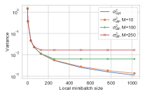
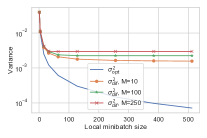
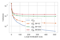
Figure 1: The effect of the dataset and number of workers $M$ on the variance parameters. Left: ‘a8a’, middle: ‘mushrooms’, right: ‘w8a’ dataset. We use uniform sampling of data points, so $\sigma_{\mathrm{opt}}^{2}$ is the same as $\sigma_{\mathrm{dif}}^{2}$ with $M=1$, while for higher values of $M$ the value of $\sigma_{\mathrm{dif}}^{2}$ might be drastically larger than $\sigma_{\mathrm{opt}}^{2}$.

Theorem 3.

Suppose that Assumptions 1 and 3 hold with $\mu>0$. Suppose that Algorithm 1 is run for identical data with $\max_{p}\left\lvert t_{p}-t_{p+1}\right\rvert\leq H$ for some $H\geq 1$ and with a stepsize $\gamma>0$ chosen such that $\gamma\leq\min\left\{\frac{1}{4L\left(1+\frac{2}{M}\right)},\frac{1}{\mu+8L\left(H-1\right)}\right\}.$ Then for any timestep $t$ such that synchronization occurs,

$$\begin{split}\mathbb{E}\left[\left\lVert\hat{x}_{t}-x_{\ast}\right\rVert^{2}\right]&\leq\left(1-\gamma\mu\right)^{t}\mathbb{E}\left[\left\lVert x_{0}-x_{\ast}\right\rVert^{2}\right]\\ &+\frac{2\gamma\sigma_{\mathrm{opt}}^{2}}{\mu M}+\frac{4\sigma_{\mathrm{opt}}^{2}\gamma^{2}\left(H-1\right)L}{\mu}.\end{split}$$ (4)

As a corollary, we can obtain an asymptotic convergence rate by choosing specific stepsizes $\gamma$ and $H$.

Corollary 3.

Let $a=18\kappa t$ for some $t>0$, let $H\leq t$ and choose $\gamma=\frac{1}{\mu a}\leq\frac{1}{9LH}$. We substitute in (4) and take $T=18a\log a$ steps, then for $r_{t}\overset{\text{def}}{=}\hat{x}_{t}-x_{\ast}$,

$$\mathbb{E}\left[\left\lVert r_{t}\right\rVert^{2}\right]=\mathcal{\tilde{O}}\Bigg{(}\frac{{\left\lVert r_{0}\right\rVert}^{2}}{T^{2}} +\frac{\sigma_{\mathrm{opt}}^{2}}{\mu^{2}MT}+\frac{\sigma_{\mathrm{opt}}^{2}\kappa(H-1)}{\mu^{2}T^{2}}\Bigg{)}.$$

Substituting $H=1+\left\lfloor t/M\right\rfloor=1+\left\lfloor T/(18\kappa M)\right\rfloor$ in Corollary 3 we get an asymptotic convergence rate of $\mathcal{\tilde{O}}\left(\frac{\sigma_{\mathrm{opt}}^{2}}{TM}\right)$. This preserves the rate of minibatch SGD up to problem-independent constants and polylogarithmic factors, but with possibly fewer communication steps.

Theorem 4.

Suppose that Assumptions 1 and 3 hold with $\mu=0$, that a stepsize $\gamma\leq\frac{1}{10LH}$ is chosen and that Algorithm 1 is run on $M\geq 2$ nodes with identical data and with $\sup_{p}\left\lvert t_{p}-t_{p+1}\right\rvert\leq H$, then for any timestep $T$ such that synchronization occurs we have for $\bar{x}_{T}=\frac{1}{T}\sum_{t=1}^{T}\hat{x}_{t}$ that

$$\begin{split}\mathbb{E}\left[f(\bar{x}_{T})-f(x_{\ast})\right]\leq&\frac{10{\left\lVert x_{0}-x_{\ast}\right\rVert}^{2}}{\gamma T}+\frac{20\gamma\sigma_{\mathrm{opt}}^{2}}{M}\\ &+40\gamma^{2}L\sigma_{\mathrm{opt}}^{2}\left(H-1\right).\end{split}$$ (5)

Corollary 4.

Let $H\leq\frac{\sqrt{T}}{\sqrt{M}}$, then for $\gamma=\frac{\sqrt{M}}{10L\sqrt{T}}$ we see that $\gamma\leq\frac{1}{10LH}$, and plugging it into (5) yields

$$\begin{split}\mathbb{E}\left[f(\bar{x}_{T})-f(x_{\ast})\right]\leq&\frac{100L{\left\lVert x_{0}-x_{\ast}\right\rVert}^{2}}{\sqrt{TM}}+\frac{2\sigma_{\mathrm{opt}}^{2}}{L\sqrt{TM}}\\ &+\frac{2\sigma_{\mathrm{opt}}^{2}M(H-1)}{5LT}.\end{split}$$

This is the same result as Corollary 2, and hence we see that choosing $H=\mathcal{O}\left(T^{1/2}M^{-3/2}\right)$ (when $T>M^{3}$) yields a linear speedup in the number of nodes $M$.

4.2 Heterogeneous Data

We next show that for arbitrarily heterogeneous convex objectives, the convergence of Local SGD is the same as Minibatch SGD plus an error that depends on $H$.

Theorem 5.

Suppose that Assumptions 1 and 3 hold with $\mu=0$ and for heterogeneous data. Then for Algorithm 1 run for different data with $M\geq 2$, $\max_{p}\left\lvert t_{p}-t_{p+1}\right\rvert\leq H$, and a stepsize $\gamma>0$ such that $\gamma\leq\min\left\{\frac{1}{4L}\frac{1}{8L(H-1)}\right\}$, then we have

$$\begin{split}\mathbb{E}\left[f(\bar{x}_{T})-f(x_{\ast})\right]\leq&\frac{4{\left\lVert r_{0}\right\rVert}^{2}}{\gamma T}+\frac{20\gamma\sigma_{\mathrm{dif}}^{2}}{M}\\ &+16\gamma^{2}L(H-1)^{2}\sigma_{\mathrm{dif}}^{2}.\end{split}$$

where $\bar{x}_{T}\overset{\text{def}}{=}\frac{1}{T}\sum_{i=0}^{T-1}\hat{x}_{i}$ and $r_{0}=x_{0}-x_{\ast}$.

Dependence on $\sigma_{\mathrm{dif}}$. We see that the convergence guarantee given by Theorem 5 shows a dependence on $\sigma_{\mathrm{dif}}$, which measures the heterogeneity of the data distribution. In typical (non-federated) distributed learning settings where data is distributed before starting training, this term can very quite significantly depending on how the data is distributed.

Dependence on $H$. We further note that the dependence on $H$ in Theorem 5 is quadratic rather than linear. This translates to a worse upper bound on the synchronization interval $H$ that still allows convergence, as the next corollary shows.

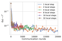
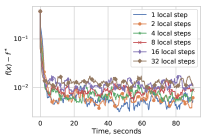
Figure 2: Results on ‘a9a’ dataset, with stepsize $\frac{1}{L}$. For any value of local iterations $H$ the method converged to a neighborhood within a small number of communication rounds due to large stepsizes.

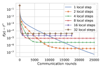
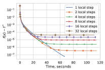
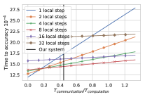
Figure 3: Convergence on heterogeneous data with different number of local steps on the ‘a5a’ dataset. 1 local step corresponds to fully synchronized gradient descent. Left: convergence in terms of communication rounds, which shows a clear advantage of local GD when only limited accuracy is required. Mid plot: wall-clock time might improve only slightly if communication is cheap. Right: what changes with different communication cost.

Corollary 5.

Choose $H\leq\frac{\sqrt{T}}{\sqrt{M}}$, then $\gamma=\frac{\sqrt{M}}{8L\sqrt{T}}\leq\frac{1}{8HL}$, and hence applying the result of Theorem 5,

$$\begin{split}\mathbb{E}\left[f(\bar{x}_{T})-f(x_{\ast})\right]\leq&\frac{32L{\left\lVert x_{0}-x_{\ast}\right\rVert}^{2}}{\sqrt{MT}}\\ &+\frac{5\sigma_{\mathrm{dif}}^{2}}{2L\sqrt{MT}}+\frac{\sigma_{\mathrm{dif}}^{2}M(H-1)^{2}}{4LT}.\end{split}$$

Optimal $H$. By Corollary 5 we see that the optimal value of $H$ is $H=1+\left\lfloor T^{1/4}M^{-3/4}\right\rfloor$, which gives $\mathcal{O}\left(\frac{1}{\sqrt{MT}}\right)$ convergence rate. Thus, the same convergence rate is attained provided that communication is more frequent compared to the identical data regime.

5 Experiments

All experiments described below were run on logistic regression problem with $\ell_{2}$ regularization of order $\frac{1}{n}$. The datasets were taken from the LIBSVM library [Chang and Lin, 2011]. The code was written in Python using MPI [Dalcin et al., 2011] and run on Intel(R) Xeon(R) Gold 6146 CPU @3.20GHz cores in parallel.

5.1 Variance measures

We provide values of $\sigma_{\mathrm{dif}}^{2}$ and $\sigma_{\mathrm{opt}}^{2}$ in Figure 1 for different datasets, minibatch sizes and $M$. The datasets were split evenly without any data reshuffling and no overlaps. For any $M>1$, the value of $\sigma_{\mathrm{dif}}$ is lower bounded by $\frac{1}{M}\sum_{m=1}^{M}\parallel\nabla f_{m}(x_{*})\parallel^{2}$ which explains the difference between identical and heterogeneous data.

5.2 Identical Data

For identical data we used $M=20$ nodes and ’a9a’ dataset. We estimated $L$ numerically and ran two experiments, with stepsizes $\frac{1}{L}$ and $\frac{0.05}{L}$ and minibatch size equal 1. In both cases we observe convergence to a neighborhood, although of a different radius. Since we run the experiments on a single machine, the communication is very cheap and there is little gain in time required for convergence. However, the advantage in terms of required communication rounds is self-evident and can lead to significant time improvement under slow communication networks. The results are provided here in Figure 2 and in the supplementary material in Figure 5.

5.3 Heterogeneous Data

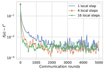
Figure 4: Convergence of local SGD on heterogeneous data with different number of local steps on the ‘a5a’ dataset.

Since our architecture leads to a very specific trade-off between computation and communication, we provide plots for the case the communication time relative to gradient computation time is higher or lower. To see the impact of $\sigma_{\mathrm{dif}}$, in all experiments we use full gradients $\nabla f_{m}$ and constant stepsize $\frac{1}{L}$. The data partitioning is not i.i.d. and is done based on the index in the original dataset. The results are provided in Figure 3 and in the supplementary material in Figure 6. In cases where communication is significantly more expensive than gradient computation, local methods are much faster for imprecise convergence.

6 Acknowledgments

We thank Li Yipeng for spotting multiple typos in the paper.

Supplementary Material

Contents

1. 1 Introduction
2. 2 Related Work
   1. 2.1 Local SGD with Identical Data
   2. 2.2 Local SGD with Heterogeneous Data
3. 3 Settings and Contributions
4. 4 Convergence Theory
   1. 4.1 Identical Data
   2. 4.2 Heterogeneous Data
5. 5 Experiments
   1. 5.1 Variance measures
   2. 5.2 Identical Data
   3. 5.3 Heterogeneous Data
6. 6 Acknowledgments
7. 7 Basic Facts and Notation
8. 8 Proofs for Identical data under Assumption 2
   1. 8.1 Proof of Lemma 1
   2. 8.2 Two More Lemmas
   3. 8.3 Proof of Theorem 1
   4. 8.4 Proof of Theorem 2
9. 9 Proofs for identical data under Assumption 3
   1. 9.1 Preliminary Lemmas
   2. 9.2 Proof of Theorem 3
   3. 9.3 Proof of Theorem 4
10. 10 Proofs for Heterogeneous data
    1. 10.1 Preliminary Lemmas
    2. 10.2 Proof of Theorem 5
11. 11 Extra Experiments
12. 12 Discussion of Dieuleveut and Patel (2019)

7 Basic Facts and Notation

We use a notation similar to that of Stich [2019] and denote the sequence of time stamps when synchronization happens as $(t_{p})_{p=1}^{\infty}$. Given stochastic gradients $g_{t}^{1},g_{t}^{2},\ldots,g_{t}^{M}$ at time $t\geq 0$ we define

$$g_{t}\overset{\text{def}}{=}\frac{1}{M}\sum_{m=1}^{M}g_{t}^{m}, \bar{g}_{t}^{m}\overset{\text{def}}{=}\mathbb{E}\left[g_{t}^{m}\right]=\begin{cases}\nabla f(x_{t}^{m})&\text{ for identical data }\\ \nabla f_{m}(x_{t}^{m})&\text{ otherwise. }\end{cases} \bar{g}_{t}\overset{\text{def}}{=}\mathbb{E}\left[g_{t}\right].$$

We define an epoch to be a sequence of timesteps between two synchronizations: for $p\in\mathbb{N}$ an epoch is the sequence $t_{t_{p}},t_{t_{p}+1},\ldots,t_{t_{p+1}-1}$. We summarize some of the notation used in Table 3.

Table 3: Common Notation Summary.

Symbol	Description
$g_{t}^{m}$	Stochastic gradient at time $t$ on node $m$. See Algorithm 1.
$x_{t}^{m}$	Local iterate at time $t$ on node $m$. See Algorithm 1.
$g_{t}$	Average of stochastic gradients across nodes at time $t$. See Algorithm 1.
$\bar{g}_{t}$	Expected value of $g_{t}$: $\mathbb{E}\left[g_{t}\right]=\bar{g}_{t}$.
$\hat{x}_{t}$	The average of all local iterates at time $t$.
$r_{t}$	The deviation of the average iterate from the optimum $\hat{x}_{t}-x_{\ast}$ at time $t$.
$\sigma^{2}$	Uniform bound on the variance of the stochastic gradients for identical data. See Assumption 2.
$\sigma_{\mathrm{opt}}^{2}$	The variance of the stochastic gradients at the optimum for identical data. See Assumption 3.
$\sigma_{\mathrm{dif}}^{2}$	The variance of the stochastic gradients at the optimum for heterogeneous data. See Assumption 3.
$t_{1},t_{2},\ldots,t_{p}$	Timesteps at which synchronization happen in Algorithm 1.
$H$	Upper bound on the maximum number of local computations between timesteps, i.e. $\max_{p}\left\lvert t_{p}-t_{p+1}\right\rvert\leq H$.

Throughout the proofs, we will use the variance decomposition that holds for any random vector $X$ with finite second moment:

$$\mathbb{E}\left[\left\lVert X\right\rVert^{2}\right]=\mathbb{E}\left[\left\lVert X-\mathbb{E}\left[X\right]\right\rVert^{2}\right]+{\left\lVert\mathbb{E}\left[X\right]\right\rVert}^{2}.$$ (6)

In particular, its version for vectors with finite number of values gives

$$\frac{1}{M}\sum_{m=1}^{M}\left\lVert X_{m}\right\rVert^{2}=\frac{1}{M}\sum_{m=1}^{M}\left\lVert X_{m}-\frac{1}{M}\sum_{i=1}^{M}X_{i}\right\rVert^{2}+\left\lVert\frac{1}{M}\sum_{m=1}^{M}X_{m}\right\rVert^{2}.$$ (7)

As a consequence of (6) we have that,

$$\mathbb{E}\left[\left\lVert X-\mathbb{E}\left[X\right]\right\rVert^{2}\right]\leq\mathbb{E}\left[\left\lVert X\right\rVert^{2}\right].$$ (8)

Proposition 1 (Jensen’s inequality).

For any convex function $f$ and any vectors $x^{1},\dotsc,x^{M}$ we have

$$f\left(\frac{1}{M}\sum_{m=1}^{M}x^{m}\right)\leq\frac{1}{M}\sum_{m=1}^{M}f(x^{m}).$$ (9)

As a special case with $f(x)=\parallel x\parallel^{2}$, we obtain

$$\left\lVert\frac{1}{M}\sum_{m=1}^{M}x_{m}\right\rVert^{2}\leq\frac{1}{M}\sum_{m=1}^{M}\parallel x_{m}\parallel^{2}.$$ (10)

We denote the Bregman divergence associated with function $f$ and arbitrary $x,y$ as

$$D_{f}(x,y)\overset{\text{def}}{=}f(x)-f(y)-\left\langle\nabla f(y),x-y\right\rangle.$$

Proposition 2.

If $f$ is $L$-smooth and convex, then for any $x$ and $y$ it holds

$$\parallel\nabla f(x)-\nabla f(y)\parallel^{2}\leq 2LD_{f}(x,y).$$ (11)

If $f$ satisfies Assumption 1, then

$$f(x)+\left\langle\nabla f(y),x-y\right\rangle+\frac{\mu}{2}{\left\lVert y-x\right\rVert}^{2}\leq f(y)\qquad\forall x,y\in\mathbb{R}^{d}.$$ (12)

We will also use the following facts from linear algebra:

$${\left\lVert x+y\right\rVert}^{2} \leq 2{\left\lVert x\right\rVert}^{2}+2{\left\lVert y\right\rVert}^{2},$$ (13)

$$2\left\langle a,b\right\rangle \leq\zeta{\left\lVert a\right\rVert}^{2}+\zeta^{-1}{\left\lVert b\right\rVert}^{2}\text{ for all }a,b\in\mathbb{R}^{d}\text{ and }\zeta>0.$$ (14)

8 Proofs for Identical data under Assumption 2

8.1 Proof of Lemma 1

Proof.

Let $t\in\mathbb{N}$ be such that $t_{p}\leq t\leq t_{p+1}-1$. Recall that for a time $t$ such that $t_{p}\leq t<t_{p+1}$ we have $x_{t+1}^{m}=x_{t}^{m}-\gamma g_{t}^{m}$ and $\hat{x}_{t+1}=\hat{x}_{t}-\gamma g_{t}$. Hence for the expectation conditional on $x_{t}^{1},x_{t}^{2},\ldots,x_{t}^{M}$ we have:

$$\mathbb{E}\left[\left\lVert x_{t+1}^{m}-\hat{x}_{t+1}\right\rVert^{2}\right] ={\left\lVert x_{t}^{m}-\hat{x}_{t}\right\rVert}^{2}+\gamma^{2}\mathbb{E}\left[\left\lVert g_{t}^{m}-g_{t}\right\rVert^{2}\right]-2\gamma\mathbb{E}\left[\left\langle x_{t}^{m}-\hat{x}_{t},g_{t}^{m}-g_{t}\right\rangle\right]$$

$$={\left\lVert x_{t}^{m}-\hat{x}_{t}\right\rVert}^{2}+\gamma^{2}\mathbb{E}\left[\left\lVert g_{t}^{m}-g_{t}\right\rVert^{2}\right]-2\gamma\left\langle x_{t}^{m}-\hat{x}_{t},\nabla f(x_{t}^{m})\right\rangle$$

$$\quad+2\gamma\left\langle x_{t}^{m}-\hat{x}_{t},\bar{g}_{t}\right\rangle.$$

Averaging both sides and letting $V_{t}=\frac{1}{M}\sum_{m}{\left\lVert x_{t}^{m}-\hat{x}_{t}\right\rVert}^{2}$, we have

$$\mathbb{E}\left[V_{t+1}\right] =V_{t}+\frac{\gamma^{2}}{M}\sum_{m}\mathbb{E}\left[\left\lVert g_{t}^{m}-g_{t}\right\rVert^{2}\right]-\frac{2\gamma}{M}\sum_{m}\left\langle x_{t}^{m}-\hat{x}_{t},\nabla f(x_{t}^{m})\right\rangle+2\gamma\underbrace{\left\langle\hat{x}_{t}-\hat{x}_{t},\bar{g}_{t}\right\rangle}_{=0}$$

$$=V_{t}+\frac{\gamma^{2}}{M}\sum_{m}\mathbb{E}\left[\left\lVert g_{t}^{m}-g_{t}\right\rVert^{2}\right]-\frac{2\gamma}{M}\sum_{m}\left\langle x_{t}^{m}-\hat{x}_{t},\nabla f(x_{t}^{m})\right\rangle.$$ (15)

Now note that by expanding the square we have,

$$\mathbb{E}\left[\left\lVert g_{t}^{m}-g_{t}\right\rVert^{2}\right] =\mathbb{E}\left[\left\lVert g_{t}^{m}-\bar{g_{t}}\right\rVert^{2}\right]+\mathbb{E}\left[\left\lVert\bar{g}_{t}-g_{t}\right\rVert^{2}\right]+2\mathbb{E}\left[\left\langle g_{t}^{m}-\bar{g}_{t},\bar{g}_{t}-g_{t}\right\rangle\right].$$ (16)

We decompose the first term in the last equality again by expanding the square,

$$\mathbb{E}\left[\left\lVert g_{t}^{m}-\bar{g}_{t}\right\rVert^{2}\right] =\mathbb{E}\left[\left\lVert g_{t}^{m}-\bar{g}_{t}^{m}\right\rVert^{2}\right]+{\left\lVert\bar{g}_{t}^{m}-\bar{g}_{t}\right\rVert}^{2}+2\mathbb{E}\left[\left\langle g_{t}^{m}-\bar{g}_{t}^{m},\bar{g}_{t}^{m}-\bar{g}_{t}\right\rangle\right]$$

$$=\mathbb{E}\left[\left\lVert g_{t}^{m}-\bar{g}_{t}^{m}\right\rVert^{2}\right]+{\left\lVert\bar{g}_{t}^{m}-\bar{g}_{t}\right\rVert}^{2}+2\underbrace{\left\langle\bar{g}_{t}^{m}-\bar{g}_{t}^{m},\bar{g}_{t}^{m}-\bar{g}_{t}\right\rangle}_{=0}$$

$$=\mathbb{E}\left[\left\lVert g_{t}^{m}-\bar{g}_{t}^{m}\right\rVert^{2}\right]+{\left\lVert\bar{g}_{t}^{m}-\bar{g}_{t}\right\rVert}^{2}.$$

Plugging this into (16) we have,

$$\mathbb{E}\left[\left\lVert g_{t}^{m}-g_{t}\right\rVert^{2}\right] =\mathbb{E}\left[\left\lVert g_{t}^{m}-\bar{g}_{t}^{m}\right\rVert^{2}\right]+{\left\lVert\bar{g}_{t}^{m}-\bar{g}_{t}\right\rVert}^{2}+\mathbb{E}\left[\left\lVert\bar{g}_{t}-g_{t}\right\rVert^{2}\right]+2\mathbb{E}\left[\left\langle g_{t}^{m}-\bar{g}_{t},\bar{g}_{t}-g_{t}\right\rangle\right].$$

Now average over $m$:

$$\frac{1}{M}\sum_{m}\mathbb{E}\left[\left\lVert g_{t}^{m}-g_{t}\right\rVert^{2}\right] =\frac{1}{M}\sum_{m}\mathbb{E}\left[\left\lVert g_{t}^{m}-\bar{g}_{t}^{m}\right\rVert^{2}\right]+\frac{1}{M}\sum_{m}{\left\lVert\bar{g}_{t}^{m}-\bar{g}_{t}\right\rVert}^{2}+\mathbb{E}\left[\left\lVert\bar{g}_{t}-g_{t}\right\rVert^{2}\right]$$

$$-2\mathbb{E}\left[\left\lVert\bar{g}_{t}-g_{t}\right\rVert^{2}\right],$$

where we used that by definition $\frac{1}{M}\sum_{m=1}^{M}g_{t}^{m}=g_{t}$. Hence,

$$\frac{1}{M}\sum_{m}\mathbb{E}\left[\left\lVert g_{t}^{m}-g_{t}\right\rVert^{2}\right] =\frac{1}{M}\sum_{m}\mathbb{E}\left[\left\lVert g_{t}^{m}-\bar{g}_{t}^{m}\right\rVert^{2}\right]+\frac{1}{M}\sum_{m}{\left\lVert\bar{g}_{t}^{m}-\bar{g}_{t}\right\rVert}^{2}-\mathbb{E}\left[\left\lVert\bar{g}_{t}-g_{t}\right\rVert^{2}\right]$$

$$\leq\frac{1}{M}\sum_{m}\mathbb{E}\left[\left\lVert g_{t}^{m}-\bar{g}_{t}^{m}\right\rVert^{2}\right]+\frac{1}{M}\sum_{m}{\left\lVert\bar{g}_{t}^{m}-\bar{g}_{t}\right\rVert}^{2}.$$ (17)

Now note that for the first term in (17) we have by Assumption 2,

$$\mathbb{E}\left[\left\lVert g_{t}^{m}-\bar{g}_{t}^{m}\right\rVert^{2}\right] =\mathbb{E}\left[\left\lVert g_{t}^{m}-\nabla f(x_{t}^{m})\right\rVert^{2}\right]\leq\sigma^{2}.$$ (18)

For the second term in (17) we have

$${\left\lVert\bar{g}_{t}^{m}-\bar{g}_{t}\right\rVert}^{2} ={\left\lVert\bar{g}_{t}^{m}-\nabla f(\hat{x}_{t})\right\rVert}^{2}+{\left\lVert\nabla f(\hat{x}_{t})-\bar{g}_{t}\right\rVert}^{2}+2\left\langle\bar{g}_{t}^{m}-\nabla f(\hat{x}_{t}),\nabla f(\hat{x}_{t})-\bar{g}_{t}\right\rangle.$$

Averaging over $m$,

$$\frac{1}{M}\sum_{m=1}^{M}{\left\lVert\bar{g}_{t}^{m}-\bar{g}_{t}\right\rVert}^{2} =\frac{1}{M}\sum_{m}{\left\lVert\bar{g}_{t}^{m}-\nabla f(\hat{x}_{t})\right\rVert}^{2}+{\left\lVert\nabla f(\hat{x}_{t})-\bar{g}_{t}\right\rVert}^{2}+2\left\langle\bar{g}_{t}-\nabla f(\hat{x}_{t}),\nabla f(\hat{x}_{t})-\bar{g}_{t}\right\rangle$$

$$=\frac{1}{M}\sum_{m}{\left\lVert\bar{g}_{t}^{m}-\nabla f(\hat{x}_{t})\right\rVert}^{2}+{\left\lVert\nabla f(\hat{x}_{t})-\bar{g}_{t}\right\rVert}^{2}-2{\left\lVert\nabla f(\hat{x}_{t})-\bar{g}_{t}\right\rVert}^{2}$$

$$=\frac{1}{M}\sum_{m}{\left\lVert\bar{g}_{t}^{m}-\nabla f(\hat{x}_{t})\right\rVert}^{2}-{\left\lVert\nabla f(\hat{x}_{t})-\bar{g}_{t}\right\rVert}^{2}\leq\frac{1}{M}\sum_{m}{\left\lVert\bar{g}_{t}^{m}-\nabla f(\hat{x}_{t})\right\rVert}^{2},$$

where we used the fact that $\frac{1}{M}\sum_{m}\bar{g}_{t}^{m}=\bar{g}_{t}$, which comes from the linearity of expectation. Now we bound ${\left\lVert\bar{g}_{t}^{m}-\nabla f(\hat{x}_{t})\right\rVert}^{2}$ in the last inequality by smoothness and then use that Jensen’s inequality implies $\sum_{m=1}^{M}(f(\hat{x}_{t})-f(x_{t}^{m}))\leq 0$,

$$\frac{1}{M}\sum_{m}{\left\lVert\bar{g}_{t}^{m}-\nabla f(\hat{x}_{t})\right\rVert}^{2} =\frac{1}{M}\sum_{m}{\left\lVert\nabla f(x_{t}^{m})-\nabla f(\hat{x}_{t})\right\rVert}^{2}$$

$$\overset{\eqref{eq:bregman-dif}}{\leq}\frac{1}{M}\sum_{m}2L(f(\hat{x}_{t})-f(x_{t}^{m})-\left\langle\hat{x}_{t}-x_{t}^{m},\nabla f(x_{t}^{m})\right\rangle)$$

$$\leq\frac{2L}{M}\sum_{m}\left\langle x_{t}^{m}-\hat{x}_{t},\nabla f(x_{t}^{m})\right\rangle.$$ (19)

Plugging in (19) and (18) into (17) we have,

$$\frac{1}{M}\sum_{m}\mathbb{E}\left[\left\lVert g_{t}^{m}-g_{t}\right\rVert^{2}\right]\leq\sigma^{2}+\frac{2L}{M}\sum_{m}\left\langle x_{t}^{m}-\hat{x}_{t},\nabla f(x_{t}^{m})\right\rangle.$$ (20)

Plugging (20) into (15), we get

$$\mathbb{E}\left[V_{t+1}\right] \leq V_{t}+\gamma^{2}\sigma^{2}-\frac{2\gamma}{M}\sum_{m}\left\langle x_{t}^{m}-\hat{x}_{t},\nabla f(x_{t}^{m})\right\rangle+\frac{2L\gamma^{2}}{M}\sum_{m}\left\langle x_{t}^{m}-\hat{x}_{t},\nabla f(x_{t}^{m})\right\rangle$$

$$=V_{t}+\gamma^{2}\sigma^{2}-\frac{2\gamma(1-\gamma L)}{M}\sum_{m}\left\langle x_{t}^{m}-\hat{x}_{t},\nabla f(x_{t}^{m})\right\rangle$$ (21)

$$\overset{\eqref{eq:asm-strong-convexity}}{\leq}\left(1-\gamma(1-\gamma L)\mu\right)V_{t}+\gamma^{2}\sigma^{2}.$$

Using that $\gamma\leq\frac{1}{2L}$ we can conclude,

$$\mathbb{E}\left[V_{t+1}\right] \leq\left(1-\frac{\gamma\mu}{2}\right)V_{t}+\gamma^{2}\sigma^{2}$$

$$\leq V_{t}+\gamma^{2}\sigma^{2}.$$

Taking expectations and iterating the above inequality,

$$\mathbb{E}\left[V_{t}\right] \leq\mathbb{E}\left[V_{t_{p}}\right]+\gamma^{2}\sigma^{2}\left(t-t_{p}\right)$$

$$\leq\mathbb{E}\left[V_{t_{p}}\right]+\gamma^{2}\sigma^{2}\left(t_{p+1}-t_{p}-1\right)$$

$$\leq\mathbb{E}\left[V_{t_{p}}\right]+\gamma^{2}\sigma^{2}\left(H-1\right).$$

It remains to notice that by assumption we have $V_{t_{p}}=0$. ∎

8.2 Two More Lemmas

Lemma 2.

[Stich, 2019]. Let $(x_{t}^{m})_{t\geq 0}$ be iterates generated by Algorithm 1 run with identical data. Suppose that $f$ satisfies Assumption 1 and that $\gamma\leq\frac{1}{2L}$. Then,

$$\begin{split}\mathbb{E}\left[\left\lVert\hat{x}_{t+1}-x_{\ast}\right\rVert^{2}\right]\leq(1&-\gamma\mu)\mathbb{E}\left[\left\lVert\hat{x}_{t}-x_{\ast}\right\rVert^{2}\right]+\gamma^{2}\mathbb{E}\left[\left\lVert g_{t}-\bar{g}_{t}\right\rVert^{2}\right]\\ &-\frac{\gamma}{2}\mathbb{E}\left[D_{f}(\hat{x}_{t},x_{\ast})\right]+2\gamma L\mathbb{E}\left[V_{t}\right].\end{split}$$ (22)

Proof.

This is Lemma 3.1 in [Stich, 2019]. ∎

Lemma 3.

Suppose that Assumption 2 holds. Then,

$$\mathbb{E}\left[\left\lVert g_{t}-\bar{g}_{t}\right\rVert^{2}\right]\leq\frac{\sigma^{2}}{M}.$$

Proof.

This is Lemma 3.2 in [Stich, 2019]. Because the stochastic gradients $g_{t}^{m}$ are independent we have that the variance of their sum is the sum of their variances, hence

$$\mathbb{E}\left[\left\lVert g_{t}-\bar{g}_{t}\right\rVert^{2}\right] =\frac{1}{M^{2}}\mathbb{E}\left[\left\lVert\sum_{m=1}^{M}g_{t}^{m}-\bar{g}_{t}^{m}\right\rVert^{2}\right]=\frac{1}{M^{2}}\sum_{m=1}^{M}\mathbb{E}\left[\left\lVert g_{t}^{m}-\bar{g}_{t}^{m}\right\rVert^{2}\right]\leq\frac{\sigma^{2}}{M}.$$

∎

8.3 Proof of Theorem 1

Proof.

Combining Lemma 2 and Lemma 3, we have

$$\mathbb{E}\left[\left\lVert\hat{x}_{t+1}-x_{\ast}\right\rVert^{2}\right]\leq(1-\gamma\mu)\mathbb{E}\left[\left\lVert\hat{x}_{t}-x_{\ast}\right\rVert^{2}\right]+\frac{\gamma^{2}\sigma^{2}}{M}-\frac{\gamma}{2}\mathbb{E}\left[D_{f}(\hat{x}_{t},x_{\ast})\right]+2\gamma L\mathbb{E}\left[V_{t}\right].$$ (23)

Using Lemma 1 we can upper bound the $\mathbb{E}\left[V_{t}\right]$ term in $\eqref{sc-thm-proof-1}$:

$$\mathbb{E}\left[\left\lVert\hat{x}_{t+1}-x_{\ast}\right\rVert^{2}\right]\leq(1-\gamma\mu)\mathbb{E}\left[\left\lVert\hat{x}_{t}-x_{\ast}\right\rVert^{2}\right]+\frac{\gamma^{2}\sigma^{2}}{M}-\frac{\gamma}{2}\mathbb{E}\left[D_{f}(\hat{x}_{t},x_{\ast})\right]+2\gamma^{3}L\left(H-1\right)\sigma^{2}.$$

Letting $r_{t+1}=\hat{x}_{t+1}-x_{\ast}$ and we have,

$$\mathbb{E}\left[\left\lVert r_{t+1}\right\rVert^{2}\right]\leq\left(1-\gamma\mu\right)\mathbb{E}\left[\left\lVert r_{t}\right\rVert^{2}\right]+\frac{\gamma^{2}\sigma^{2}}{M}+2\gamma^{3}L\left(H-1\right)\sigma^{2}.$$

Recursing the above inequality we have,

$$\mathbb{E}\left[\left\lVert r_{T}\right\rVert^{2}\right]\leq\left(1-\gamma\mu\right)^{T}\mathbb{E}\left[\left\lVert r_{0}\right\rVert^{2}\right]+\left(\sum_{t=0}^{T-1}\left(1-\gamma\mu\right)^{t}\right)\left(\frac{\gamma^{2}\sigma^{2}}{M}+2\gamma^{3}L\left(H-1\right)\sigma^{2}\right).$$

Using that $\sum_{t=0}^{T-1}\left(1-\gamma\mu\right)^{t}\leq\sum_{t=0}^{\infty}\left(1-\gamma\mu\right)^{t}=\frac{1}{\gamma\mu}$ we have,

$$\mathbb{E}\left[\left\lVert r_{T}\right\rVert^{2}\right]\leq\left(1-\gamma\mu\right)^{T}\mathbb{E}\left[\left\lVert r_{0}\right\rVert^{2}\right]+\frac{\gamma\sigma^{2}}{\mu M}+\frac{2\gamma^{2}L\left(H-1\right)\sigma^{2}}{\mu},$$

which is the claim of this theorem. ∎

8.4 Proof of Theorem 2

Proof.

Let $r_{t}=\hat{x}_{t}-x_{\ast}$, then putting $\mu=0$ in Lemma 2 and combining it with Lemma 3, we have

$$\mathbb{E}\left[\left\lVert r_{t+1}\right\rVert^{2}\right]\leq\mathbb{E}\left[\left\lVert r_{t}\right\rVert^{2}\right]+\frac{\gamma^{2}\sigma^{2}}{M}-\frac{\gamma}{2}\mathbb{E}\left[D_{f}(\hat{x}_{t},x_{\ast})\right]+2\gamma L\mathbb{E}\left[V_{t}\right].$$

Further using Lemma 1,

$$\mathbb{E}\left[\left\lVert r_{t+1}\right\rVert^{2}\right]\leq\mathbb{E}\left[\left\lVert r_{t}\right\rVert^{2}\right]+\frac{\gamma^{2}\sigma^{2}}{M}-\frac{\gamma}{2}\mathbb{E}\left[D_{f}(\hat{x}_{t},x_{\ast})\right]+2\gamma^{3}L\left(H-1\right)\sigma^{2}.$$

Rearranging we have,

$$\frac{\gamma}{2}\mathbb{E}\left[D_{f}(\hat{x}_{t},x_{\ast})\right]\leq\mathbb{E}\left[\left\lVert r_{t}\right\rVert^{2}\right]-\mathbb{E}\left[\left\lVert r_{t+1}\right\rVert^{2}\right]+\frac{\gamma^{2}\sigma^{2}}{M}+2\gamma^{3}L\left(H-1\right)\sigma^{2}.$$

Averaging the above equation as $t$ varies between $0$ and $T-1$,

$$\frac{\gamma}{2T}\sum_{t=0}^{T-1}\mathbb{E}\left[D_{f}(\hat{x}_{t},x_{\ast})\right] \leq\frac{1}{T}\sum_{t=0}^{T-1}\mathbb{E}\left[\left\lVert r_{t}\right\rVert^{2}\right]-\mathbb{E}\left[\left\lVert r_{t+1}\right\rVert^{2}\right]+\frac{1}{T}\sum_{t=0}^{T-1}\left(\frac{\gamma^{2}\sigma^{2}}{M}+2\gamma^{3}L\left(H-1\right)\sigma^{2}\right)$$

$$=\frac{{\left\lVert r_{0}\right\rVert}^{2}-\mathbb{E}\left[\left\lVert r_{T}\right\rVert^{2}\right]}{T}+\frac{\gamma^{2}\sigma^{2}}{M}+2\gamma^{3}L\left(H-1\right)\sigma^{2}$$

$$\leq\frac{{\left\lVert r_{0}\right\rVert}^{2}}{T}+\frac{\gamma^{2}\sigma^{2}}{M}+2\gamma^{3}L\left(H-1\right)\sigma^{2}.$$ (24)

By Jensen’s inequality we have $D_{f}(\bar{x}_{T},x_{\ast})\leq\frac{1}{T}\sum_{t=0}^{T-1}D_{f}(\hat{x}_{t},x_{\ast})$. Using this in (24) we have,

$$\frac{\gamma}{2}\mathbb{E}\left[D_{f}(\hat{x}_{t},x_{\ast})\right]\leq\frac{{\left\lVert r_{0}\right\rVert}^{2}}{T}+\frac{\gamma^{2}\sigma^{2}}{M}+2\gamma^{3}L\left(H-1\right)\sigma^{2}.$$

Dividing both sides by $\gamma/2$ yields the theorem’s claim. ∎

9 Proofs for identical data under Assumption 3

9.1 Preliminary Lemmas

Lemma 4.

Individual gradient variance bound: assume that Assumption 3 holds with identical data, then for all $t\geq 0$ and $m\in[M]$ we have

$$\mathbb{E}\left[\left\lVert g_{t}^{m}\right\rVert^{2}\right]\leq 4LD_{f}(x_{t}^{m},x_{\ast})+2\sigma_{m}^{2},$$ (25)

where $\sigma_{m}^{2}\overset{\text{def}}{=}\mathbb{E}_{z_{m}\sim\mathcal{D}_{m}}\left[\left\lVert\nabla f(x_{\ast},z_{m})\right\rVert^{2}\right]$ is the noise at the optimum on the $m$-th node.

Proof.

Using that $g_{t}^{m}=\nabla f(x_{t}^{m},z_{m})$ for some $z_{m}\sim\mathcal{D}_{m}$,

$${\left\lVert g_{t}^{m}\right\rVert}^{2} ={\left\lVert\nabla f(x_{t}^{m},z_{m})\right\rVert}^{2}$$

$$\overset{\eqref{eq:sum_sqnorm}}{\leq}2{\left\lVert\nabla f(x_{t}^{m},z_{m})-\nabla f(x_{\ast},z_{m})\right\rVert}^{2}+2{\left\lVert\nabla f(x_{\ast},z_{m})\right\rVert}^{2}$$

$$\overset{\eqref{eq:bregman-dif}}{\leq}4L\left(f(x_{t}^{m},z_{m})-f(x_{\ast},z_{m})-\left\langle\nabla f(x_{\ast},z_{m}),x_{t}^{m}-x_{\ast}\right\rangle\right)+2{\left\lVert\nabla f(x_{\ast},z_{m})\right\rVert}^{2}.$$

Taking expectations and using that $\mathbb{E}\left[\nabla f(x_{\ast},z)\right]=\nabla f(x_{\ast})=0$ we get,

$$\mathbb{E}\left[\left\lVert g_{t}^{m}\right\rVert^{2}\right] \leq 4L\left(f(x_{t}^{m})-f(x_{\ast})\right)+2\sigma_{m}^{2}$$

$$=4LD_{f}(x_{t}^{m},x_{\ast})+2\sigma_{m}^{2}.$$

∎

Lemma 5 (Average gradient variance reduction).

Assume that Assumption 3 holds with identical data, then for all $t\geq 0$ and for $M$ nodes we have,

$$\mathbb{E}\left[\left\lVert g_{t}-\bar{g}_{t}\right\rVert^{2}\right]\leq\frac{2\sigma_{\mathrm{opt}}^{2}}{M}+\frac{4L}{M^{2}}\sum_{m=1}^{M}D_{f}(x_{t}^{m},x_{\ast}).$$ (26)

Proof.

Using the definition of $g_{t}$ and $\bar{g}_{t}$,

$$\mathbb{E}\left[\left\lVert g_{t}-\bar{g}_{t}\right\rVert^{2}\right] =\mathbb{E}\left[\left\lVert\frac{1}{M}\sum_{m=1}^{M}g_{t}^{m}-\nabla f(x_{t}^{m})\right\rVert^{2}\right]$$

$$=\frac{1}{M^{2}}\mathbb{E}\left[\left\lVert\sum_{m=1}^{M}\left(g_{t}^{m}-\nabla f(x_{t}^{m})\right)\right\rVert^{2}\right].$$ (27)

The sum in (27) is the variance of a sum of independent random variables and hence can be decomposed into the sum of their individual variances which we can use Lemma 4 to bound:

$$\mathbb{E}\left[\left\lVert g_{t}-\bar{g}_{t}\right\rVert^{2}\right] =\frac{1}{M^{2}}\sum_{m=1}^{M}\mathbb{E}\left[\left\lVert g_{t}^{m}-\nabla f(x_{t}^{m})\right\rVert^{2}\right]$$

$$\overset{\eqref{eq:variance_sqnorm_upperbound}}{\leq}\frac{1}{M^{2}}\sum_{m=1}^{M}\mathbb{E}\left[\left\lVert g_{t}^{m}\right\rVert^{2}\right]$$

$$\overset{\eqref{eq:lma-gradient-smoothness-bound}}{\leq}\frac{1}{M^{2}}\sum_{m=1}^{M}\left(2\sigma_{m}^{2}+4LD_{f}(x_{t}^{m},x_{\ast})\right)$$

$$=\frac{2\sigma_{\mathrm{opt}}^{2}}{M}+\frac{4L}{M^{2}}\sum_{m=1}^{M}D_{f}(x_{t}^{m},x_{\ast}),$$

where in the last equality we used that $\sigma_{\mathrm{opt}}^{2}$ is by definition equal to $\sum_{m=1}^{M}\sigma_{m}^{2}/M$. ∎

Lemma 6.

Perturbed iterate analysis: this bounds the optimality gap across one iteration when the descent step is $\hat{x}_{t+1}=\hat{x}_{t}-\frac{\gamma}{M}\sum_{m=1}^{M}\nabla f(x_{t}^{m})$, i.e. when the expectation of the local SGD update is used. Suppose that Assumptions 1, and 3 hold with identical data. Then,

$$\begin{split}{\left\lVert\hat{x}_{t+1}-\gamma\bar{g}_{t}-x_{\ast}\right\rVert}^{2}\leq{\left\lVert\hat{x}_{t}-x_{\ast}\right\rVert}^{2}&+2\gamma LV_{t}\\ &+\frac{2\gamma}{M}\sum_{m=1}^{M}\left(\left(\gamma L-\frac{1}{2}\right)\left(f(x_{t}^{m})-f(x_{\ast})\right)-\frac{\mu}{2}{\left\lVert x_{t}^{m}-x_{\ast}\right\rVert}^{2}\right).\end{split}$$ (28)

Proof.

This is the first part of Lemma 3.1 in [Stich, 2019] and we reproduce it for completeness:

$${\left\lVert\hat{x}_{t}-x_{\ast}-\gamma\bar{g}_{t}\right\rVert}^{2}={\left\lVert\hat{x}_{t}-x_{\ast}\right\rVert}^{2} +\gamma^{2}{\left\lVert\bar{g}_{t}\right\rVert}^{2}-2\gamma\left\langle\hat{x}_{t}-x_{\ast},\bar{g}_{t}\right\rangle$$

$$={\left\lVert\hat{x}_{t}-x_{\ast}\right\rVert}^{2} +\gamma^{2}{\left\lVert\bar{g}_{t}\right\rVert}^{2}-\frac{2\gamma}{M}\sum_{m=1}^{M}\left\langle\hat{x}_{t}-x_{\ast},\nabla f(x_{t}^{m})\right\rangle$$

$$\overset{\eqref{eq:jensen_norm}}{\leq}{\left\lVert\hat{x}_{t}-x_{\ast}\right\rVert}^{2} +\frac{\gamma^{2}}{M}\sum_{m=1}^{M}{\left\lVert\nabla f(x_{t}^{m})\right\rVert}^{2}-\frac{2\gamma}{M}\sum_{m=1}^{M}\left\langle\hat{x}_{t}-x_{t}^{m}+x_{t}^{m}-x_{\ast},\nabla f(x_{t}^{m})\right\rangle$$

$$\begin{split}={\left\lVert\hat{x}_{t}-x_{\ast}\right\rVert}^{2}&+\frac{\gamma^{2}}{M}\sum_{m=1}^{M}{\left\lVert\nabla f(x_{t}^{m})-f(x_{\ast})\right\rVert}^{2}-\frac{2\gamma}{M}\sum_{m=1}^{M}\left\langle x_{t}^{m}-x_{\ast},\nabla f(x_{t}^{m})\right\rangle\\ &-\frac{2\gamma}{M}\sum_{m=1}^{M}\left\langle\hat{x}_{t}-x_{t}^{m},\nabla f(x_{t}^{m})\right\rangle\end{split}$$

$$\begin{split}\overset{\eqref{eq:bregman-dif}}{\leq}{\left\lVert\hat{x}_{t}-x_{\ast}\right\rVert}^{2}&+\frac{2L\gamma^{2}}{M}\sum_{m=1}^{M}\left(f(x_{t}^{m})-f(x_{\ast})\right)-\frac{2\gamma}{M}\sum_{m=1}^{M}\left\langle x_{t}^{m}-x_{\ast},\nabla f(x_{t}^{m})\right\rangle\\ &-\frac{2\gamma}{M}\sum_{m=1}^{M}\left\langle\hat{x}_{t}-x_{t}^{m},\nabla f(x_{t}^{m})\right\rangle\end{split}$$

$$\begin{split}\overset{\eqref{eq:asm-strong-convexity}}{\leq}{\left\lVert\hat{x}_{t}-x_{\ast}\right\rVert}^{2}&+\frac{2\gamma}{M}\sum_{m=1}^{M}\left(\left(\gamma L-1\right)\left(f(\hat{x}_{t}^{m})-f(x_{\ast})\right)-\frac{\mu}{2}{\left\lVert x_{t}^{m}-x_{\ast}\right\rVert}^{2}\right)\\ &-\frac{2\gamma}{M}\sum_{m=1}^{M}\left\langle\hat{x}_{t}-x_{t}^{m},\nabla f(x_{t}^{m})\right\rangle.\end{split}$$ (29)

To bound the last term in (29) we use the generalized Young’s inequality $2\left\langle a,b\right\rangle\leq\zeta{\left\lVert a\right\rVert}^{2}+\zeta^{-1}{\left\lVert b\right\rVert}^{2}$ with $\zeta=2L$:

$$-2\left\langle\hat{x}_{t}-x_{t}^{m},\nabla f(x_{t}^{m})\right\rangle \overset{\eqref{eq:youngs-inequality}}{\leq}2L{\left\lVert x_{t}^{m}-\hat{x}_{t}\right\rVert}^{2}+\frac{1}{2L}{\left\lVert\nabla f(x_{t}^{m})\right\rVert}^{2}$$

$$=2L{\left\lVert x_{t}^{m}-\hat{x}_{t}\right\rVert}^{2}+\frac{1}{2L}{\left\lVert\nabla f(x_{t}^{m})-f(x_{\ast})\right\rVert}^{2}$$

$$\overset{\eqref{eq:bregman-dif}}{\leq}2L{\left\lVert x_{t}^{m}-\hat{x}_{t}\right\rVert}^{2}+\left(f(x_{t}^{m})-f(x_{\ast})\right).$$ (30)

Finally, using (30) in (29) we get,

$$\begin{split}{\left\lVert\hat{x}_{t}-\gamma\bar{g}_{t}-x_{\ast}\right\rVert}^{2}\overset{\eqref{eq:lma-pia-proof-1},\eqref{eq:lma-pia-proof-2}}{\leq}{\left\lVert\hat{x}_{t}-x_{\ast}\right\rVert}^{2}&+\frac{2\gamma}{M}\sum_{m=1}^{M}\left(\left(\gamma L-\frac{1}{2}\right)\left(f(\hat{x}_{t}^{m})-f(x_{\ast})\right)-\frac{\mu}{2}{\left\lVert x_{t}^{m}-x_{\ast}\right\rVert}^{2}\right)\\ &+\frac{2\gamma L}{M}\sum_{m=1}^{M}{\left\lVert\hat{x}_{t}-x_{t}^{m}\right\rVert}^{2}.\end{split}$$

∎

Lemma 7.

Single-iterate optimality gap analysis: Suppose that Assumptions 1 and 3 hold with identical data. Choose a stepsize $\gamma>0$ such that $\gamma\leq\frac{1}{4L\left(1+\frac{2}{M}\right)}$ where $M$ is the number of nodes, then for expectation conditional on $x_{t}^{1},x_{t}^{2},\ldots,x_{t}^{M}$ we have

$$\mathbb{E}\left[\left\lVert\hat{x}_{t+1}-x_{\ast}\right\rVert^{2}\right]\leq\left(1-\gamma\mu\right){\left\lVert\hat{x}_{t}-x_{\ast}\right\rVert}^{2} +2\gamma LV_{t}+\frac{2\gamma^{2}\sigma_{\mathrm{opt}}^{2}}{M}-\frac{\gamma}{2}\left(f(\hat{x}_{t})-f(x_{\ast})\right),$$ (31)

where $\hat{x}_{t}=\frac{1}{M}\sum_{m=1}^{M}x_{t}^{m}$ and $V_{t}\overset{\text{def}}{=}\frac{1}{M}\sum_{m=1}^{M}{\left\lVert x_{t}^{m}-\hat{x}_{t}\right\rVert}^{2}$ is the iterate variance across the different nodes from their mean at timestep $t$.

Proof.

This is a modification of Lemma 3.1 in Stich [2019]. For expectation conditional on $(x_{t}^{m})_{m=1}^{M}$ and using Lemma 6,

$$\mathbb{E}\left[\left\lVert\hat{x}_{t+1}-x_{\ast}\right\rVert^{2}\right] \overset{\eqref{eq:variance_def}}{=}{\left\lVert\hat{x}_{t}-x_{\ast}-\gamma\bar{g}_{t}\right\rVert}^{2}+\gamma^{2}\mathbb{E}\left[\left\lVert g_{t}-\bar{g}_{t}\right\rVert^{2}\right]$$

$$\overset{\eqref{eq:lma-perturbed-iterate-analysis}}{\leq}{\left\lVert\hat{x}_{t}-x_{\ast}\right\rVert}^{2}+2\gamma LV_{t}+\gamma^{2}\mathbb{E}\left[\left\lVert g_{t}-\bar{g}_{t}\right\rVert^{2}\right]$$

$$+\frac{2\gamma}{M}\sum_{m=1}^{M}\left(\left(\gamma L-\frac{1}{2}\right)\left(f(x_{t}^{m})-f(x_{\ast})\right)-\frac{\mu}{2}{\left\lVert x_{t}^{m}-x_{\ast}\right\rVert}^{2}\right).$$

Now use Lemma 5 to bound ${\left\lVert g_{t}-\bar{g}_{t}\right\rVert}^{2}$:

$$\begin{split}\mathbb{E}\left[\left\lVert\hat{x}_{t+1}-x_{\ast}\right\rVert^{2}\right]\overset{\eqref{eq:lma-mbns}}{\leq}{\left\lVert\hat{x}_{t}-x_{\ast}\right\rVert}^{2}&+2\gamma LV_{t}+\frac{2\gamma^{2}\sigma_{\mathrm{opt}}^{2}}{M}\\ &+\frac{2\gamma}{M}\sum_{m=1}^{M}\left(\left(\gamma L+\frac{2\gamma L}{M}-\frac{1}{2}\right)\left(f(x_{t}^{m})-f(x_{\ast})\right)-\frac{\mu}{2}{\left\lVert x_{t}^{m}-x_{\ast}\right\rVert}^{2}\right).\end{split}$$ (32)

We now use that the stepsize $\gamma\leq\frac{1}{4L\left(1+\frac{2}{M}\right)}$ to bound the last term in (32),

$$\begin{split}\mathbb{E}\left[\left\lVert\hat{x}_{t+1}-x_{\ast}\right\rVert^{2}\right]\leq{\left\lVert\hat{x}_{t}-x_{\ast}\right\rVert}^{2}&+2\gamma LV_{t}+\frac{2\gamma^{2}\sigma_{\mathrm{opt}}^{2}}{M}\\ &+\frac{2\gamma}{M}\sum_{m=1}^{M}\left(-\frac{1}{4}\left(f(x_{t}^{m})-f(x_{\ast})\right)-\frac{\mu}{2}{\left\lVert x_{t}^{m}-x_{\ast}\right\rVert}^{2}\right).\end{split}$$ (33)

Applying Jensen’s inequality from Proposition 1 to $\frac{1}{4}\left(f(x_{t}^{m})-f(x_{\ast})\right)+\frac{\mu}{2}{\left\lVert x_{t}^{m}-x_{\ast}\right\rVert}^{2}$, we obtain

$$-\frac{1}{M}\sum_{m=1}^{M}\left(\frac{1}{4}\left(f(x_{t}^{m})-f(x_{\ast})\right)+\frac{\mu}{2}{\left\lVert x_{t}^{m}-x_{\ast}\right\rVert}^{2}\right)\overset{\eqref{eq:jensen}}{\leq}-\left(\frac{1}{4}\left(f(\hat{x}_{t})-f(x_{\ast})\right)+\frac{\mu}{2}{\left\lVert\hat{x}_{t}-x_{\ast}\right\rVert}^{2}\right).$$ (34)

Plugging (34) in (33), we get

$$\mathbb{E}\left[\left\lVert\hat{x}_{t+1}-x_{\ast}\right\rVert^{2}\right]\overset{\eqref{eq:lma-ogc-proof-2},\eqref{eq:lma-ogc-proof-3}}{\leq}\left(1-\gamma\mu\right){\left\lVert\hat{x}_{t}-x_{\ast}\right\rVert}^{2} +2\gamma LV_{t}+\frac{2\gamma^{2}\sigma_{\mathrm{opt}}^{2}}{M}-\frac{\gamma}{2}\left(f(\hat{x}_{t})-f(x_{\ast})\right),$$

which is the claim of this lemma. ∎

Lemma 8.

Bounding the deviation of the gradients from their average: under Assumptions 1 and 3 for identical data we have for all $t\geq 0$,

$$\frac{1}{M}\sum_{m=1}^{M}\mathbb{E}\left[\left\lVert g_{t}^{m}-\frac{1}{M}\sum_{m=1}^{M}g_{t}^{m}\right\rVert^{2}\right]\leq 2\sigma_{\mathrm{opt}}^{2}+\frac{4L}{M}\sum_{m=1}^{M}D_{f}(x_{t}^{m},x_{\ast}).$$ (35)

Proof.

We start by the variance bound,

$$\frac{1}{M}\sum_{m=1}^{M}{\left\lVert g_{t}^{m}-\frac{1}{M}\sum_{m=1}^{M}g_{t}^{m}\right\rVert}^{2} \overset{\eqref{eq:variance_m}}{=}\frac{1}{M}\sum_{m=1}^{M}{\left\lVert g_{t}^{m}\right\rVert}^{2}-{\left\lVert\frac{1}{M}\sum_{m=1}^{M}g_{t}^{m}\right\rVert}^{2}$$

$$\leq\frac{1}{M}\sum_{m=1}^{M}{\left\lVert g_{t}^{m}\right\rVert}^{2}.$$

We now take expectations and use Lemma 4:

$$\frac{1}{M}\sum_{m=1}^{M}\mathbb{E}\left[\left\lVert g_{t}^{m}-\frac{1}{M}\sum_{m=1}^{M}g_{t}^{m}\right\rVert^{2}\right] \leq\frac{1}{M}\sum_{m=1}^{M}\mathbb{E}\left[\left\lVert g_{t}^{m}\right\rVert^{2}\right]$$

$$\leq\frac{1}{M}\sum_{m=1}^{M}\left(2\sigma_{m}^{2}+4LD_{f}(x_{t}^{m},x_{\ast})\right)$$

$$=2\sigma_{\mathrm{opt}}^{2}+\frac{4L}{M}\sum_{m=1}^{M}D_{f}(x_{t}^{m},x_{\ast}).$$

∎

Lemma 9.

Suppose that Assumptions 1, and 3 hold for identical data. Choose $\gamma\leq\frac{1}{2L}$, then for all $t\geq 0$:

$$\mathbb{E}\left[V_{t+1}\right]\leq\left(1-\gamma\mu\right)\mathbb{E}\left[V_{t}\right]+2\gamma\mathbb{E}\left[D_{f}(\hat{x}_{t},x_{\ast})\right]+2\gamma^{2}\sigma_{\mathrm{opt}}^{2}.$$ (36)

Proof.

If $t+1=t_{p}$ for some $p\in\mathbb{N}$ then the left hand side is zero and the above inequality is trivially satisfied. If not, then recall that $x_{t+1}^{m}=x_{t}^{m}-\gamma g_{t}^{m}$ and $\hat{x}_{t+1}=\hat{x}_{t}-\gamma g_{t}$ where $\mathbb{E}\left[g_{t}^{m}\right]=\nabla f(x_{t}^{m})$ and $g_{t}=\frac{1}{M}\sum_{m=1}^{M}g_{t}^{m}$. Hence, for the expectation conditional on $(x_{t}^{m})_{m=1}^{M}$ we have

$$\mathbb{E}\left[\left\lVert x_{t+1}^{m}-\hat{x}_{t+1}\right\rVert^{2}\right] =\mathbb{E}\left[\left\lVert x_{t}^{m}-\hat{x}_{t}-\gamma\left(g_{t}^{m}-g_{t}\right)\right\rVert^{2}\right]$$

$$=\mathbb{E}\left[\left\lVert x_{t}^{m}-\hat{x}_{t}^{m}\right\rVert^{2}\right]+\gamma^{2}\mathbb{E}\left[\left\lVert g_{t}^{m}-g_{t}\right\rVert^{2}\right]-2\gamma\mathbb{E}\left[\left\langle x_{t}^{m}-\hat{x}_{t},g_{t}^{m}-g_{t}\right\rangle\right]$$

$$=\mathbb{E}\left[\left\lVert x_{t}^{m}-\hat{x}_{t}^{m}\right\rVert^{2}\right]+\gamma^{2}\mathbb{E}\left[\left\lVert g_{t}^{m}-g_{t}\right\rVert^{2}\right]-2\gamma\left\langle x_{t}^{m}-\hat{x}_{t},\nabla f(x_{t}^{m})-\bar{g}_{t}\right\rangle,$$

where $\bar{g}_{t}=\mathbb{E}\left[\frac{1}{M}\sum_{m=1}^{M}g_{t}^{m}\right]=\frac{1}{M}\sum_{m=1}^{M}\nabla f(x_{t}^{m})$. Averaging over $m$ in the last equality,

$$\mathbb{E}\left[V_{t+1}\right] =V_{t}+\frac{\gamma^{2}}{M}\sum_{m=1}^{M}\mathbb{E}\left[\left\lVert g_{t}^{m}-g_{t}\right\rVert^{2}\right]-\frac{2\gamma}{M}\sum_{m=1}^{M}\left\langle x_{t}^{m}-\hat{x}_{t},\nabla f(x_{t}^{m})\right\rangle+\frac{2\gamma}{M}\sum_{m=1}^{M}\left\langle x_{t}^{m}-\hat{x}_{t},\bar{g}_{t}\right\rangle$$

$$=V_{t}+\frac{\gamma^{2}}{M}\sum_{m=1}^{M}\mathbb{E}\left[\left\lVert g_{t}^{m}-g_{t}\right\rVert^{2}\right]-\frac{2\gamma}{M}\sum_{m=1}^{M}\left\langle x_{t}^{m}-\hat{x}_{t},\nabla f(x_{t}^{m})\right\rangle+2\gamma\underbrace{\left\langle\hat{x}_{t}-\hat{x}_{t},\bar{g}_{t}\right\rangle}_{=0}$$

$$=V_{t}+\frac{\gamma^{2}}{M}\sum_{m=1}^{M}\mathbb{E}\left[\left\lVert g_{t}^{m}-g_{t}\right\rVert^{2}\right]-\frac{2\gamma}{M}\sum_{m=1}^{M}\left\langle x_{t}^{m}-\hat{x}_{t},\nabla f(x_{t}^{m})\right\rangle.$$ (37)

We now use Lemma 8 to bound the second term in (37),

$$\mathbb{E}\left[V_{t+1}\right] \overset{\eqref{eq:lma-average-gradient-deviation}}{\leq}V_{t}+\frac{4L\gamma^{2}}{M}\sum_{m=1}^{M}D_{f}(x_{t}^{m},x_{\ast})+2\gamma^{2}\sigma_{\mathrm{opt}}^{2}-\frac{2\gamma}{M}\sum_{m=1}^{M}\left\langle x_{t}^{m}-\hat{x}_{t},\nabla f(x_{t}^{m})\right\rangle.$$ (38)

We now use Assumption 1 to bound the last term in (38):

$$\left\langle\hat{x}_{t}-x_{t}^{m},\nabla f(x_{t}^{m})\right\rangle \overset{\eqref{eq:asm-strong-convexity}}{\leq}f(\hat{x}_{t})-f(x_{t}^{m})-\frac{\mu}{2}{\left\lVert x_{t}^{m}-\hat{x}_{t}\right\rVert}^{2}.$$ (39)

Plugging (39) into (38),

$$\mathbb{E}\left[V_{t+1}\right] \leq\left(1-\gamma\mu\right)V_{t}+2\gamma^{2}\sigma_{\mathrm{opt}}^{2}+\frac{4L\gamma^{2}}{M}\sum_{m=1}^{M}\left(f(x_{t}^{m})-f(x_{\ast})\right)+\frac{2\gamma}{M}\sum_{m=1}^{M}\left(f(\hat{x}_{t})-f(x_{t}^{m})\right).$$ (40)

Using that $\gamma\leq\frac{1}{2L}$ in (40),

$$\mathbb{E}\left[V_{t+1}\right] \leq\left(1-\gamma\mu\right)V_{t}+2\gamma^{2}\sigma_{\mathrm{opt}}^{2}+\frac{2\gamma}{M}\sum_{m=1}^{M}\left(f(x_{t}^{m})-f(x_{\ast})+f(\hat{x}_{t})-f(x_{t}^{m})\right)$$

$$=\left(1-\gamma\mu\right)V_{t}+2\gamma^{2}\sigma_{\mathrm{opt}}^{2}+2\gamma\left(f(\hat{x}_{t})-f(x_{\ast})\right).$$

Taking unconditional expectations and using the tower property yields the lemma’s statement. ∎

Lemma 10.

Epoch Iterate Deviation Bound Suppose that Assumptions 1, and 3 hold with identical data. Assume that Algorithm 1 is run with stepsize $\gamma>0$, let $p\in\mathbb{N}$ be such that $t_{p}$ is a synchronization point then for $v=t_{p+1}-1$ we have for $\alpha\overset{\text{def}}{=}1-\gamma\mu$,

$$\sum_{t=t_{p}}^{v}\alpha^{v-t}\cdot\mathbb{E}\left[V_{t}\right] \leq\frac{2\gamma\left(H-1\right)}{\alpha}\sum_{t=t_{p}}^{v}\alpha^{v-t}\cdot\mathbb{E}\left[D_{f}(\hat{x}_{t},x_{\ast})\right]+2\gamma^{2}\sigma_{\mathrm{opt}}^{2}\left(H-1\right)\sum_{t=t_{p}}^{v}\alpha^{v-t}.$$

Proof.

We start with Lemma 9,

$$\mathbb{E}\left[V_{t}\right] \leq\left(1-\gamma\mu\right)\mathbb{E}\left[V_{t-1}\right]+2\gamma\mathbb{E}\left[D_{f}(\hat{x}_{t-1},x_{\ast})\right]+2\gamma^{2}\sigma_{\mathrm{opt}}^{2}$$

$$=\alpha\cdot\mathbb{E}\left[V_{t-1}\right]+2\gamma\mathbb{E}\left[D_{f}(\hat{x}_{t-1},x_{\ast})\right]+2\gamma^{2}\sigma_{\mathrm{opt}}^{2}.$$

By assumption there is some synchronization point $p\in\mathbb{N}$ such that $t_{p}\leq t\leq t_{p+1}-1$ and $t_{p+1}-t_{p}\leq H$, recursing the above inequality until $t_{p}$ and using that $V_{t_{p}}=0$,

$$\mathbb{E}\left[V_{t}\right]\leq\alpha^{t-t_{p}}\mathbb{E}\left[V_{t_{p}}\right] +2\gamma\sum_{j=t_{p}}^{t-1}\alpha^{t-j-1}\mathbb{E}\left[D_{f}(\hat{x}_{j},x_{\ast})\right]$$

$$+2\sigma_{\mathrm{opt}}^{2}\sum_{j=t_{p}}^{t-1}\gamma^{2}\alpha^{t-1-j}$$

$$=\frac{2\gamma}{\alpha}\sum_{j=t_{p}}^{t-1}\alpha^{t-j}\mathbb{E}\left[D_{f}(\hat{x}_{j},x_{\ast})\right] +2\gamma^{2}\sigma_{\mathrm{opt}}^{2}\sum_{j=t_{p}}^{t-1}\alpha^{t-1-j}.$$ (41)

The second term in (41) can be bounded as follows: because $\alpha\leq 1$ then $\alpha^{t-1-j}\leq 1$ for $j\leq t-1$, hence for $t\leq t_{p+1}-1$

$$2\gamma^{2}\sigma_{\mathrm{opt}}^{2}\sum_{j=t_{p}}^{t-1}\alpha^{t-1-j} \leq 2\gamma^{2}\sigma_{\mathrm{opt}}^{2}\sum_{j=t_{p}}^{t-1}1$$

$$=2\gamma^{2}\sigma_{\mathrm{opt}}^{2}\left(t-t_{p}\right)$$

$$\leq 2\gamma^{2}\sigma_{\mathrm{opt}}^{2}\left(t_{p+1}-t_{p}-1\right)$$

$$\leq 2\gamma^{2}\sigma_{\mathrm{opt}}^{2}\left(H-1\right).$$ (42)

Using (42) in (41),

$$\mathbb{E}\left[V_{t}\right] \leq\frac{2\gamma}{\alpha}\sum_{j=t_{p}}^{t-1}\alpha^{t-j}\mathbb{E}\left[D_{f}(\hat{x}_{j},x_{\ast})\right]+2\gamma^{2}\sigma_{\mathrm{opt}}^{2}\left(H-1\right).$$ (43)

Then summing up (43) weighted by $\alpha^{v-t}$ for $v=t_{p+1}-1$,

$$\begin{split}\sum_{t=t_{p}}^{v}\alpha^{v-t}\mathbb{E}\left[V_{t}\right]&\leq\frac{2\gamma}{\alpha}\sum_{t=t_{p}}^{v}\alpha^{v-t}\sum_{j=t_{p}}^{t-1}\alpha^{t-j}\mathbb{E}\left[D_{f}(\hat{x}_{j},x_{\ast})\right]+2\gamma^{2}\sigma_{\mathrm{opt}}^{2}\left(H-1\right)\sum_{t=t_{p}}^{v}\alpha^{v-t}\end{split}$$

$$=\frac{2\gamma}{\alpha}\sum_{t=t_{p}+1}^{v}\alpha^{v-t}\sum_{j=t_{p}}^{t-1}\alpha^{t-j}\mathbb{E}\left[D_{f}(\hat{x}_{j},x_{\ast})\right]+2\gamma^{2}\sigma_{\mathrm{opt}}^{2}\left(H-1\right)\sum_{t=t_{p}}^{v}\alpha^{v-t},$$ (44)

where we used that at $t=t_{p}$ the sum $\sum_{j=t_{p}}^{t-1}\alpha^{t-j}\mathbb{E}\left[D_{f}(\hat{x}_{j},x_{\ast})\right]$ is zero. Then by adding more Bregman divergence terms (which are positive) to the inner sum we obtain

$$\sum_{t=t_{p}+1}^{v}\alpha^{v-t}\sum_{j=t_{p}}^{t-1}\alpha^{t-j}\mathbb{E}\left[D_{f}(\hat{x}_{j},x_{\ast})\right] \leq\sum_{t=t_{p}+1}^{v}\alpha^{v-t}\sum_{j=t_{p}}^{v}\alpha^{t-j}\mathbb{E}\left[D_{f}(\hat{x}_{j},x_{\ast})\right]$$

$$=\sum_{t=t_{p}+1}^{v}\sum_{j=t_{p}}^{v}\alpha^{v-j}\mathbb{E}\left[D_{f}(\hat{x}_{j},x_{\ast})\right]$$

$$=\left(v-t_{p}\right)\sum_{j=t_{p}}^{v}\alpha^{v-j}\mathbb{E}\left[D_{f}(\hat{x}_{j},x_{\ast})\right]$$

$$=\left(t_{p+1}-t_{p}-1\right)\sum_{j=t_{p}}^{v}\alpha^{v-j}\mathbb{E}\left[D_{f}(\hat{x}_{j},x_{\ast})\right]$$

$$\leq\left(H-1\right)\sum_{j=t_{p}}^{v}\alpha^{v-j}\mathbb{E}\left[D_{f}(\hat{x}_{j},x_{\ast})\right].$$ (45)

Combining (45) and (44) we have,

$$\sum_{t=t_{p}}^{v}\alpha^{v-t}\cdot\mathbb{E}\left[V_{t}\right] \leq\frac{2\gamma\left(H-1\right)}{\alpha}\sum_{j=t_{p}}^{v}\alpha^{v-j}\cdot\mathbb{E}\left[D_{f}(\hat{x}_{j},x_{\ast})\right]+2\gamma^{2}\sigma_{\mathrm{opt}}^{2}\left(H-1\right)\sum_{t=t_{p}}^{v}\alpha^{v-t}.$$

Finally, renaming the variable $j$ gives us the claim of this lemma. ∎

9.2 Proof of Theorem 3

Proof.

Let $(t_{p})_{p=1}^{\infty}$ index all the times $t$ at which communication and averaging happen. Taking expectations in Lemma 7 and letting $r_{t}=\hat{x}_{t}-x_{\ast}$,

$$\mathbb{E}\left[\left\lVert r_{t+1}\right\rVert^{2}\right] \leq\left(1-\gamma\mu\right)\mathbb{E}\left[\left\lVert r_{t}\right\rVert^{2}\right]+2\gamma L\mathbb{E}\left[V_{t}\right]+\frac{2\gamma^{2}\sigma_{\mathrm{opt}}^{2}}{M}-\frac{\gamma}{2}\mathbb{E}\left[D_{f}(\hat{x}_{t},x_{\ast})\right]$$ (46)

$$=\left(1-\gamma\mu\right)\mathbb{E}\left[\left\lVert r_{t}\right\rVert^{2}\right]+\left(2\gamma L\mathbb{E}\left[V_{t}\right]-\frac{\gamma}{2}D_{f}(\hat{x}_{t},x_{\ast})\right)+\frac{2\gamma^{2}\sigma_{\mathrm{opt}}^{2}}{M}.$$ (47)

Let $T=t_{p}-1$ for some $p\in\mathbb{N}$, then expanding out $\mathbb{E}\left[\left\lVert r_{t}\right\rVert^{2}\right]$ in (46),

$$\mathbb{E}\left[\left\lVert r_{T+1}\right\rVert^{2}\right] \leq\left(1-\gamma\mu\right)^{T+1}\mathbb{E}\left[\left\lVert\hat{x}_{0}-x_{\ast}\right\rVert^{2}\right]+\sum_{t=0}^{T}\left(1-\gamma\mu\right)^{T-i}\frac{2\gamma^{2}\sigma_{\mathrm{opt}}^{2}}{M}$$

$$+\sum_{i=0}^{T}\left(1-\gamma\mu\right)^{T-i}\left(2\gamma L\mathbb{E}\left[V_{i}\right]-\frac{\gamma}{2}D_{f}(\hat{x}_{i},x_{\ast})\right)$$

$$\leq\left(1-\gamma\mu\right)^{T+1}\mathbb{E}\left[\left\lVert x_{0}-x_{\ast}\right\rVert^{2}\right]+\frac{2\gamma\sigma_{\mathrm{opt}}^{2}}{\mu M}+\frac{\gamma}{2}\sum_{i=0}^{T}\left(1-\gamma\mu\right)^{T-i}\mathbb{E}\left[4LV_{i}-D_{f}(\hat{x}_{i},x_{\ast})\right].$$ (48)

It remains to bound the last term in (48). We have

$$\sum_{i=0}^{T}\left(1-\gamma\mu\right)^{T-i}(4L\mathbb{E}\left[V_{i}\right] -D_{f}(\hat{x}_{i},x_{\ast}))$$

$$=\sum_{k=1}^{p}\sum_{i=t_{k-1}}^{t_{k}-1}\left(1-\gamma\mu\right)^{T-i}\left(4L\mathbb{E}\left[V_{i}\right]-D_{f}\left(\hat{x}_{i},x_{\ast}\right)\right)$$

$$=\sum_{k=1}^{p}\left(1-\gamma\mu\right)^{T-\left(t_{k}-1\right)}\sum_{t_{k-1}}^{t_{k}-1}\left(1-\gamma\mu\right)^{t_{k}-1-i}\mathbb{E}\left[4LV_{i}-D_{f}\left(\hat{x}_{i},x_{\ast}\right)\right],$$ (49)

where in the first line we just count $i$ by decomposing it over all the communication intervals. Fix $k\in\mathbb{N}$ and let $v_{k}=t_{k}-1$. Then by Lemma 10 we have,

$$\sum_{i=t_{k}}^{v_{k}}\left(1-\gamma\mu\right)^{v_{k}-i}\mathbb{E}\left[V_{i}\right] \leq\frac{2\gamma(H-1)}{\alpha}\sum_{i=t_{k}}^{v_{k}}\alpha^{v_{k}-i}\mathbb{E}\left[D_{f}(\hat{x}_{i},x_{\ast})\right]+\sum_{i=t_{k}}^{v_{k}}\alpha^{v_{k}-i}2\gamma^{2}\sigma^{2}(H-1),$$ (50)

where $\alpha=1-\gamma\mu$. Using (50) in (49),

$$4L\sum_{i=t_{k-1}}^{v_{k}}\left(1-\gamma\mu\right)^{v_{k}-i}\mathbb{E}\left[V_{s}\right]-\sum_{i=t_{k-1}}^{v_{k}}\left(1-\gamma\mu\right)^{v_{k}-i}\mathbb{E}\left[D_{f}(\hat{x}_{i},x_{\ast})\right]$$

$$\leq 4L\left(\frac{2\gamma\left(H-1\right)}{1-\gamma\mu}\sum_{i=t_{k-1}}^{v_{k}}\left(1-\gamma\mu\right)^{v_{k}-i}\mathbb{E}\left[D_{f}(\hat{x}_{i},x_{\ast})\right]+\sum_{i=t_{k-1}}^{v_{k}}\left(1-\gamma\mu\right)^{v_{k}-i}2\gamma^{2}\sigma_{\mathrm{opt}}^{2}\left(H-1\right)\right)$$

$$-\sum_{i=t_{k-1}}^{v_{k}}\left(1-\gamma\mu\right)^{v_{k}-i}\mathbb{E}\left[D_{f}(\hat{x}_{i},x_{\ast})\right]$$

$$=\sum_{i=t_{k-1}}^{v_{k}}\left(1-\gamma\mu\right)^{v_{k}-i}8\gamma^{2}\sigma_{\mathrm{opt}}^{2}\left(H-1\right)L-\sum_{i=t_{k-1}}^{v_{k}}\left(1-\frac{8\gamma L\left(H-1\right)}{1-\gamma\mu}\right)\left(1-\gamma\mu\right)^{v_{k}-i}\mathbb{E}\left[D_{f}(\hat{x}_{i},x_{\ast})\right]$$

$$\leq\sum_{i=t_{k-1}}^{v_{k}}\left(1-\gamma\mu\right)^{v_{k}-i}8\gamma^{2}\sigma_{\mathrm{opt}}^{2}\left(H-1\right)L,$$ (51)

where in in the third line we used that our choice of $\gamma$ guarantees that $1-\frac{8\gamma LH}{1-\gamma\mu}\geq 0$. Using (51) in (49),

$$\sum_{i=0}^{T}\left(1-\gamma\mu\right)^{T-i} \mathbb{E}\left[4LV_{i}-D_{f}(\hat{x}_{i},x_{\ast})\right]$$

$$\leq\sum_{k=1}^{p}\left(1-\gamma\mu\right)^{T-\left(t_{k}-1\right)}\sum_{i=t_{k-1}}^{t_{k}-1}\left(1-\gamma\mu\right)^{t_{k}-1-i}\mathbb{E}\left[4LV_{i}-D_{f}\left(\hat{x}_{i},x_{\ast}\right)\right]$$

$$\leq\sum_{k=1}^{p}\left(1-\gamma\mu\right)^{T-\left(t_{k}-1\right)}\sum_{i=t_{k-1}}^{t_{k}-1}\left(1-\gamma\mu\right)^{t_{k}-1-i}8\gamma^{2}\sigma_{\mathrm{opt}}^{2}\left(H-1\right)L$$

$$=\sum_{k=1}^{p}\sum_{i=t_{k-1}}^{t_{k}-1}\left(1-\gamma\mu\right)^{T-i}8\gamma^{2}\sigma^{2}\left(H-1\right)L$$

$$=\sum_{i=0}^{T}\left(1-\gamma\mu\right)^{T-i}8\gamma^{2}\sigma_{\mathrm{opt}}^{2}\left(H-1\right)L$$

$$\leq\frac{8\sigma_{\mathrm{opt}}^{2}\gamma\left(H-1\right)L}{\mu}.$$ (52)

Using (52) in (48),

$$\mathbb{E}\left[\left\lVert r_{T+1}\right\rVert^{2}\right] \leq\left(1-\gamma\mu\right)^{T+1}\mathbb{E}\left[\left\lVert x_{0}-x_{\ast}\right\rVert^{2}\right]+\frac{2\gamma\sigma_{\mathrm{opt}}^{2}}{\mu M}+\frac{\gamma}{2}\sum_{i=0}^{T}\left(1-\gamma\mu\right)^{T-i}\mathbb{E}\left[4LV_{i}-D_{f}(\hat{x}_{i},x_{\ast})\right]$$

$$\leq\left(1-\gamma\mu\right)^{T+1}\mathbb{E}\left[\left\lVert x_{0}-x_{\ast}\right\rVert^{2}\right]+\frac{2\gamma\sigma_{\mathrm{opt}}^{2}}{\mu M}+\frac{4\sigma_{\mathrm{opt}}^{2}\gamma^{2}\left(H-1\right)L}{\mu},$$

which is the claim of the theorem. ∎

9.3 Proof of Theorem 4

Proof.

Start with Lemma 7 with $\mu=0$, then the conditional expectations satisfies

$$\mathbb{E}\left[\left\lVert\hat{x}_{t+1}-x_{\ast}\right\rVert^{2}\right] \overset{\eqref{eq:lma-optimality-gap-contraction}}{\leq}{\left\lVert\hat{x}_{t}-x_{\ast}\right\rVert}^{2}+2\gamma LV_{t}+\frac{2\gamma^{2}\sigma_{\mathrm{opt}}^{2}}{M}-\frac{\gamma}{2}D_{f}(\hat{x}_{t},x_{\ast}).$$

Taking full expectations and rearranging,

$$\frac{\gamma}{2}\mathbb{E}\left[D_{f}(\hat{x}_{t},x_{\ast})\right] \leq\mathbb{E}\left[\left\lVert\hat{x}_{t}-x_{\ast}\right\rVert^{2}\right]-\mathbb{E}\left[\left\lVert\hat{x}_{t+1}-x_{\ast}\right\rVert^{2}\right]+2\gamma L\mathbb{E}\left[V_{t}\right]+\frac{2\gamma^{2}\sigma_{\mathrm{opt}}^{2}}{M}.$$

Averaging as $t$ varies from $0$ to $T-1$,

$$\frac{\gamma}{2T}\sum_{t=0}^{T-1}\mathbb{E}\left[D_{f}(\hat{x}_{t},x_{\ast})\right] \leq\frac{1}{T}\sum_{t=0}^{T-1}\left(\mathbb{E}\left[\left\lVert\hat{x}_{t}-x_{\ast}\right\rVert^{2}\right]-\mathbb{E}\left[\left\lVert\hat{x}_{t+1}-x_{\ast}\right\rVert^{2}\right]\right)+\frac{2\gamma L}{T}\sum_{t=0}^{T-1}\mathbb{E}\left[V_{t}\right]+\frac{2\gamma^{2}\sigma_{\mathrm{opt}}^{2}}{M}$$

$$=\frac{1}{T}\left({\left\lVert x_{0}-x_{\ast}\right\rVert}^{2}-\mathbb{E}\left[\left\lVert\hat{x}_{T}-x_{\ast}\right\rVert^{2}\right]\right)+\frac{2\gamma L}{T}\sum_{t=0}^{T-1}\mathbb{E}\left[V_{t}\right]+\frac{2\gamma^{2}\sigma_{\mathrm{opt}}^{2}}{M}$$

$$\leq\frac{{\left\lVert x_{0}-x_{\ast}\right\rVert}^{2}}{T}+\frac{2\gamma L}{T}\sum_{t=0}^{T-1}\mathbb{E}\left[V_{t}\right]+\frac{2\gamma^{2}\sigma_{\mathrm{opt}}^{2}}{M}.$$ (53)

To bound the sum of deviations in (53), we use Lemma 10 with $\mu=0$ (and noticing that because $\mu=0$ we have $\alpha=1$),

$$\sum_{t=t_{p}}^{t_{p+1}-1}\mathbb{E}\left[V_{t}\right] \leq\sum_{t=t_{p}}^{t_{p+1}-1}\left(2\gamma(H-1)\mathbb{E}\left[D_{f}(\hat{x}_{t},x_{\ast})\right]+2\gamma^{2}\sigma_{\mathrm{opt}}^{2}(H-1)\right).$$ (54)

Since by assumption $T$ is a synchronization point, then there is some $k\in\mathbb{N}$ such that $T=t_{k}$. To estimate the sum of deviations in (53) we use double counting to decompose it over each epoch, use (54), and then use double counting again:

$$\sum_{t=0}^{T-1}\mathbb{E}\left[V_{t}\right] =\sum_{p=0}^{k-1}\sum_{t=t_{p}}^{t_{p+1}-1}\mathbb{E}\left[V_{t}\right]$$

$$\overset{\eqref{eq:thm-wcc-proof-2}}{\leq}\sum_{p=0}^{k-1}\sum_{t=t_{p}}^{t_{p+1}-1}\left(2\gamma H\mathbb{E}\left[D_{f}(\hat{x}_{t},x_{\ast})\right]+2\gamma^{2}\sigma_{\mathrm{opt}}^{2}\left(H-1\right)\right)$$

$$=\sum_{t=0}^{T-1}\left(2\gamma\left(H-1\right)\mathbb{E}\left[D_{f}(\hat{x}_{t},x_{\ast})\right]+2\gamma^{2}\sigma_{\mathrm{opt}}^{2}(H-1)\right).$$ (55)

Using (55) in (53) and rearranging we get,

$$\frac{\gamma}{2T}\sum_{t=0}^{T-1}\mathbb{E}\left[D_{f}(\hat{x}_{t},x_{\ast})\right]\leq\frac{{\left\lVert x_{0}-x_{\ast}\right\rVert}^{2}}{T} +\frac{2\gamma L}{T}\sum_{t=0}^{T-1}\left(2\gamma(H-1)\mathbb{E}\left[D_{f}(\hat{x}_{t},x_{\ast})\right]+2\gamma^{2}\sigma_{\mathrm{opt}}^{2}(H-1)\right)+\frac{2\gamma^{2}\sigma_{\mathrm{opt}}^{2}}{M}$$

$$\frac{\gamma}{2T}\sum_{t=0}^{T-1}\left(1-8\gamma(H-1)L\right)\mathbb{E}\left[D_{f}(\hat{x}_{t},x_{\ast})\right] \leq\frac{{\left\lVert x_{0}-x_{\ast}\right\rVert}^{2}}{T}+\frac{2\gamma^{2}\sigma_{\mathrm{opt}}^{2}}{M}+4\gamma^{3}L\sigma_{\mathrm{opt}}^{2}(H-1).$$

By our choice of $\gamma$ we have that $1-8\gamma L(H-1)\geq\frac{2}{10}$, using this with some algebra we get

$$\frac{\gamma}{10T}\sum_{t=0}^{T-1}\mathbb{E}\left[D_{f}(\hat{x}_{t},x_{\ast})\right] \leq\frac{{\left\lVert x_{0}-x_{\ast}\right\rVert}^{2}}{T}+\frac{2\gamma^{2}\sigma_{\mathrm{opt}}^{2}}{M}+4\gamma^{3}L\sigma_{\mathrm{opt}}^{2}(H-1).$$

Dividing both sides by $\gamma/10$ and using Jensen’s inequality yields the theorem’s claim. ∎

10 Proofs for Heterogeneous data

10.1 Preliminary Lemmas

Lemma 11.

Suppose that Assumptions 1 and 3 hold with $\mu\geq 0$ for heterogeneous data. Then for expectation conditional on $x_{t}^{1},x_{t}^{2},\ldots,x_{t}^{m}$ and for $M\geq 2$, we have

$$\mathbb{E}\left[\left\lVert g_{t}\right\rVert^{2}\right]\leq 2L^{2}V_{t}+8LD_{f}(\hat{x}_{t},x_{\ast})+\frac{4\sigma_{\mathrm{dif}}^{2}}{M}.$$ (56)

Proof.

Starting with the left-hand side,

$$\mathbb{E}\left[\left\lVert g_{t}\right\rVert^{2}\right] \overset{\eqref{eq:sum_sqnorm}}{\leq}2\mathbb{E}\left[\left\lVert g_{t}-\frac{1}{M}\sum_{m=1}^{M}\nabla f_{m}(\hat{x}_{t},z_{m})\right\rVert^{2}\right]+2\mathbb{E}\left[\left\lVert\frac{1}{M}\sum_{m=1}^{n}\nabla f_{m}(\hat{x}_{t},z_{m})\right\rVert^{2}\right].$$ (57)

To bound the first term in (57) we have that using the $L$-smoothness of $f_{m}(\cdot,z_{m})$,

$$2\mathbb{E}\left[\left\lVert g_{t}-\frac{1}{M}\sum_{m=1}^{M}\nabla f_{m}(\hat{x}_{t},z_{m})\right\rVert^{2}\right] =2\mathbb{E}\left[\left\lVert\frac{1}{M}\sum_{m=1}^{M}\nabla f_{m}(x_{t}^{m},z_{m})-\nabla f_{m}(\hat{x}_{t},z_{m})\right\rVert^{2}\right]$$

$$\leq\frac{2}{M}\sum_{m=1}^{M}\mathbb{E}\left[\left\lVert\nabla f_{m}(x_{t}^{m},z_{m})-\nabla f_{m}(\hat{x}_{t},z_{m})\right\rVert^{2}\right]$$

$$\leq\frac{2L^{2}}{M}\sum_{m=1}^{M}{\left\lVert x_{t}^{m}-\hat{x}_{t}\right\rVert}^{2}.$$ (58)

and where in the second inequality we have used Jensen’s inequality and the convexity of the map $x\mapsto\parallel x\parallel^{2}$. For the second term in (57), we have

$$\begin{split}\mathbb{E}\left[\left\lVert\frac{1}{M}\sum_{m=1}^{M}\nabla f_{m}(\hat{x}_{t},z_{m})\right\rVert^{2}\right]&\overset{\eqref{eq:variance_def}}{=}\mathbb{E}\left[\left\lVert\frac{1}{M}\sum_{m=1}^{M}\nabla f_{m}(\hat{x}_{t},z_{m})-\frac{1}{M}\sum_{m=1}^{M}\nabla f_{m}(\hat{x}_{t})\right\rVert^{2}\right]\\ &+{\left\lVert\frac{1}{M}\sum_{m=1}^{M}\nabla f_{m}(\hat{x}_{t})\right\rVert}^{2}.\end{split}$$ (59)

For the first term in (59) we have by the independence of $z_{1},z_{2},\ldots,z_{m}$,

$$\mathbb{E}\left[\left\lVert\frac{1}{M}\sum_{m=1}^{M}\nabla f_{m}(\hat{x}_{t},z_{m})-\frac{1}{M}\sum_{m=1}^{M}\nabla f_{m}(\hat{x}_{t})\right\rVert^{2}\right] =\frac{1}{M^{2}}\sum_{m=1}^{M}\mathbb{E}\left[\left\lVert\nabla f_{m}(\hat{x}_{t},z_{m})-\nabla f_{m}(\hat{x}_{t})\right\rVert^{2}\right]$$

$$\overset{\eqref{eq:variance_sqnorm_upperbound}}{\leq}\frac{1}{M^{2}}\sum_{m=1}^{M}\mathbb{E}\left[\left\lVert\nabla f_{m}(\hat{x}_{t},z_{m})\right\rVert^{2}\right]$$

$$\overset{\eqref{eq:sum_sqnorm}}{\leq}\frac{2}{M^{2}}\sum_{m=1}^{M}\mathbb{E}\left[\left\lVert\nabla f_{m}(\hat{x}_{t},z_{m})-\nabla f_{m}(x_{\ast},z_{m})\right\rVert^{2}\right] +\frac{2}{M^{2}}\sum_{m=1}^{M}\mathbb{E}\left[\left\lVert\nabla f_{m}(x_{\ast},z_{m})\right\rVert^{2}\right]$$

$$\overset{\eqref{eq:bregman-dif}}{\leq}\frac{4L}{M^{2}}\sum_{m=1}^{M}D_{f_{m}}(\hat{x}_{t},x_{\ast})+\frac{2\sigma_{\mathrm{dif}}^{2}}{M}$$

$$=\frac{4L}{M}D_{f}(\hat{x}_{t},x_{\ast})+\frac{2\sigma_{\mathrm{dif}}^{2}}{M}.$$

Using this in (59) we have,

$$\mathbb{E}\left[\left\lVert\frac{1}{M}\sum_{m=1}^{M}\nabla f_{m}(\hat{x}_{t},z_{m})\right\rVert^{2}\right] \leq\frac{4L}{M}D_{f}(\hat{x}_{t},x_{\ast})+\frac{2\sigma_{\mathrm{dif}}^{2}}{M}+\mathbb{E}\left[\left\lVert\frac{1}{M}\sum_{m=1}^{M}\nabla f_{m}(\hat{x}_{t})\right\rVert^{2}\right]$$

$$=\frac{4L}{M}D_{f}(\hat{x}_{t},x_{\ast})+\frac{2\sigma_{\mathrm{dif}}^{2}}{M}+{\left\lVert\nabla f(\hat{x}_{t})\right\rVert}^{2}.$$

Now notice that

$${\left\lVert\nabla f(\hat{x}_{t})\right\rVert}^{2}={\left\lVert\nabla f(\hat{x}_{t})-\nabla f(x_{\ast})\right\rVert}^{2}\leq 2LD_{f}(\hat{x}_{t},x_{\ast}).$$

Using this in the previous inequality we have,

$$\mathbb{E}\left[\left\lVert\frac{1}{M}\sum_{m=1}^{M}\nabla f_{m}(\hat{x}_{t},z_{m})\right\rVert^{2}\right]\leq 2L\left(1+\frac{2}{M}\right)D_{f}(\hat{x}_{t},x_{\ast})+\frac{2\sigma_{\mathrm{dif}}^{2}}{M}.$$

Because $M\geq 2$ we have $1+\frac{2}{M}\leq 2$, hence

$$\mathbb{E}\left[\left\lVert\frac{1}{M}\sum_{m=1}^{M}\nabla f_{m}(\hat{x}_{t},z_{m})\right\rVert^{2}\right]\leq 4LD_{f}(\hat{x}_{t},x_{\ast})+\frac{2\sigma_{\mathrm{dif}}^{2}}{M}.$$ (60)

Combining (58) and (60) in (57) we have,

$$\mathbb{E}\left[\left\lVert g_{t}\right\rVert^{2}\right]\leq 2L^{2}V_{t}+8LD_{f}(\hat{x}_{t},x_{\ast})+\frac{4\sigma_{\mathrm{dif}}^{2}}{M}.$$

∎

Lemma 12.

Suppose that Assumption 1 holds with $\mu\geq 0$ for heterogeneous data (holds for each $f_{m}$ for $m=1,2,\ldots,M$). Then we have,

$$-\frac{2}{M}\sum_{m=1}^{M}\left\langle\hat{x}_{t}-x_{\ast},\nabla f_{m}(x_{t}^{m})\right\rangle\leq-2D_{f}(\hat{x}_{t},x_{\ast})-\mu{\left\lVert\hat{x}_{t}-x_{\ast}\right\rVert}^{2}+LV_{t}.$$ (61)

Proof.

Starting with the left-hand side,

$$-2\left\langle\hat{x}_{t}-x_{\ast},\nabla f_{m}(x_{t}^{m})\right\rangle =-2\left\langle x_{t}^{m}-x_{\ast},\nabla f_{m}(x_{t}^{m})\right\rangle-2\left\langle\hat{x}_{t}-x_{t}^{m},\nabla f_{m}(x_{t}^{m})\right\rangle.$$ (62)

The first term in (62) is bounded by strong convexity:

$$-\left\langle x_{t}^{m}-x_{\ast},\nabla f_{m}(x_{t}^{m})\right\rangle \leq f_{m}(x_{\ast})-f_{m}(x_{t}^{m})-\frac{\mu}{2}{\left\lVert x_{t}^{m}-x_{\ast}\right\rVert}^{2}.$$ (63)

For the second term, we use $L$-smoothness,

$$-\left\langle\hat{x}_{t}-x_{t}^{m},\nabla f_{m}(x_{t}^{m})\right\rangle\leq f_{m}(x_{t}^{m})-f_{m}(\hat{x}_{t})+\frac{L}{2}{\left\lVert x_{t}^{m}-\hat{x}_{t}\right\rVert}^{2}.$$ (64)

Combining (64) and (63) in (62),

$$-2\left\langle\hat{x}_{t}-x_{\ast},\nabla f_{m}(x_{t}^{m})\right\rangle \leq 2\left(f_{m}(x_{\ast})-f_{m}(x_{t}^{m})-\frac{\mu}{2}{\left\lVert x_{t}^{m}-x_{\ast}\right\rVert}^{2}\right)$$

$$+2\left(f_{m}(x_{t}^{m})-f_{m}(\hat{x}_{t})+\frac{L}{2}{\left\lVert x_{t}^{m}-\hat{x}_{t}\right\rVert}^{2}\right)$$

$$=2\left(f_{m}(x_{\ast})-f_{m}(\hat{x}_{t})-\frac{\mu}{2}{\left\lVert x_{t}^{m}-x_{\ast}\right\rVert}^{2}+\frac{L}{2}{\left\lVert x_{t}^{m}-\hat{x}_{t}\right\rVert}^{2}\right).$$

Averaging over $m$,

$$-\frac{2}{M}\sum_{m=1}^{M}\left\langle\hat{x}_{t}-x_{\ast},\nabla f_{m}(x_{t}^{m})\right\rangle \leq-2\left(f(\hat{x}_{t})-f(x_{\ast})\right)-\frac{\mu}{M}\sum_{m=1}^{M}{\left\lVert x_{t}^{m}-x_{\ast}\right\rVert}^{2}+\frac{L}{M}\sum_{m=1}^{M}{\left\lVert x_{t}^{m}-\hat{x}_{t}\right\rVert}^{2}.$$

Note that the first term is the Bregman divergence $D_{f}(\hat{x}_{t},x_{\ast})$, and using Jensen’s inequality we have $-\frac{1}{M}\sum_{m=1}^{M}{\left\lVert x_{t}^{m}-x_{\ast}\right\rVert}^{2}\leq-{\left\lVert\hat{x}_{t}-x_{\ast}\right\rVert}^{2}$, hence

$$-\frac{2}{M}\sum_{m=1}^{M}\left\langle\hat{x}_{t}-x_{\ast},\nabla f_{m}(x_{t}^{m})\right\rangle \leq-2D_{f}(\hat{x}_{t},x_{\ast})-\mu{\left\lVert\hat{x}_{t}-x_{\ast}\right\rVert}^{2}+LV_{t},$$

which is the claim of this lemma. ∎

Lemma 13.

Suppose that Assumptions 1 and 3 hold for Algorithm 1 with heterogeneous data and with $\sup_{p}\left\lvert t_{p}-t_{p+1}\right\rvert\leq H$. Let $p\in\mathbb{N}$, then for $v=t_{p+1}-1$ and $\gamma\leq\frac{1}{4L\left(H-1\right)}$ we have,

$$\sum_{t=t_{p}}^{v}\mathbb{E}\left[V_{t}\right]\leq 8L\gamma^{2}\left(H-1\right)^{2}\sum_{k=t_{p}}^{v}\mathbb{E}\left[D_{f}(\hat{x}_{k},x_{\ast})\right]+4\gamma^{2}\left(H-1\right)^{2}\sum_{k=t_{p}}^{v}\sigma_{\mathrm{dif}}^{2}.$$ (65)

Proof.

Let $t$ be such that $t_{p}\leq t\leq t_{p+1}-1=v$. From the definition of $V_{t}$,

$$\mathbb{E}\left[V_{t}\right] =\frac{1}{M}\sum_{m=1}^{M}\mathbb{E}\left[\left\lVert x_{t}^{m}-\hat{x}_{t}\right\rVert^{2}\right]$$

$$=\frac{1}{M}\sum_{m=1}^{M}\mathbb{E}\left[\left\lVert\left(x_{t_{p}}^{m}-\gamma\sum_{k=t_{p}}^{t-1}g_{k}^{m}\right)-\left(x_{t_{p}}-\gamma\sum_{k=t_{p}}^{t-1}g_{k}\right)\right\rVert^{2}\right].$$

Using that $x_{t_{p}}=x_{t_{p}}^{m}$ for all $m$ we have,

$$\mathbb{E}\left[V_{t}\right] =\frac{\gamma^{2}}{M}\sum_{m=1}^{M}\mathbb{E}\left[\left\lVert\sum_{k=t_{p}}^{t-1}g_{k}^{m}-g_{k}\right\rVert^{2}\right]$$

$$\overset{\eqref{eq:jensen_norm}}{\leq}\frac{\gamma^{2}\left(t-t_{p}\right)}{M}\sum_{m=1}^{M}\sum_{k=t_{p}}^{t-1}\mathbb{E}\left[\left\lVert g_{k}^{m}-g_{k}\right\rVert^{2}\right]$$

$$\overset{\eqref{eq:variance_sqnorm_upperbound}}{\leq}\frac{\gamma^{2}\left(t-t_{p}\right)}{M}\sum_{m=1}^{M}\sum_{k=t_{p}}^{t-1}\mathbb{E}\left[\left\lVert g_{k}^{m}\right\rVert^{2}\right]$$

$$\leq\frac{\gamma^{2}\left(H-1\right)}{M}\sum_{m=1}^{M}\sum_{k=t_{p}}^{t-1}\mathbb{E}\left[\left\lVert g_{k}^{m}\right\rVert^{2}\right],$$

where in the third line we used that because $g_{k}=\frac{1}{M}\sum_{m=1}^{M}g_{k}^{m}$ then $\frac{1}{M}\sum_{m=1}^{M}\mathbb{E}\left[\left\lVert g_{k}^{m}-g_{k}\right\rVert^{2}\right]\leq\frac{1}{M}\sum_{m=1}^{M}\mathbb{E}\left[\left\lVert g_{k}^{m}\right\rVert^{2}\right]$, and in the fourth line we used that $t-t_{p}\leq t_{p+1}-t_{p}-1\leq H-1$. Summing up as $t$ varies from $t_{p}$ to $v$,

$$\sum_{t=t_{p}}^{v}\mathbb{E}\left[V_{t}\right] \leq\sum_{t=t_{p}}^{v}\frac{\gamma^{2}(H-1)}{M}\sum_{m=1}^{M}\sum_{k=t_{p}}^{t-1}\mathbb{E}\left[\left\lVert g_{k}^{m}\right\rVert^{2}\right]$$

$$=\sum_{t=t_{p}+1}^{v}\frac{\gamma^{2}(H-1)}{M}\sum_{m=1}^{M}\sum_{k=t_{p}}^{t-1}\mathbb{E}\left[\left\lVert g_{k}^{m}\right\rVert^{2}\right],$$

where the second line is because at $t=t_{p}$ the inner sum is zero. Then by adding terms we have

$$\sum_{t=t_{p}}^{v}\mathbb{E}\left[V_{t}\right] \leq\sum_{t=t_{p}+1}^{v}\frac{\gamma^{2}(H-1)}{M}\sum_{m=1}^{M}\sum_{k=t_{p}}^{t-1}\mathbb{E}\left[\left\lVert g_{k}^{m}\right\rVert^{2}\right]$$

$$\leq\sum_{t=t_{p}+1}^{v}\frac{\gamma^{2}(H-1)}{M}\sum_{m=1}^{M}\sum_{k=t_{p}}^{v-1}\mathbb{E}\left[\left\lVert g_{k}^{m}\right\rVert^{2}\right]$$

$$=\frac{\gamma^{2}(H-1)\left(v-t_{p}\right)}{M}\sum_{m=1}^{M}\sum_{k=t_{p}}^{v-1}\mathbb{E}\left[\left\lVert g_{k}^{m}\right\rVert^{2}\right]$$

$$\leq\frac{\gamma^{2}(H-1)^{2}}{M}\sum_{m=1}^{M}\sum_{k=t_{p}}^{v-1}\mathbb{E}\left[\left\lVert g_{k}^{m}\right\rVert^{2}\right]$$

$$\leq\frac{\gamma^{2}(H-1)^{2}}{M}\sum_{m=1}^{M}\sum_{k=t_{p}}^{v}\mathbb{E}\left[\left\lVert g_{k}^{m}\right\rVert^{2}\right].$$ (66)

To bound the gradient norm term in (66), we have

$$\begin{split}\mathbb{E}\left[\left\lVert g_{k}^{m}\right\rVert^{2}\right]\leq 3\mathbb{E}\left[\left\lVert g_{k}^{m}-\nabla f_{m}(\hat{x}_{k},z_{m})\right\rVert^{2}\right]&+3\mathbb{E}\left[\left\lVert\nabla f_{m}(\hat{x}_{k},z_{m})-\nabla f_{m}(x_{\ast},z_{m})\right\rVert^{2}\right]\\ &+3\mathbb{E}\left[\left\lVert\nabla f_{m}(x_{\ast},z_{m})\right\rVert^{2}\right].\end{split}$$ (67)

The first term in (67) can be bounded by smoothness:

$$\mathbb{E}\left[\left\lVert g_{k}^{m}-\nabla f_{m}(\hat{x}_{t},z_{m})\right\rVert^{2}\right]=\mathbb{E}\left[\left\lVert\nabla f_{m}(x_{k}^{m},z_{m})-\nabla f_{m}(\hat{x}_{t},z_{m})\right\rVert^{2}\right]\leq L^{2}\mathbb{E}\left[\left\lVert x_{k}^{m}-\hat{x}_{k}\right\rVert^{2}\right].$$ (68)

The second term in (67) can be bounded by smoothness and convexity:

$$\mathbb{E}\left[\left\lVert\nabla f_{m}(\hat{x}_{k},z_{m})-\nabla f_{m}(x_{\ast},z_{m})\right\rVert^{2}\right]\overset{\eqref{eq:bregman-dif}}{\leq}2L\mathbb{E}\left[D_{f_{m}}(\hat{x}_{k},x_{\ast})\right].$$ (69)

Using (69) and (68) in (67) and averaging with respect to $m$,

$$\frac{1}{M}\sum_{m=1}^{M}\mathbb{E}\left[\left\lVert g_{k}^{m}\right\rVert^{2}\right] \leq\frac{3L^{2}}{M}\sum_{m=1}^{M}\mathbb{E}\left[\left\lVert x_{k}^{m}-\hat{x}_{k}\right\rVert^{2}\right]+6LD_{f}(\hat{x}_{k},x_{\ast})+3\sigma_{\mathrm{dif}}^{2}$$

$$=3L^{2}\mathbb{E}\left[V_{k}\right]+6L\mathbb{E}\left[D_{f}(\hat{x}_{k},x_{\ast})\right]+3\sigma_{\mathrm{dif}}^{2}.$$ (70)

Using (10.1) in (67),

$$\sum_{t=t_{p}}^{v}\mathbb{E}\left[V_{t}\right] \leq\gamma^{2}\left(H-1\right)^{2}\sum_{k=t_{p}}^{v}\mathbb{E}\left[3L^{2}V_{k}+6LD_{f}(\hat{x}_{k},x_{\ast})+3\sigma_{\mathrm{dif}}^{2}\right].$$

Noticing that the sum $\sum_{t=t_{p}}^{v}\mathbb{E}\left[V_{t}\right]$ appears in both sides, we can rearrange

$$\left(1-3\gamma^{2}\left(H-1\right)^{2}L^{2}\right)\sum_{t=t_{p}}^{v}\mathbb{E}\left[V_{t}\right]\leq 6L\gamma^{2}\left(H-1\right)^{2}\sum_{k=t_{p}}^{v}\mathbb{E}\left[D_{f}(\hat{x}_{k},x_{\ast})\right]+3\gamma^{2}\left(H-1\right)^{2}\sum_{k=t_{p}}^{v}\sigma_{\mathrm{dif}}^{2}.$$

Finally using that our choice $\gamma$ implies that $1-3\gamma^{2}\left(H-1\right)^{2}L^{2}\geq\frac{3}{4}$ we have,

$$\sum_{t=t_{p}}^{v}\mathbb{E}\left[V_{t}\right]\leq 8L\gamma^{2}\left(H-1\right)^{2}\sum_{k=t_{p}}^{v}\mathbb{E}\left[D_{f}(\hat{x}_{k},x_{\ast})\right]+4\gamma^{2}\left(H-1\right)^{2}\sum_{k=t_{p}}^{v}\sigma_{\mathrm{dif}}^{2}.$$

∎

Lemma 14 (Optimality gap single recursion).

Suppose that Assumptions 1 and 3 hold for Algorithm 1 with heterogeneous data and with $M\geq 2$. Then for any $\gamma\geq 0$ we have for expectation conditional on $x_{t}^{1},x_{t}^{2},\ldots,x_{t}^{m}$,

$$\mathbb{E}\left[\left\lVert r_{t+1}\right\rVert^{2}\right]\leq\left(1-\gamma\mu\right){\left\lVert r_{t}\right\rVert}^{2}+\gamma L\left(1+2\gamma L\right)V_{t}-2\gamma\left(1-4\gamma L\right)D_{f}(\hat{x}_{t},x_{\ast})+\frac{4\gamma^{2}\sigma_{\mathrm{dif}}^{2}}{M},$$ (71)

where $r_{t}\overset{\text{def}}{=}\hat{x}_{t}-x_{\ast}$. In particular, if $\gamma\leq\frac{1}{8L}$, then

$$\mathbb{E}\left[\left\lVert r_{t+1}\right\rVert^{2}\right]\leq\left(1-\gamma\mu\right){\left\lVert r_{t}\right\rVert}^{2}+\frac{5}{4}\gamma LV_{t}-\frac{\gamma}{2}D_{f}(\hat{x}_{t},x_{\ast})+\frac{4\gamma^{2}\sigma_{\mathrm{dif}}^{2}}{M},$$ (72)

Proof.

First note that $\hat{x}_{t+1}=\hat{x}_{t}-\gamma g_{t}$ is always true (regardless of whether or not synchronization happens), hence

$${\left\lVert\hat{x}_{t+1}-x_{\ast}\right\rVert}^{2} ={\left\lVert\hat{x}_{t}-\gamma g_{t}-x_{\ast}\right\rVert}^{2}$$

$$={\left\lVert\hat{x}_{t}-x_{\ast}\right\rVert}^{2}+\gamma^{2}{\left\lVert g_{t}\right\rVert}^{2}-2\gamma\left\langle\hat{x}_{t}-x_{\ast},g_{t}\right\rangle$$

$$={\left\lVert\hat{x}_{t}-x_{\ast}\right\rVert}^{2}+\gamma^{2}{\left\lVert g_{t}\right\rVert}^{2}-\frac{2\gamma}{M}\sum_{m=1}^{M}\left\langle\hat{x}_{t}-x_{\ast},g_{t}^{m}\right\rangle.$$

Let $r_{t}=\hat{x}_{t}-x_{\ast}$, taking conditional expectations then using Lemmas 11 and 12,

$$\mathbb{E}\left[\left\lVert r_{t+1}\right\rVert^{2}\right] \leq{\left\lVert r_{t}\right\rVert}^{2}+\gamma^{2}\mathbb{E}\left[\left\lVert g_{t}\right\rVert^{2}\right]-\frac{2\gamma}{M}\sum_{m=1}^{M}\left\langle\hat{x}_{t}-x_{\ast},\nabla f_{m}(x_{t}^{m})\right\rangle$$

$$\overset{\eqref{eq:lma-average-gradient-bound}}{\leq}{\left\lVert r_{t}\right\rVert}^{2}+\gamma^{2}\left(2L^{2}V_{t}+8LD_{f}(\hat{x}_{t},x_{\ast})+\frac{4\sigma_{\mathrm{dif}}^{2}}{M}\right)-\frac{2\gamma}{M}\sum_{m=1}^{M}\left\langle\hat{x}_{t}-x_{\ast},\nabla f_{m}(x_{t}^{m})\right\rangle$$

$$\overset{\eqref{eq:lma-inner-product-bound}}{\leq}\left(1-\gamma\mu\right){\left\lVert r_{t}\right\rVert}^{2}+\gamma L\left(1+2\gamma L\right)V_{t}-2\gamma\left(1-4\gamma L\right)D_{f}(\hat{x}_{t},x_{\ast})+\frac{4\gamma^{2}\sigma_{\mathrm{dif}}^{2}}{M}.$$

If $\gamma\leq\frac{1}{8L}$, then $1-4\gamma L\geq\frac{1}{2}$ and $1+2\gamma L\leq\frac{5}{4}$, and hence

$$\mathbb{E}\left[\left\lVert r_{t+1}\right\rVert^{2}\right] \leq\left(1-\gamma\mu\right){\left\lVert r_{t}\right\rVert}^{2}+\frac{5}{4}\gamma LV_{t}-\frac{\gamma}{2}D_{f}(\hat{x}_{t},x_{\ast})+\frac{4\gamma^{2}\sigma_{\mathrm{dif}}^{2}}{M},$$

as claimed. ∎

10.2 Proof of Theorem 5

Proof.

Start with Lemma 14 with $\mu=0$,

$$\mathbb{E}\left[\left\lVert r_{t+1}\right\rVert^{2}\right] \leq{\left\lVert r_{t}\right\rVert}^{2}+\frac{\gamma}{2}\left(\frac{5}{2}LV_{t}-D_{f}(\hat{x}_{t},x_{\ast})\right)+\frac{4\gamma^{2}\sigma_{\mathrm{dif}}^{2}}{M}.$$

Taking unconditional expectations and summing up,

$$\sum_{i=1}^{T}\mathbb{E}\left[\left\lVert r_{t}\right\rVert^{2}\right] \leq\sum_{i=0}^{T-1}\mathbb{E}\left[\left\lVert r_{t}\right\rVert^{2}\right]+\frac{\gamma}{2}\sum_{i=0}^{T-1}\mathbb{E}\left[\frac{5}{2}LV_{i}-D_{f}(\hat{x}_{i},x_{\ast})\right]+\sum_{i=0}^{T-1}\frac{4\gamma^{2}\sigma_{\mathrm{dif}}^{2}}{M}.$$ (73)

Using that $T=t_{p}$ for some $p\in\mathbb{N}$, we can decompose the second term by double counting and bound it by Lemma 13,

$$\sum_{i=0}^{T-1}\mathbb{E}\left[\frac{5}{2}LV_{i}-D_{f}(\hat{x}_{i},x_{\ast})\right] =\sum_{k=1}^{p}\sum_{i=t_{k-1}}^{t_{k}-1}\mathbb{E}\left[\frac{5}{2}LV_{i}-D_{f}(\hat{x}_{i},x_{\ast})\right]$$

$$\leq\sum_{k=1}^{p}\sum_{i=t_{k-1}}^{t_{k}-1}\left(20L^{2}\gamma^{2}(H-1)^{2}-1\right)\mathbb{E}\left[D_{f}(\hat{x}_{i},x_{\ast}\right]+\sum_{k=1}^{p}\sum_{i=t_{k-1}}^{t_{k}-1}10L\gamma^{2}(H-1)^{2}\sigma_{\mathrm{dif}}^{2}.$$

By assumption on $\gamma$ we have that $20L^{2}\gamma^{2}(H-1)^{2}-1\leq-\frac{1}{2}$, using this and then using double counting again we have,

$$\sum_{i=0}^{T-1}\mathbb{E}\left[\frac{5}{2}LV_{i}-D_{f}(\hat{x}_{i},x_{\ast})\right] \leq-\frac{1}{2}\sum_{k=1}^{p}\sum_{i=t_{k-1}}^{t_{k}-1}\mathbb{E}\left[D_{f}(\hat{x}_{i},x_{\ast})\right]+\sum_{k=1}^{p}\sum_{i=t_{k-1}}^{t_{k}-1}10L\gamma^{2}(H-1)^{2}\sigma_{\mathrm{dif}}^{2}$$

$$=-\frac{1}{2}\sum_{i=0}^{T-1}\mathbb{E}\left[D_{f}(\hat{x}_{i},x_{\ast})\right]+\sum_{i=0}^{T-1}10L\gamma^{2}(H-1)^{2}\sigma_{\mathrm{dif}}^{2}.$$

Using this in (73),

$$\sum_{i=1}^{T}\mathbb{E}\left[\left\lVert r_{t}\right\rVert^{2}\right] \leq\sum_{i=0}^{T-1}\mathbb{E}\left[\left\lVert r_{t}\right\rVert^{2}\right]-\frac{\gamma}{4}\sum_{i=0}^{T-1}\mathbb{E}\left[D_{f}(\hat{x}_{i},x_{\ast})\right]+\sum_{i=0}^{T-1}\left(5L\gamma^{3}(H-1)^{2}\sigma_{\mathrm{dif}}^{2}+\frac{4\gamma^{2}\sigma_{\mathrm{dif}}^{2}}{M}\right).$$

Rearranging, we get

$$\frac{\gamma}{4}\sum_{i=0}^{T-1}\mathbb{E}\left[D_{f}(\hat{x}_{i},x_{\ast})\right] \leq\sum_{i=0}^{T-1}\mathbb{E}\left[\left\lVert r_{t}\right\rVert^{2}\right]-\sum_{i=1}^{T}\mathbb{E}\left[\left\lVert r_{t}\right\rVert^{2}\right]+\sum_{i=0}^{T-1}\left(5L\gamma^{3}(H-1)^{2}\sigma_{\mathrm{dif}}^{2}+\frac{4\gamma^{2}\sigma_{\mathrm{dif}}^{2}}{M}\right)$$

$$={\left\lVert r_{0}\right\rVert}^{2}-\mathbb{E}\left[\left\lVert r_{T}\right\rVert^{2}\right]+\sum_{i=0}^{T-1}\left(5L\gamma^{3}(H-1)^{2}\sigma_{\mathrm{dif}}^{2}+\frac{4\gamma^{2}\sigma_{\mathrm{dif}}^{2}}{M}\right)$$

$$\leq{\left\lVert r_{0}\right\rVert}^{2}+T\left(5L\gamma^{3}(H-1)^{2}\sigma_{\mathrm{dif}}^{2}+\frac{4\gamma^{2}\sigma_{\mathrm{dif}}^{2}}{M}\right).$$

Dividing both sides by $\gamma T/4$, we get

$$\frac{1}{T}\sum_{i=0}^{T-1}\mathbb{E}\left[D_{f}(\hat{x}_{i},x_{\ast})\right] \leq\frac{4{\left\lVert r_{0}\right\rVert}^{2}}{\gamma T}+\frac{20\gamma\sigma_{\mathrm{dif}}^{2}}{M}+16\gamma^{2}L(H-1)^{2}\sigma_{\mathrm{dif}}^{2}.$$

Finally, using Jensen’s inequality and the convexity of $f$ we get the required claim. ∎

11 Extra Experiments

Figure 5 shows experiments done with identical data and Figure 6 shows experiments done with heterogeneous data in the same setting as described in the main text but with different datasets.

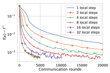
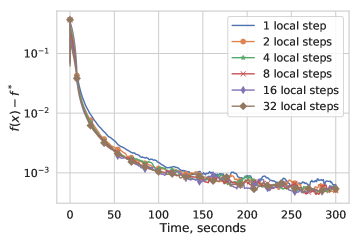
Figure 5: Results on regularized logistic regression with shared data, ‘a9a’ dataset, with stepsize $\frac{0.05}{L}$. With more local iterations, fewer communication rounds are required to get to a neighborhood of the solution.

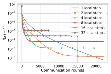
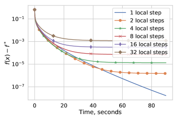
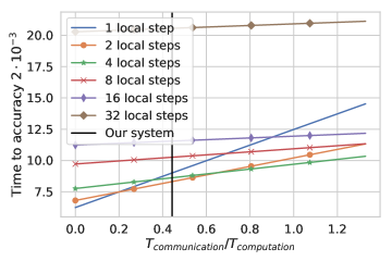
Figure 6: Same experiment as in Figure 3, performed on the ‘mushrooms’ dataset.

12 Discussion of Dieuleveut and Patel (2019)

An analysis of Local SGD for identical data under strong convexity, Lipschitzness of $\nabla f$, uniformly bounded variance, and Lipschitzness of $\nabla^{2}f$ is given in [Dieuleveut and Patel, 2019], where they obtain a similar communication complexity to [Stich, 2019] without bounded gradients. However, in the proof of their result for general non-quadratic functions (Proposition S20) they make the following assumption, rewritten in our notation:

$$G=\sup_{p}\left(1+ML_{H}\gamma\sum_{k=t_{p}}^{t_{p+1}-1}{\left\lVert\hat{x}_{k}-x_{\ast}\right\rVert}^{2}\right)<\infty,$$

where $L_{H}$ is the Lipschitz constant of the Hessian of $f$ (assumed thrice differentiable). Their discussion of $G$ speculates on the behaviour of iterate distances, e.g. saying that if they are bounded, then the guarantee is good. Unfortunately, assuming this quantity bounded implies that gradients are bounded as well, making the improvement over [Stich, 2019] unclear to us. Furthermore, as $G$ depends on the algorithm’s convergence (it is the distance from the optimum evaluated at various points), assuming it is bounded to prove convergence to a compact set results in a possibly circular argument. Since $G$ is also used as an upper bound on $H$ in their analysis, it is not possible to calculate the communication complexity.

References

- Basu et al. [2019] Debraj Basu, Deepesh Data, Can Karakus, and Suhas Diggavi. Qsparse-local-SGD: Distributed SGD with Quantization, Sparsification and Local Computations. In Advances in Neural Information Processing Systems 32, pages 14668–14679. 2019.
- Chang and Lin [2011] Chih-Chung Chang and Chih-Jen Lin. LIBSVM: A library for support vector machines. ACM Transactions on Intelligent Systems and Technology (TIST), 2(3):27, 2011.
- Chavdarova et al. [2019] Tatjana Chavdarova, Gauthier Gidel, François Fleuret, and Simon Lacoste-Julien. Reducing Noise in GAN Training with Variance Reduced Extragradient. In Advances in Neural Information Processing Systems 32, pages 391–401. Curran Associates, Inc., 2019.
- Coppola [2015] Gregory F. Coppola. Iterative parameter mixing for distributed large-margin training of structured predictors for natural language processing. PhD thesis, University of Edinburgh, UK, 2015.
- Dalcin et al. [2011] Lisandro D. Dalcin, Rodrigo R. Paz, Pablo A. Kler, and Alejandro Cosimo. Parallel distributed computing using Python. Advances in Water Resources, 34(9):1124–1139, 2011.
- Dieuleveut and Patel [2019] Aymeric Dieuleveut and Kumar Kshitij Patel. Communication trade-offs for Local-SGD with large step size. In Advances in Neural Information Processing Systems 32, pages 13579–13590. 2019.
- Gower et al. [2019] Robert Mansel Gower, Nicolas Loizou, Xun Qian, Alibek Sailanbayev, Egor Shulgin, and Peter Richtárik. SGD: General Analysis and Improved Rates. In Proceedings of the 36th International Conference on Machine Learning, volume 97 of Proceedings of Machine Learning Research, pages 5200–5209, 2019.