The detection of relativistic corrections in cosmological N-body simulations

Abstract

Cosmological N-body simulations are done on massively parallel computers. This necessitates the use of simple time integrators, and, additionally, of mesh-grid approximations of the potentials. Recently, Adamek:2015eda; Barrera-Hinojosa:2019mzo have developed general relativistic N-body simulations to capture relativistic effects mainly for cosmological purposes. We therefore ask whether, with the available technology, relativistic effects like perihelion advance can be detected numerically to a relevant precision. We first study the spurious perihelion shift in the Kepler problem, as a function of the integration method used, and then as a function of an additional interpolation of forces on a 2-dimensional lattice. This is done for several choices of eccentricities and semi-major axes. Using these results, we can predict which precisions and lattice constants allow for a detection of the relativistic perihelion advancein N-body simulation. We find that there are only small windows of parameters—such as eccentricity, distance from the central object and the Schwarzschild radius—for which the corrections can be detected in the numerics.

1 Introduction

We consider here so-called (cosmological) N-body simulations such as (Adamek2016; Springel2005; Teyssier:2001cp). In these numerical studies, potentials between the (many) particles are computed on a lattice (mesh-grid) because of the way such calculations are implemented on supercomputers. Additionally, some of these projects (such as Adamek:2015eda; Barrera-Hinojosa:2019mzo) add relativistic corrections to the forces and therefore to the trajectories of particles. The aim of our study is to give bounds on the detectability of these effects, given the computational restrictions of these large-scale projects. We will see that in many current simulations, the necessary precision to detect relativistic effects on the orbits of particles can simply not be achieved.

It is of course not difficult to devise codes which will compute the perihelion advance under relativistic corrections to arbitrary high precision. It is not the aim of our paper to study such algorithms, but rather, to see how well the integration algorithms work in the N-body simulations. In these simulations, because one considers essentially a gas of many particles, the user is restricted to rather standard integration methods, which just use the differential equations, but necessarily can not make use of the many invariants known for the (non-relativistic) Kepler problem, see e.g., (Preto:2009cp). Therefore, we need to first study the performance of standard integration schemes, such as Euler, Runge-Kutta, and Leap-Frog, because these are the methods which are widely used. We will see that only with very high precision one is able to detect the (usually quite small) relativistic corrections. Once this has been done, we can turn our attention to the effects of the discretizations (of space), which give then bounds on the necessary grid constants for which relativistic effects could be detected. We will determine parameter regions where the relativistic effects can be detected, and show that, most often, these regions are quite small.

By starting with the simple Kepler problem, in ${\mathbb{R}}^{2}$, we can concentrate on the different numerical effects in a systematic and clean way. Even so, the reader should realize that there are several quantities to be considered. The first is the numerical precision of the time integrator. We study it here in the context of the subroutines in ODEX (Hairer1993), and we also compare it to other methods, such as Euler, leapfrog (Verlet-Störmer) (Hairer2003) or Runge-Kutta with fixed time step.

To do this, we quantify the numerical errors on trajectories of particles revolving around a central object. This will allow us to give conditions which ascertain which orbits in a specific N-body simulation are precise enough to be able to measure the general relativistic perihelion shift.

After this, we consider the particle-mesh N-body scheme, as is widely used, see e.g., (Adamek2016; Springel2005). In it, forces (coming from fields and potentials) are discretized and represented on a lattice. Such elements (arnold2002) are then used to compute the values of the fields at the particles’ positions.

The force interpolation approximations are usually piecewise differentiable, and, depending on the implementations mentioned above, use different elements. It is clear that if the mesh size of the approximation (of the force) goes to 0, so will the error. But the relevant question here is to quantify what kind of phenomena can be captured, given the numerous hardware and modeling constraints.

Particle-mesh N-body simulations are used to study the evolution of particles under gravity. These codes can be used to study systems at different scales, from cosmological scales to the size of the solar system, as the methods and forces are appropriate for all scales. In the particle-mesh N-body scheme (Springel2005; Adamek2016), space-discretizations are performed to take care of the large number of particles. We analyze two common force interpolations which are used for N-body simulations purposes, namely the so-called linear and bilinear methods, which respectively correspond to first and second order interpolation. We will see that, under conditions to be specified, the effect of spatial discretization can be quite large and sometimes depends on the angle $\theta$ between the direction of the perihelion and the axes of the discrete lattice. This happens when the discretization produces discontinuous forces, i.e., for the first order force interpolation. In this case the maximal errors are proportional to the lattice constant $dx$. On the other hand, in the second order force interpolation, when one varies $\theta$, there is a small perihelion shift, fluctuating around 0. These fluctuations are seen to be of order $dx^{1.3}$. Due to the highly nonlinear step size of ODEX, we are not able to derive analytically this size of the fluctuations.

Our numerical tests show that, unless the discretization is extremely fine, the system will show an uncertainty of the perihelion, for the Kepler problem, for both force interpolation methods. Our calculations give limits on the detectability of relativistic effects, as a function of method, lattice spacing, as well as eccentricity and the relativistic parameter $\Upsilon\equiv r_{\rm sch}/r_{\rm per}$, the ratio of perihelion distance of the orbit $r_{\rm{per}}$ and the Schwarzschild radius of the central mass $r_{\rm sch}.$

2 Using standard time integrators

Our main interest is the detectability of general relativistic effects in N-body simulations, and in particular the study of discretization effects. But we first need to be sure that the time integration which is used in these projects does not already destroy the precision of the result more than the effect of the space discretization. This is the subject of this section.

A Hamiltonian problem can be integrated either as a motion in Euclidean space, or one can exploit the underlying symplectic structure of the problem. Of course, there are very good symplectic integrators, (Hairer2010), but we decided not to use them, for two reasons.

The first is that in the particle-mesh N-body codes, the Euclidean approach is used to solve the system including particles and the fields on the lattice coordinates and expressing the system in symplectic coordinates is difficult. Second, as noted in (Hairer2003) even the symplectic methods do not preserve the Runge-Lenz-Pauli vector (the orientation of the semi-major axis). This means that because of our focus on the relativistic perihelion advance, the symplectic integrators present no particular advantage. So we will stick with the classical high-order Runge-Kutta integrators ODEX (Hairer1993). Because it allows for “continuous output” we can use it to determine easily the advance of the perihelion with high precision.

We summarize those properties of ODEX which are relevant for our study. As we will be working with elements to interpolate forces, we need to explain how the algorithm deals with discontinuities. This is illustrated in (Hairer1993, Chapter II.9 and in particular, Fig. 9.6). In the interior of a plaquette, the algorithm chooses a high enough order to reach the required tolerance with a large time step $h$. On approaching the singularity, the algorithm lowers the order (to 4) but decreases $h$. In fact, the jump is approximated by a polynomial of degree 4, and this defines something like a new initial condition across the discontinuity. In the case of Runge-Kutta with fixed time step, the paper (Back2005) shows that there is a mean systematic error across the jump, which can be viewed as a weighted combination of evaluations of the vector field across the singularity.

3 Perihelion variation for time integrators with fixed time step

Here, we study the precision of perihelion calculations when working with exact forces. In later sections, we will then see how the grid discretization further affects this precision. Certainly, if we want to discriminate between non-relativistic and relativistic effects, already the integration with exact forces needs to be precise enough. This will force us to choose a small enough time step $h$.

We analyze the perihelion shift for several standard time integrators with fixed time step, namely Euler, Newton-Störmer-Verlet-leapfrog, 2nd order and 4th order Runge-Kutta.

We call the time step $h$ and we solve the Kepler problem in the form ¨x(t) = F(t, x)/m , with $x$, $v$, and $F$ in ${\mathbb{R}}^{2}$ and $m$ the mass of the object. For the convenience of the reader, we spell out these well-known methods.

Euler method

In this case, we solve (3) in the form v_ n+1 &= v_ n + a_ n h ,
x_ n+1 = x_ n+ v_ n+1 h , where $v_{n}$ is the velocity vector at time step $({n}$) which is defined as $v_{n}\equiv({x_{n}-x_{n-1}})/{h}$ and $a_{n}$ is the acceleration and is defined as the ratio of the force and mass $a_{n}\equiv a(t_{n},x_{n})=F(t_{n},x_{n})/m$. It is well-known that this implicit/backward Euler method is more stable than the explicit/forward Euler method. But it is somewhat more difficult to implement for non-linear differential equations.

Newton-Störmer-Verlet-leapfrog method

For this widely used method (sometimes called “kick-drift-kick” form of leap-frog) (Hairer2003)[Eq. 1.5], the updates are v_n+1/2 &= v_n + a_n h2 ,
x_n+1 = x_n + v_n +12 h ,
v_n+1 = v_n + 12 + a_n+1 h2  . This method is used more often as it is a symplectic method and stable and is shown to work very well for various stiff ODEs (Hairer2003).

Second order Runge-Kutta method

Finally, we will comment on the perihelion advance for the 2nd and 4th order Runge-Kutta methods (with fixed time step $h$). The Kepler problem using 2nd order Runge-Kutta algorithm—also known as midpoint method—reads, k^(1)_ x &= v_n  ,
k^(1)_ v = a_n  ,
k^(2)_ x = v_n + 12  ,
k^(2)_ v = a_n + 12  ,
x _n+1= x _n + k^(2)_ x h  ,
v _n+1= v_n + k^(2)_ v h  ,
where $k^{(1)}_{x}$ is the estimate of velocity (derivative of $x$) in time step $\rm n$, $k^{(1)}_{v}$ is the estimate of acceleration (derivative of $v$) in time step $\rm n$ and the same for $k^{(2)}_{x}$ and $k^{(2)}_{v}$. The acceleration at time $n+\frac{1}{2}$ is obtained by a_n + 12 ≡F (tn +12, xn+12)m = F (tn +12, xn+ k(1)xh/2 )m  . Also, to obtain the velocity at time $n+\frac{1}{2}$ we need to use $k^{(1)}_{v}$. The corresponding tableau for the second order Runge-Kutta method for each first order differential equation is 0 1/2 1/2 0 1  .

Fourth order Runge-Kutta method

The Kepler problem using forth order Runge-Kutta method is basically the same as second order Runge-Kutta, but with three points instead of one point in between to solve the position and velocity. The tableau we use for this method is (Butcher1963) 0 1/2 1/2 1/2 0 1/2 1 0 0 1 1/6 1/3 1/3 1/6  .

3.1 Results for various integration schemes

We solve the Kepler problem with the methods described above and find the perihelion variation for different time steps $h$. To determine the perihelion point of the orbit we choose several points near the minimum distance to the central object after each revolution. Then we fit a parabola (for Runge-Kutta, we take a 4th order polynomial to find the point closest to the central mass) and the minimum of the parabola is taken as the perihelion point. Fig. 1 illustrates how this is done, for the particular example of Mercury. The red point is the perihelion.

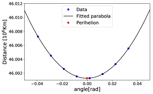
Figure 1: Detecting the spurious perihelion change for the Kepler problem for the Mercury-Sun system. For each time step of integration we determine the angle and the distance from the central body (the blue points), using the 2nd order Runge-Kutta method. We then fit a parabola through these points, and the minimum of the distance to the Sun is the red point (perihelion point). Note that the red point is very slightly to the left of 0 and shows the spurious perihelion shift due to the time integration imprecisions. We use this method to find the perihelion shift and to decrease the errors we take average over three revolutions.

The spurious shift of the perihelion of Mercury using 2nd order Runge-Kutta method with $h=0.00625$, which is the case considered in Fig. 1, is $\sim 7.8\times 10^{-5}$ radians. We measure the positions in units Giga meters ($\rm{Gm}\equiv 10^{9}$ m) , time in Mega seconds ($\rm{Ms}=10^{6}$ sec) and masses in $M_{\text{earth}}=5.972\times 10^{24}\,\rm{Kg}$. In these units, the initial position (at the perihelion), is $46.001272(\cos(\theta),\sin(\theta))$ where $\theta$ is the angle between x-axis and semi-major axis. The initial velocity is perpendicular to the line connecting Mercury and the Sun, with magnitude $58.98$. The potential is $-GM/r$ with $GM=132733$ measured in the code’s units . When we will study the problem on the lattice, the angle $\theta$ will be important. In Fig. 2 the magnitude of perihelion variation for the different time integrators and the step size $h$ is shown. The horizontal line shows the value of relativistic perihelion advance, the green/red regions respectively show where the time integrator precision is/is not good enough to observe relativistic perihelion advance. Because time integrators over- or underestimate the perihelion, we plot its absolute deviation (which for Newton’s law should be zero). This absolute value sets a limit of how small one has to take a time step $h$ to be able to detect general relativistic corrections to the orbits.

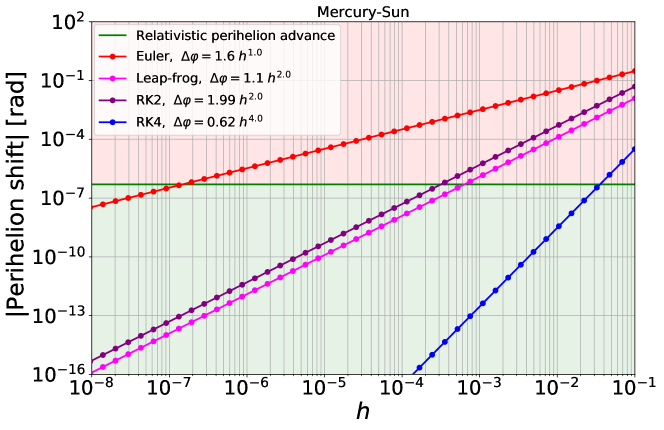
Figure 2: Achievable precision for different integrators, as a function of step size $h$. Shown is the absolute value of the perihelion shift for the Mercury-Sun problem. To make relativistic corrections distinguishable, only points in the green region are good enough. The data points correspond to $1/3$ of the advance after 3 rotations.

The relativistic parameter $\Upsilon=r_{\rm sch}/{r_{\rm per}}$ for the Mercury-Sun case with $r_{\rm per}=46\times 10^{6}$ km and $r_{\rm sch}=2.95$ km is $\Upsilon\approx 6.4\times 10^{-8}$. The eccentricity of Mercury is $\approx 0.205630$. Both parameters are considered small as the distance of Mercury to the Sun is much larger than the Schwarzschild radius of the Sun. We therefore consider also a more extreme case, where the relativistic effects are larger, such as the stars in the Galactic center known as the S-stars (Parsa) which are revolving around the central super massive black hole. For one of them, S2, the relativistic parameter at perihelion point is estimated from measurements to be $\Upsilon\approx 8.8\times 10^{-5}$, and the eccentricity is $0.884$. The details about the relativistic parameter and eccentricity can be found in Appendix LABEL:parametrization.

In our numerical study, we cover therefore a large range of these parameters. Our results are summarized for the four integration methods in Fig. 2 as a function of the time step $h$. In Fig. 3 the comparison is done as a function of $\Upsilon/\Upsilon_{0}$, where $\Upsilon_{0}$ is the relativistic parameter at perihelion point for the Mercury-Sun system. We also show the dependence on eccentricity.

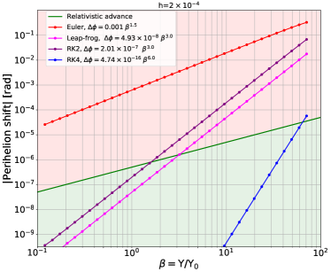
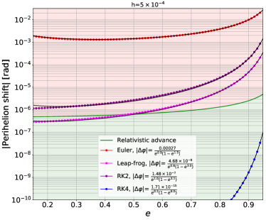
Figure 3: Left: The absolute value of the perihelion shift as a function of the normalized relativistic parameter $\beta=\Upsilon/\Upsilon_{0}$, where $\Upsilon_{0}$ is the relativistic parameter for Mercury-Sun. The red region shows where the method will fail to discriminate the relativistic perihelion advance from the integration errors (for the chosen step size of $h=0.0002$). In the green region one can safely use the method, for that specific orbit. When increasing $\beta$, the numerical perihelion shift increases, as according to (LABEL:rel_ic) the velocity of the object in the perihelion point scales like $\sqrt{\Upsilon}$, while the perihelion distance scales like $\frac{1}{\Upsilon}$. In all the methods the slope of the curve is higher than the slope of the relativistic advance curve $\Delta\varphi\sim\Upsilon$, which shows that for the orbits with large relativistic parameters, one has to choose the method and the time step very carefully. Right: The same representation as a function of eccentricity $e$. In all the methods, by increasing the eccentricity the numerical perihelion variation increases, as according to the (LABEL:ecc_ic) the velocity of the object and perihelion distance rescales respectively by $\sqrt{\frac{1+e}{1+e_{0}}}$ and ${\frac{1-e}{1-e_{0}}}$. In order to be able to measure the relativistic perihelion advance at each eccentricity we need to use the method with the appropriate step size, for example Euler and second order Runge-Kutta do not work for any eccentricity, while leapfrog is good for $e\lesssim 0.5$ and fourth order Runge-Kutta works perfectly for all eccentricities. All data points correspond to $1/3$ of the advance after 3 rotations

4 Force interpolation

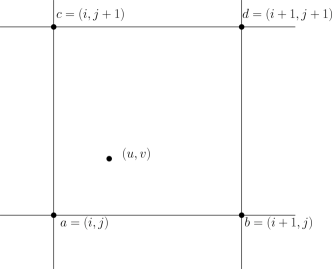
Figure 4: Notation for a plaquette on the unit mesh in ${\mathbb{R}}^{2}$.

Having considered the numerics of the classical methods, we now study the effect of discretizing space. We again restrict attention to two dimensions and set, throughout, the lattice spacing equal to $dx$. In particular, we study the two force interpolations (linear and bilinear) which are mainly used in N-body simulations, see e.g., (Springel2005) and (Adamek2016), and for which we will present numerical results. A very useful systematic derivation of finite elements for derivatives and differential complexes can be found in (arnold2002). The setup is as follows: We are given a potential $\Phi$, in our case the Newtonian potential $\Phi(x_{1},x_{2})=-GM/\sqrt{x_{1}^{2}+x_{2}^{2}}=-GM/r$, from which we want to derive the forces on the particles. In the bilinear (quadratic) method the mesh is given by integer coordinates (in ${\mathbb{Z}}^{2}$), and we assume that $\Phi$ is known in all points $(i,j)$, with $i,j\in{\mathbb{Z}}$. The force at lattice point $i,j$ is then approximated by a vector with components f^(x)_i,j &= Φi+1,j-Φi-1,j2 ,
f^(y)_i,j = Φi,j+1-Φi,j-12 .
Note that the difference is taken over 2 mesh points around the point of interest. Assume that the point $x=(u,v)\in{\mathbb{R}}^{2}$ lies in the square with corners a=(i,j) , b=(i+1,j) , c=(i,j+1) , d=(i+1,j+1) , cf. Fig. 4. We let $f_{a}^{(x)}=f_{i,j}^{(x)}$, and similarly for the other corners and the direction $(y)$.

Let $i$ be the integer part of $u$ and let $j$ be the integer part of $v$, and set $\xi=u-i$, $\eta=v-j$. The interpolated forces are then given by [eq:springel] F^(x)(u,v)=&(f^(x)_a (1-ξ)+f_b^(x)ξ)⋅(1-η) +(f^(x)_c (1-ξ)+f_d^(x)ξ)⋅η ,
F^(y)(u,v)=(f^(y)_a (1-η)+f_c^(y)η)⋅(1-ξ) +(f^(y)_b (1-η)+f_d^(y)η)⋅ξ .
Note that “$c$” and “$b$” change position between the $x$ and $y$ components.This interpolation method is called bilinear method as it is combination of two linear interpolations along the square, so it is a quadratic interpolation (arnold2002). This interpolation is continuous across the boundaries in both directions and for both components of the vector field. To verify this, one can for example restrict to the line connecting $a$ and $b$. Then $\eta=0$, and therefore one gets F^(x)(u,v)=&f^(x)_a (1-ξ)+f_b^(x)ξ ,
F^(y)(u,v)=f^(y)_a (1-ξ)+f^(y)_b ξ .
The important thing is that the values only depend on $a$ and $b$, but not on $c$ and $d$ and so continuity is guaranteed. The 3 other edges are similar.

In this scheme, as is well known, one needs 8 evaluations of $\Phi$ per plaquette. When the mesh size is $dx$ instead of $1$, all the calculations scale accordingly.

The other method, linear method which is also widely used in cosmological N-body simulations e.g., (Adamek2016) is given, with similar notation—using $g$ and $G$ instead of $f$ and $F$—by g^(x)_i,j&=Φ_i+1,j-Φ_i,j ,
g^(y)_i,j=Φ_i,j+1-Φ_i,j ,
G^(x)(u,v)=g^(x)_a(1-η)+g^(x)_cη ,
G^(y)(u,v)=g^(y)_b(1-ξ)+g^(y)_d ξ , with $a,\dots,d$ as before. This method is of lower order than the previous one, and needs fewer evaluations. The advantage is that they need less memory, but of course, it is only $1^{\rm st}$ order.

Note that if $(u,v)$ crosses the line connecting $a$ and $b$, then $G^{(x)}$ is continuous, but $G^{(y)}$ has a jump discontinuity (of order about ${\mathcal{O}}(\Phi_{i,j}-\Phi_{i+1,j})$ when $i$ and $j$ are not too close to 0). Similar considerations hold on the other boundaries of the unit plaquette.

This scheme only needs 4 evaluations of $\Phi$ per 2-dimensional plaquette, but the interpolation is not continuous. The Kepler problem can still be integrated numerically, but there will appear a spurious phase shift which is caused by the discontinuity. But the numerical errors again scale with the mesh size, albeit on a larger scale than in the first method.

We will now present the numerical results for these cases, and then discuss the limitations they imply on trajectories in N-body simulations. Of course, often calculations are done in ${\mathbb{R}}^{3}$, resp. ${\mathbb{Z}}^{3}$, but for the study of numerical issues, 2 dimensions are enough. Restriction to 1 dimension is too easy, since the two methods coincide in that case.

5 Discretization vs relativistic perihelion advance

We have seen that high precision is needed to discriminate relativistic effects in the planar two-body problem. As several N-body codes use—in addition to the standard numerical integration schemes, a discretization of space—we now study the effects of these discretizations. To concentrate on them, we use a numerical integration of very high precision (ODEX, tolerance $8\cdot 10^{-11})$ so that the effects described earlier are minimal, and the effect of discretization becomes visible.

As we want to measure the perihelion advance due to the discretization we stick to the general equations in which we do not use the symmetries of the Kepler problem. We just assume that the motion is on a plane and we solve the equations for the relative distance between two masses assuming that $m\ll M$, (˙x, ˙y) &= (v_x, v_y) ,
(˙v_x, ˙v_y)= ( H