Controlling polarization of attosecond pulses with plasmonic-enhanced bichromatic counter-rotating circularly polarised fields

Abstract

The use of bichromatic counter-rotating laser field is known to generate high-order harmonics with non-zero ellipticity. By combining such laser field with a plasmonic-enhanced spatially inhomogeneous field, we propose a way to influence the sub-cycle dynamics of the high-harmonic generation process. Using the numerical solution of the time-dependent Schrödinger equation combined with classical trajectory Monte Carlo simulations, we show that the change of the direction and the strength of the plasmonic field selectively enhances or suppresses certain recombining electron trajectories. This in turn modifies the ellipticity of the emitted attosecond pulses.

I Introduction

Control over the polarisation of attosecond pulses in extreme ultraviolet (XUV) and soft x-ray radiation is paramount to probing chiral-sensitive light-matter interactions such as x-ray magnetic circular dichroism Kfir et al. (2015); Fan et al. (2015), discrete molecular symmetries Reich and Madsen (2016); Baykusheva et al. (2016); Neufeld et al. (2019), magnetisation and spin dynamics Graves et al. (2013); Eisebitt et al. (2004); Radu et al. (2011); Boeglin et al. (2010), and recognising chirality in molecules via photoelectron circular dichroism Cireasa et al. (2015); Travnikova et al. (2010); Ferré et al. (2015) at their intrinsic timescales. Following the proposal of Becker and co-workers Eichmann et al. (1995); Milošević and Becker (2000); Milošević et al. (2000), a series of experiments have been carried out to generate high harmonics with controlled polarisation Fan et al. (2015); Kfir et al. (2015); Chen et al. (2016); Lambert et al. (2015); Fleischer et al. (2014); Ferré et al. (2015); Jiménez-Galán et al. (2017); Dorney et al. (2017). A combination of two counter-rotating circularly polarised laser pulses having fundamental ($\omega$) and its second harmonic ($2\omega$) frequency is employed to generate circularly (or elliptically) polarised high-harmonics. The resultant electric field of $\omega$-$2\omega$ combination exhibits trefoil symmetry and yields three radiation bursts per cycle of the fundamental field Eichmann et al. (1995); Milošević and Becker (2000); Milošević et al. (2000); Medišauskas et al. (2015); Jiménez-Galán et al. (2017). The resulting high-harmonic spectrum contains doublets of circularly polarised harmonics with alternating helicity. The $3n+1$ and $3n+2$ harmonics follow the polarisation of $\omega$- and $2\omega$-fields, respectively, whereas $3n$ harmonics are parity forbidden Fleischer et al. (2014); Alon et al. (1998); Milošević (2015a); Neufeld et al. (2019).

However, in High-Harmonic Generation (HHG) the control over the polarisation of the harmonics does not immediately entail the same control over the polarisation of underlying attosecond pulses. Therefore, proposals have been put forward in recent years to achieve the subcycle emission control by either modifying the underlying medium, (e.g., by choosing a suitable initial state of atoms Medišauskas et al. (2015); Milošević (2015b); Ayuso et al. (2017); Jiménez-Galán et al. (2018), using different molecular systems Yuan and Bandrauk (2013); Mauger et al. (2014)), or by modifying the laser driving schemes, (e.g., by using non-collinear bichromatic counter-rotating circularly polarised laser pulses Hernández-García et al. (2016); Hickstein et al. (2015); Huang et al. (2018), introduction of seed XUV pulse with suitable polarisation Dixit et al. (2018), tuning the ratio of the ellipticity and/or of the intensity of the bichromatic counter-rotating driving fields Jiménez-Galán et al. (2017); Dorney et al. (2017); Neufeld and Cohen (2018)), or by changing the time-delay between two driving pulses Jiménez-Galán et al. (2017); Frolov et al. (2018).

Since the experiment of Kim et al. Kim et al. (2008), a number of works have investigated the plasmonic-field assisted HHG using structured nano-objects Park et al. (2011); Pfullmann et al. (2014); Han et al. (2016); Stebbings et al. (2011); Sivis et al. (2013); Pfullmann et al. (2013); Krüger et al. (2018, 2012); Ciappina et al. (2017). Moreover, different kinds of nanostructures such as metal nanotips Krüger et al. (2018, 2012), metallic waveguides Park et al. (2011), nanoparticles Yang et al. (2013) and plasmonic antennas Sivis et al. (2013), have been explored, while many more works tried to explain HHG mediated by a plasmonic-enhanced field using numerical and theoretical methods Husakou et al. (2011a); Ciappina et al. (2012a, b); Shaaran et al. (2012); Yavuz et al. (2012); Yavuz (2013); Shaaran et al. (2013a, b); Pérez-Hernández et al. (2013); Fetić et al. (2013); He et al. (2013); Ebadi (2014); Ciappina et al. (2014); Luo et al. (2014); Chacón et al. (2015); Feng and Liu (2015); Ansari et al. (2018). Despite the abundance of research, most of the works on plasmonic-field assisted-HHG are investigating linearly polarised driving fields. In this regard, its not apparent how the high-harmonic spectrum will behave when the linearly polarised pulse in the presence of plasmonic field is replaced by BiCRCP fields. Will the pattern of circularly polarised doublets with alternating helicity be preserved throughout the spectrum? Will the increase in the energy cutoff be modified?

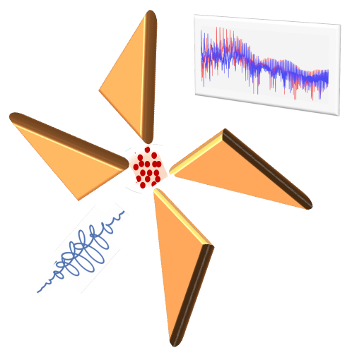
Figure 1: Conceptual illustration of the HHG driven by plasmonic-enhanced bichromatic counter-rotating circularly polarised fields. An incoming low intensity bicircular counter-rotating circularly polarised field (in blue), interacts with bowtie-shaped nano-objects and, as a result, a much higher intensity spatially nonhomogeneous laser field is generated, able to produce polarisation-resolved higher-order harmonics by the atoms located in the vicinity of the bow-tie elements.

In this work, we demonstrate, at the single atom level, the control over sub-cycle electron dynamics during HHG by combining bichromatic counter-rotating circularly polarised driving fields (BiCRCP ) with plasmonic field enhancement in a 2D geometry (see Fig. 1). The direction and strength of the plasmonic-enhanced field will provide the desired control over the sub-cycle electron dynamics, which in turn will allow us to exert influence over the attosecond pulses polarization. Atomic units are used throughout in the present work.

II Theory

In order to study HHG driven by plasmonic-enhanced BiCRCP , the time-dependent Schrödinger equation (TDSE) is solved in two spatial dimensions (2D). In the present work we give a short summary and refer the reader, for more details, to Ref. Medišauskas et al. (2015). The 2D TDSE within length gauge can be written as

$$i\frac{\partial\Psi(\mathbf{r},t)}{\partial t}=[\hat{T}+V(\mathbf{r})+\mathbf{r}\cdot\mathbf{E}^{\mathrm{total}}(\mathbf{r},t)]\Psi(\mathbf{r},t)$$ (1)

where $\hat{T}$ is the kinetic energy operator in cartesian coordinates $(x,y)$ and $\mathbf{E}^{\mathrm{total}}(\mathbf{r},t)=\mathbf{E}^{\mathrm{hf}}(t)+\mathbf{E}^{\mathrm{pl}}(\mathbf{r},t)$ is the total laser electric field, composed of the incoming laser electric spatially homogeneous field $\mathbf{E}^{\mathrm{hf}}(t)$ and the plasmon-enhanced spatial nonhomogeneous part $\mathbf{E}^{\mathrm{pl}}(\mathbf{r},t)$. Equation (1) is solved numerically for the soft-core potential given by

$$V(\mathbf{r})=-\frac{1+9\,e^{-r^{2}}}{\sqrt{r^{2}+a}},$$ (2)

where the parameter $a=2.88172$ is used to describe a 2D model neon atom. The ionisation potential of the initial $p$-orbital then results to $I_{p}$ = 0.793 a.u. ($21.6$ eV) Barth and Lein (2014). A Taylor-series propagator with expansion up to eighth order is employed to time-propagate the 2D-TDSE on a cartesian grid Moler and Van Loan (2003). We use a complex absorbing potential to avoid unphysical reflections from the boundary as

$$V_{\textrm{abs}}(\mathbf{r})=\eta(\mathbf{r}-\mathbf{r}_{0})^{n},$$ (3)

with $n=3$, $\eta=5\times 10^{-4}$ and $\mathbf{r}_{0}$ is set to $\pm 70$ a.u. in both the $x$ and $y$ directions. Finally, the temporal and spatial grid-step sizes are $dt$ = 0.005 a.u. and $dr$ = 0.2 a.u., respectively.

The incoming infra-red (IR) spatial homogeneous laser electric field has the following form:

$$\mathbf{E}^{\mathrm{hf}}(t)=E_{0}^{i}~{}g(t)~{}[E_{x}(t)~{}\hat{x}+E_{y}(t)~{}\hat{y}],$$ (4)

where $E_{0}^{i}$ is the laser electric field strength and $g(t)$ is a trapezoidal envelope with five-cycle plateau and two-cycle rising and falling edges (in units of the fundamental laser frequency $\omega$). The incoming bichromatic driving field consists of the counter-rotating fundamental field (left-handed circularly polarised) and the co-rotating second harmonic field (right-handed circularly polarised). The components $E_{x}(t)=\cos(wt)+\cos(2wt)$ and $E_{y}(t)=\sin(wt)-\sin(2wt)$ are the $x$- and $y$-components of the total driving IR field, respectively, where $\omega=0.05$ a.u., corresponding to a laser wavelength $\lambda\approx 900$ nm.

At nanometric scale, the plasmon-enhanced electric field becomes space-dependent, which significantly alters the electron dynamics. The 2D plasmonic-enhanced spatial nonhomogeneous field is, then, described as

$$\mathbf{E}^{\mathrm{pl}}(x,y,t)=E_{0}~{}g(t)~{}\left[\beta_{x}~{}h(x)~{}E_{x}(t)~{}\hat{x}+\beta_{y}~{}h(y)~{}E_{y}(t)~{}\hat{y}\right].$$ (5)

In our study we set $E_{0}=0.05$ a.u., that corresponds to a laser intensity $I=E_{0}^{2}\approx 9\times 10^{13}$ W/cm², large enough as to generate HHG out of a set of atoms. Note that, typically, there exists an enhancement factor of several orders of magnitude between $E_{0}$ and $E_{0}^{i}$, i.e. $E_{0}=\alpha E_{0}^{i}$. In our case, and considering an incoming laser intensity of about 10¹¹ W/cm², $\alpha\approx 100$. The parameters $\beta_{x}$ and $\beta_{y}$ characterises the strengths of the plasmonic field along the $x$- and $y$-directions, respectively. The spatial inhomogeneity $h$ is typically approximated to linear order, i.e., $h(x)=x$ and $h(y)=y$ Husakou et al. (2011b); Ciappina et al. (2012a); Yavuz et al. (2012); Ansari et al. (2018), which is the chosen form in our model too, and gives the dimension of inverse length to $\beta_{x/y}$. As it is discussed in Ref. Ciappina et al. (2012a), the inverse of $\beta$ defines the spatial inhomogeneity region, i.e. the spatial region where the field present noticeable spatial variations. For instance, a $\beta=0.01$ a.u corresponds to an inhomogeneity region of 100 a.u. (5.3 nm) (see next Section). This number appears to be compatible with, for instance, a distance between the bow-ties element apexes of around 10 nm. The values of $\beta_{x}$ and $\beta_{y}$ can be tuned independently, for instance, changing the distance between the bowties apexes in either the $x$ or $y$ direction. Typically, if one chose the plasmonic nanostructure to be resonant with the incoming driving frequency, the plasmonic-enhanced field is an ’amplified’ copy of the incoming one, with a maximum enhancement factor. As the plasmonic field development is not instantaneous, some phase difference between the incoming and outgoing fields can be observed Schötz et al. (2017). For long pulses, as the ones used in this work, this phase difference is irrelevant. For the case of bichromatic driving fields, where two frequencies come into play, it would be more difficult to find the resonance condition, engineering the plasmonic nanostructures. As we are not interested in maximizing the amplification factor, this is not an issue. In principle, different time delays will appear for each of the two colors, but nowadays there exists enough time resolution as to control the incoming field in a way to compensate any phase difference inherited in the plasmonic-enhanced field.

From an experimental viewpoint, the seminal experiment of Kim et al. Kim et al. (2008) was put under controversy several years after Sivis et al. (2012). In short, one of the problematic points was indeed the conversion efficiency of the nanostructure-enhanced HHG. Meanwhile Sivis et al Sivis et al. (2012), argued that the ratio between nanostructure-enhanced and conventional HHG is $\lesssim 10^{-8}$, Kim et al. Kim et al. (2012), concluded that the ratio reached $10^{-6}$. The latter is obtained using a total number of atoms equal to $\approx 8\times 10^{4}$ atoms, in a total interaction volume of 60 nm x 50 nm x 50 nm x 150 bow-ties at 115 torr pressure (for more details see Ref. Kim et al. (2012)). Another point to take into account is that the signal could contain atomic lines emission, that could prevent to observe a ‘clean’ HHG signal Sivis et al. (2013). We are aware that the extraction of a measurable and ‘bright’ HHG signal from the original Kim’s setup could be demanding, but, as it is discussed in Sivis et al. (2012); Kim et al. (2012) and presented in Park et al. (2011), there exist another setups, where it would be possible to extract a more realistic number of HHG photons. From a theoretical viewpoint, however, we only would need to deal with a spatial inhomogeneous field, generated with whatever nanostructure setup, and using any target as a driven media. For instance, it is nowadays well established that the interband HHG in solid materials resembles to a great extent the atomic/molecular HHG. Therefore, if we consider a setup as the one presented in Ref. Han et al. (2016), it would be possible to apply our proposal to a piece of solid, embedded in a plasmonic nanostructure. Here, several problems are solved, namely (i) there is no risk to observe atomic lines emission and (ii) even when the interaction volume is comparable to the previous (atomic) case, the density of the solid would make the HHG signal larger.

A final remark about our single atom model. It is true that any displacement of the atom in the interaction region will change the modulations and the structure of the HHG emission. There is, however, one point to consider. A measurable HHG signal will be only possible if the plasmonic-enhanced field exceed the value needed for the HHG process to happen. In this way, not all the atoms will ‘feel’ an electric field able to generate HHG. This last aspect could enter in contradiction with some of the previous points, i.e. we are reducing the interaction volume (number of atoms) even more, what would make the measurement of an HHG signal even more arduous. On the other hand, it is not the intention of the present work to cover both the microscopic and macroscopic/collective aspects (coherence of the emitted radiation, phase matching, etc.) of the process, but to present a ‘proof of principle’, in the sense to show and study, at a single atom level, how a plasmonic-enhanced 2D field is able to control the polarization of the generated attosecond pulses.

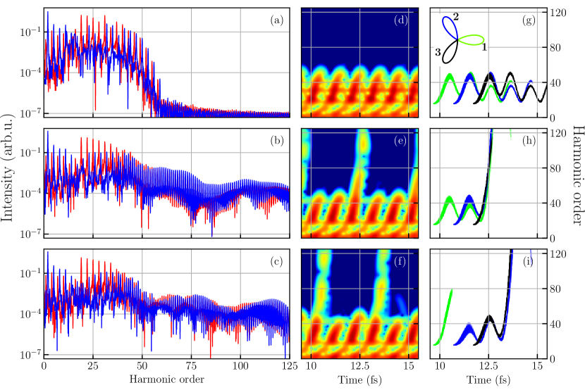
Figure 2: High-order harmonic spectra (a-c) and time-frequency maps (d-f) calculated by solving 2D-TDSE. (g-i) represent the return-energy versus -time of the ionized electrons calculated from classical trajectory Monte-Carlo simulations. The harmonics plotted in red (or blue) colour in Fig. (a-c) are right- (or left-) circularly polarized. The Lissajous figure of the total bichromatic counter-rotating circularly polarised driving field is trefoil and shown in the inset. The field lobes are marked numerically as they are traversed in time, i.e., in time, the field follows the order 1-2-3 of the lobes. Also, the field lobes are colour-coded with respect to their ionization and recombination times. In other words, the return-energy and -time of the electron which was ionized during, say, lobe 1 (green) is represented by green color in Figs. (g-i). Moreover, the first row [Figs. (a), (d), and (g)] is obtained for the spatially homogeneous field, i.e., $\beta_{x}=\beta_{y}=0$. The second [Figs. (b), (e), and (h)] and third [Figs. (c), (f), and (i)] rows correspond to the cases when the plasmonic field is applied along x-axis ($\beta_{x}=0.01$ a.u.; $\beta_{y}=0$) and along y-axis ($\beta_{x}=0;$ $\beta_{y}=0.01$ a.u.), respectively (see the text for more details).

III Results

Figure 2(a) shows the reference harmonic spectrum obtained for the spatial homogeneous case with $\mathbf{E}^{\mathrm{pl}}=0$. To obtain the resultant harmonic spectrum, the electron is assumed to be emitted from the two degenerate atomic $p$-states, i.e., $p+$ ($l=1,m=+1$) and $p-$ ($l=1,m=-1$) and then, both the contributions are added coherently. Also, the time-dependent dipole was converted to a right/left circularly polarised basis by using $d_{\pm}=[d_{x}(t)\pm id_{y}(t)]/\sqrt{2}$, where $d_{x/y}(t)$ are the net time-dependent dipoles along $x/y-$coordinates. The obtained reference spectrum consists of $3n+1$ and $3n+2$ harmonics exhibiting right (red) and left-handed (blue) circular polarisations, respectively, and the $3n$ harmonics are absent. This was studied in detail in previous works Medišauskas et al. (2015); Jiménez-Galán et al. (2017); Milošević (2015a); Neufeld et al. (2019); Jiménez-Galán et al. (2018). The reference spectrum also shows a clear energy cutoff at around $\approx 50^{\textrm{th}}$ harmonic order, which is consistent with the cutoff law for BiCRCP fields of equal intensity Milošević et al. (2000). Elliptically polarised attosecond pulses are expected since the spectral intensities of harmonics with opposite helicity are different Medišauskas et al. (2015).

Figures 2(b) and (c) present plasmonic field assisted harmonic spectra with $\beta_{x}=0.01$ a.u. ($\beta_{y}=0$) and $\beta_{y}=0.01$ a.u. ($\beta_{x}=0$), respectively. The spectra are drastically different in comparison to the reference case of Fig. 2(a). First, there is a significant increase in the energy cutoff, which is a general feature of plasmonic-enhanced HHG Ciappina et al. (2012a, b); Shaaran et al. (2012); Yavuz et al. (2012); Yavuz (2013); Shaaran et al. (2013a, b); Pérez-Hernández et al. (2013); Fetić et al. (2013); He et al. (2013); Ebadi (2014); Ciappina et al. (2014); Luo et al. (2014); Chacón et al. (2015); Feng and Liu (2015); Ansari et al. (2018). Second, harmonics of order $3n$ appear in the spectra for higher orders, which is also expected, since the spatially-dependent plasmonic field $\mathbf{E}^{\mathrm{pl}}$ breaks the trefoil symmetry of the incoming field $\mathbf{E}^{\mathrm{total}}$. Furthermore, above $~{}35^{\textrm{th}}$ order the right- and left-circularly polarized harmonics overlap with approximately equal intensities and have no apparent selection rules. This is a strong indication that the harmonics above the $35^{\textrm{th}}$ order originate from linearly or low-elliptically polarised attosecond pulses generated once per laser cycle. Note, that the differences in the spectra are sensitive to the direction of the plasmonic field since the spectra in Figs. 2(b) and (c) are different.

To connect the changes of the harmonic spectra with the underlying sub-cycle electron dynamics, we obtain time-frequency maps by performing a Gabor transform of the time-dependent total dipole

$$\tilde{d}_{x,y}(\Omega,t_{0})=\frac{1}{2\pi}\int\mathrm{d}t\ d_{x,y}(t)~{}e^{-i\Omega t}e^{-\frac{(t-t_{0})^{2}}{(2\sigma^{2})}}$$ (6)

with $\sigma=1/(3\omega)$. In the time-frequency map of the reference spectrum, the pair of short and long trajectories can be seen, which resemble the rising and falling edges of a gaussian curve, respectively. It is evident that the short trajectories are dominant. The reason can be found by analysing the harmonic generation process via semiclassical three-step model. The model gives a complex travel time of the electron in continuum owing to its generation by tunnelling. The imaginary part of the travel time gives the probability of the process whereas the real part decides the energy of the harmonic. Milošević and co-workers Milošević et al. (2000) have showed that the imaginary part peaks at approximately $T/3$ and drops substantially after half-a-cycle of the fundamental field and thus, explained the major contribution of the harmonics produced by the short trajectory electrons. Also, it can be seen that three bursts of radiation of equal strengths (originated from short trajectories) are produced during each cycle $T\approx 2.6$ fs of the fundamental field (see Fig. 2(d)). It can be understood by the Lissajous figure of the total field, which shows that the total electric field reaches its maximum three times during a single cycle of the fundamental field (trefoil symmetry; see inset in Fig. 2(g)).

To further interpret the continuum electron dynamics and underlying HHG process, we use classical trajectory Monte Carlo (CTMC) simulations. Details of the CTMC calculation can be found in Hofmann et al. (2018) and references therein. In addition to an ADK initial transverse momentum distribution Ammosov et al. (1986); Delone and Krainov (1991), a Gaussian distribution of initial longitudinal momentum was allowed Hofmann et al. (2013, 2014).

The return-times and -energies of the ionized electrons in the reference driving field obtained from the CTMC calculations are shown in Fig. 2(g). The return condition for each trajectory was a shorter distance to the ion than the individual exit radius, which is known to reproduce TDSE and experimental results Xiong et al. (2015); Hofmann et al. (2018). The CTMC trajectories are grouped according to the ionisation events occurring during one of the three lobes of the driving field, indicated by different colors in Fig. 2(g). Comparing Figs. 2(d) and (g) we see that the CTMC calculations reproduce the Gabor analysis well. Furthermore, it is made clear that the main features in the reference spectra are produced by the short electron trajectories, i.e., the electrons that return during the next lobe of the field after their ionization. This is in good agreement with trajectory-based studies of HHG in bi-chromatic counter-rotating field Zhang et al. (2016).

As we have seen in Figs. 2(a-b), the plasmonic field tends to break the symmetry of the harmonic spectra. In contrast, the time-frequency maps in Figs. 2(d-e) reveal a very regular sub-cycle dynamics. The effect of the (symmetry-breaking) plasmonic field is to enhance (or suppress) the energy-cutoff of attosecond bursts of radiation produced during each lobe of the driving laser field. When the plasmonic field is along the $x$-direction (parallel to one of the field maxima directions) in Figs. 2(b),(e) and (h), those short trajectories which are ionised during a lobe immediately before the laser field aligns with the plasmonic field have enhanced kinetic energy (say, the trajectory shown in black color in Fig. 2(h)). Although the long trajectories does show an enhancement in harmonic energy, they have minimal probability leading to their negligible contribution in harmonic spectra. The picture changes completely when the plasmonic field is oriented along $y$-direction (30^∘ from the nearest field maximum) in Figs. 2(c),(f) and (i). Here, the short trajectories ionised during the second lobe of the field return with reduced energy, while short trajectories ionised during the first lobe and long trajectories from both others contribute to the enhanced harmonics.

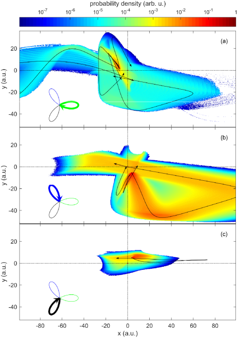
Figure 3: Classical electron trajectories, which are returning back to the parent ion, ionised during three different lobes of the field. The plasmonic field is employed along $x$-direction with $\beta_{x}$ = 0.01 a.u. Some exemplary trajectories are highlighted by black arrows. The insets indicate the lobe during which the ionization takes place and the rotation direction of the laser electric field vector.

The enhancement of attosecond radiation bursts becomes clear, when looking at the probability density maps of returning trajectories in Fig. 3. They are obtained by CTMC simulation, for ionisation during each lobe of the total field and for the plasmonic field applied along $x$-direction ($\beta_{x}$ = 0.01 a.u.). If the electron is ionized during the lobes 1 or 2, the excursion of its returning trajectory can be much further and these electrons can recombine during the next several lobes after ionization [see Figs. 3(a) and (b)]. Contrarily, only short trajectories return when an electron is ionised during lobe 3 and recombines during lobe 1 of the next cycle [see Fig. 3(c)].

Trajectories returning towards the ion from the positive $x$-axis are those which yield harmonics with enhanced cut-off energy [compare Fig. 3 and Fig. 2(h)]. In this case, both the direction of the applied plasmonic field and the direction of the driving field coincides with the direction of returning photoelectron such that the electron feels the maximum acceleration upon return and accumulates more kinetic energy. Similar reasoning can be used if we apply the plasmonic field along $y$-direction ($\beta_{y}$ = 0.01 a.u.). In this case, higher energy photons are produced when photoelectrons recombine during lobe 2 of the field, see again Fig. 2(i). If we reverse the helicity of the laser field, i.e., choosing negative helicity for the $\omega-$field and positive helicity for the $2\omega-$field, the order of the lobes followed by the net bicircular field will change. It means that instead of lobes 1-2-3, the order becomes 1-3-2 in time. By considering the reverse helicity field, while keeping $\beta_{y}=0.01$ a.u., the short trajectories returning at approximately $12$ fs will be enhanced because they are ionised when the field points mostly along negative $y$-direction and return from positive $y$-direction during the next lobe (not shown here). This is different than the case shown in Figs. 2(b), (e) and (h) when $\beta_{x}=0.01$ lead to the enhancement of trajectory returning at $12$ fs.

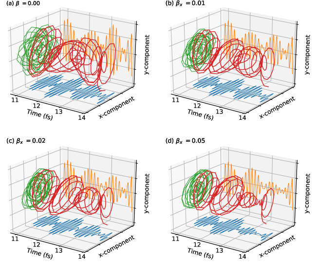
Figure 4: The total time-dependent electric field (in red) corresponding to an attosecond pulse train for different strength of plasmonic field along $x$-direction. The x-component (in blue), y-component (in orange) and Lissajous figure (in green) of the total field are also shown. $18-24^{\textrm{th}}$ harmonics window is used to synthesis an attosecond pulse train.

So far we have discussed only the results for a plasmonic field with strength $\beta_{x,y}=0.01$ a.u., for which the polarisation and position of the harmonics below the cut-off energy remain largely unaffected. As the strength of the plasmonic field is increased to $\beta_{x,y}$ = 0.02 and 0.05 a.u., the below-cutoff harmonic spectrum undergoes a substantial change with the appearance of $3n$ harmonics, and right- and left-handed harmonics overlapping with equal strength. This modification is driven by the change of polarisation of the underlying attosecond pulses. We demonstrate this change by plotting, in Fig. 4, the total electric field and its $x$- and $y$-components for a window between the $18^{\textrm{th}}-24^{\textrm{th}}$ harmonics and for different plasmonic field strengths.

For the homogeneous case in Fig. 4(a), the attosecond pulses have elliptical polarization, where the major polarization axis is rotated by 120^∘ for each pulse. This is a direct consequence of unequal intensities of the $3n+1$ and $3n+2$ harmonics and the trefoil symmetry of the BiCRCP field Medišauskas et al. (2015); Jiménez-Galán et al. (2017); Dorney et al. (2017); Neufeld and Cohen (2018); Milošević (2015a). Indeed, if we look at the electric field generated by the harmonics around the harmonic cut-off energy, where both $3n+1$ and $3n+2$ harmonic intensities are similar [see Fig. 2(a)], the attosecond pulses would show a near-linear polarization with the polarization direction rotated by 120^∘ for each consecutive pulse.

As the strength of the plasmonic field increases, the polarization of one radiation burst (emitted at around 13 fs in Fig. 4), changes to circular and its amplitude is suppressed. Meanwhile, the major polarization axis of the other two radiation bursts aligns to a common direction. When the plasmonic field is applied along the $y$-direction (not shown here), analogous findings can be applied, with the difference that: (i) a weaker plasmonic field ($\beta_{y}=0.01$ a.u.) is already sufficient to align the polarization ellipses of the generated attosecond pulses and (ii) suppression of one of the radiation bursts occurs only for stronger field strengths.

Beyond the harmonic cut-off energy, the emitted radiation has linear polarization with a direction that coincides with that of the applied plasmonic field. Consequently, all the harmonics including $3n$-harmonics have comparable intensities. For example, the electric field obtained by filtering out $60^{\textrm{th}}-66^{\textrm{th}}$ harmonics has a linear polarization along $x$- ($y$-) direction when $\beta_{x}\neq 0.00$ ($\beta_{y}\neq 0.00$). The same is true for the electric field generated by $78^{\textrm{th}}-84^{\textrm{th}}$ harmonics.

This observation corresponds to what we have already seen from the CTMC analysis. The HHG spectrum above the reference cut-off energy stems from the photoelectrons that return to the parent ion from the direction of the plasmonic field and therefore, are additionally accelerated to higher kinetic energy. However, since the additional acceleration occurs only along the plasmonic field direction, the high-energy radiation is linearly polarized and is emitted only once per laser cycle. Any photoelectron trajectories returning and recombining from a different angle will only contribute to the lower energy part of the HHG spectrum.

IV Conclusions

In summary, while the HHG process driven by BiCRCP laser field follows the three-fold symmetry pattern, adding a local plasmonic field along a particular spatial dimension modifies the sub-cycle electron dynamics in non-trivial ways: enhancing some long or short photoelectron trajectories while suppressing some others. Simply by changing the direction of plasmonic field enhancement, rich yet predictable control of electron trajectories is possible, providing as yet unexplored possibilities for sub-cycle control of the HHG process. Furthermore, the modification of the sub-cycle electron dynamics also leads to subtle changes in the polarization of the emitted high-harmonic radiation. For instance, by filtering appropriate harmonic orders, an attosecond pulse train consisting of nearly-circularly, elliptically or linearly polarised pulses is achieved. Alternatively, by changing the plasmonic field intensity, a predefined major axis direction is enforced for all elliptically polarized pulses in an attosecond pulse train. The plasmonic field intensity can be tuned by geometrically engineering plasmonic nanostructures with different sizes and shapes.