Intelligent Reflecting Surface Aided Multigroup Multicast MISO Communication Systems

Abstract

Intelligent reflecting surface (IRS) has recently been envisioned to offer unprecedented massive multiple-input multiple-output (MIMO)-like gains by deploying large-scale and low-cost passive reflection elements. By adjusting the reflection coefficients, the IRS can change the phase shifts on the impinging electromagnetic waves so that it can smartly reconfigure the signal propagation environment and enhance the power of the desired received signal or suppress the interference signal. In this paper, we consider downlink multigroup multicast communication systems assisted by an IRS. We aim for maximizing the sum rate of all the multicasting groups by the joint optimization of the precoding matrix at the base station (BS) and the reflection coefficients at the IRS under both the power and unit-modulus constraint. To tackle this non-convex problem, we propose two efficient algorithms under the majorization–minimization (MM) algorithm framework. Specifically, a concave lower bound surrogate objective function of each user’s rate has been derived firstly, based on which two sets of variables can be updated alternately by solving two corresponding second-order cone programming (SOCP) problems. Then, in order to reduce the computational complexity, we derive another concave lower bound function of each group’s rate for each set of variables at every iteration, and obtain the closed-form solutions under these loose surrogate objective functions. Finally, the simulation results demonstrate the benefits in terms of the spectral and energy efficiency of the introduced IRS and the effectiveness in terms of the convergence and complexity of our proposed algorithms.

I Introduction

In the era of 5G and Internet of Things by 2020, it is predicted that the network capacity will increase by 1000 folds to serve at least 50 billions devices through wireless communications [1] and the capacity is expected to be achieved with lower energy consumption. To meet those Quality of Service (QoS) requirements, intelligent reflecting surface (IRS), as a promising new technology, has been proposed recently to achieve high spectral and energy efficiency. It is an artificial passive radio array structure where the phase of each passive element on the surface can be adjusted continuously or discretely with low power consumption [2, 3], and then change the directions of the reflected signal into the specific receivers to enhance the received signal power [4, 5, 6, 7] or suppress interference as well as enhance security/privacy [8, 9].

The IRS, as a new concept beyond conventional massive multiple-input and multiple-output (MIMO) systems, maintains all the advantages of massive MIMO systems, such as being capable of focusing large amounts of energy in three-dimensional space which paves the way for wireless charging, remote sensing and data transmissions. However, the differences between IRS and massive MIMO are also obvious. Firstly, the IRS can be densely deployed in indoor spaces, making it possible to provide high data rates for indoor devices in the way of near-field communications [10]. Secondly, in contrast to conventional active antenna array equipped with energy-consuming radio frequency chains and power amplifiers, the IRS with passive reflection elements is cost-effective and energy-efficient [4], which enables IRS to be a prospective energy-efficient technology in green communications. Thirdly, as the IRS just reflects the signal in a passive way, there is no thermal noise or self-interference imposed on the received signal as in conventional full-duplex relays.

Due to these significant advantages, IRS has been investigated in various wireless communication systems. Specifically, the authors in [4] first formulated the joint active and passive beamforming design problem both in downlink single-user and multiple-users multiple-input single-output (MISO) systems assisted by the IRS, while the total transmit power of the base station (BS) is minimized based on the semidefinite relaxation (SDR) [11] and alternating optimization (AO) techniques. In order to reduce the high computational complexity incurred by SDR, Yu et al. proposed low complexity algorithms based on MM (Majorization–Minimization or Minorization–Maximization) algorithm in [8] and manifold optimization in [12] to design reflection coefficients with the targets of maximizing the security capacity and spectral efficiency communications, respectively. Pan et al. considered the weighted sum rate maximization problems in multicell MIMO communications [5], simultaneous wireless information and power transfer (SWIPT) aided systems [6], artificial-noise-aided secure MIMO communications [9], all demonstrating the significant performance gains achieved by deploying an IRS in the networks. A deep reinforcement learning (DRL)-based algorithm [7] and a mobile edge computing-based algorithm [13] were proposed to jointly design the active and passive beamformings in IRS-related systems. In cognitive radio (CR) communication systems, the high rate for the secondary user (SU) can be acheived with the assistance of the IRS [14].

However, all the above-mentioned contributions only investigated the performance benefits of deploying an IRS in unicast transmissions, where the BS sends an independent data stream to each user. However, unicast transmissions will cause severe interference and high system complexity when the number of users is large. To address this issue, the multicast transmission based on content reuse [15] (e.g., identical content may be requested by a group of users simultaneously) has attracted wide attention, especially for the application scenarios such as popular TV programme or video conference. From the perspective of operators, it can be envisioned that multicast transmission is capable of effectively alleviating the pressure of tremendous wireless data traffic and play a vital role in the next generation wireless networks. Therefore, it is necessary to explore the potential performance benefits brought by an IRS during the multigroup multicast transmission. In specifically, in multicast systems, the data rate of each group is limited by the user with the worst-channel gains. Hence, the IRS can be deployed to improve the channel conditions of the worst-case user, which can be significantly improve the system performance.

A common performance metric in multicast transmissions is the max-min fairness (MMF), where the minimum signal-to-interference-plus-noise-ratio (SINR) or spectral efficiency of users in each multicasting group or among all multicasting groups is maximized [16, 17, 18, 19, 20]. Prior seminal treatments of multicast transmission in single-group and multigroup are presented in [16, 17], where the MMF problems are formulated as a fractional second-order cone programming (SOCP) and are NP-hard in general. The SDR technique [11] was adopted to approximately solve the SOCP problem with some mathematical manipulations. In order to reduce the high computational complexity of SDR, several low-complexity algorithms, such as successive convex approximation approach in the single-group multicast scenario [18], asymptotic approach [19] and heuristic algorithm [20] in the multigroup multicast scenario, have been proposed by exploiting the special feature of near-orthogonal massive MIMO channels.

In this paper, we consider an IRS-assisted multigroup multicast transmission system in which a multiple-antenna BS transmits independent information data streams to multiple groups, and the single-antenna users in the same group share the same information and suffer from interference from those signals sent to other groups. Unfortunately, the popular SDR-based method incurs a high computational complexity which hinders its practical implementation when the number of design parameters (e.g., precoding matrix and reflection coefficient vector) becomes large. Furthermore, the aforementioned low-complexity techniques designed for the IRS-aided unicast communication schemes cannot be directly applied in the multigroup multicast communication systems since the MMF metric is a non-differentiable and complex objective function.

Against the above background, the main contributions of our work are summarized as follows:

• To the best of our knowledge, this is the first work exploring the performance benefits of deploying an IRS in multigroup multicast communication systems. Specifically, we jointly optimize the precoding matrix and the reflection coefficient vector to maximize the sum rate of all the multicasting groups, where the rate of each multicasting group is limited by the minimum rate of users in the group. This formulated problem is much more challenging than previous problems considered in unicast systems since our considered objective function is non-differentiable and complex due to the nature of the multicast transmission mechanism. In addition, the highly coupled variables and complex sum rate expression aggravates the difficulty to solve this problem.

• The formulated problem is solved efficiently in an iterative manner based on the alternating optimization method under the MM algorithm framework. Specifically, we firstly minorize the original non-concave objective function by a surrogate function which is biconcave of precoding matrix and reflection coefficient vector, and then apply the alternating optimization method to decouple those variables. At each iteration of the alternating optimization method, the subproblem corresponding to each set of variables is reformulated as an SOCP problem by introducing auxiliary variables, which can help to transform the non-differentiable concave objective function into a series of convex constraints.

• To further reduce the computational complexity, we use the MM method to derive closed-form solutions of each subproblem, instead of solving the complex SOCP problems with a high complexity at each iteration. Specifically, we firstly apply the log-sum-exp lower bound to approximate the non-differentiable concave objective function, yielding a differentiable concave function. Then, we derive a tractable surrogate objective function of the log-sum-exp function, based on which we derive the closed-form solutions of each subproblem. Finally, we prove that the proposed algorithm is guaranteed to converge and the solution sequences generated by the algorithm converge to KKT points.

• Finally, the simulation results demonstrate the superiority of the IRS-assisted multigroup multicast system over conventional massive MIMO systems in terms of the spectral efficiency and energy efficiency. The convergence and the low complexity of the proposed algorithms have also been illustrated.

The remainder of this paper is organized as follows. Section II introduces the system model and formulates the optimization problem. An SOCP-based method is developed to solve the problem in Section III. Section IV further provides a low-complexity algorithm. Finally, Section V and Section VI show the simulation results and conclusions, respectively.

Notations: The following mathematical notations and symbols are used throughout this paper. Vectors and matrices are denoted by boldface lowercase letters and boldface uppercase letters, respectively. The symbols $\mathbf{X}^{*}$, $\mathbf{X}^{\mathrm{T}}$, $\mathbf{X}^{\mathrm{H}}$, and $||\mathbf{X}||_{F}$ denote the conjugate, transpose, Hermitian (conjugate transpose), Frobenius norm of matrix $\mathbf{X}$, respectively. The symbols $||\mathbf{x}||_{1}$ and $||\mathbf{x}||_{2}$ denote 1-norm and 2-norm of vector $\mathbf{x}$, respectively. The symbols $\mathrm{Tr}\{\cdot\}$, $\mathrm{Re}\{\cdot\}$, $|\cdot|$, and $\angle\left(\cdot\right)$ denote the trace, real part, modulus and angle of a complex number, respectively. $\mathrm{diag}(\mathbf{x})$ is a diagonal matrix with the entries of $\mathbf{x}$ on its main diagonal. $[\mathbf{x}]_{m}$ means the $m^{\mathrm{th}}$ element of the vector $\mathbf{x}$. The Kronecker product between two matrices $\mathbf{X}$ and $\mathbf{Y}$ is denoted by $\mathbf{X}\otimes\mathbf{Y}$. $\mathbf{X}\succeq\mathbf{Y}$means that $\mathbf{X}-\mathbf{Y}$ is positive semidefinite. Additionally, the symbol $\mathbb{C}$ denotes complex field, $\mathbb{R}$ represents real field, and $j\triangleq\sqrt{-1}$ is the imaginary unit.

II System Model

II-A Signal Transmission Model

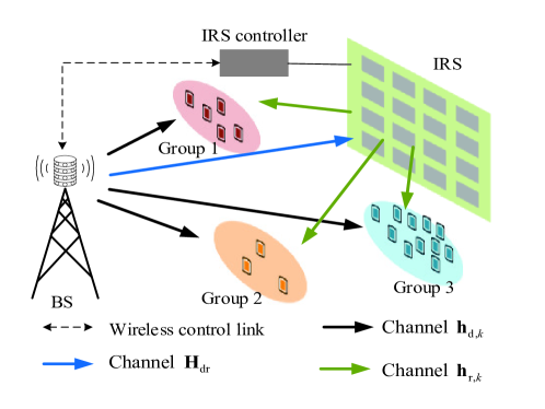
Figure 1: An IRS-aided multigroup multicast communication system.

As shown in Fig. 1, we consider an IRS-aided multigroup multicast MISO communication system. There is a BS with $N$ transmit antennas serving $G$ multicasting groups. Users in the same group share the same information data and the information data destined for different groups are independent and different, which means there exists inter-group interference. Let us define the set of all multicast groups by $\mathcal{G}=\{1,2,...,G\}$. Assuming that there are $K(K\geq G)$ users in total, the user set belonging to group $g\in\mathcal{G}$ is denoted as $\mathcal{K}_{g}$ and each user can only belong to one group, i.e., $\mathcal{K}_{i}$$\cap$$\mathcal{K}_{j}$=$\emptyset,\forall i,j\in\mathcal{G},i\neq j$. The transmit signal at the BS is

$${\bf x}=\sum\limits_{g=1}^{G}{\bf f}_{g}s_{g},$$ (1)

where $s_{g}$ is the desired independent Gaussian data symbol of group $g$ and follows $\mathbb{E}[|s_{g}|^{2}]=1$ as well as ${\bf f}_{g}\in\mathbb{C}^{N\times 1}$ is the corresponding precoding vector. Let us denote the collection of all precoding vectors as $\mathbf{F=}[{\bf\mathbf{f}}_{1},\cdots,{\bf\mathbf{f}}_{G}]\in\mathbb{C}^{N\times G}$ satisfying the power constraint $\mathcal{S}_{F}=\{\mathbf{F}\mid\mathrm{Tr}\left[\mathbf{F}^{\mathrm{H}}\mathbf{F}\right]\leq P_{\mathrm{T}}\}$, where $P_{\mathrm{T}}$ is the maximum available transmit power at the BS.

In the multigroup multicast system, we propose to employ an IRS with the goal of enhancing the received signal strength of users by reflecting signals from the BS to the users. It is assumed that the signal power of the multi-reflections (i.e., reflections more than once) on the IRS is ignored due to the severe path loss [4]. Denote $M$ as the number of the reflection elements on the IRS, then the reflection coefficient matrix of the IRS is modeled by a diagonal matrix $\mathbf{E}=\mathrm{diag}([e_{1},\cdots,e_{M}]^{\mathrm{T}})\in\mathbb{C}^{M\times M}$, where $|e_{m}|^{2}=1,\forall m=1,\cdots,M$ [4]. Please note that the design of the practical reflection amplitude which was modeled as a function of the phase shifts [21] is more complex and will be investigated in our future work. The channels spanning from the BS to user $k$, from the BS to the IRS, and from the IRS to user $k$ are denoted by $\mathbf{h}_{\mathrm{d},k}\in\mathbb{C}^{N\times 1}$, $\mathbf{H_{\mathrm{dr}}}\in\mathbb{C}^{M\times N}$, and $\mathbf{h}_{\mathrm{r},k}\in\mathbb{C}^{M\times 1}$, respectively.

It is assumed that the channel state information (CSI) is perfectly known at the BS. The BS is responsible for designing the reflection coefficients of the IRS and sends them back to the IRS controller as shown in Fig. 1. As a result, the received signal of user $k\in\mathcal{K}_{g}$ belonging to group $g$ is

$$y_{k}=(\mathbf{h}_{\mathrm{d},k}^{\mathrm{H}}+\mathbf{h}_{\mathrm{r},k}^{\mathrm{H}}\mathbf{E}\mathbf{H_{\mathrm{dr}}})\sum\limits_{g=1}^{G}{\bf f}_{g}s_{g}+n_{k},$$ (2)

where $n_{k}$ is the received noise at user $k$, which is an additive white Gaussian noise (AWGN) following circularly symmetric complex Gaussian (CSCG) distribution with zero mean and variance $\sigma_{k}^{2}$. Then, its achievable data rate (bps/Hz) is given by

$$R_{k}=\log_{2}\left(1+\frac{|(\mathbf{h}_{\mathrm{d},k}^{\mathrm{H}}+\mathbf{h}_{\mathrm{r},k}^{\mathrm{H}}\mathbf{E}\mathbf{H_{\mathrm{dr}}}){\bf f}_{g}|^{2}}{\sum_{i\neq g}^{G}|(\mathbf{h}_{\mathrm{d},k}^{\mathrm{H}}+\mathbf{h}_{\mathrm{r},k}^{\mathrm{H}}\mathbf{E}\mathbf{H_{\mathrm{dr}}}){\bf f}_{i}|^{2}+\sigma_{k}^{2}}\right).$$ (3)

Denoting by $\mathbf{H}_{k}=\left[\begin{array}[]{c}\mathrm{diag}(\mathbf{h}_{\mathrm{r},k}^{\mathrm{H}})\mathbf{H_{\mathrm{dr}}}\\ \mathbf{h}_{\mathrm{d},k}^{\mathrm{H}}\end{array}\right]\in\mathbb{C}^{(M+1)\times N}$ the equivalent channel spanning from the BS to user $k$ and by $\mathbf{e}=[e_{1},\cdots e_{M},1]^{\mathrm{T}}\in\mathbb{C}^{(M+1)\times 1}$ the equivalent reflection coefficient vector, we have

$$|(\mathbf{h}_{\mathrm{d},k}^{\mathrm{H}}+\mathbf{h}_{\mathrm{r},k}^{\mathrm{H}}\mathbf{E}\mathbf{H_{\mathrm{dr}}}){\bf f}_{g}|^{2} =|\mathbf{e}^{\mathrm{H}}\mathbf{H}_{k}{\bf f}_{g}|^{2},$$ (4)

$$\sum_{i\neq g}^{G}|(\mathbf{h}_{\mathrm{d},k}^{\mathrm{H}}+\mathbf{h}_{\mathrm{r},k}^{\mathrm{H}}\mathbf{E}\mathbf{H_{\mathrm{dr}}}){\bf f}_{i}|^{2} =\sum_{i\neq g}^{G}|\mathbf{e}^{\mathrm{H}}\mathbf{H}_{k}{\bf f}_{i}|^{2}+\sigma_{k}^{2}.$$ (5)

Note that $\mathbf{e}$ belongs to the set $\mathcal{S}_{e}=\{\mathbf{e}\mid|e_{m}|^{2}=1,1\leq m\leq M,e_{M+1}=1\}$. Then, the data rate expression in (3) can be rewritten in a compact form as

$$R_{k}\left(\mathbf{F},\mathbf{e}\right)=\log_{2}\left(1+\frac{|\mathbf{e}^{\mathrm{H}}\mathbf{H}_{k}{\bf f}_{g}|^{2}}{\sum_{i\neq g}^{G}|\mathbf{e}^{\mathrm{H}}\mathbf{H}_{k}{\bf f}_{i}|^{2}+\sigma_{k}^{2}}\right).$$ (6)

Due to the nature of the multicast mechanism, the achievable data rate of group $g$ is limited by the minimum user rate in this group and is defined as follows

$$\min_{k\in\mathcal{K}_{g}}\left\{R_{k}\left(\mathbf{F},\mathbf{e}\right)\right\}.$$ (7)

II-B Problem Formulation

In this paper, we aim to jointly optimize the precoding matrix $\mathbf{F}$ and reflection coefficient vector $\mathbf{e}$ to maximize the sum rate of the whole system, which is defined as the sum rate achieved by all groups. Mathematically, the optimization problem is formulated as

$$\mathop{\max}\limits_{\mathbf{F},\mathbf{e}} \;\;\left\{F\left(\mathbf{F},\mathbf{e}\right)=\sum_{g=1}^{G}\min_{k\in\mathcal{K}_{g}}\left\{R_{k}\left(\mathbf{F},\mathbf{e}\right)\right\}\right\}$$

$${\rm s.t.} \thinspace\thinspace\thinspace\mathbf{F}\in\mathcal{S}_{F},\mathbf{e}\in\mathcal{S}_{e}.$$ (8)

Problem (8) is a non-convex problem and difficult to solve since the objective function $F\left(\mathbf{F},\mathbf{e}\right)$ is non-differentiable and non-concave, while the unit-modulus constraint set $\mathcal{S}_{e}$ is also non-convex. In the following, we propose two efficient algorithms based on the MM algorithm framework to solve Problem (8).

II-C Majorization-Minimization Method

The aim of the MM method [22, 23] is to find an easy-to-solve surrogate problem with a surrogate objective function, then optimize it instead of the original complex one. Specifically, suppose that $f(\mathbf{x})$ is the original objective function which needs to be maximized over a convex set $\mathcal{S}_{x}$. Let $\widetilde{f}(\mathbf{x}|\mathbf{x}^{n})$ denote a real-valued function of variable $\mathbf{x}$ with given $\mathbf{x}^{n}$. The function $\widetilde{f}(\mathbf{x}|\mathbf{x}^{n})$ is said to minorize $f(\mathbf{x})$ at a given point $\mathbf{x}^{n}$ if they satisfy the following conditions [23]:

$$\mathrm{(A1):} \widetilde{f}(\mathbf{x}^{n}|\mathbf{x}^{n})=f(\mathbf{x}^{n}),\forall\mathbf{x}^{n}\in\mathcal{S}_{x};$$

$$\mathrm{(A2):} \widetilde{f}(\mathbf{x}|\mathbf{x}^{n})\leq f(\mathbf{x}),\forall\mathbf{x},\mathbf{x}^{n}\in\mathcal{S}_{x};$$

$$\mathrm{(A3):} \widetilde{f}^{{}^{\prime}}(\mathbf{x}|\mathbf{x}^{n};\mathbf{d})|_{\mathbf{x}=\mathbf{x}^{n}}=f^{{}^{\prime}}(\mathbf{x}^{n};\mathbf{d}),\forall\mathbf{d}\thinspace\thinspace\mathrm{\textrm{with}}\thinspace\thinspace\mathbf{x}^{n}+\mathbf{d}\in\mathcal{S}_{x};$$

$$\mathrm{(A4):} \widetilde{f}(\mathbf{x}|\mathbf{x}^{n})\thinspace\thinspace\textrm{is continuous in $\mathbf{x}$ and $\mathbf{x}^{n}$. }$$

where $f^{{}^{\prime}}(\mathbf{x}^{n};\mathbf{d})$, defined as the direction derivative of $f(\mathbf{x}^{n})$ in the direction $\mathbf{d}$, is

$$f^{{}^{\prime}}(\mathbf{x}^{n};\mathbf{d})=\underset{\lambda\rightarrow 0}{\lim}\frac{f(\mathbf{x}^{n}+\lambda\mathbf{d})-f(\mathbf{x}^{n})}{\lambda}.$$

III SOCP-based MM method

In this section, we propose an SOCP-based MM method to solve Problem (8). Specifically, under the MM algorithm framework, we first handle the non-convex objective function by introducing its concave surrogate function. Then, we adopt the alternating optimization method to solve the subproblems corresponding to different sets of variables alternately.

Note that $F\left(\mathbf{F},\mathbf{e}\right)$ is a composite function which is the linear combinations of some pointwise minimum with non-concave subfunction $R_{k}\left(\mathbf{F},\mathbf{e}\right)$. We first tackle the non-concave property of $R_{k}\left(\mathbf{F},\mathbf{e}\right)$. To this end, we introduce the following lemma.

Lemma 1

Let $\{\mathbf{F}^{n},\mathbf{e}^{n}\}$ be the solutions obtained at iteration $n-1$, then $R_{k}\left(\mathbf{F},\mathbf{e}\right)$ is minorized by a concave surrogate function $\widetilde{R}_{k}\left(\mathbf{F},\mathbf{e}|\mathbf{F}^{n},\mathbf{e}^{n}\right)$ defined by

$$\widetilde{R}_{k}\left(\mathbf{F},\mathbf{e}|\mathbf{F}^{n},\mathbf{e}^{n}\right)$$

$$=\textrm{const}_{k}+2\mathrm{Re}\left\{a_{k}\mathbf{e}^{\mathrm{H}}\mathbf{H}_{k}{\bf f}_{g}\right\}-b_{k}\sum_{i=1}^{G}|\mathbf{e}^{\mathrm{H}}\mathbf{H}_{k}{\bf f}_{i}|^{2}$$

$$\leq R_{k}\left(\mathbf{F},\mathbf{e}\right),$$ (9)

where

$$a_{k}=\frac{({\bf f}_{g}^{n})^{\mathrm{H}}\mathbf{H}_{k}^{\mathrm{H}}\mathbf{e}^{n}}{\sum_{i\neq g}^{G}|(\mathbf{e}^{n})^{\mathrm{H}}\mathbf{H}_{k}{\bf f}_{i}^{n}|^{2}+\sigma_{k}^{2}},$$

$$b_{k}=\frac{|(\mathbf{e}^{n})^{\mathrm{H}}\mathbf{H}_{k}{\bf f}_{g}^{n}|^{2}}{\left(\sum_{i\neq g}^{G}|(\mathbf{e}^{n})^{\mathrm{H}}\mathbf{H}_{k}{\bf f}_{i}^{n}|^{2}+\sigma_{k}^{2}\right)\left(\sum_{i=1}^{G}|(\mathbf{e}^{n})^{\mathrm{H}}\mathbf{H}_{k}{\bf f}_{i}^{n}|^{2}+\sigma_{k}^{2}\right)},$$

$$\textrm{const}_{k}=R_{k}\left(\mathbf{F}^{n},\mathbf{e}^{n}\right)-b_{k}\sigma_{k}^{2}-b_{k}\left(\sum_{i=1}^{G}|(\mathbf{e}^{n})^{\mathrm{H}}\mathbf{H}_{k}{\bf f}_{i}^{n}|^{2}+\sigma_{k}^{2}\right),$$

at fixed point $\{\mathbf{F}^{n},\mathbf{e}^{n}\}$.

Proof: Please refer to Appendix A.                          $\blacksquare$

Based on the above theorem, Problem (8) can be transformed into the following surrogate problem:

$$\mathop{\max}\limits_{\mathbf{F},\mathbf{e}} \;\;\left\{\widetilde{F}\left(\mathbf{F},\mathbf{e}|\mathbf{F}^{n},\mathbf{e}^{n}\right)=\sum_{g=1}^{G}\min_{k\in\mathcal{K}_{g}}\left\{\widetilde{R}_{k}\left(\mathbf{F},\mathbf{e}|\mathbf{F}^{n},\mathbf{e}^{n}\right)\right\}\right\}$$

$${\rm s.t.} \thinspace\thinspace\thinspace\thinspace\mathbf{F}\in\mathcal{S}_{F},\mathbf{e}\in\mathcal{S}_{e}.$$ (10)

We note that $\widetilde{R}_{k}\left(\mathbf{F},\mathbf{e}|\mathbf{F}^{n},\mathbf{e}^{n}\right)$ is biconcave of $\mathbf{F}$ and $\mathbf{e}$ [24], since $\widetilde{R}_{k}\left(\mathbf{F}|\mathbf{F}^{n}\right)=\widetilde{R}_{k}\left(\mathbf{F},\mathbf{e}|\mathbf{F}^{n},\mathbf{e}^{n}\right)$ with given $\mathbf{e}$ is concave of $\mathbf{F}$ and $\widetilde{R}_{k}\left(\mathbf{e}|\mathbf{e}^{n}\right)=\widetilde{R}_{k}\left(\mathbf{F},\mathbf{e}|\mathbf{F}^{n},\mathbf{e}^{n}\right)$ with given $\mathbf{F}$ is concave of $\mathbf{e}$. This biconvex problem enables us to use the alternating optimization (AO) method to alternately update $\mathbf{F}$ and $\mathbf{e}$.

III-A Optimizing the Precoding Matrix $\mathbf{F}$

In this subsection, we aim to optimize the precoding matrix $\mathbf{F}$ with given $\mathbf{e}$. With some manipulations, $\widetilde{R}_{k}\left(\mathbf{F},\mathbf{e}|\mathbf{F}^{n},\mathbf{e}^{n}\right)$ in (9) can be shown to be a quadratic function of $\mathbf{F}$:

$$\widetilde{R}_{k}\left(\mathbf{F}|\mathbf{F}^{n}\right) =\textrm{const}_{k}+2\textrm{$\mathrm{Re}$}\left\{a_{k}\mathbf{e}^{\mathrm{H}}\mathbf{H}_{k}{\bf f}_{g}\right\}-b_{k}\sum_{i=1}^{G}|\mathbf{e}^{\mathrm{H}}\mathbf{H}_{k}{\bf f}_{i}|^{2}$$

$$=\textrm{const}_{k}+2\textrm{$\mathrm{Re}$}\left\{\mathrm{Tr}\left[\mathbf{C}_{k}^{\mathrm{H}}\mathbf{F}\right]\right\}-\mathrm{Tr}\left[\mathbf{F}^{\mathrm{H}}\mathbf{B}_{k}\mathbf{F}\right],$$ (11)

where $\mathbf{B}_{k}=b_{k}\mathbf{H}_{k}^{\mathrm{H}}\mathbf{e}\mathbf{e}^{\mathrm{H}}\mathbf{H}_{k}$, $\mathbf{C}_{k}^{\mathrm{H}}=a_{k}\mathbf{t}_{g}\mathbf{e}^{\mathrm{H}}\mathbf{H}_{k}$, and $\mathbf{t}_{g}\in\mathbb{R}^{G\times 1}$ is a selection vector in which the $g^{\mathrm{th}}$ element is equal to one and all the other elements are equal to zero.

By using (11), the subproblem of Problem (10) for the optimization of $\mathbf{F}$ is

$$\mathop{\max}\limits_{\mathbf{F}} \;\;\sum_{g=1}^{G}\min_{k\in\mathcal{K}_{g}}\left\{\textrm{const}_{k}+2\textrm{$\mathrm{Re}$}\left\{\mathrm{Tr}\left[\mathbf{C}_{k}^{\mathrm{H}}\mathbf{F}\right]\right\}-\mathrm{Tr}\left[\mathbf{F}^{\mathrm{H}}\mathbf{B}_{k}\mathbf{F}\right]\right\}$$

$${\rm s.t.} \thinspace\thinspace\thinspace\mathbf{F}\in\mathcal{S}_{F}.$$ (12)

We then tackle the pointwise minimum expressions in the objective function of Problem (12) by introducing auxiliary variables $\bm{\gamma}=\text{[}\gamma_{1},...,\gamma_{G}]^{\mathrm{T}}$, as follows

$$\mathop{\max}\limits_{\mathbf{F},\bm{\gamma}} \;\;\sum_{g=1}^{G}\gamma_{g}$$

$${\rm s.t.} \thinspace\thinspace\thinspace\thinspace\mathbf{F}\in\mathcal{S}_{F},$$

$$\thinspace\thinspace\thinspace\thinspace\textrm{const}_{k}+2\textrm{$\mathrm{Re}$}\left\{\mathrm{Tr}\left[\mathbf{C}_{k}^{\mathrm{H}}\mathbf{F}\right]\right\}-\mathrm{Tr}\left[\mathbf{F}^{\mathrm{H}}\mathbf{B}_{k}\mathbf{F}\right]\geq\gamma_{g},$$

$$\thinspace\thinspace\thinspace\thinspace\thinspace\forall k\in\mathcal{K}_{g},\forall g\in\mathcal{G}.$$ (13)

Problem (13) is an SOCP problem and the globally solution can be obtained by the CVX [25] solver, such as MOSEK [26].

III-B Optimizing the reflection coefficient vector $\mathbf{e}$

In this subsection, we focus on optimizing the reflection coefficient vector $\mathbf{e}$ with given $\mathbf{F}$, then $\widetilde{R}_{k}\left(\mathbf{e}|\mathbf{e}^{n}\right)$ can be rewritten as

$$\widetilde{R}_{k}\left(\mathbf{e}|\mathbf{e}^{n}\right) =\textrm{const}_{k}+2\textrm{{$\mathrm{Re}$}}\left\{\mathbf{a}_{k}^{\mathrm{H}}\mathbf{e}\right\}-\mathbf{e}^{\mathrm{H}}\mathbf{A}_{k}\mathbf{e},$$ (14)

where $\mathbf{A}_{k}=b_{k}\mathbf{H}_{k}\sum_{i=1}^{G}{\bf f}_{i}{\bf f}_{i}^{\mathrm{H}}\mathbf{H}_{k}^{\mathrm{H}}$ and $\mathbf{a}_{k}=a_{k}\mathbf{H}_{k}{\bf f}_{g}$.

Upon replacing the objective function of Problem (10) by (14), the subproblem for the optimization of $\mathbf{e}$ is given by

$$\mathop{\max}\limits_{\mathbf{e}} \;\;\sum_{g=1}^{G}\min_{k\in\mathcal{K}_{g}}\left\{\textrm{const}_{k}+2\textrm{$\mathrm{Re}$}\left\{\mathbf{a}_{k}^{\mathrm{H}}\mathbf{e}\right\}-\mathbf{e}^{\mathrm{H}}\mathbf{A}_{k}\mathbf{e}\right\}$$

$${\rm s.t.} \thinspace\thinspace\thinspace\thinspace\mathbf{e}\in\mathcal{S}_{e}.$$ (15)

Also introducing auxiliary variables $\bm{\kappa}=\text{[}\kappa_{1},...,\kappa_{G}]^{\mathrm{T}}$, Problem (15) is equivalent to

$$\mathop{\max}\limits_{\mathbf{e},\bm{\kappa}} \;\;\sum_{g=1}^{G}\kappa_{g}$$

$${\rm s.t.} \thinspace\thinspace\thinspace\thinspace\mathbf{e}\in\mathcal{S}_{e},$$

$$\thinspace\thinspace\thinspace\thinspace\textrm{const}_{k}+2\textrm{$\mathrm{Re}$}\left\{\mathbf{a}_{k}^{\mathrm{H}}\mathbf{e}\right\}-\mathbf{e}^{\mathrm{H}}\mathbf{A}_{k}\mathbf{e}\geq\kappa_{g},$$

$$\thinspace\thinspace\thinspace\thinspace\forall k\in\mathcal{K}_{g},\forall g\in\mathcal{G}.$$ (16)

The above problem is still non-convex due to the non-convex unit-modulus set $\mathcal{S}_{e}$. To address this issue, we replace it with a relaxed convex one as

$$\mathcal{S}_{e-relax}=\{\mathbf{e}^{\mathrm{H}}\textrm{diag}(\mathbf{i}_{m})\mathbf{e}\leq 1,\;\;\forall m=1,\cdots,M,e_{M+1}=1\},$$

where $\mathbf{i}_{m}\in\mathbb{R}^{(M+1)\times 1}$ is a selection vector whose $m^{\mathrm{th}}$ element is equal to one and all the other elements are equal to zero. Let us denote by $\widehat{\mathbf{e}}_{1}$ the optimal solution of the following relaxed version of the SOCP problem, i.e.,

$$\widehat{\mathbf{e}}_{1}=\mathrm{arg}\mathop{\max}\limits_{\mathbf{e}} \;\;\sum_{g=1}^{G}\gamma_{g}$$

$${\rm s.t.} \thinspace\thinspace\thinspace\thinspace\mathbf{e}\in\mathcal{S}_{e-relax},$$

$$\thinspace\thinspace\thinspace\thinspace\textrm{const}_{k}+2\textrm{$\mathrm{Re}$}\left\{\mathbf{a}_{k}^{\mathrm{H}}\mathbf{e}\right\}-\mathbf{e}^{\mathrm{H}}\mathbf{A}_{k}\mathbf{e}\geq\kappa_{g},$$

$$\thinspace\thinspace\thinspace\thinspace\forall k\in\mathcal{K}_{g},\forall g\in\mathcal{G}.$$ (17)

Then, the locally optimal solution $\mathbf{e}$ in the $n^{th}$ iteration is

$$\mathbf{e}^{n+1}=\begin{cases}\widehat{\mathbf{e}}_{2}\text{,}&\textrm{if }F\left(\mathbf{F}^{n+1},\widehat{\mathbf{e}}_{2}|\mathbf{F}^{n},\mathbf{e}^{n}\right)\geq F\left(\mathbf{F}^{n+1},\mathbf{e}^{n}|\mathbf{F}^{n},\mathbf{e}^{n}\right),\\ \mathbf{e}^{n},&\textrm{otherwise},\end{cases}$$ (18)

where

$$\widehat{\mathbf{e}}_{2}=\exp\left\{j\angle\left(\frac{\widehat{\mathbf{e}}_{1}}{\left[\widehat{\mathbf{e}}_{1}\right]_{M+1}}\right)\right\},$$ (19)

and symbol $\left[\widehat{\mathbf{e}}_{1}\right]_{m}$ denotes the $m^{\mathrm{th}}$ element of the vector $\widehat{\mathbf{e}}_{1}$. Here the $\exp\left\{\cdot\right\}$ and the $\angle\left(\cdot\right)$ are both element-wise operations.

III-C Algorithm development

Based on the above analysis, Algorithm 1 summarizes the alternating update process between precoding matrix $\mathbf{F}$ and reflection coefficient vector $\mathbf{e}$ to maximize the sum rate of the whole system.

Algorithm 1 SOCP-based MM algorithm

0:  Initialize $\mathbf{F}^{0}$ and $\mathbf{e}^{0}$, and $n=0$.

1:  repeat

2:     Calculate $\mathbf{F}^{n+1}$ by solving Problem (13) with given $\mathbf{e}^{n}$;

3:     Calculate $\mathbf{e}^{n+1}$ by solving Problem (17) with given $\mathbf{F}^{n+1}$;

4:     $n\leftarrow n+1$;

5:  until The value of function $F\left(\mathbf{F},\mathbf{e}\right)$ in (8) converges.

III-C1 Complexity analysis

Now we analyze the computational complexity of Algorithm 1, which mainly comes from optimizing $\mathbf{F}$ in the SOCP problem in (13) and optimizing $\mathbf{e}$ in the SOCP problem in (17).

According to [27], the complexity of solving an SOCP problem, with $M_{\mathrm{socp}}$ second order cone constraints where the dimension of each is $N_{\mathrm{socp}}$, is $\mathcal{O}(N_{\mathrm{socp}}M_{\mathrm{socp}}^{3.5}+N_{\mathrm{socp}}^{3}M_{\mathrm{socp}}^{2.5})$. Problem (13) contains one power constraint with dimension $NG$ and $K$ rate constraints with dimension $NG$. Therefore, the complexity of solving Problem (13) per iteration is $\mathcal{O}(NG+N^{3}G^{3}+NGK^{3.5}+N^{3}G^{3}K^{2.5})$. Problem (17) has $M$ constant modulus constraints with dimension one for sparse vector $\mathbf{i}_{m}$ and $K$ rate constraints with dimension $M+1$. Therefore, the complexity of solving Problem (17) per iteration is $\mathcal{O}(M^{3.5}+M^{2.5}+(M+1)K^{3.5}+(M+1)^{3}K^{2.5})$. Therefore, the approximate complexity of Algorithm 1 per iteration is $\mathcal{O}(N^{3}G^{3}K^{2.5}+M^{3.5}+MK^{3.5})$.

III-C2 Convergence analysis

The following theorem shows the convergence and solution properties of Algorithm 1.

Theorem 1

The objective function value sequence $\{F\left(\mathbf{F}^{n},\mathbf{e}^{n}\right)\}$ generated by Algorithm 1 is guaranteed to converge, and the optimal solution converges to a Karush-Kuhn-Tucker (KKT) point.

Proof: Please refer to Appendix B.                          $\blacksquare$

IV Low-complexity MM method

As seen in Algorithm 1, we need to solve two SOCP problems in each iteration, which incurs a high computational complexity. In this section, we aim to derive a low-complexity algorithm containing closed-form solutions.

Since $\min_{k\in\mathcal{K}_{g}}\left\{\widetilde{R}_{k}\left(\mathbf{F},\mathbf{e}|\mathbf{F}^{n},\mathbf{e}^{n}\right)\right\}$ in Problem (10) is non-differentiable, we approximate it as a smooth function by using the following smooth log–sum–exp lower-bound [28]

$$\min_{k\in\mathcal{K}_{g}}\left\{\widetilde{R}_{k}\left(\mathbf{F},\mathbf{e}|\mathbf{F}^{n},\mathbf{e}^{n}\right)\right\}\approx f_{g}\left(\mathbf{F},\mathbf{e}\right)$$

$$=-\frac{1}{\mu_{g}}\log\Bigl{(}\sum_{k\in\mathcal{K}_{g}}\mathrm{exp}\left\{-\mu_{g}\widetilde{R}_{k}\left(\mathbf{F},\mathbf{e}|\mathbf{F}^{n},\mathbf{e}^{n}\right)\right\}\Bigr{)},$$ (20)

where $\mu_{g}>0$ is a smoothing parameter which satisfies

$$f_{g}\left(\mathbf{F},\mathbf{e}\right) \leq\min_{k\in\mathcal{K}_{g}}\left\{\widetilde{R}_{k}\left(\mathbf{F},\mathbf{e}|\mathbf{F}^{n},\mathbf{e}^{n}\right)\right\}$$

$$\leq f_{g}\left(\mathbf{F},\mathbf{e}\right)+\frac{1}{\mu_{g}}\log\left(|\mathcal{K}_{g}|\right).$$ (21)

Theorem 2

$f_{g}\left(\mathbf{F},\mathbf{e}\right)$ is biconcave of $\mathbf{F}$ and $\mathbf{e}$.

Proof: According to [29], if the Hessian matrix of a function is semi-negative definite, that function is concave. In particular, we derive the Hessian matrix of the exp-sum-log function $f\left(x\right)=-\log\Bigl{(}\sum_{k\in\mathcal{K}_{g}}\mathrm{exp}\left\{-x\right\}\Bigr{)}$ as

$$\nabla^{2}f(x)=-\frac{1}{\left(\mathbf{1}\mathbf{z}^{\mathrm{T}}\right)^{2}}\left(\left(\mathbf{1}^{\mathrm{T}}\mathbf{z}\right)\mathrm{diag}(\mathbf{z})-\mathbf{z}\mathbf{z}^{\mathrm{T}}\right),$$ (22)

where $\mathbf{z}=(e^{x_{1}},\ldots,e^{x_{N}})$. Then for all $\mathbf{v}$, we have

$$\mathbf{v}^{\mathrm{T}}\nabla^{2}f(x)\mathbf{v}$$

$$=-\frac{1}{\left(\mathbf{1}\mathbf{z}^{\mathrm{T}}\right)^{2}}\left(\left(\sum_{n=1}^{N}z_{n}\right)\left(\sum_{n=1}^{N}v_{n}^{2}z_{n}\right)-\left(\sum_{n=1}^{N}v_{n}z_{n}\right)^{2}\right)$$

$$=-\left(\mathbf{b}^{\mathrm{T}}\mathbf{b}\mathbf{a}^{\mathrm{T}}\mathbf{a}-\left(\mathbf{a}^{\mathrm{T}}\mathbf{b}\right)^{2}\right)\leq 0,$$ (23)

where the components of vectors $\mathbf{a}$ and $\mathbf{b}$ are $a_{n}=v_{n}\sqrt{z_{n}}$ and $b_{n}=\sqrt{z_{n}}$, respectively. The inequality follows from the Cauchy-Schwarz inequality. Then $\nabla^{2}f(x)\preceq 0$, and the log-sum-exp function $f\left(x\right)$ is concave. Therefore, $-\frac{1}{\mu_{g}}\log\left(\sum_{k\in\mathcal{K}_{g}}\mathrm{exp}\left\{-\mu_{g}\widetilde{R}_{k}\right\}\right)$ is an increasing and concave function w.r.t. $\widetilde{R}_{k}$. Recall that $\widetilde{R}_{k}\left(\mathbf{F},\mathbf{e}|\mathbf{F}^{n},\mathbf{e}^{n}\right)$ is biconcave of $\mathbf{F}$ and $\mathbf{e}$. Finally, according to the composition principle [29], $f_{g}\left(\mathbf{F},\mathbf{e}\right)$ is biconcave of $\mathbf{F}$ and $\mathbf{e}$. The proof is complete.                                                             $\blacksquare$

Large $\mu_{g}$ leads to high accuracy of the approximation, but it also causes the problem to be nearly ill-conditioned. When $\mu_{g}$ is chosen appropriately, Problem (10) is approximated as

$$\mathop{\max}\limits_{\mathbf{F},\mathbf{e}} \;\;\sum_{g=1}^{G}f_{g}\left(\mathbf{F},\mathbf{e}\right)$$

$${\rm s.t.} \thinspace\thinspace\thinspace\thinspace\mathbf{F}\in\mathcal{S}_{F},\mathbf{e}\in\mathcal{S}_{e}.$$ (24)

This problem is still a biconvex problem of $\mathbf{F}$ and $\mathbf{e}$, which enables us to alternately update $\mathbf{F}$ and $\mathbf{e}$ by adopting the alternating optimization method.

IV-A Optimizing the Precoding Matrix $\mathbf{F}$

Given $\mathbf{e}$, the subproblem of Problem (24) for the optimization of $\mathbf{F}$ is

$$\mathop{\max}\limits_{\mathbf{F}} \;\;\sum_{g=1}^{G}f_{g}\left(\mathbf{F}\right)$$

$${\rm s.t.} \thinspace\thinspace\thinspace\thinspace\mathbf{F}\in\mathcal{S}_{F}.$$ (25)

Even $f_{g}\left(\mathbf{F}\right)$ is a concave and continuous function of precoding matrix $\mathbf{F}$, it is still very complex and difficult to be optimized directly. In this subsection, the surrogate function of $f_{g}\left(\mathbf{F}\right)$ in the MM algorithm framework is given in the following theorem.

Theorem 3

Since $f_{g}\left(\mathbf{F}\right)$ is twice differentiable and concave, we minorize $f_{g}\left(\mathbf{F}\right)$ at any fixed $\mathbf{F}^{n}$ with a quadratic function $\widetilde{f}_{g}(\mathbf{F}|\mathbf{F}^{n})$ satisfying conditions (A1)-(A4), as follows

$$\widetilde{f}_{g}(\mathbf{F}|\mathbf{F}^{n})=2\textrm{$\mathrm{Re}$}\left\{\mathrm{Tr}\left[\mathbf{U}_{g}^{\mathrm{H}}\mathbf{F}\right]\right\}+\alpha_{g}\mathrm{Tr}\left[\mathbf{F}^{\mathrm{H}}\mathbf{F}\right]+\textrm{consF}_{g},$$ (26)

where

$$\mathbf{U}_{g}=\sum_{k\in\mathcal{K}_{g}}g_{k}(\mathbf{F}^{n})(\mathbf{C}_{k}-\mathbf{B}_{k}^{\mathrm{H}}\mathbf{F}^{n})-\alpha_{g}\mathbf{F}^{n},$$ (27)

$$g_{k}(\mathbf{F}^{n})=\frac{\mathrm{exp}\left\{-\mu_{g}\widetilde{R}_{k}\left(\mathbf{F}^{n}\right)\right\}}{\sum_{k\in\mathcal{K}_{g}}\mathrm{exp}\left\{-\mu_{g}\widetilde{R}_{k}\left(\mathbf{F}^{n}\right)\right\}},k\in\mathcal{K}_{g},$$ (28)

$$\alpha_{g}=-\underset{k\in\mathcal{K}_{g}}{\mathrm{max}}\left\{b_{k}\mathbf{e}^{\mathrm{H}}\mathbf{H}_{k}\mathbf{H}_{k}^{\mathrm{H}}\mathbf{e}\right\}-2\mu_{g}\underset{k\in\mathcal{K}_{g}}{\mathrm{max}}\left\{tp_{k}\right\},$$ (29)

$$tp_{k}=P_{\mathrm{T}}b_{k}^{2}|\mathbf{e}^{\mathrm{H}}\mathbf{H}_{k}\mathbf{H}_{k}^{\mathrm{H}}\mathbf{e}|^{2}+||\mathbf{C}_{k}||_{F}^{2}+2\sqrt{P_{\mathrm{T}}}||\mathbf{B}_{k}\mathbf{C}_{k}||_{F},$$ (30)

$$\textrm{consF}_{g}=f_{g}(\mathbf{F}^{n})+\alpha_{g}\mathrm{Tr}\left[(\mathbf{F}^{n})^{\mathrm{H}}\mathbf{F}^{n}\right]-2\textrm{$\mathrm{Re}$}\left\{\mathrm{Tr}\left[\mathbf{D}_{g}^{\mathrm{H}}\mathbf{F}^{n}\right]\right\}.$$ (31)

Proof: Please refer to Appendix C.                          $\blacksquare$

Upon replacing the objective function of Problem (25) with (26), we obtain the following surrogate problem

$$\mathop{\max}\limits_{\mathbf{F}} \;\;\sum_{g=1}^{G}\left(2\textrm{$\mathrm{Re}$}\left\{\mathrm{Tr}\left[\mathbf{U}_{g}^{\mathrm{H}}\mathbf{F}\right]\right\}+\alpha_{g}\mathrm{Tr}\left[\mathbf{F}^{\mathrm{H}}\mathbf{F}\right]+\textrm{consF}_{g}\right)$$

$${\rm s.t.} \thinspace\thinspace\thinspace\thinspace\mathbf{F}\in\mathcal{S}_{F}.$$ (32)

The optimal $\mathbf{F}^{n+1}$ could be obtained by introducing a Lagrange multiplier $\tau\geq 0$ associated with the power constraint, yielding the Lagrange function

$$\mathcal{L}\text{($\mathbf{F}$,$\tau$)} =2\mathrm{Re}\left\{\mathrm{Tr}\left[\sum_{g=1}^{G}\mathbf{U}_{g}^{\mathrm{H}}\mathbf{F}\right]\right\}+\sum_{g=1}^{G}\alpha_{g}\mathrm{Tr}\left[\mathbf{F}^{\mathrm{H}}\mathbf{F}\right]$$

$$+\sum_{g=1}^{G}\textrm{consF}_{g}-\tau\left(\mathrm{Tr}\left[\mathbf{F}^{\mathrm{H}}\mathbf{F}\right]-P_{\mathrm{T}}\right).$$ (33)

By setting the first-order derivative of $\mathcal{L}\text{($\mathbf{F}$,$\tau$)}$ w.r.t. $\mathbf{F}^{*}$ to zero, we have

$$\frac{\partial\mathcal{L}\text{($\mathbf{F}$)}}{\partial\mathbf{F}^{*}}=\mathbf{0}.$$

Then the globally optimal solution of $\mathbf{F}$ in iteration $n$ can be derived as

$$\mathbf{F}^{n+1}=\frac{1}{\tau-\sum_{g=1}^{G}\alpha_{g}}\sum_{g=1}^{G}\mathbf{U}_{g}.$$ (34)

By substituting (34) into the power constraint, one has

$$\frac{\mathrm{Tr}\left[\left(\sum_{g=1}^{G}\mathbf{U}_{g}\right)^{\mathrm{H}}\left(\sum_{g=1}^{G}\mathbf{U}_{g}\right)\right]}{(\tau-\sum_{g=1}^{G}\alpha_{g})^{2}}\leq P_{\mathrm{T}}.$$ (35)

It is obvious that the left hand side of (35) is a decreasing function of $\tau$.

• If the power constraint inequality (35) holds when $\tau=0$, then

  $$\mathbf{F}^{n+1}=\frac{-1}{\sum_{g=1}^{G}\alpha_{g}}\sum_{g=1}^{G}\mathbf{U}_{g}.$$ (36)

• Otherwise, there must exist a $\tau>0$ that (35) holds with equality, then

$$\mathbf{F}^{n+1}=\sqrt{\frac{P_{\mathrm{T}}}{\mathrm{Tr}\left[\left(\sum_{g=1}^{G}\mathbf{U}_{g}\right)^{\mathrm{H}}\left(\sum_{g=1}^{G}\mathbf{U}_{g}\right)\right]}}\sum_{g=1}^{G}\mathbf{U}_{g}.$$ (37)

IV-B Optimizing the Reflection Coefficient Vector $\mathbf{e}$

Given $\mathbf{F}$, the subproblem of Problem (24) for the optimization of $\mathbf{e}$ is

$$\mathop{\max}\limits_{\mathbf{e}} \;\;\sum_{g=1}^{G}f_{g}\left(\mathbf{e}\right)$$

$${\rm s.t.} \thinspace\thinspace\thinspace\thinspace\mathbf{e}\in\mathcal{S}_{e}.$$ (38)

Upon adopting the MM algorithm framework, we first need to find a minorizing function of $f_{g}\left(\mathbf{e}\right)$ and denote it as $\widehat{f}_{g}(\mathbf{e}|\mathbf{e}^{n})$. Since $\mathcal{S}_{e}$ is a non-convex set, we should modify (A3) so as to claim stationarity convergence [30, 31]:

$$\widehat{f}_{g}^{{}^{\prime}}(\mathbf{e}|\mathbf{e}^{n};\mathbf{d})|_{\mathbf{e}=\mathbf{e}^{n}}=f_{g}^{{}^{\prime}}(\mathbf{e}^{n};\mathbf{d}),\forall\mathbf{d}\in\mathcal{T}_{\mathcal{S}_{e}}(\mathbf{e}^{n}),$$

where $\mathcal{T}_{\mathcal{S}_{e}}(\mathbf{e}^{n})$ is the Boulingand tangent cone of $\mathcal{S}_{e}$ at $\mathbf{e}^{n}$. Therefore $\widehat{f}_{g}(\mathbf{e}|\mathbf{e}^{n})$ is given in the following theorem.

Theorem 4

Since $f_{g}\left(\mathbf{e}\right)$ is twice differentiable and concave, we minorize $f_{g}\left(\mathbf{e}\right)$ at any fixed $\mathbf{e}^{n}$ with a function $\widehat{f}_{g}(\mathbf{e}|\mathbf{e}^{n})$ satisfying conditions (A1)-(A4), as follows

$$\widetilde{f}_{g}(\mathbf{e}|\mathbf{e}^{n})=2\textrm{$\mathrm{Re}$}\left\{\mathbf{u}_{g}^{\mathrm{H}}\mathbf{e}\right\}+\textrm{consE}_{g},$$ (39)

where

$$\mathbf{u}_{g}=\sum_{k\in\mathcal{K}_{g}}g_{k}(\mathbf{e}^{n})(\mathbf{a}_{k}-\mathbf{A}_{k}^{\mathrm{H}}\mathbf{e}^{n})-\beta_{g}\mathbf{e}^{n},$$ (40)

$$g_{k}(\mathbf{e}^{n})=\frac{\mathrm{exp}\left\{-\mu_{g}\widetilde{R}_{k}\left(\mathbf{e}^{n}\right)\right\}}{\sum_{k\in\mathcal{K}_{g}}\mathrm{exp}\left\{-\mu_{g}\widetilde{R}_{k}\left(\mathbf{e}^{n}\right)\right\}},k\in\mathcal{K}_{g},$$ (41)

$$\beta_{g}=-\mathrm{max}_{k\in\mathcal{K}_{g}}\left\{\lambda_{\mathrm{max}}(\mathbf{A}_{k})\right\}-2\mu_{g}\mathrm{max}_{k\in\mathcal{K}_{g}}\left\{tp2_{k}\right\},$$ (42)

$$tp2_{k}=||\mathbf{a}_{k}||_{2}^{2}+(M+1)\lambda_{\mathrm{max}}(\mathbf{A}_{k}\mathbf{A}_{k}^{\mathrm{H}})+2||\mathbf{A}_{k}\mathbf{a}_{k}||_{1},$$ (43)

$$\textrm{consE}_{g}=f_{g}(\mathbf{e}^{n})+2(M+1)\beta_{g}-2\textrm{$\mathrm{Re}$}\left\{\mathbf{d}_{g}^{\mathrm{H}}\mathbf{e}^{n}\right\}.$$ (44)

Proof: Please refer to Appendix D.                          $\blacksquare$

Upon replacing the objective function of Problem (38) by (39), we obtain the following surrogate problem as

$$\mathop{\max}\limits_{\mathbf{e}} \;\;\sum_{g=1}^{G}\left(2\textrm{$\mathrm{Re}$}\left\{\mathbf{u}_{g}^{\mathrm{H}}\mathbf{e}\right\}+\textrm{consE}_{g}\right)$$

$${\rm s.t.} \thinspace\thinspace\thinspace\thinspace\mathbf{e}\in\mathcal{S}_{e}.$$ (45)

Then, the globally optimal solution of $\mathbf{e}$ at the $n^{\mathrm{th}}$ iteration is

$$\mathbf{e}^{n+1}=\exp\left\{j\angle\left(\left(\sum_{g=1}^{G}\mathbf{u}_{g}\right)/\left[\sum_{g=1}^{G}\mathbf{u}_{g}\right]_{M+1}\right)\right\},$$ (46)

where $\exp\left\{j\angle\left(\cdot\right)\right\}$ is an element-wise operation.

IV-C Low-complexity algorithm design

In this section, we adopt alternating optimization algorithm to alternately optimize precoding matrix $\mathbf{F}$ and reflection coefficient vector $\mathbf{e}$. Note that the tightness of the lower bounds $\alpha_{g}$ in (29) and $\beta_{g}$ in (42) affects the performance of the convergence speed. Here, we adopt SQUAREM [32] to accelerate the convergence speed of our proposed algorithm, which is summarized in Algorithm 2.

Let $\mathcal{M}_{F}(\cdot)$ denote the nonlinear fixed-point iteration map of the MM algorithm of $\mathbf{F}$ in (34), i.e., $\mathbf{F}^{n+1}=\mathcal{M}_{F}(\mathbf{F}^{n})$, and $\mathcal{M}_{e}(\cdot)$ of $\mathbf{e}$ in (46), i.e., $\mathbf{e}^{n+1}=\mathcal{M}_{e}(\mathbf{e}^{n})$. $\mathcal{\mathcal{P_{S}}}(\cdot)$ is project operation to force wayward points to satisfy their nonlinear constraints. For the power constraint in Problem (32), the projection can be done by using the function $\frac{\left(\cdot\right)}{||\cdot||_{F}}||\mathbf{F}_{2}||_{F}$ to the solution matrix, e.g., $\mathcal{\mathcal{P_{S}}}(\mathbf{X})=\frac{\left(\mathbf{X}\right)}{||\mathbf{X}||_{F}}||\mathbf{F}_{2}||_{F}$. For the unit-modulus constraints in Problem (45), it can be obtained by using function $\exp\left\{j\angle(\cdot)\right\}$ element-wise to the solution vector. Steps 10 to 13 and steps 21 to 24 are to maintain the ascent property of the proposed algorithm.

Algorithm 2 Low-complexity MM algorithm

0:  Initialize $\mathbf{F}^{0}$ and $\mathbf{e}^{0}$, and $n=0$.

1:  repeat

2:     Set $\mathbf{e}=\mathbf{e}^{n}$;

3:     $\mathbf{F}_{1}=\mathcal{M}_{F}(\mathbf{F}^{n})$;

4:     $\mathbf{F}_{2}=\mathcal{M}_{F}(\mathbf{F}_{1})$;

5:     $\mathbf{J}_{1}=\mathbf{F}_{1}-\mathbf{F}^{n}$;

6:     $\mathbf{J}_{2}=\mathbf{F}_{2}-\mathbf{F}_{1}-\mathbf{\mathbf{J}}_{1}$;

7:     $\omega=-\frac{||\mathbf{J}_{1}||_{F}}{||\mathbf{J}_{2}||_{F}}$;

8:     $\mathbf{F}^{n+1}=-\mathcal{\mathcal{P_{S}}}(\mathbf{F}^{n}-2\omega\mathbf{J}_{1}+\omega^{2}\mathbf{J}_{2})$;

9:     while $F\left(\mathbf{F}^{n+1}\right)<F\left(\mathbf{F}^{n}\right)$ do

10:        $\thinspace\thinspace\thinspace\thinspace\thinspace\thinspace\thinspace\omega=(\omega-1)/2$;

11:        $\thinspace\thinspace\thinspace\thinspace\thinspace\thinspace\mathbf{F}^{n+1}=-\mathcal{\mathcal{P_{S}}}(\mathbf{F}^{n}-2\omega\mathbf{J}_{1}+\omega^{2}\mathbf{J}_{2})$;

12:     end while

13:     Set $\mathbf{F}=\mathbf{F}^{n+1}$;

14:     $\mathbf{e}_{1}=\mathcal{M}_{e}(\mathbf{e}^{n})$;

15:     $\mathbf{e}_{2}=\mathcal{M}_{e}(\mathbf{e}_{1})$;

16:     $\mathbf{j}_{1}=\mathbf{e}_{1}-\mathbf{e}^{n}$;

17:     $\mathbf{j}_{2}=\mathbf{e}_{2}-\mathbf{e}_{1}-\mathbf{\mathbf{j}}_{1}$;

18:     $\omega=-\frac{||\mathbf{j}_{1}||_{F}}{||\mathbf{j}_{2}||_{F}}$;

19:     $\mathbf{e}^{n+1}=-\mathcal{\mathcal{P_{S}}}(\mathbf{e}^{n}-2\omega\mathbf{j}_{1}+\omega^{2}\mathbf{j}_{2})$;

20:     while $F\left(\mathbf{e}^{n+1}\right)<F\left(\mathbf{e}^{n}\right)$ do

21:        $\thinspace\thinspace\thinspace\thinspace\thinspace\thinspace\thinspace\omega=(\omega-1)/2$;

22:        $\thinspace\thinspace\thinspace\thinspace\thinspace\thinspace\mathbf{e}^{n+1}=-\mathcal{\mathcal{P_{S}}}(\mathbf{e}^{n}-2\omega\mathbf{j}_{1}+\omega^{2}\mathbf{j}_{2})$;

23:     end while

24:     $n\leftarrow n+1$;

25:  until The value of function $F\left(\mathbf{F},\mathbf{e}\right)$ in (8) converges.

IV-D Complexity Analysis

The computational complexity of Algorithm 2 is composed of the nonlinear fixed-point iteration maps $\mathcal{M}_{F}(\cdot)$ and $\mathcal{M}_{e}(\cdot)$. In $\mathcal{M}_{F}(\cdot)$, the computational complexity of $\mathbf{U}_{g}$ in (30) mainly comes from $g_{k}(\mathbf{F}^{n})$ in (28) and $\alpha_{g}$ in (29). Firstly, the computational complexity of $g_{k}(\mathbf{F}^{n})$ is of order $\mathcal{O}(|\mathcal{K}_{g}|(2MNG+3NG))$ since there are $|\mathcal{K}_{g}|$ $\widetilde{R}_{k}\left(\mathbf{F}^{n}\right)$ in (9) of order $\mathcal{O}(2MNG+3NG)$. Then each $tp_{k}$ in (30) is of complexity $\mathcal{O}(4N^{3}+2N^{2}K-NK+4MN)$ neglecting the lower-order terms, thus $\alpha_{g}$ is of order $\mathcal{O}(|\mathcal{K}_{g}|(4N^{3}+2N^{2}K+4MN))$. Therefore, the approximate complexity of $\mathcal{M}_{F}(\cdot)$ is $\mathcal{O}(4N^{3}K+2N^{2}K^{2}+2MNGK)$ neglecting the lower-order terms. In $\mathcal{M}_{e}(\cdot)$, the computational complexity of $g_{k}(\mathbf{e}^{n})$ in (41) is the same as $g_{k}(\mathbf{F}^{n})$, which is of complexity $\mathcal{O}(|\mathcal{K}_{g}|(2MNG+3NG))$. Furthermore, the eigenvalue operations $\lambda_{\mathrm{max}}(\mathbf{A}_{k})$ and $\lambda_{\mathrm{max}}(\mathbf{A}_{k}\mathbf{A}_{k}^{\mathrm{H}})$ of order $\mathcal{O}((M+1)^{3})$ contribute to the main complexity of calculating $\beta_{g}$ in (42), which is of order $\mathcal{O}(|\mathcal{K}_{g}|(M+1)^{3})$. Neglecting the lower-order terms, the approximate complexity of $\mathcal{M}_{e}(\cdot)$ is $\mathcal{O}(2MNGK+K(M+1)^{3})$. Eventually, the approximate complexity of Algorithm 2 per iteration is $\mathcal{O}(4N^{3}K+2N^{2}K^{2}+3MNGK+K(M+1)^{3})$, neglecting the lower-order terms.

The computational complexity of the proposed two algorithms are summarized and compared in Table I. Comparing with Algorithm 1 based on SOCP, Algorithm 2 has a lower computational complexity and requires less CPU time, which will be shown in the following section.

TABLE I: Complexity analysis of the proposed MM algorithms

Algorithm	SOCP-based MM algorithm	Low-complexity MM algorithm
Complexity	$\mathcal{O}(N^{3}K^{3}+NK^{4.5}+N^{3}K^{5.5}+MK^{3.5}+M^{3}K^{2.5})$	$\mathcal{O}(4N^{3}K+2N^{2}K^{2}+3MNGK+K(M+1)^{3})$

IV-E Convergence Analysis

In each iteration, we adopt the MM algorithm to update each set of variables. The monotonicity of the MM algorithm has been proved in [23] and [33]. In the following, we claim the monotonicity of Algorithm 2. At the $n^{\mathrm{th}}$ iteration, with given $\mathbf{e}^{n}$, we have

$$f_{g}(\mathbf{F}^{n},\mathbf{e}^{n})=\widetilde{f}_{g}(\mathbf{F}^{n},\mathbf{F}^{n})\leq\widetilde{f}_{g}(\mathbf{F}^{n+1},\mathbf{F}^{n})\leq f_{g}(\mathbf{F}^{n+1},\mathbf{e}^{n}),$$

where the first equality follows from (A1), the first inequality follows from (32), and the second one follows from (A2). Subsequently, with given $\mathbf{F}^{n+1}$, it is straightforward to have

$$f_{g}(\mathbf{F}^{n+1},\mathbf{e}^{n})=\widehat{f}_{g}(\mathbf{e}^{n},\mathbf{e}^{n})\leq\widehat{f}_{g}(\mathbf{e}^{n+1},\mathbf{e}^{n})\leq f_{g}(\mathbf{F}^{n+1},\mathbf{e}^{n+1}).$$

Therefore, the objective function values $\{f_{g}(\mathbf{F}^{n+1},\mathbf{e}^{n+1})\}$ generated during the procedure of the AO algorithm are monotonically increasing.

Let $\{\mathbf{F}^{n}\}$ be the sequence generated by the proposed algorithm. Since $\mathcal{S}_{F}$ is a convex set, every limit point of $\{\mathbf{F}^{n}\}$ is a d-stationary point of Problem (8), and the limit point $\mathbf{F}^{\infty}$ satisfies

$$f_{g}^{{}^{\prime}}(\mathbf{F}^{\infty};\mathbf{d})\leq 0,\forall\mathbf{d}\thinspace\thinspace\mathrm{\textrm{with}}\thinspace\thinspace\mathbf{F}^{\infty}+\mathbf{d}\in\mathcal{S}_{F}.$$

The proof of converging to a d-stationary point can be found in [34].

Let $\{\mathbf{e}^{n}\}$ be the sequence generated by the proposed algorithm. Since $\mathcal{S}_{e}$ is a non-convex set, every limit point of $\{\mathbf{e}^{n}\}$ is a B-stationary point of Problem (8), and the limit point $\mathbf{e}^{\infty}$ satisfies

$$f_{g}^{{}^{\prime}}(\mathbf{e}^{\infty};\mathbf{d})\leq 0,\forall\mathbf{d}\in\mathcal{T}_{\mathcal{S}_{e}}(\mathbf{e}^{\infty}).$$

The proof of converging to a B-stationary point can be found in [30] and [31].

The property of the converged solution of Algorithm 2 is shown in the following Theorem.

Theorem 5

The optimal solution converges to a KKT point of Problem (24).

Proof: Please refer to Appendix E.                          $\blacksquare$

V Simulation results and discussions

V-A Simulation Setup

In this section, extensive simulation results are provided to evaluate the performance of our proposed algorithms for an IRS-aided multigroup multicast MISO communication system. All experiments are performed on a PC with a 1.99 GHz i7-8550U CPU and 16 GB RAM. Each point in the following figures is obtained by averaging over 100 independent trials. The simulated model in Fig. 2 is as follows: The BS locating at (0 m, 0 m) employs a uniform linear array (ULA) with $N$ antennas and the IRS locating at (100 m, 0 m) is equipped with a uniform planar array (UPA) with $M$ reflecting elements, where the width of the UPA is fixed at 4 and the length is $M/4$. All users are randomly distributed in a circle centered at (120 m, 20 m) with radius 10 m.

The large-scale path loss is $\mathrm{PL}=-30-10\alpha\log_{10}(d)$ dB, in which $d$ is the link length in meters and the path loss exponents for the BS-IRS link, the IRS-user link, and the BS-user link are set as $\alpha_{\mathrm{BI}}=\alpha_{\mathrm{IU}}=2$ and $\alpha_{\mathrm{BU}}=4$, respectively [35]. The small-scale fading in $[\mathbf{H_{\mathrm{dr}}},\{\mathbf{h}_{\mathrm{d},k}\}_{\forall k\in\mathcal{K}}]$ is assumed to follow Rayleigh distribution with zero-mean and unit variance due to the fact of the large lengths of the BS-IRS link and the BS-user link, while the small-scale fading in $\{\mathbf{h}_{\mathrm{r},k}\}_{\forall k\in\mathcal{K}}$ is assumed to be Rican fading with Ricean factor $\kappa_{\mathrm{IU}}=10$. The line-of-sight (LoS) components are modeled as the product of the steering vectors of the transceivers and the non-LoS components are drawn from a Rayleigh distribution. Unless otherwise stated, the other parameters are set as: Transmission bandwidth of 10 MHz, noise power density of $-174$ dBm/Hz, convergence accuracy of $\epsilon=10^{-6}$, smoothing parameter of $\mu_{g}=100$ [28], $N=4$, $N=16$, $G=|\mathcal{K}_{g}|=2$.

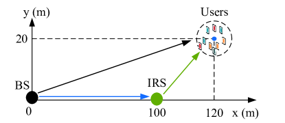
Figure 2: The simulated system setup.

We use IRS-Alg. 1 to represent Algorithm 1 and IRS-Alg. 2 to represent Algorithm 2. For comparison purposes, we show the performance of the scheme without IRS, in which the precoding matrix is also obtained by our proposed two algorithms, denoted as NIRS-Alg. 1 and NIRS-Alg. 2, respectively.

V-B Baseline Schemes

Due to the hardware limitation, it is practically difficult to realize the continuous phase shifts at each reflection element considered in this work. Hence, two baseline schemes with $2$ bit resolution are considered in the simulations to investigate the performance loss of using finite resolution reflection elements. Specifically, with optimal $\mathbf{e}^{o}$ generated by Algorithm 1 or Algorithm 2, the $m^{th}$ discrete phase shift can be obtained by

$$\theta_{m}^{o}=\arg\min_{\theta\in\mathcal{F}_{\theta}}|\exp\left\{j\angle\theta\right\}-e_{m}^{o}|,$$

where $\mathcal{F}_{\theta}=\{0,2\pi/B,...,2\pi(B-1)/B\}$ and $B=2^{2}$. Therefore, we call the two baseline schemes as IRS-Alg. 1, 2 bit and IRS-Alg. 2, 2 bit.

Besides, IRS is advocated as an energy-efficient device for assisting wireless communication. Hence, it is necessary to compare the performance of the IRS-based and the full-duplex amplify-and-forward (AF) relay-based multigroup multicast systems. To ensure a fair comparison with our proposed IRS-aided system, the Relay benchmark scheme, in which the relay is located at the same place of the IRS, has considered the same users’ locations and channel realizations. Then, the sum rate maximization problem for the joint design of the precoder $\mathbf{F}$ and the relay beamforming $\mathbf{W}$ is given by

$$\mathop{\max}\limits_{\mathbf{F},\mathbf{W}} \;\;\sum_{g=1}^{G}\min_{k\in\mathcal{K}_{g}}R_{k}^{relay}$$

$${\rm s.t.} \;\;||\mathbf{F}||_{F}^{2}\leq P_{\mathrm{T}}$$

$$\;\;||\mathbf{W}\mathbf{H_{\mathrm{dr}}}\mathbf{F}||_{F}^{2}+||\mathbf{W}||_{F}^{2}\sigma_{r}^{2}\leq P_{\mathrm{relay}},$$ (47)

where $R_{k}^{relay}$ is given by

$$\log_{2}\left(1+\frac{|(\mathbf{h}_{\mathrm{d},k}^{\mathrm{H}}+\mathbf{h}_{\mathrm{r},k}^{\mathrm{H}}\mathbf{W}\mathbf{H_{\mathrm{dr}}}){\bf f}_{g}|^{2}}{\sum_{i\neq g}^{G}|(\mathbf{h}_{\mathrm{d},k}^{\mathrm{H}}+\mathbf{h}_{\mathrm{r},k}^{\mathrm{H}}\mathbf{W}\mathbf{H_{\mathrm{dr}}}){\bf f}_{i}|^{2}+||\mathbf{h}_{\mathrm{r},k}^{\mathrm{H}}\mathbf{W}||_{2}^{2}\sigma_{r}^{2}+\sigma_{k}^{2}}\right).$$

Here, $P_{\mathrm{relay}}$ is the maximum available transmit power at the relay, $\sigma_{r}^{2}$ is the noise power received by the relay, and the digital relay beamforming $\mathbf{W}$ is assumed to be a diagonal matrix.

The AO method is adopted to solve the above problem. Basically, we extend the SCA method in [36] to alternately update each variable in Problem (47).

V-C Convergence of the Proposed Algorithms

Consider the fact of the nonconvexity of Problem (8), different initial points may result in different locally optimal solutions obtained by the our proposed algorithms. By testing 30 randomly channel realizations, Fig. 3 illustrates the impact of the initializations on the performance of the proposed algorithms. The initializations of IRS-Alg. 1 and IRS-Alg. 2 are: ${\bf F}$ is initialized by uniformly allocating maximum transmit power, ${\bf e}$ is initialized by setting each entry to 1. IRS-Alg. 1-EXH (IRS-Alg. 2-EXH) refers to the best initial point of 1000 random initial points for each channel realization. It can be seen that the sum rate of IRS-Alg. 1 (IRS-Alg. 2) is almost the same as that of IRS-Alg. 1-EXH (IRS-Alg. 2-EXH), implying that the simple uniform power allocation of ${\bf F}$ and all-one ${\bf e}$ is a good option for the initialization.

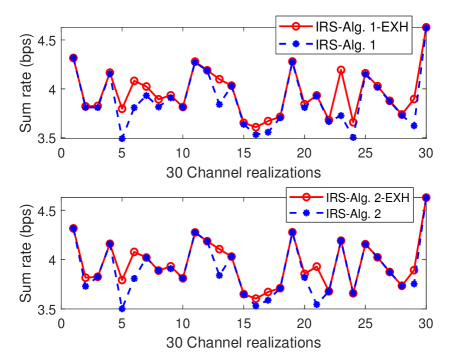
Figure 3: The performance comparison of different initialization, when $N=4$, $N=16$, $G=|\mathcal{K}_{g}|=2$ and $P_{\mathrm{T}}=15$ dBm.

In Fig. 4 investigates the convergence behaviour of various algorithms in terms of the iteration number and the CPU time when $P_{\mathrm{T}}=20$ dBm. Fig. 4(a) compares convergence speed in terms of the number of iterations. Only a small number of iterations are sufficient for Algorithm 1 to converge for both IRS and NIRS schemes. The reason is that the lower bound of the original objective function in (9) used in Algorithm 1 is tighter than those in (26) and (39) used in Algorithm 2. Although Algorithm 2 needs more iterations to converge, it has a fast convergence speed in terms of CPU time shown in Fig. 4(b). This is because in each iteration of Algorithm 2, there always exists closed-form solutions when designing precoding matrix and reflection coefficient vector. In addition, the optimal objective function values generated by both algorithms for IRS case and NIRS case are the same. Therefore, Algorithm 2 outperforms Algorithm 1 due to the fact that the former can generate the same gain with the latter while costing much less CPU running time

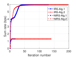
(a) The sum rate versus iteration number

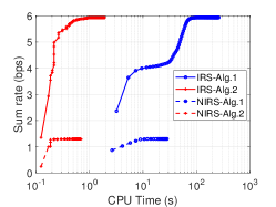
(b) The sum rate versus CPU time

Figure 4: The convergence behaviour of different algorithms, when $N=4$, $N=16$, $G=|\mathcal{K}_{g}|=2$ and $P_{\mathrm{T}}=20$ dBm.

V-D IRS vs AF relay Performance Comparison

Fig. 5 shows the sum rate, the energy efficiency, and the corresponding CPU running time under different maximum transmit power. The energy efficiency (bit/Hz/J) is defined as the ratio of the sum rate to the power consumption, i.e.,

$$EE=\frac{Sum\thinspace\thinspace Rate}{Power}\text{.}$$

In the relay-aided system, we set $P_{\mathrm{T}}=P_{\mathrm{relay}}$. The linear power consumption model is $Power=\eta(p_{\mathrm{T}}+p_{\mathrm{relay}})+NP_{t}+2MP_{r}$, where $p_{\mathrm{T}}$ and $p_{\mathrm{relay}}$ are the practical transmit power of the BS and the relay, respectively. Following [37], we set the reciprocal of the power amplifier efficiency as $\eta=1.2$ and the circuit power consumption of the active antennas at the BS and the relay as $P_{t}=P_{r}=200$ mW. In the IRS-aided system, we adopt $Power=\eta(p_{\mathrm{T}}+p_{\mathrm{relay}})+NP_{t}+MP_{IRS}$, where the circuit power consumption of the passive reflection elements is set as $P_{IRS}=5$ mW [38].

It can be seen in Fig. 5(a) that the IRS structure can obviously enhance the sum rate performance of the system without consuming additional transmit power, comparing with the system without the IRS structure. The performance loss of the ‘2 bit’ phase shifter generated by the proposed two algorithms is much small compared with the continuous phase shifter cases. However, the relay-aided system outperforms the IRS-aided one, which is reasonable due the fact that the relay can amplify and forward the received signals by using the relay transmit power $P_{\mathrm{relay}}$. The EE of the IRS-aided system shown in Fig. 5(b) is higher than the relay-aided one at high transmit power. The reason behind this is twofold. On the one hand, as $P_{\mathrm{T}}$ increases, the contribution of the relay transmit power $P_{\mathrm{relay}}$ to the system sum rate gain becomes less. On the other hand, the circuit power consumption of the relay is relatively high. Another observation from Fig. 5(b) is that the EE of the relay system decreases with the number of the active antennas deployed at the relay. From Fig. 5(c), we observe that Algorithm 1 is time-consuming and the time required is unacceptable when $P_{\mathrm{T}}$ increases. In addition, the computational complexity of the joint optimization of the precoder and the relay beamforming is much higher than the IRS case when $P_{\mathrm{T}}$ is less than 20 dBm due to the fact that relay power constraint is complex. Finally, all the results obtained from Fig. 5 verify the performance gains of the IRS-aided system in terms of the EE and complexity.

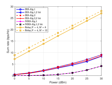
(a) Sum rate versus transmit power

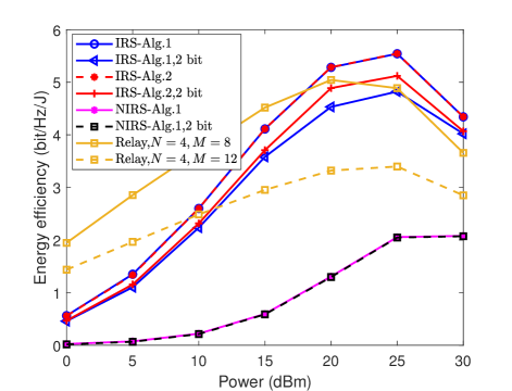
(b) Energy efficiency versus transmit power

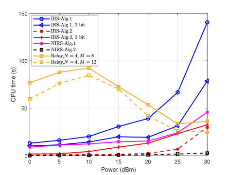
(c) CPU time versus transmit power

Figure 5: The sum rate, energy efficiency, and CPU time versus the transmit power, when $N=4$, $N=16$ and $G=|\mathcal{K}_{g}|=2$.

V-E IRS Performance Analysis

It is of practical significance to compare the communication performance of conventional large-scale antenna arrays deployed at the BS and large-scale passive elements deployed at the IRS, since IRS is regarded as an extension of massive MIMO antenna array. Fig. 6 illustrates the sum rate and the EE performance versus the numbers of antenna elements at the BS and reflection elements at the IRS when $P_{\mathrm{T}}=20$ dBm. It is observed from Fig. 6(a) that significant gains can be achieved by the IRS scheme over that without an IRS even when $M$ is as small as 4, and also that the spectral efficiency performance gains achieved by increasing the number of reflection elements are much higher than those achieved by increasing the number of transmit antennas. In addition, in Fig. 6(b), it is more energy-efficient to deploy an IRS with passive elements than installing active large-scale antenna array with energy-consuming radio frequency chains and power amplifiers. The trend of EE decreasing with the number of transmit antennas comes from the fact that the circut energy consumption of more antennas outweighs the system sum rate gain introduced by deploying more antennas. These simulation results demonstrate that IRS technology is superior to traditional massive MIMO in terms of spectral efficiency and energy efficiency.

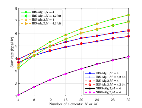
(a) Sum rate

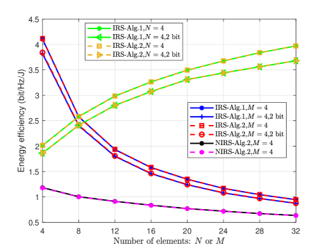
(b) Energy efficiency

Figure 6: The sum rate versus the numbers of reflection elements at the IRS $M$ or transmit antennas at the BS $N$, when $G=|\mathcal{K}_{g}|=2$ and $P_{\mathrm{T}}=20$ dBm.

The above simulation results show that Algorithm 2 requires less CPU time than Algorithm 1. Hence, we adopt Algorithm 2 to investigate the effect of an IRS on the performance of a multicast communication system. Fig. 7 illustrates the sum rate versus the number of users per group for various numbers of groups. It can be observed from this figure that the sum rate for all values of $G$ decreases with the increase of the number of users per group. The reason is that the data rate for each group is limited by the user with the worst channel condition. With the increase of the number of users per group, the channel gain for the worst user becomes smaller.

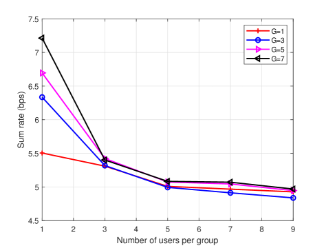
Figure 7: The sum rate versus the number of users per group, when $N=4$, $N=16$, and $P_{\mathrm{T}}=20$ dBm.

Fig. 7 compares the effects of two improvements on the performance limit, namely, increasing the number of antennas at the BS and the number of reflection elements at the IRS, respectively. When $|\mathcal{K}_{g}|=1$, the multicasting system reduces to a unitcasting system, in which the transmit antennas outperform the reflection elements in the aspect of suppressing multi-user interference. While when $|\mathcal{K}_{g}|=3$, the sum rate of the system increases slowly and tends to be stable with the increase of the number of multicasting groups for a given number of antenna/reflection elements.

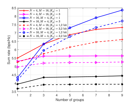
Figure 8: The sum rate versus the number of groups, when $P_{\mathrm{T}}=20$ dBm.

VI Conclusions

In this work, we have shown the performance benefits of introducing an IRS to the multigroup multicast systems. By carefully adjusting the reflection coefficients at the IRS, the signal reflected by the IRS can enhance the strength of the signal received by the user. We investigate the sum rate maximization problem by joint optimization of the precoding matrix at the BS and reflection coefficient vector at the IRS, while guaranteeing the transmit power constraint and the associated non-convex unit-modulus constraint at the IRS. Under the MM algorithm framework, we derive the concave lower bound of the original non-concave objective function, and then adopt alternating optimization method to update variables in an alternating manner. Furthermore, we proposed a low-complexity algorithm under the MM algorithm framework in which there exists closed-form solutions at each iteration. Our simulation results have demonstrated the significant spectral and energy efficiency enhancement of the IRS in multigroup multicast systems and that the proposed algorithm converges rapidly in terms of CPU time.

Appendix A The proof of Theorem 1

We perform some equivalent transformations of the rate expression (6) to show its hidden convexity, as follows

$$R_{k}\left(\mathbf{F},\mathbf{e}\right) =\log_{2}\left(1+\frac{|\mathbf{e}^{\mathrm{H}}\mathbf{H}_{k}{\bf f}_{g}|^{2}}{\sum_{i\neq g}^{G}|\mathbf{e}^{\mathrm{H}}\mathbf{H}_{k}{\bf f}_{i}|^{2}+\sigma_{k}^{2}}\right)$$

$$=\log_{2}\left(1+r_{k,-g}^{-1}|\mathbf{e}^{\mathrm{H}}\mathbf{H}_{k}{\bf f}_{g}|^{2}\right)$$

$$=-\log_{2}\left(1-\left(r_{k,-g}+|\mathbf{e}^{\mathrm{H}}\mathbf{H}_{k}{\bf f}_{g}|^{2}\right)^{-1}|\mathbf{e}^{\mathrm{H}}\mathbf{H}_{k}{\bf f}_{g}|^{2}\right)$$

$$=-\log_{2}\left(1-r_{k}^{-1}|t_{k}|^{2}\right),$$ (48)

where $t_{k}=\mathbf{e}^{\mathrm{H}}\mathbf{H}_{k}{\bf f}_{g}$, $r_{k}=r_{k,-g}+|t_{k}|^{2}$, and $r_{k,-g}=\sum_{i\neq g}^{G}|\mathbf{e}^{\mathrm{H}}\mathbf{H}_{k}{\bf f}_{i}|^{2}+\sigma_{k}^{2}$.

Denoting $R_{k}(t_{k},r_{k})$ as the last equation expression of $R_{k}\left(\mathbf{F},\mathbf{e}\right)$ in (48), $R_{k}(t_{k},r_{k})$ is jointly convex in $\{t_{k},r_{k}\}$ [39], thus its lower bound surrogate function could be obtained by the first-order approximation, e.g.,

$$R_{k}\left(t_{k},r_{k}\right)$$

$$\geq R_{k}\left(t_{k}^{n},r_{k}^{n}\right)+\frac{\partial R_{k}}{\partial t_{k}}|_{t_{k}=t_{k}^{n}}\left(t_{k}-t_{k}^{n}\right)$$

$$\ \ \ +\frac{\partial R_{k}}{\partial t_{k}^{*}}|_{t_{k}^{*}=t_{g}^{n,*}}\left(t_{k}^{*}-t_{k}^{n,*}\right)+\frac{\partial R_{k}}{\partial r_{k}}|_{r_{k}=r_{k}^{n}}\left(r_{k}-r_{k}^{n}\right)$$

$$=R_{k}\left(t_{k}^{n},r_{k}^{n}\right)+2\mathit{\mathrm{Re}}\left\{\frac{t_{k}^{n,*}(t_{k}-t_{k}^{n})}{r_{k}^{n}-|t_{k}^{n}|^{2}}\right\}-\frac{|t_{k}^{n}|^{2}(r_{k}-r_{k}^{n})}{r_{k}^{n}(r_{k}^{n}-|t_{k}^{n}|^{2})}$$

$$=R_{k}\left(t_{k}^{n},r_{k}^{n}\right)+2\mathit{\mathrm{Re}}\left\{\frac{t_{k}^{n,*}}{r_{k}^{n}-|t_{k}^{n}|^{2}}t_{k}\right\}$$

$$\thinspace\thinspace\thinspace\thinspace\thinspace\thinspace\thinspace\thinspace\thinspace\thinspace-\frac{|t_{k}^{n}|^{2}}{r_{k}^{n}(r_{k}^{n}-|t_{k}^{n}|^{2})}r_{k}-\frac{|t_{k}^{n}|^{2}}{r_{k}^{n}-|t_{k}^{n}|^{2}}.$$ (49)

Undo $t_{k}=\mathbf{e}^{\mathrm{H}}\mathbf{H}_{k}{\bf f}_{g}$, $t_{k}^{n}=(\mathbf{e}^{n})^{\mathrm{H}}\mathbf{H}_{k}{\bf f}_{g}^{n}$, $r_{k}=\sum_{i=1}^{G}|\mathbf{e}^{\mathrm{H}}\mathbf{H}_{k}{\bf f}_{i}|^{2}+\sigma_{k}^{2}$, and $r_{k}^{n}=\sum_{i=1}^{G}|(\mathbf{e}^{n})^{\mathrm{H}}\mathbf{H}_{k}{\bf f}_{i}^{n}|^{2}+\sigma_{k}^{2}$, and substitute them into the right hand side of the last equation in (49), we have

$$R_{k}\left(\mathbf{F},\mathbf{e}\right) \geq R_{k}\left(\mathbf{F}^{n},\mathbf{e}^{n}\right)+2\textrm{$\mathrm{Re}$}\left\{a_{k}\mathbf{e}^{\mathrm{H}}\mathbf{H}_{k}{\bf f}_{g}\right\}-\frac{|t_{k}^{n}|^{2}}{r_{k}^{n}-|t_{k}^{n}|^{2}}$$

$$\thinspace\thinspace\thinspace\thinspace\thinspace\thinspace\thinspace-b_{k}\sum_{i=1}^{G}|\mathbf{e}^{\mathrm{H}}\mathbf{H}_{k}{\bf f}_{i}|^{2}-b_{k}\sigma_{k}^{2}$$

$$=\textrm{const}_{k}+2\textrm{$\mathrm{Re}$}\left\{a_{k}\mathbf{e}^{\mathrm{H}}\mathbf{H}_{k}{\bf f}_{g}\right\}-b_{k}\sum_{i=1}^{G}|\mathbf{e}^{\mathrm{H}}\mathbf{H}_{k}{\bf f}_{i}|^{2}$$

$$=\widetilde{R}_{k}\left(\mathbf{F},\mathbf{e}\right).$$ (50)

Hence, the proof is complete.

Appendix B The proof of Theorem 1

The monotonic property of the objective function value sequence $\{F(\mathbf{F}^{n},\mathbf{e}^{n})\}$ of Algorithm 1 can be guaranteed by (18). In addition, the sequence $\{\mathbf{F}^{n},\mathbf{e}^{n}\}$ generated at each iteration of Algorithm 1 converges to a stable point as $n\rightarrow\infty$ because $\mathbf{F}^{n}$ and $\mathbf{e}^{n}$ are bounded in their feasible sets $\mathcal{S}_{F}$ and $\mathcal{S}_{e}$, respectively [40]. Denote by $\{\mathbf{F}^{o},\mathbf{e}^{o}\}$ the converged solution. In the following, we prove that $\{\mathbf{F}^{o},\mathbf{e}^{o}\}$ is the KKT point based on the fact that all the locally optimal solutions (including the globally optimal solution) of a nonconvex optimization problem should satisfy the KKT optimality conditions [29].

Firstly, the Lagrangian of Problem (13) is given by

$$\mathcal{L}\text{($\mathbf{F}$,$\bm{\gamma}$,$\bm{\lambda}^{(1)}$,$\lambda^{(2)}$)}$$

$$= \sum_{g=1}^{G}\gamma_{g}-\sum_{g=1}^{G}\sum_{k\in\mathcal{K}_{g}}\lambda_{k}^{(1)}(\gamma_{g}-\widetilde{R}_{k}\left(\mathbf{F},\mathbf{e}^{o}|\mathbf{F}^{o},\mathbf{e}^{o}\right))$$

$$-\lambda^{(2)}(\mathrm{Tr}\left[\mathbf{F}^{\mathrm{H}}\mathbf{F}\right]-P_{\mathrm{T}})$$

where $\bm{\lambda}^{(1)}=[\lambda_{1}^{(1)},...,\lambda_{K}^{(1)}]$ and $\lambda^{(2)}$ are the dual variables. Since $\mathbf{F}^{o}$ is the globally optimal solution of Problem (13), there must exist a $\bm{\lambda}^{(1),o}$ and $\lambda^{(2),o}$ satisfying the following partial KKT conditions:

$$\sum_{g=1}^{G}\sum_{k\in\mathcal{K}_{g}}\lambda_{k}^{(1),o}\nabla_{\mathbf{F}^{*}}\widetilde{R}_{k}\left(\mathbf{F},\mathbf{e}^{o}|\mathbf{F}^{o},\mathbf{e}^{o}\right)|_{\mathbf{F}=\mathbf{F}^{o}}-\lambda^{(2),o}\mathbf{F}^{o}=\mathbf{0},$$ (51)

$$\lambda_{k}^{(1),o}(\gamma_{g}-\widetilde{R}_{k}\left(\mathbf{F}^{o},\mathbf{e}^{o}|\mathbf{F}^{o},\mathbf{e}^{o}\right))=0,\forall k\in\mathcal{K}_{g},\forall g\in\mathcal{G},$$ (52)

$$\lambda^{(2),o}(\mathrm{Tr}\left[\mathbf{F}^{\mathrm{H},o}\mathbf{F}^{o}\right]-P_{\mathrm{T}})=0.$$ (53)

According to the conditions (A1) and (A3), we have

$$\widetilde{R}_{k}\left(\mathbf{F}^{o},\mathbf{e}^{o}|\mathbf{F}^{o},\mathbf{e}^{o}\right) =R_{k}\left(\mathbf{F}^{o},\mathbf{e}^{o}\right),$$ (54)

$$\nabla_{\mathbf{F}^{*}}\widetilde{R}_{k}\left(\mathbf{F},\mathbf{e}^{o}|\mathbf{F}^{o},\mathbf{e}^{o}\right)|_{\mathbf{F}=\mathbf{F}^{o}} =\nabla_{\mathbf{F}^{*}}R_{k}\left(\mathbf{F},\mathbf{e}^{o}\right)|_{\mathbf{F}=\mathbf{F}^{o}}.$$ (55)

By substituting (55) and (54) into (51) and (52) respectively, we arrive at

$$\sum_{g=1}^{G}\sum_{k\in\mathcal{K}_{g}}\lambda_{k}^{(1),o}\nabla_{\mathbf{F}^{*}}R_{k}\left(\mathbf{F},\mathbf{e}^{o}\right)|_{\mathbf{F}=\mathbf{F}^{o}}-\lambda^{(2),o}\mathbf{F}^{o}=\mathbf{0},$$ (56)

$$\lambda_{k}^{(1),o}(\gamma_{g}-R_{k}\left(\mathbf{F}^{o},\mathbf{e}^{o}\right))=0,\forall k\in\mathcal{K}_{g},\forall g\in\mathcal{G}.$$ (57)

Then, $\mathbf{e}^{o}$ is the locally optimal solution of Problem (16) and satisfies the following KKT conditions:

$$\sum_{g=1}^{G}\sum_{k\in\mathcal{K}_{g}}\xi_{k}^{(1),o}\nabla_{\mathbf{e}^{*}}\widetilde{R}_{k}\left(\mathbf{F}^{o},\mathbf{e}|\mathbf{F}^{o},\mathbf{e}^{o}\right)|_{\mathbf{e}=\mathbf{e}^{o}}-$$

$$\sum_{m=1}^{M}\xi_{m}^{(2),o}(\nabla_{\mathbf{e}^{*}}|e_{m}|)|_{\mathbf{e}=\mathbf{e}^{o}}-\xi_{M+1}^{(2),o}(\nabla_{\mathbf{e}^{*}}e_{M+1})|_{\mathbf{e}=\mathbf{e}^{o}}=\mathbf{0},$$ (58)

$$\xi_{k}^{(1),o}(\kappa_{g}-\widetilde{R}_{k}\left(\mathbf{F}^{o},\mathbf{e}^{o}|\mathbf{F}^{o},\mathbf{e}^{o}\right))=0,\forall k\in\mathcal{K}_{g},\forall g\in\mathcal{G},$$ (59)

$$\xi_{m}^{(2),o}(|e_{m}^{o}|-1)=0,1\leq m\leq M,\xi_{M+1}^{(2),o}(e_{M+1}^{o}-1)=0,$$ (60)

where $\bm{\xi}^{(1),o}=[\xi_{1}^{(1),o},...,\xi_{K}^{(1),o}]$ and $\xi^{(2),o}$ are the optimal Lagrange multipliers.

Furthermore, it can be readily checked that

$$\nabla_{\mathbf{e}^{*}}\widetilde{R}_{k}\left(\mathbf{F}^{o},\mathbf{e}|\mathbf{F}^{o},\mathbf{e}^{o}\right)|_{\mathbf{e}=\mathbf{e}^{o}} =\nabla_{\mathbf{e}^{*}}R_{k}\left(\mathbf{F}^{o},\mathbf{e}\right)|_{\mathbf{e}=\mathbf{e}^{o}}.$$ (61)

By substituting (61) into (58), we arrive at

$$\sum_{g=1}^{G}\sum_{k\in\mathcal{K}_{g}}\xi_{k}^{(1),o}\nabla_{\mathbf{e}^{*}}R_{k}\left(\mathbf{F}^{o},\mathbf{e}\right)|_{\mathbf{e}=\mathbf{e}^{o}}-\xi_{M+1}^{(2),o}(\nabla_{\mathbf{e}^{*}}e_{M+1})|_{\mathbf{e}=\mathbf{e}^{o}}$$

$$-\sum_{m=1}^{M}\xi_{m}^{(2),o}(\nabla_{\mathbf{e}^{*}}|e_{m}|)|_{\mathbf{e}=\mathbf{e}^{o}}=\mathbf{0},$$ (62)

Now, we move to Problem (8). The general equivalent problem of the max-min Problem (8) is given by

$$\mathop{\max}\limits_{\mathbf{F},\mathbf{e},\mathbf{r}} \;\;\sum_{g=1}^{G}r_{g}$$

$${\rm s.t.} \;\;\mathbf{F}\in\mathcal{S}_{F},\mathbf{e}\in\mathcal{S}_{e}$$

$$\;\;R_{k}\left(\mathbf{F},\mathbf{e}\right)\geq r_{g},\forall k\in\mathcal{K}_{g},\forall g\in\mathcal{G}.$$ (63)

where $\mathbf{r}=[r_{1},...,r_{G}]^{\mathrm{T}}$ are auxiliary variables. It can be readily verified that the set of equations (56), (62), (57), (53), and (60) constitute exactly the KKT conditions of Problem (63).

Hence, the proof is complete.

Appendix C The proof of Theorem 3

Since $f_{g}\left(\mathbf{F}\right)$ is twice differentiable and concave, we propose a quadratic surrogate function to minorize $f_{g}\left(\mathbf{F}\right)$, as follows

$$f_{g}(\mathbf{F}) \geq f_{g}(\mathbf{F}^{n})+2\textrm{$\mathrm{Re}$}\left\{\mathrm{\mathrm{Tr}}\left[\mathbf{D}_{g}^{\mathrm{H}}(\mathbf{F}-\mathbf{F}^{n})\right]\right\}$$

$$\thinspace\thinspace\thinspace\thinspace\thinspace\thinspace+\mathrm{Tr}\left[(\mathbf{F}-\mathbf{F}^{n})^{\mathrm{H}}\mathbf{M}_{g}(\mathbf{F}-\mathbf{F}^{n})\right]$$ (64)

where matrices $\mathbf{D}_{g}\in\mathbb{C}^{N\times N}$ and $\mathbf{M}_{g}\in\mathbb{C}^{N\times N}$ are determined to satisfy conditions (A1)-(A4).

Note that (A1) and (A4) are already satisfied. Then we prove that condition (A3) also holds. Let $\widetilde{\mathbf{F}}$ be a matrix belonging to $\mathcal{S}_{F}$. The directional derivative of the right hand side of (64) at $\mathbf{F}^{n}$ with direction $\widetilde{\mathbf{F}}-\mathbf{F}^{n}$ is given by:

$$2\textrm{Re}\left\{\mathrm{\mathrm{Tr}}\left[\mathbf{D}_{g}^{\mathrm{H}}(\widetilde{\mathbf{F}}-\mathbf{F}^{n})\right]\right\}.$$ (65)

The directional derivative of $f_{g}(\mathbf{F})$ is

$$2\textrm{{$\mathrm{Re}$}}\left\{\mathrm{\mathrm{Tr}}\left[\sum_{k\in\mathcal{K}_{g}}g_{k}(\mathbf{F}^{n})(\mathbf{C}_{k}^{\mathrm{H}}-(\mathbf{F}^{n})^{\mathrm{H}}\mathbf{B}_{k})(\widetilde{\mathbf{F}}-\mathbf{F}^{n})\right]\right\},$$ (66)

where $g_{k}(\mathbf{F}^{n})$ is defined in (28).

In order to satisfy condition (A3), the two directional derivatives (65) and (66) must be equal, which means

$$\mathbf{D}_{g}=\sum_{k\in\mathcal{K}_{g}}g_{k}(\mathbf{F}^{n})(\mathbf{C}_{k}-\mathbf{B}_{k}^{\mathrm{H}}\mathbf{F}^{n}).$$ (67)

Now we proceed to prove that condition (A2) also holds. If surrogate function $\widetilde{f}_{g}(\mathbf{F}|\mathbf{F}^{n})$ is a lower bound for each linear cut in any direction, condition (A2) could be satisfied. Let $\mathbf{F}=\mathbf{F}^{n}+\gamma(\widetilde{\mathbf{F}}-\mathbf{F}^{n}),\forall\gamma\in[0,1]$. Then, it suffices to show

$$f_{g}(\mathbf{F}^{n}+\gamma(\widetilde{\mathbf{F}}-\mathbf{F}^{n})) \geq f_{g}(\mathbf{F}^{n})+2\gamma\textrm{$\mathrm{Re}$}\left\{\mathrm{\mathrm{Tr}}\left[\mathbf{D}_{g}^{\mathrm{H}}(\widetilde{\mathbf{F}}-\mathbf{F}^{n})\right]\right\}$$

$$+\gamma^{2} \mathrm{\mathrm{Tr}}\left[(\widetilde{\mathbf{F}}-\mathbf{F}^{n})^{\mathrm{H}}\mathbf{M}_{g}(\widetilde{\mathbf{F}}-\mathbf{F}^{n})\right],$$ (68)

Let us define $L_{g}(\gamma)=f_{g}(\mathbf{F}^{n}+\gamma(\widetilde{\mathbf{F}}-\mathbf{F}^{n})),$and $l_{k}(\gamma)=\widetilde{R}_{k}(\mathbf{F}^{n}+\gamma(\widetilde{\mathbf{F}}-\mathbf{F}^{n})).$ Now, a sufficient condition for (68) to hold is that the second derivative of the right hand side of (68) is lower than or equal to the second derivative of the left hand side of (68) for $\forall\gamma\in[0,1]$ and $\forall\widetilde{\mathbf{F}},\forall\mathbf{F}^{n}\in\mathcal{S}_{F}$, which is formulated as follows

$$\frac{\partial^{2}L_{g}(\gamma)}{\partial\gamma^{2}}\geq 2\mathrm{\mathrm{Tr}}\left[(\widetilde{\mathbf{F}}-\mathbf{F}^{n})^{\mathrm{H}}\mathbf{M}_{g}(\widetilde{\mathbf{F}}-\mathbf{F}^{n})\right].$$ (69)

In order to calculate the left hand side of (69), we first calculate the first-order derivative, as follows

$$\frac{\partial L_{g}(\gamma)}{\partial\gamma} =\sum_{k\in\mathcal{K}_{g}}g_{k}(\gamma)\nabla_{\gamma}l_{k}(\gamma),$$ (70)

where

$$g_{k}(\gamma) =\frac{\mathrm{exp}\left\{-\mu_{g}l_{k}(\gamma)\right\}}{\sum_{k\in\mathcal{K}_{g}}\mathrm{exp}\left\{-\mu_{g}l_{k}(\gamma)\right\}},k\in\mathcal{K}_{g},$$

$$\nabla_{\gamma}l_{k}(\gamma) =2\textrm{$\mathrm{Re}$}\Bigl{\{}\mathrm{\mathrm{Tr}}\left[\mathbf{C}_{k}^{\mathrm{H}}(\widetilde{\mathbf{F}}-\mathbf{F}^{n})\right]$$

$$\ \ \ -\mathrm{Tr}\left[(\mathbf{F}^{n}+\gamma(\widetilde{\mathbf{F}}-\mathbf{F}^{n}))^{\mathrm{H}}\mathbf{B}_{k}(\widetilde{\mathbf{F}}-\mathbf{F}^{n})\right]\Bigr{\}}$$

$$=2\textrm{$\mathrm{Re}$}\left\{\mathrm{\mathrm{Tr}}\left[\mathbf{Q}_{k}^{\mathrm{H}}(\widetilde{\mathbf{F}}-\mathbf{F}^{n})\right]\right\}$$

$$=2\textrm{$\mathrm{Re}$}\left\{\mathbf{q}_{k}^{\mathrm{H}}\mathbf{f}\right\},$$

$$\mathbf{Q}_{k}^{\mathrm{H}} =\mathbf{C}_{k}^{\mathrm{H}}-(\mathbf{F}^{n}+\gamma(\widetilde{\mathbf{F}}-\mathbf{F}^{n}))^{\mathrm{H}}\mathbf{B}_{k},$$

$$\mathbf{q}_{k} =\mathrm{vec}(\mathbf{Q}_{k}),$$

$$\mathbf{f} =\mathrm{vec}(\widetilde{\mathbf{F}}-\mathbf{F}^{n}),$$

Then, the second-order derivative is derived as

$$\frac{\partial^{2}L_{g}(\gamma)}{\partial\gamma^{2}}$$

$$=\sum_{k\in\mathcal{K}_{g}}\left(g_{k}(\gamma)\nabla_{\gamma}^{2}l_{k}(\gamma)-\mu_{g}g_{k}(\gamma)\nabla_{\gamma}l_{k}(\gamma)\left(\nabla_{\gamma}l_{k}(\gamma)\right)^{\mathrm{T}}\right)$$

$$+\mu_{g}\left(\sum_{k\in\mathcal{K}_{g}}g_{k}(\gamma)\nabla_{\gamma}l_{k}(\gamma)\right)\left(\sum_{k\in\mathcal{K}_{g}}g_{k}(\gamma)\nabla_{\gamma}l_{k}(\gamma)\right)^{\mathrm{T}},$$ (71)

where

$$\nabla_{\gamma}^{2}l_{k}(\gamma) =-2\mathrm{\mathrm{Tr}}\left[(\widetilde{\mathbf{F}}-\mathbf{F}^{n})^{\mathrm{H}}\mathbf{B}_{k}(\widetilde{\mathbf{F}}-\mathbf{F}^{n})\right]$$

$$=-2\mathbf{f}{}^{\mathrm{H}}(\mathbf{I}\otimes\mathbf{B}_{k})\mathbf{f}.$$

We reformulate $\frac{\partial^{2}L_{g}(\gamma)}{\partial\gamma^{2}}$ in (71) into a quadratic form of $\mathbf{f}$, as follows

$$\frac{\partial^{2}L_{g}(\gamma)}{\partial\gamma^{2}} =\left[\begin{array}[]{cc}\mathbf{f}{}^{\mathrm{H}}&\mathbf{f}{}^{\mathrm{T}}\end{array}\right]\bm{\Phi}\left[\begin{array}[]{c}\mathbf{f}\\ \mathbf{f}{}^{*}\end{array}\right],$$

where $\bm{\Phi}$ is given in (82).

$$\bm{\Phi}_{g} =\sum_{k\in\mathcal{K}_{g}}\left(g_{k}(\gamma)\left[\begin{array}[]{cc}-\mathbf{I}\otimes\mathbf{B}_{k}&\mathbf{0}\\ \mathbf{0}&-\mathbf{I}\otimes\mathbf{B}_{k}^{\mathrm{T}}\end{array}\right]-\mu_{g}g_{k}(\gamma)\left[\begin{array}[]{c}\mathbf{q}_{k}\\ \mathbf{q}_{k}^{\mathrm{*}}\end{array}\right]\left[\begin{array}[]{c}\mathbf{q}_{k}\\ \mathbf{q}_{k}^{\mathrm{*}}\end{array}\right]^{\mathrm{H}}\right)+\mu_{g}\left[\begin{array}[]{c}\sum_{k\in\mathcal{K}_{g}}g_{k}(\gamma)\mathbf{q}_{k}\\ \sum_{k\in\mathcal{K}_{g}}g_{k}(\gamma)\mathbf{q}_{k}^{\mathrm{*}}\end{array}\right]\left[\begin{array}[]{c}\sum_{k\in\mathcal{K}_{g}}g_{k}(\gamma)\mathbf{q}_{k}\\ \sum_{k\in\mathcal{K}_{g}}g_{k}(\gamma)\mathbf{q}_{k}^{\mathrm{*}}\end{array}\right]^{\mathrm{H}}\text{.}$$ (82)

 

We also manipulate the right hand side of (69) into a quadratic form of $\mathbf{f}$ by using vectorization operation $\mathrm{Tr}[\mathbf{A}^{\mathrm{T}}\mathbf{B}\mathbf{C}]=\mathrm{vec}^{\mathrm{T}}(\mathbf{A})(\mathbf{I}\otimes\mathbf{B})\mathrm{vec}(\mathbf{C})$ [41], as follows

$$2\mathrm{\mathrm{Tr}}\left[(\widetilde{\mathbf{F}}-\mathbf{F}^{n})^{\mathrm{H}}\mathbf{M}_{g}(\widetilde{\mathbf{F}}-\mathbf{F}^{n})\right]$$

$$=\left[\begin{array}[]{cc}\mathbf{f}{}^{\mathrm{H}}&\mathbf{f}{}^{\mathrm{T}}\end{array}\right]\left[\begin{array}[]{cc}\mathbf{I}\otimes\mathbf{M}_{g}&\mathbf{0}\\ \mathbf{0}&\mathbf{I}\otimes\mathbf{M}_{g}^{\mathrm{T}}\end{array}\right]\left[\begin{array}[]{c}\mathbf{f}\\ \mathbf{f}{}^{*}\end{array}\right].$$

Then, (69) is equivalent to

$$\left[\begin{array}[]{cc}\mathbf{f}{}^{\mathrm{H}}&\mathbf{f}{}^{\mathrm{T}}\end{array}\right]\bm{\Phi}_{g}\left[\begin{array}[]{c}\mathbf{f}\\ \mathbf{f}{}^{*}\end{array}\right]$$

$$\geq\left[\begin{array}[]{cc}\mathbf{f}{}^{\mathrm{H}}&\mathbf{f}{}^{\mathrm{T}}\end{array}\right]\left[\begin{array}[]{cc}\mathbf{I}\otimes\mathbf{M}_{g}&\mathbf{0}\\ \mathbf{0}&\mathbf{I}\otimes\mathbf{M}_{g}^{\mathrm{T}}\end{array}\right]\left[\begin{array}[]{c}\mathbf{f}\\ \mathbf{f}{}^{*}\end{array}\right],$$

where we need to find an $\mathbf{M}_{g}$ that satisfies

$$\bm{\Phi}_{g}\succeq\left[\begin{array}[]{cc}\mathbf{I}\otimes\mathbf{M}_{g}&\mathbf{0}\\ \mathbf{0}&\mathbf{I}\otimes\mathbf{M}_{g}^{\mathrm{T}}\end{array}\right].$$

For convenience, we choose $\mathbf{M}_{g}=\alpha_{g}\mathbf{I}=\lambda_{\mathrm{min}}\left(\bm{\Phi}_{g}\right)\mathbf{I}$. Finally, (64) is equivalent to

$$f_{g}(\mathbf{F}) \geq f_{g}(\mathbf{F}^{n})+2\textrm{$\mathrm{Re}$}\left\{\mathrm{Tr}\left[\mathbf{D}_{g}^{\mathrm{H}}(\mathbf{F}-\mathbf{F}^{n})\right]\right\}$$

$$\thinspace\thinspace\thinspace\thinspace\thinspace\thinspace+\alpha_{g}\mathrm{\mathrm{Tr}}\left[(\mathbf{F}-\mathbf{F}^{n})^{\mathrm{H}}(\mathbf{F}-\mathbf{F}^{n})\right]$$

$$=2\textrm{$\mathrm{Re}$}\left\{\mathrm{\mathrm{Tr}}\left[\mathbf{U}_{g}^{\mathrm{H}}\mathbf{F}\right]\right\}+\alpha_{g}\mathrm{Tr}\left[\mathbf{F}^{\mathrm{H}}\mathbf{F}\right]+\textrm{consF}_{g}$$ (83)

where $\mathbf{U}_{g}$ and $\textrm{consF}_{g}$ are given in (27) and (31), respectively. $\alpha_{g}$ in (29) is difficult to obtain for the complex expression of $\bm{\Phi}_{g}$. In the following, we proceed to obtain the value of $\alpha_{g}$.

The following inequalities and equalities will be used later:

(B1): [41] $\mathbf{A}$ and $\mathbf{B}$ are Hermitian matrices: $\lambda_{\mathrm{min}}(\mathbf{A})+\lambda_{\mathrm{min}}(\mathbf{B})\leq\lambda_{\mathrm{min}}(\mathbf{A}+\mathbf{B}).$

(B2): [41] $\mathbf{A}$ is rank one: $\lambda_{\mathrm{max}}(\mathbf{A})=\mathrm{\mathrm{Tr}}\left[\mathbf{A}\right],\lambda_{\mathrm{min}}(\mathbf{A})=0$.

(B3): (Theorem 30 in [42]) $a_{k}$ and $b_{k}$ are positive: $\sum_{k=1}^{K}a_{k}b_{k}\leq\mathrm{max}_{k=1}^{K}\left\{b_{k}\right\}$, if $\sum_{k=1}^{K}a_{k}=1$.

(B4): [41] $\mathbf{A}$ is positive semidifinite with maximum eigenvalue $\lambda_{\mathrm{max}}(\mathbf{A})$ and $\mathbf{B}$ is positive semidifinite: $\mathrm{\mathrm{Tr}}\left[\mathbf{A}\mathbf{B}\right]\leq\lambda_{\mathrm{max}}(\mathbf{A})\mathrm{\mathrm{Tr}}\left[\mathbf{B}\right]$.

$\bm{\Phi}_{g}$ is complex and cannot be determined by a constant, thus we use (A1)-(A4) to find its lower bound shown in (96).

$$\lambda_{\mathrm{min}}\left(\bm{\Phi}_{g}\right) \overset{\mathrm{(B1)}}{\geq}-\sum_{k\in\mathcal{K}_{g}}g_{k}(\gamma)\lambda_{\mathrm{max}}\left(\left[\begin{array}[]{cc}\mathbf{I}\otimes\mathbf{B}_{k}&\mathbf{0}\\ \mathbf{0}&\mathbf{I}\otimes\mathbf{B}_{k}^{\mathrm{T}}\end{array}\right]\right)-\mu_{g}\sum_{k\in\mathcal{K}_{g}}g_{k}(\gamma)\lambda_{\mathrm{max}}\left(\left[\begin{array}[]{c}\mathbf{q}_{k}\\ \mathbf{q}_{k}^{\mathrm{*}}\end{array}\right]\left[\begin{array}[]{c}\mathbf{q}_{k}\\ \mathbf{q}_{k}^{\mathrm{*}}\end{array}\right]^{\mathrm{H}}\right)$$ (90)

$$~{}~{}~{}~{}~{}+\lambda_{\mathrm{min}}\left(\mu_{g}\left[\begin{array}[]{c}\sum_{k\in\mathcal{K}_{g}}g_{k}(\gamma)\mathbf{q}_{k}\\ \sum_{k\in\mathcal{K}_{g}}g_{k}(\gamma)\mathbf{q}_{k}^{\mathrm{*}}\end{array}\right]\left[\begin{array}[]{c}\sum_{k\in\mathcal{K}_{g}}g_{k}(\gamma)\mathbf{q}_{k}\\ \sum_{k\in\mathcal{K}_{g}}g_{k}(\gamma)\mathbf{q}_{k}^{\mathrm{*}}\end{array}\right]^{\mathrm{H}}\right)$$ (95)

$$\overset{\mathrm{(B2)}}{=}-\sum_{k\in\mathcal{K}_{g}}g_{k}(\gamma)\lambda_{\mathrm{max}}(\mathbf{B}_{k})-2\mu_{g}\sum_{k\in\mathcal{K}_{g}}g_{k}(\gamma)\mathbf{q}_{k}^{\mathrm{H}}\mathbf{q}_{k}$$

$$\overset{\mathrm{(B2)}}{=}-\sum_{k\in\mathcal{K}_{g}}b_{k}g_{k}(\gamma)\mathbf{e}^{\mathrm{H}}\mathbf{H}_{k}\mathbf{H}_{k}^{\mathrm{H}}\mathbf{e}-2\mu_{g}\sum_{k\in\mathcal{K}_{g}}g_{k}(\gamma)\mathbf{q}_{k}^{\mathrm{H}}\mathbf{q}_{k}$$

$$\overset{\mathrm{(B3)}}{\geq}-\mathrm{max}_{k\in\mathcal{K}_{g}}\left\{b_{k}\mathbf{e}^{\mathrm{H}}\mathbf{H}_{k}\mathbf{H}_{k}^{\mathrm{H}}\mathbf{e}\right\}-2\mu_{g}\mathrm{max}_{k\in\mathcal{K}_{g}}\left\{||\mathbf{q}_{k}||_{2}^{2}\right\}$$

$$=-\mathrm{max}_{k\in\mathcal{K}_{g}}\left\{b_{k}\mathbf{e}^{\mathrm{H}}\mathbf{H}_{k}\mathbf{H}_{k}^{\mathrm{H}}\mathbf{e}\right\}-2\mu_{g}\mathrm{max}_{k\in\mathcal{K}_{g}}\left\{||\mathbf{Q}_{k}||_{F}^{2}\right\}.$$ (96)

 

Recall that $\mathbf{F}=\mathbf{F}^{n}+\gamma(\widetilde{\mathbf{F}}-\mathbf{F}^{n}),\forall\gamma\in[0,1]$, therefore $||\mathbf{F}^{n}+\gamma(\widetilde{\mathbf{F}}-\mathbf{F}^{n})||_{F}^{2}\leq P_{\mathrm{T}}$. By using (A4), the last term in the right hand side of the last equation of (96) satisfies inequality (97) as

$$||\mathbf{Q}_{k}||_{F}^{2} =||\mathbf{C}_{k}-\mathbf{B}_{k}^{\mathrm{H}}(\mathbf{F}^{n}+\gamma(\widetilde{\mathbf{F}}-\mathbf{F}^{n}))||_{F}^{2}$$

$$=||(\mathbf{F}^{n}+\gamma(\widetilde{\mathbf{F}}-\mathbf{F}^{n}))^{\mathrm{H}}\mathbf{B}_{k}||_{F}^{2}+||\mathbf{C}_{k}||_{F}^{2}$$

$$\thinspace\thinspace\thinspace\thinspace\thinspace\thinspace-2\textrm{$\mathrm{Re}$}\left\{\mathrm{Tr}\left[\mathbf{C}_{k}^{\mathrm{H}}\mathbf{B}_{k}^{\mathrm{H}}(\mathbf{F}^{n}+\gamma(\widetilde{\mathbf{F}}-\mathbf{F}^{n}))\right]\right\}$$

$$\overset{\mathrm{(B4)}}{\leq}\lambda_{\mathrm{max}}(\mathbf{B}_{k}\mathbf{B}_{k}^{\mathrm{H}})||\mathbf{F}^{n}+\gamma(\widetilde{\mathbf{F}}-\mathbf{F}^{n})||_{F}^{2}+||\mathbf{C}_{k}||_{F}^{2}$$

$$\thinspace\thinspace\thinspace\thinspace\thinspace\thinspace\thinspace-2\textrm{$\mathrm{Re}$}\left\{\mathrm{\mathrm{Tr}}\left[\mathbf{C}_{k}^{\mathrm{H}}\mathbf{B}_{k}^{\mathrm{H}}(\mathbf{F}^{n}+\gamma(\widetilde{\mathbf{F}}-\mathbf{F}^{n}))\right]\right\}$$

$$\leq P_{\mathrm{T}}\lambda_{\mathrm{max}}(\mathbf{B}_{k}\mathbf{B}_{k}^{\mathrm{H}})+||\mathbf{C}_{k}||_{F}^{2}+2\sqrt{P_{\mathrm{T}}}||\mathbf{B}_{k}\mathbf{C}_{k}||_{F}$$

$$=P_{\mathrm{T}}b_{k}^{2}|\mathbf{e}^{\mathrm{H}}\mathbf{H}_{k}\mathbf{H}_{k}^{\mathrm{H}}\mathbf{e}|^{2}+||\mathbf{C}_{k}||_{F}^{2}+2\sqrt{P_{\mathrm{T}}}||\mathbf{B}_{k}\mathbf{C}_{k}||_{F}.$$ (97)

The third term in the right hand side of the last inequality of (97) is the optimal objective value of the following Problem (98) which has a closed-form solution.

$$\mathop{\mathrm{min}}\limits_{\mathbf{X}} \;\;2\textrm{Re}\left\{\mathrm{\mathrm{Tr}}\left[\mathbf{C}_{k}^{\mathrm{H}}\mathbf{B}_{k}^{\mathrm{H}}\mathbf{X}\right]\right\}$$

$${\rm s.t.} \thinspace\thinspace\thinspace\thinspace\mathrm{\mathrm{Tr}}\left[\mathbf{X}^{\mathrm{H}}\mathbf{X}\right]\leq P_{\mathrm{T}}.$$ (98)

Finally, combining (96) with (97), we arrive at (29). Hence, the proof is complete.

Appendix D The proof of Theorem 4

Since $f_{g}\left(\mathbf{e}\right)$ is twice differentiable and concave, we minorize $f_{g}\left(\mathbf{e}\right)$ at $\mathbf{e}^{n}$ with a quadratic function, as follows

$$f_{g}(\mathbf{e})\geq f_{g}(\mathbf{e}^{n})+2\textrm{$\mathrm{Re}$}\left\{\mathbf{d}_{g}^{\mathrm{H}}(\mathbf{e}-\mathbf{e}^{n})\right\}$$

$$+(\mathbf{e}-\mathbf{e}^{n})^{\mathrm{H}}\mathbf{N}_{g}(\mathbf{e}-\mathbf{e}^{n}),$$ (99)

where vectors $\mathbf{d}_{g}\in\mathbb{C}^{M\times 1}$ and matrices $\mathbf{N}_{g}\in\mathbb{C}^{M\times M}$ are determined to satisfy conditions (A1)-(A4).

Obviously, (A1) and (A4) are already satisfied. In order to satisfy condition (A3), the directional derivatives of $f_{g}(\mathbf{e})$ and the right hand side of (99) must be equal, yielding

$$\mathbf{d}_{g}=\sum_{k\in\mathcal{K}_{g}}g_{k}(\mathbf{e}^{n})(\mathbf{a}_{k}-\mathbf{A}_{k}^{\mathrm{H}}\mathbf{e}^{n}),$$ (100)

where $g_{k}(\mathbf{e}^{n})$ is defined in (41).

Let $\mathbf{e}=\mathbf{e}^{n}+\gamma(\widetilde{\mathbf{e}}-\mathbf{e}^{n}),\forall\gamma\in[0,1]$. In order to satisfy condition (A2), it suffices to show

$$f_{g}(\mathbf{e}^{n}+\gamma(\widetilde{\mathbf{e}}-\mathbf{e}^{n})) \geq f_{g}(\mathbf{e}^{n})+2\gamma\textrm{$\mathrm{Re}$}\left\{\mathbf{d}_{g}^{\mathrm{H}}(\widetilde{\mathbf{e}}-\mathbf{e}^{n})\right\}$$

$$+\gamma^{2}(\widetilde{\mathbf{e}}-\mathbf{e}^{n})^{\mathrm{H}}\mathbf{N}_{g}(\widetilde{\mathbf{e}}-\mathbf{e}^{n}).$$ (101)

Then, we need to calculate the second-order derivatives of the left hand side and the right hand side of (101), and make the latter one lower than or equal to the former for $\forall\gamma\in[0,1]$ and $\forall\widetilde{\mathbf{e}},\forall\mathbf{e}^{n}\in\mathcal{S}_{e}$.

The second-order derivative of the left hand side of (101) is given by

$$\frac{\partial^{2}L_{g}(\gamma)}{\partial\gamma^{2}} =\left[\begin{array}[]{cc}\mathbf{t}{}^{\mathrm{H}}&\mathbf{t}{}^{\mathrm{T}}\end{array}\right]\bm{\Psi}_{g}\left[\begin{array}[]{c}\mathbf{t}\\ \mathbf{t}{}^{*}\end{array}\right],$$ (105)

with $\mathbf{t}=\widetilde{\mathbf{e}}-\mathbf{e}^{n}$. $\bm{\Psi}_{g}$ is shown in (116) where

$$\bm{\Psi}_{g}=\sum_{k\in\mathcal{K}_{g}}\left(g_{k}(\gamma)\left[\begin{array}[]{cc}-\mathbf{A}_{k}&0\\ \mathbf{0}&-\mathbf{A}_{k}^{\mathrm{T}}\end{array}\right]-\mu_{g}g_{k}(\gamma)\left[\begin{array}[]{c}\mathbf{q}_{k}\\ \mathbf{q}_{k}^{\mathrm{*}}\end{array}\right]\left[\begin{array}[]{c}\mathbf{q}_{k}\\ \mathbf{q}_{k}^{\mathrm{*}}\end{array}\right]^{\mathrm{H}}\right)+\mu_{g}\left[\begin{array}[]{c}\sum_{k\in\mathcal{K}_{g}}g_{k}(\gamma)\mathbf{q}_{k}\\ \sum_{k\in\mathcal{K}_{g}}g_{k}(\gamma)\mathbf{q}_{k}^{\mathrm{*}}\end{array}\right]\left[\begin{array}[]{c}\sum_{k\in\mathcal{K}_{g}}g_{k}(\gamma)\mathbf{q}_{k}\\ \sum_{k\in\mathcal{K}_{g}}g_{k}(\gamma)\mathbf{q}_{k}^{\mathrm{*}}\end{array}\right]^{\mathrm{H}},$$ (116)

 

$$\mathbf{q}_{k} =\mathbf{a}_{k}-\mathbf{A}_{k}^{\mathrm{H}}(\mathbf{e}^{n}+\gamma(\widetilde{\mathbf{e}}-\mathbf{e}^{n}))$$ (117)

$$g_{k}(\gamma) =\frac{\mathrm{exp}\left\{-\mu_{g}l_{k}(\gamma)\right\}}{\sum_{k\in\mathcal{K}_{g}}\mathrm{exp}\left\{-\mu_{g}l_{k}(\gamma)\right\}},k\in\mathcal{K}_{g}$$ (118)

The second-order derivative of the right hand side of (101) is

$$2(\widetilde{\mathbf{e}}-\mathbf{e}^{n})^{\mathrm{H}}\mathbf{N}_{g}(\widetilde{\mathbf{e}}-\mathbf{e}^{n})$$

$$= \left[\begin{array}[]{cc}\mathbf{t}{}^{\mathrm{H}}&\mathbf{t}{}^{\mathrm{T}}\end{array}\right]\left[\begin{array}[]{cc}\mathbf{I}\otimes\mathbf{N}_{g}&\mathbf{0}\\ \mathbf{0}&\mathbf{I}\otimes\mathbf{N}_{g}^{\mathrm{T}}\end{array}\right]\left[\begin{array}[]{c}\mathbf{t}\\ \mathbf{t}{}^{*}\end{array}\right].$$ (124)

Combining (105) with (124), $\mathbf{N}_{g}$ must satisfy

$$\bm{\Psi}_{g}\succeq\left[\begin{array}[]{cc}\mathbf{I}\otimes\mathbf{N}_{g}&\mathbf{0}\\ \mathbf{0}&\mathbf{I}\otimes\mathbf{N}_{g}^{\mathrm{T}}\end{array}\right].$$

For simplicity, we choose $\mathbf{N}_{g}=\beta_{g}\mathbf{I}=\lambda_{\mathrm{min}}(\bm{\Psi}_{g})\mathbf{I}$. Eventually, (99) is equivalent to

$$f_{g}(\mathbf{e}) \geq f_{g}(\mathbf{e}^{n})+2\textrm{$\mathrm{Re}$}\left\{\mathbf{d}_{g}^{\mathrm{H}}(\mathbf{e}-\mathbf{e}^{n})\right\}+\beta_{g}(\mathbf{e}-\mathbf{e}^{n})^{\mathrm{H}}(\mathbf{e}-\mathbf{e}^{n})$$

$$=2\textrm{$\mathrm{Re}$}\left\{\mathbf{u}_{g}^{\mathrm{H}}\mathbf{e}\right\}+\textrm{consE}_{g},$$ (125)

where $\mathbf{u}_{g}$, $\beta_{g}$, and $\textrm{consE}_{g}$ are given in (40), (42), and (44), respectively. The last equation of (125) is from the unit-modulus constraints, i.e., $\mathbf{e}^{\mathrm{H}}\mathbf{e}=(\mathbf{e}^{n})^{\mathrm{H}}\mathbf{e}^{n}=M+1$. The method to get the value of $\beta_{g}$ is similar as $\alpha_{g}$, so we omit it here. Hence, the proof is complete.

Appendix E The proof of Theorem 5

Let us denote the converged solution of Problem (24) by $\{\mathbf{F}^{o},\mathbf{e}^{o}\}$. In the following, we prove that $\{\mathbf{F}^{o},\mathbf{e}^{o}\}$ satisfies the KKT conditions of Problem (24).

Firstly, since $\mathbf{F}^{o}$ is the globally optimal solution of Problem (32), the KKT conditions of the Lagrangian in (33) of Problem (32) is given by

$$\sum_{g=1}^{G}\nabla_{\mathbf{F}^{*}}\widetilde{f}_{g}(\mathbf{F}|\mathbf{F}^{n})|_{\mathbf{F}=\mathbf{F}^{o}}-\tau^{o}\mathbf{F}^{o}=\mathbf{0},$$ (126)

$$\tau^{o}(\mathrm{Tr}\left[\mathbf{F}^{\mathrm{H},o}\mathbf{F}^{o}\right]-P_{\mathrm{T}})=0,$$ (127)

where $\tau^{o}$ is the optimal Lagrange multiplier. According to the condition (A3), we have

$$\nabla_{\mathbf{F}^{*}}\widetilde{f}_{g}(\mathbf{F}|\mathbf{F}^{n})|_{\mathbf{F}=\mathbf{F}^{o}} =\nabla_{\mathbf{F}^{*}}f_{g}\left(\mathbf{F},\mathbf{e}^{o}\right)|_{\mathbf{F}=\mathbf{F}^{o}}.$$ (128)

By substituting (128) into (126), we arrive at

$$\sum_{g=1}^{G}\nabla_{\mathbf{F}^{*}}f_{g}\left(\mathbf{F},\mathbf{e}^{o}\right)|_{\mathbf{F}=\mathbf{F}^{o}}-\tau^{o}\mathbf{F}^{o}=\mathbf{0},$$ (129)

Then, since $\mathbf{e}^{o}$ is the locally optimal solution of Problem (45), it is readily to obtain the following KKT conditions:

$$\sum_{g=1}^{G}\nabla_{\mathbf{e}^{*}}f_{g}\left(\mathbf{F}^{o},\mathbf{e}\right)|_{\mathbf{e}=\mathbf{e}^{o}}-\sum_{m=1}^{M}\tau_{m}^{(2),o}(\nabla_{\mathbf{e}^{*}}|e_{m}|)|_{\mathbf{e}=\mathbf{e}^{o}}$$

$$-\tau_{M+1}^{(2),o}(\nabla_{\mathbf{e}^{*}}e_{M+1})|_{\mathbf{e}=\mathbf{e}^{o}}=\mathbf{0},$$ (130)

$$\tau_{m}^{(2),o}(|e_{m}^{o}|-1)=0,1\leq m\leq M,\tau_{M+1}^{(2),o}(e_{M+1}^{o}-1)=0,$$ (131)

where $\bm{\tau}^{(2),o}=[\tau_{1}^{(2),o},...,\tau_{M+1}^{(2),o}]$ are the optimal Lagrange multipliers.

Then, the set of equations (129), (127), (130), and (131) constitute exactly the KKT conditions of Problem (24).

Hence, the proof is complete.

References

• [1] ITU-R, IMT vision-framework and overall objectives of the future development of IMT for 2020 and beyond.   Tech. Rep., 2015.
• [2] T. J. Cui, M. Q. Qi, X. Wan, J. Zhao, and Q. Cheng, “Coding metamaterials, digital metamaterials and programmable metamaterials,” Light-Science & Applications, vol. 3, no. 10, 2014.
• [3] F. Liu, O. Tsilipakos, A. Pitilakis, A. C. Tasolamprou, M. S. Mirmoosa, N. V. Kantartzis, D. H. Kwon, M. Kafesaki, C. M. Soukoulis, and S. A. Tretyakov, “Intelligent metasurfaces with continuously tunable local surface impedance for multiple reconfigurable functions,” Phys. rev. appl., vol. 11, no. 4, p. 044024, 2019.
• [4] Q. Wu and R. Zhang, “Intelligent reflecting surface enhanced wireless network via joint active and passive beamforming,” IEEE Trans. Wireless Commun., pp. 1–1, 2019.
• [5] C. Pan, H. Ren, K. Wang, W. Xu, M. Elkashlan, A. Nallanathan, and L. Hanzo, “Multicell MIMO communications relying on intelligent reflecting surface,” [Online] https://arxiv.org/abs/1907.10864, 2019.
• [6] C. Pan, H. Ren, K. Wang, M. Elkashlan, A. Nallanathan, J. Wang, and L. Hanzo, “Intelligent reflecting surface aided MIMO broadcasting for simultaneous wireless information and power transfer,” [Online] https://arxiv.org/abs/1908.04863v3, 2019.
• [7] C. Huang, R. Mo, and C. Yuen, “Reconfigurable intelligent surface assisted multiuser MISO systems exploiting deep reinforcement learning,” IEEE J. Select. Areas Commun., 2020.
• [8] X. Yu, D. Xu, and R. Schober, “Enabling secure wireless communications via intelligent reflecting surfaces,” [Online] https://arxiv.org/pdf/1904.09573.pdf, 2019.
• [9] S. Hong, C. Pan, H. Ren, K. Wang, and A. Nallanathan, “Artificial-noise-sided secure MIMO wireless communications via intelligent reflecting surface,” 2020. [Online]. Available: https://arxiv.org/abs/2002.07063
• [10] X. Tan, Z. Sun, J. M. Jornet, and D. Pados, “Increasing indoor spectrum sharing capacity using smart reflect-array,” in 2016 IEEE Intern. Conf. Commun. (ICC), May 2016, pp. 1–6.
• [11] Z. Luo, W. Ma, A. M. So, Y. Ye, and S. Zhang, “Semidefinite relaxation of quadratic optimization problems,” IEEE Signal Process. Mag., vol. 27, no. 3, pp. 20–34, May 2010.
• [12] X. Yu, D. Xu, and R. Schober, “MISO wireless communication systems via intelligent reflecting surfaces,” [Online] https://arxiv.org/pdf/1904.12199.pdf, 2019.
• [13] T. Bai, C. Pan, Y. Deng, M. Elkashlan, and L. H. Arumugam Nallanathan, “Latency minimization for intelligent reflecting surface aided mobile edge computing,” 2019. [Online]. Available: https://arxiv.org/abs/1910.07990
• [14] X. Guan, Q. Wu, and R. Zhang, “Joint power control and passive beamforming in IRS-assisted spectrum sharing,” IEEE Commun. Lett., 2020.
• [15] N. Golrezaei, A. F. Molisch, A. G. Dimakis, and G. Caire, “Femtocaching and device-to-device collaboration: A new architecture for wireless video distribution,” IEEE Commun. Mag., vol. 51, no. 4, pp. 142–149, Apr. 2013.
• [16] N. D. Sidiropoulos, T. N. Davidson, and Z. Luo, “Transmit beamforming for physical-layer multicasting,” IEEE Trans. Signal Process., vol. 54, no. 6, pp. 2239–2251, Jun. 2006.
• [17] E. Karipidis, N. D. Sidiropoulos, and Z. Luo, “Quality of service and max-min fair transmit beamforming to multiple cochannel multicast groups,” IEEE Trans. Signal Process., vol. 56, no. 3, pp. 1268–1279, Mar. 2008.
• [18] L. Tran, M. F. Hanif, and M. Juntti, “A conic quadratic programming approach to physical layer multicasting for large-scale antenna arrays,” IEEE Signal Process. Lett., vol. 21, no. 1, pp. 114–117, Jan. 2014.
• [19] Z. Xiang, M. Tao, and X. Wang, “Massive MIMO multicasting in noncooperative cellular networks,” IEEE J. Sel. Areas Commun., vol. 32, no. 6, pp. 1180–1193, Jun. 2014.
• [20] M. Sadeghi, L. Sanguinetti, R. Couillet, and C. Yuen, “Reducing the computational complexity of multicasting in large-scale antenna aystems,” IEEE Trans. Wireless Commun., vol. 16, no. 5, pp. 2963–2975, May 2017.
• [21] S. Abeywickrama, R. Zhang, Q. Wu, and C. Yuen, “Intelligent reflecting surface: Practical phase shift model and beamforming optimization,” 2020. [Online]. Available: https://arxiv.org/abs/2002.10112
• [22] Hunter, D. R., and K. Lange, “A tutorial on MM algorithms,” The American Statistician, vol. 58, no. 1, pp. 30–37, 2004.
• [23] Y. Sun, P. Babu, and D. P. Palomar, “Majorization-minimization algorithms in signal processing, communications, and machine learning,” IEEE Trans. Signal Process., vol. 65, no. 3, pp. 794–816, Feb. 2017.
• [24] J. Gorski, F. Pfeuffer, and K. Klamroth, “Biconvex sets and optimization with biconvex functions: A survey and extensions,” Math. Oper. Res., vol. 66, no. 3, pp. 373–407, 2007.
• [25] M. Grant and S. Boyd, “CVX: MATLAB software for disciplined convex programming,” Version 2.1. [Online] http://cvxr.com/cvx, Dec. 2018.
• [26] “The mosek optimization toolbox for MATLAB manual,” Version 7.1 (revision 28). [Online] http://mosek.com, accessed on: Mar. 20, 2015.
• [27] A. Ben-Tal and A. Nemirovski, (Lectures on modern convex optimization: Analysis, algorithms, and engineering applications). Philadelphia, PA, USA: SIAM.   MPSSIAM Ser. Optim., 2001.
• [28] S. Xu, “Smoothing method for minimax problems,” Comput. Optim. Appl., vol. 20, no. 3, pp. 267–279, 2001.
• [29] S. Boyd and L. Vandenberghe, Convex optimization.   Cambridge Univ. Press, 2004.
• [30] J. Pang, “Partially B-regular optimization and equilibrium problems,” Math. Oper. Res., vol. 32, no. 3, pp. 687–699, 2007.
• [31] J. Pang, M. Razaviyayn, and A. Alvarado, “Computing B-stationary points of nonsmooth DC programs,” Math. Oper. Res., vol. 42, no. 1, pp. 95–118, 2017.
• [32] R. Varadhan and C. Roland, “Simple and globally convergent methods for accelerating the convergence of any EM algorithm,” Scand. J. Statist., vol. 35, no. 2, pp. 335–353, 2008.
• [33] M. W. Jacobson and J. A. Fessler, “An expanded theoretical treatment of iteration-dependent majorize-minimize algorithms,” IEEE Trans. Image Process., vol. 16, no. 10, pp. 2411–2422, Oct. 2007.
• [34] M. Razaviyayn, M. Hong, and Z. Luo, “A unified convergence analysis of block successive minimization methods for nonsmooth optimization,” SIAM J. Optim., vol. 23, no. 2, pp. 1126–1153, 2013.
• [35] Ö. Özdogan, E. Björnson, and E. G. Larsson, “Intelligent reflecting surfaces: Physics, propagation, and pathloss modeling,” 2019. [Online]. Available: https://arxiv.org/abs/1911.03359
• [36] O. Tervo, L. Tran, H. Pennanen, S. Chatzinotas, B. Ottersten, and M. Juntti, “Energy-efficient multicell multigroup multicasting with joint beamforming and antenna selection,” IEEE Transactions on Signal Processing, vol. 66, no. 18, pp. 4904–4919, Sep. 2018.
• [37] Shuguang Cui, A. J. Goldsmith, and A. Bahai, “Energy-constrained modulation optimization,” IEEE Trans. Wireless Commun., vol. 4, no. 5, pp. 2349–2360, Sep. 2005.
• [38] E. Björnson, Ö. Özdogan, and E. G. Larsson, “Intelligent reflecting surface vs. decode-and-forward: How large surfaces are needed to beat relaying?” IEEE Wireless Commun. Lett., pp. 1–1, 2019.
• [39] Z. Wang, P. Babu, and D. P. Palomar, “Design of PAR-constrained sequences for MIMO channel estimation via majorization-minimization,” IEEE Trans. Signal Process., vol. 64, no. 23, pp. 6132–6144, Dec. 2016.
• [40] A. A. Nasir, H. D. Tuan, T. Q. Duong, and H. V. Poor, “Secrecy rate beamforming for multicell networks with information and energy harvesting,” IEEE Trans. Signal Process., vol. 65, no. 3, pp. 677–689, Feb. 2017.
• [41] P. Maher and H. Luthepohl, “Handbook of matrices,” The Math. Gaz., vol. 83, no. 498, p. 557, 1999.
• [42] J. R. Magnus and H. Neudecker, Matrix Differential Calculus with Applications in Statistics and Econometrics.   Wiley, 2007.