Age representation of Lévy Walks: partial density waves, relaxation and first passage time statistics

Abstract

Lévy walks (LWs) define a fundamental class of finite velocity stochastic processes that can be introduced as a special case of Continuous Time Random Walks. Alternatively, there is a hyperbolic representation of them in terms of partial probability density waves. Using the latter framework we explore the impact of aging on LWs, which can be viewed as a specific initial preparation of the particle ensemble with respect to an age distribution. We show that the hyperbolic age formulation is suitable for a simple integral representation in terms of linear Volterra equations for any initial preparation. On this basis relaxation properties, i.e., the convergence towards equilibrium of a generic thermodynamic function dependent on the spatial particle distribution, and first passage time statistics in bounded domains are studied by connecting the latter problem with solute release kinetics. We find that even normal diffusive LWs, where the long-term mean square displacement increases linearly with time, may display anomalous relaxation properties such as stretched exponential decay. We then discuss the impact of aging on the first passage time statistics of LWs by developing the corresponding Volterra integral representation. As a further natural generalization the concept of LWs with wearing is introduced to account for mobility losses.

1 Introduction

Since the unveiling of the mutual relationships between random motion on microscopic scales and thermodynamic irreversibility described by the diffusion equation [1], statistical physics and the theory of irreversible processes have taken great advantage from the formulation of simple models of stochastic motion. These models have been widely used to understand the complex phenomenologies occurring in fluids, colloidal and condensed matter systems especially when the molecular structure (e.g. in polymer physics) or disorder (defects in crystalline structures or amorphous materials) are accounted for [3].

A huge field of investigation involves particle motion on discrete lattices (see e.g. [4]), where both space and time become discretized. Here particle motion is described with respect to an operational time (discrete clock) attaining integer values, and the distance between neighbouring sites of the lattice is fixed. The transposition of the lattice model to physical reality requires the definition of a characteristic length $\delta$ (spacing between nearest neighboring sites) and time $\tau$ (time interval associated with the elementary movement of a single operational clock). This class of models is suitable for coarse-graining leading to a continuous statistical space-time representation by considering the so-called hydrodynamic limit [5, 6]. We let $\delta,\tau\rightarrow 0$ while imposing a specific constraint on the behavior of $\delta$ and $\tau$, which is usually expressed by the scaling condition $\delta^{\alpha}/\tau=\mbox{constant}$, where $\alpha$ is an integer. In this way, the usual diffusion equation is recovered from symmetric random walks (setting $\alpha=2$). Alternative approaches are described in [7]. Lattice models are particularly suited for including the effect of particle interactions, either in the form of exclusion principles or as interparticle potentials [8, 9]. Recently they have also been used to study collective motion in active matter systems [10, 11]. In addition lattice models provide a clear pathway to analyze the core of fundamental problems involving the foundations of statistical physics. As an example, the Kac ring model permits to address in an elegant and rigorous way the relation between microscopic time-reversible motion, macroscopic irreversibility and the role of a statistical description of the dynamics [12, 13].

Another basic paradigm of random kinematics originated from the seminal article by Montroll and Weiss [14], which introduced the concept of the Continuous Time Random Walk (CTRW). In this model the evolution of the system is still parametrized with respect to an integer-valued operational time n (counting the number of transitions in the particle motion) while the particle position and the physical time associated to it attain any real value. Here the length $\ell_{n}$ traveled and the time $\tau_{n}$ spent at the $n$-th transition are real random variables (in most cases independent of each other), which are characterized by a prescribed joint distribution functions. This simple model triggered a huge flow of investigations [15, 16, 17, 18, 19] focusing primarily onto cases where the main property of Brownian motion, namely the linear long-term scaling of the mean square displacement as a function of time, is broken yielding so-called anomalous diffusion [20].

If the length $\ell_{n}$ and the time interval $\tau_{n}$ at the $n$-th transition are not independent but linked to each other by the existence of a characteristic and constant velocity $b$, the relation between these two quantities can still be of a probabilistic nature, $\ell_{n}=b\,\alpha_{n}\,\tau_{n}$, where $\alpha_{n}$ is a random variable attaining values $\pm 1$ determining the direction of motion. The resulting CTRW is usually referred to as a Lévy Walk (LW) [21, 22, 23]; see [24] for a review containing further details. The relation of LWs to discrete jump processes, using different scenarios for jump time and jump steps, is discussed in [24, 25]. The sequence of transitions relating $\ell_{n}$ and $\tau_{n}$ can be made fully deterministic by rewriting the LW dynamics as $\ell_{n}=s_{0}\,b\,(-1)^{n}\,\tau_{n}$, where the initial direction of motion $s_{0}$ is a random variable. The kinematics of a particle performing a LW is thus specified by the distribution function of the time intervals $\tau_{n}$ between two subsequent transitions, which are assumed to be independent of each other. LWs are particularly attractive due to the natural constraint of possessing a bounded propagation velocity, which determines the almost everywhere regularity of their trajectories. By modulating the statistics of $\tau_{n}$ it is possible to provide simple examples of random motions violating the Einsteinian linear scaling of the mean square displacement with time [26].

In the last two decades LWs found many useful applications in physical and biological systems, from quantum dot fluctuations [27] to the kinematics of unicellular microorganisms and cells [28, 29] and animal foraging [30]; see [24] for further applications. A central issue in the theory of LWs is the formulation of models for their statistical characterization, expressed in the form of evolution equations for their representative density functions (thus corresponding to generalized Fokker-Planck equations) especially for those cases where a LW displays anomalous diffusive properties [31, 32, 33, 34].

For trajectories of CTRWs a natural parametrization is obtained through subordination. We introduce: (a) a discrete operational time $n$, which corresponds to the jumps occurring during the walk, and (b) a discrete Markovian stochastic process in the operational time $Y(n)$, which specifies the particle position after each jump. Within this picture, the physical time is expressed as a function of the operational time via the elapsed time process $T(n)=\sum_{j=1}^{n}\tau_{j}$. Introducing now the process $N(t)\equiv\max\{n\geq 0:T(n)\leq t\}$, the position of the walker can be expressed as $X(t)=Y(N(t))$. A similar relation can be shown to hold in the continuum limit. This formula immediately suggests that statistical models for this random walk process can be naturally obtained by considering exclusively the probability density function $P(x,t)$ of finding the particle coordinate $X(t)$ at time $t$ in the interval $(x,x+dx)$. In fact, according to the previous formula, $P$ can be expressed as the convolution of the corresponding densities for the processes $N$ and $Y$. Since the concept of a LW originated as a branching of CTRW theory, a similar approach, focused on deriving an evolution equation for the position statistics $P$, was later also applied to LWs. In fact, despite the spatio-temporal coupling introduced by imposing bounded particle velocities, these processes are still Markovian in the operational time $n$. However, for anomalous diffusive LWs this modelling approach generates convolutional operators corresponding to fractional derivatives of the density $P(x,t)$, where, differently from the fractional derivatives typically appearing in the evolution equations of CTRWs, the spatio-temporal coupling manifests itself as advective derivatives and retardation of $P$. Therefore, in a continuous time setting the coordinate LW position process $X(t)$ is no longer a Markov process, because the condition of bounded velocity and a fortiori the local regularity of the trajectories enforces to add the local direction of motion to the state description of the system. Exactly in the same way a lattice random walk is not Markovian if the lattice spacing $\delta$ and the hopping time $\tau$ are assumed to be finite and the trajectory of a particle is interpolated between two transitions in a continuous way [7].

In 2016 Fedotov published a short paper [35] showing that the statistical properties of a LW on the one-dimensional line are fully described by a system of hyperbolic first-order differential equations involving a system of partial probability densities (two in the simplest case) accounting for the local direction of motion and parametrized with respect to the particle age, which is defined as the time elapsed from the latest transition in the direction of motion. Further elaborations of this idea can be found in [36, 37, 38]. The importance of this theoretical approach, other than its technical value, is conceptual, as it stimulates a radical change of paradigm in the parametrization of the trajectory of a LW with respect to time. In fact, differently from the commonly accepted picture stemming from CTRW theory, where the primitive time is the operational time $n$ and the physical time $t$ should be recovered from it, the statistical approach due to Fedotov puts the physical time $t$ as the primitive temporal parametrization and derives the statistical description in the physical space time by using different analytical techniques. Remarkably, such a seemingly simple change of perspective yields a manifold of implications, as it connects the theory of LWs with the classical approaches developed to characterize stochastic processes possessing finite propagation velocity, which originated from the articles of Goldstein [39] and Kac [40, 41] and led later on to the concepts of Poisson-Kac [42, 43] and Generalized Poisson-Kac processes [44, 45, 46]. However, this useful relation comes at the price of a seemingly increased complexity with respect to the existing statistical approaches based on the evolution equation for the overall probability density function $P(x,t)$, because an extra independent variable must be introduced (the age) to parametrize the partial densities of LWs. Recently Poisson-Kac type models for active and biological particle motion have been considered under the diction of run-and-tumble models [47], including the case where Wiener perturbations are superimposed onto Poissonian perturbations [48]. This case was also considered in [46].

The aim of this article is to analyze the hyperbolic formulation of LW processes and the role played by the transitional age in them as an additional internal parameter to be introduced in order to completeley specify the representation of the local state of a LW particle. We then explore the consequences of this framework for the formulation of statistical theories of LW dynamics. Along these lines we introduce the concept of “initial preparation” in the hyperbolic setting, and we show that many macroscopic properties (with the sole exception of the long-term scaling of the moments) are significantly influenced by it. Furthermore, we show that, owing to the simple first-order hyperbolic structure of the balance equations for the partial probability densities, the additional level of complexity can be “renormalized out” from the model by defining the system evolution in terms of a single function $h(x,t)$ (or of two functions $h_{\pm}(x,t)$ in the more general case) of a spatial $x$ and a temporal $t$ coordinate. Consequently no extra degree of complexity is added, other than the intrinsic convolutional nature of the resulting integral equation, which is the fingerprint of a LW process. The analysis of the concept of LW preparation solves the issue of completeness in the description of a LW process, indicating that any coarse model based exclusively on the overall density $P(x,t)$ corresponds to a specific initial preparation of the system involving symmetries and constraints on the initial distribution of ages and velocity directions.

The article is organized as follows: Section 2 introduces the hyperbolic representation of LW statistics in terms of partial density waves parametrized with respect to the transitional age and the direction of propagation. This directly relates LWs to other classes of processes possessing finite propagation velocity, such as Poisson-Kac and Generalized Poisson-Kac processes [44, 45, 46]. In Section 3 we show that the transitional age formulation naturally leads to the concept of age preparation of a LW ensemble out of which the notion of aging, introduced for CTRWs first and later extended to LWs [51, 52, 53, 54, 55], follows. As a further generalization, the concept of a wearing LW is introduced in which the mobility properties of the process decay, by wearing, as a function of the number of transitions. Section 4 provides a simple analytical representation of the solutions of the hyperbolic system of equations for the partial densities characterizing the statistics of LWs by reducing the problem to the solution of a simple Volterra convolutional integral equation. This approach allows us to investigate the relaxational properties of LW fluctuations, namely the convergence towards equilibrium of generic thermodynamic quantities associated with the spatial distribution of the LW particle ensemble in closed bounded domains equipped with reflective boundary conditions. The latter are discussed in Section 5. There we show that even LWs that diffuse normally, i.e., with a position mean square displacement scaling linearly for long time, may display anomalous relaxation properties, such as a Kohlrausch-William-Watts stretched exponential decay [58, 59]. Section 5 analyzes the influence of different ensemble preparations on the first passage time statistics in closed bounded domains by connecting this problem with the release of a solute from a polymeric matrix. Finally, Section 6 considers the application of the classical method of images to the first passage time statistics, the validity of which has been questioned in [50] in the case of Lévy flights and LWs. It is shown that the failure of the method of images for the estimate of the first passage time statistics is a generic feature of all the processes possessing finite propagation velocity owing to the particular boundary condition at the passage point, see eq. (48), that cannot be matched by the propagation of an additional symmetric point source. This is due to the intrinsic lack of spatial symmetries of the elements of the associated Green function matrix.

2 Representation and age of Lévy Walks

LWs represent a prototype of stochastic processes possessing finite propagation velocity, which under certain conditions can display anomalous diffusive behavior in terms of a long-term deviation of the mean square displacement from a linear Einsteinian scaling with time. Throughout this article we consider one-dimensional LWs. The extension to higher dimensions of the theory developed is in many cases straightforward, in other cases less simple. In any case, one-dimesional problems are definitely the proper framework for addressing some fundamental physical concepts associated with the representation of LWs, as will be shown in this article.

In a CTRW description of a LW, indicating with $x_{n}\in{\mathbb{R}}$ the particle position after the $n$-th transition in the direction of motion and assuming a constant velocity $b$, the equations of motion are given by

$$x_{n+1}=x_{n}+s_{0}\,b\,(-1)^{n}\,\tau_{n},\qquad t_{n+1}=t_{n}+\tau_{n}.$$ (1)

Here $s_{0}$ is a random variable attaining values $\pm 1$ with equal probabilities $1/2$ and $\tau_{n}$ are the time intervals between subsequent transitions in the direction of motion, which correspond to independent random variables defined by the same probability density function $T(\tau)$. The random variables $s_{0}$ and $\{\tau_{h}\}_{h=0}^{\infty}$ are independent of each other so that, for any functions $f$ and $g$, $\langle f(s_{0})\,g(\tau_{h})\rangle=\langle f(s_{0})\rangle\,\langle g(\tau_{h})\rangle$, $\langle f(\tau_{h})\,g(\tau_{k})\rangle=\langle f(\tau_{h})\rangle\,\langle g(\tau_{k})\rangle$, $h,k=0,1,\dots$, $h\neq k$, where $\langle\cdot\rangle$ indicates the average with respect to the corresponding probability measure. Note that Eq. (1) defines a special case of a CTRW where the direction of the velocity alternates periodically in time. As mentioned previously, in an alternative description the velocity itself is can be a random variable.

In Eq. (1) the integer $n$ corresponds to the operational time counting the transitions that determine a switch in the velocity direction. With respect to $n$ a LW is a Markov process for which the probability density function $P_{n}(x)$ can be evaluated by employing its Markovian structure. The original definition of LW processes as coupled CTRWs motivates the widely adopted strategy of defining their statistical properties in terms of an evolution equation for the position probability density function $P(x,t)$.

Conversely, the analysis of a LW process becomes more subtle when the physical time $t\in{\mathbb{R}}^{+}$ is considered as the primitive time parametrization, and the LW is viewed as a continuous process in the independent variable $t$. The simplest and most natural way of defining this continuation is to adopt a Wong-Zakai interpolation [60, 61] between two subsequent space-time points $(x_{n},t_{n})$ and $(x_{n+1},t_{n+1})$ as prescribed by eq. (1), i.e., by assuming that the kinematics of the LW is described by means of straight line trajectories,

$$x(t)=x_{n}+\frac{(x_{n+1}-x_{n})}{(t_{n+1}-t_{n})}\,(t-t_{n})\,\,\qquad t\in(t_{n},t_{n+1})\quad.$$ (2)

Although other discontinuous interpretations of the kinematics of LW processes have been considered [24, 49], essentially in the light of mathematical completeness it is rather clear that eq. (2) represents the simplest and physically most reasonable interpretation of the continuation of a LW trajectory, which can capture the basic physical requirement of possessing a finite propagation velocity and continuous trajectories. However, the continuous representation (2) renders the position process $X(t)$ no longer a Markov process, because in the time-continuous statistical description of these trajectories the local information on the direction of motion becomes essential [7].

Therefore the local state of a LW process at time $t$ is defined by the vector-valued state variable $(X(t),S(t),\tau(t))$, where $X(t)$, $S(t)$ and $\tau(t)$ are the stochastic processes corresponding to the particle position, the direction of motion and the transitional age of the particle, respectively. The process $S$ attains values $\pm 1$, depending on whether the particle is moving towards positive $x$-values ($S(t)=+1$) or negative ones ($S(t)=-1$). The transitional age is defined as the time elapsed from the latest transition in the velocity direction. Remarkably, this formalism allows to consider generic statistics for the transition times, which we call $T(\tau)$, and not only purely exponential distributions.

By considering the triplet $(x,s,\tau)$ a LW process is brought back to the Markovian realm. Indeed, its conditional probability density function $p(x,s,\tau,t\,|\,x_{0},s_{0},\tau_{0},t_{0})$, with $t>t_{0}$, satisfies a Chapman-Kolmogorov equation out of which the corresponding Fokker-Planck equation for its probability density function $p(x,s,\tau,t)$ can be derived. Since the velocity direction $s$ attains the values $\pm 1$, $p(x,s,\tau,t)$ can be split into two partial densities $p_{\pm}(x,t;\tau)=p(x,\pm 1,\tau,t)$, which corresponds to the system of partial probability density functions adopted by Fedotov [35] in order to describe, in the most general way, the statistical evolution of one-dimensional LWs. The application of the Chapman-Kolmogorov equation in this case leads to a system of hyperbolic evolution equations for the partial probability densities [35, 36]

$$\frac{\partial p_{\pm}(x,t;\tau)}{\partial t}=\mp b\,\frac{\partial p_{\pm}(x,t;\tau)}{\partial x}-\frac{\partial p_{\pm}(x,t;\tau)}{\partial\tau}-\lambda(\tau)\,p_{\pm}(x,t;\tau)\quad,$$ (3)

where $\lambda(\tau)$ is the transition rate at age $\tau$, i.e., $\lambda(\tau)\,dt$ is the probability that a LW particle with age $\tau$ will perform a switching in the direction of motion in the time interval $(t,t+dt)$. The transition rate $\lambda(\tau)$ is related to the transition time probability density $T(\tau)$ by

$$T(\tau)=\lambda(\tau)\,e^{-\Lambda(\tau)}\quad,\quad\Lambda(\tau)=\int_{0}^{\tau}\lambda(\tau^{\prime})\,d\tau^{\prime}\quad.$$ (4)

The effect of the transitions regarding the parametrization with respect to $\tau$ of the particle ensemble are accounted for by the boundary condition at $\tau=0$. This is formulated such that all the particles, which at any time $t$ and position $x$ performed a transition in the direction of the velocity, return to a vanishingly small transitional age with reversed velocity direction, i.e.,

$$p_{\pm}(x,t;0)=\int_{0}^{\infty}\lambda(\tau)\,p_{\mp}(x,t;\tau)\,d\tau.$$ (5)

Eqs. (4)-(5) represent the partial density approach to the statistical characterization of LWs first developed in [35]. We show below that this formalism paves the way to a significant improvement in the understanding of the properties of LWs by motivating a shift of paradigm with surprising consequences on the theory of LWs.

At first sight, it may appear that this description is significantly more complex than the coarse approach based exclusively on the overall density function

$$P(x,t)=\sum_{\alpha=\pm}\int_{0}^{\infty}p_{\alpha}(x,t;\tau)\,d\tau$$ (6)

that can be expressed in terms of integer or fractional-order operators with retardation effects in $P$ [31, 32, 33, 34]. As a point of fact the partial density approach and the coarse description serve two different purposes. The pair $(s,\tau)$ as internal variables of a LW process provides a complete description of its internal degrees of freedom. This brings back the concept of “preparation”, which is further discussed below. Conversely, a coarse model for the overall density $P(x,t)$ should be viewed as a long-term model accounting for the qualitative scaling properties of the dynamics, once the internal dynamics of a LW involving the redistribution amongst the two velocity directions and amongst the transitional ages has reached an equilibrium condition (at least in those cases where an equilibrium exists). However, as shown in the next section, even in the case of the partial wave formulation it is possible to derive a simple linear integral equation of convolutional type involving solely an auxiliary function $h(x,t)$ of two variables, exactly as for the overall coarse model, out of which all the properties regarding the space-time evolution of the LW can be obtained.

There is another major merit of the partial density formulation, as it provides a formal unification of several classes of stochastic processes possessing finite propagation velocity within a unique hyperbolic description of their statistical properties. This is the case of Poisson-Kac (PK) processes for which $\lambda(\tau)=\lambda=\mbox{constant}$, thus implying a Markovian transition amongst the ages described by an exponential density function $T(\tau)=\lambda\,e^{-\lambda\,\tau}$. From eqs. (3) and (5) and by setting $\widehat{P}_{\pm}(x,t)=\int_{0}^{\infty}p_{\pm}(x,t,\tau)\,d\tau$, the partial densities $\widehat{P}_{\pm}(x,t)$, uniquely parametrized with respect to the local velocity direction, satisfy the equations

$$\frac{\partial\widehat{P}_{\pm}(x,t)}{\partial t}=\mp b\frac{\partial\widehat{P}_{\pm}(x,t)}{\partial x}\mp\lambda\,\left[\widehat{P}_{+}(x,t)-\widehat{P}_{-}(x,t)\right]$$ (7)

out of which a single equation for the overall density can be derived if required (in this case of Cattaneo type [41]). In the case of PK processes the transitional age formalism can be defined, but information on the age distribution is completely irrelevant in the statistical evolution of the process, as the only internal parameter that counts is the local direction of motion $s(t)=\pm 1$.

This formal equivalence is however extremely useful, as concepts and methods developed for PK processes can be fruitfully transferred to the analysis of LWs. For example, it has been shown in [62] that problems arise when studying PK processes in bounded domains (e.g. an interval in one dimension), associated with the proper setting of the boundary condition in order to fulfil the requirement of positivity of the resulting probability distributions. This is also the case of the maximum flux condition found in [63, 64], which yields a straightforward explanation within the partial density representation [65]. We will exploit this analogy in Sec. 6 when discussing the first passage time problem for LWs.

3 Preparation and aging of Lévy Walks

Consider again the CTRW description of a LW at discrete time instants corresponding to the points in time at which transitions in the direction of motion occur. In this framework it is implicitly assumed that the initial time $t=0$ yields the instant at which all the particles have just performed a transition and that the initial directions of motion are distributed amongst $s=\pm 1$ in an equiprobable way. Viewed with respect to the partial density formalism this represents indeed a very peculiar case of initial condition. As discussed above, the couple $(s,\tau)$ describes the internal degrees of freedom of a LW process, and consequently the initial state of the system should be defined also with respect to these variables in order to completely characterize the process.

This observation leads to the concept of preparation of an ensemble of LW particles/fluctuations, which can be viewed as the specification of the initial state of the ensemble with respect to the internal parameters $(s,\tau)$. In symbols, the preparation of a LW process is just the pair $(\{\pi_{\alpha}^{0},\phi_{\alpha}^{0}(\tau)\}_{\alpha=\pm})$. On the one hand, ${\pi_{\alpha}^{0}}$ are the probabilities associated with the initial distribution of the directions of motion, which thus satisfies the evident properties $\pi_{\alpha}^{0}\geq 0$, $\pi_{+}^{0}+\pi_{-}^{0}=1$. On the other hand, $\phi_{\alpha}^{0}(\tau)$ are density functions accounting for the distribution with respect to the transitional age of the two subpopulations of particles, which thus satisfies $\phi_{\alpha}(\tau)\geq 0$, $\int_{0}^{\infty}\phi_{\alpha}(\tau)\,d\tau=1$, $\alpha=\pm$. Consequently, assuming that all the particles are initially located at $x=0$, the initial condition specifying the solutions of the hyperbolic eqs. (3) and (5) takes the form

$$p_{\pm}(x,0;\tau)=p^{0}_{\pm}(x,\tau)=\pi_{\pm}^{0}\,\phi_{\pm}^{0}(\tau)\,\delta(x)\quad.$$ (8)

The hyperbolic formulation of LW dynamics permits to consider generic expressions for the initial age-distribution of a LW ensemble. For instance, the CTRW preparation of a LW ensemble is just $\pi_{\pm}^{0}=1/2$, $\phi_{\pm}^{0}(\tau)=\delta(\tau)$ corresponding to an equiprobable and impulsive initial distribution with all the particles possessing vanishing transitional age.

In this perspective the concept of aging introduced for CTRWs and extended to LWs [51, 52, 53, 54, 55] follows naturally as a particular preparation of the system. An aged LW system possessing aging time $t_{a}$ is an ensemble of LW particles that has evolved for a time interval $t_{a}$ starting from the CTRW preparation. Because the dynamical evolution of the particle ensemble under consideration preserves symmetries the directions of motion are equiprobable, the age densities $\phi_{\pm}(\tau)$ coincide with each other, and they are equal to

$$\phi_{\pm}(\tau)=\widehat{\pi}(t_{a},\tau)\quad,$$ (9)

where $\widehat{\pi}(t,\tau)\equiv\int_{-\infty}^{\infty}p_{\pm}(x,t;\tau)\mathrm{d}x$ is the solution of the age-dynamics

$$\frac{\partial\widehat{\pi}(t,\tau)}{\partial t}=-\frac{\partial\widehat{\pi}(t,\tau)}{\partial\tau}-\lambda(\tau)\,\widehat{\pi}(t,\tau)$$ (10)

equipped with the boundary and initial conditions

$$\widehat{\pi}(t,0)=\int_{0}^{\infty}\lambda(\tau)\,\widehat{\pi}(t,\tau)\,d\tau\quad,\quad\widehat{\pi}(0,\tau)=\delta(\tau)\quad.$$ (11)

However, this concept of preparation is broader than aging. It is intrinsically associated with the age representation of LWs and finds an immediate interpretation in those cases where a LW represents a model for complex fluctuations in condensed and soft matter physics. Examples are glasses or polymeric solutions, where memory effects strongly influence the transport and relaxation properties of the system. In this case the two parameters velocity $b(\Theta)$ and transition rate $\lambda(\tau,\Theta)$ characterizing a LW can depend on the physical temperature $\Theta$. Assume for simplicity that the LW is transitionally ergodic in the range of temperatures considered, which means that the age dynamics (10) admits, for constant $\Theta_{0}$, an invariant density, $\widehat{\pi}^{*}(\tau;\Theta_{0})=A\,e^{-\Lambda(\tau;\Theta_{0})}$, where $\Lambda(\tau;\Theta_{0})$ is defined by eq. (4) with $\lambda(\tau)$ replaced by $\lambda(\tau;\Theta_{0})$, and $A$ is a normalization constant. Next, suppose that at $t=0^{+}$ the system temperature is changed abruptly, setting it to $\Theta\neq\Theta_{0}$. In this scenario the dynamics of the system at temperature $\Theta$ is significantly influenced by the previous preparation, which corresponds to the equilibrium conditions at the initial temperature $\Theta_{0}$.

The latter observation suggests a further generalization of LW dynamics. The preparation and the aging effects are a manifestation of the initial condition on the structure of the internal degrees of freedom that influence the short to intermediate time scales or the properties in bounded systems (see Sec. 5), as it impacts on the complex transition mechanism of LWs, which in general is characterized by long-range memory effects. Another generalization borrowed from condensed matter physics and material science may involve the fact that LW fluctuations in complex materials (glasses) may be subjected to a progressive wearing as a function of time that modifies the mobility properties, resulting in a progressive decrease of the effective velocity $b$. Therefore, we define a Wearing Lévy Walk (WLW) as a LW whose trajectories are given by eqs. (1) and (2) for which the velocity $b$ is no longer constant but depends on the number of transitional events experienced, i.e., on the operational time $n$ entering eq. (1), i.e.,

$$b=b_{0}\beta(n)\,,\qquad\beta(n+1)\leq\beta(n),\,\qquad n=0,1,\dots\quad.$$ (12)

Related models have been discussed in [22, 23] and very recently in [56, 57]. If the wearing process is sufficiently slow, it may occur that the system still maintains some level of fluctuation even in the long run, characterized by qualitatively different properties with respect to the case where the wearing dynamics is absent. In order to give an example of this phenomenon let $b_{0}=1$ [a.u.] and the transition rate $\lambda(\tau)$ defined in eq. (3)

$$\lambda(\tau)=\frac{\xi}{1+\tau}\;\;[a.u.]\quad,$$ (13)

which according to eq. (4) yields the transition time probability density $T(\tau)=\xi/(1+\tau)^{\xi+1}$. For $\xi\leq 1$ the system is not transitionally ergodic, since no equilibrium age distribution exists. Indicating with $R^{2}(t)$ the mean square displacement at time $t$, $R^{2}(t)=\langle x^{2}(t)\rangle-\langle x(t)\rangle^{2}$, $R^{2}(t)\sim t^{2}$. For $\xi>1$ the LW is transitionally ergodic, and the equilibrium age density exists and is given by $\widehat{\pi}_{\rm equil}(\tau)=A\,e^{-\Lambda(\tau)}$, where $A$ is a normalization constant. For $1<\xi<2$ it is characterized by anomalous diffusive behavior providing a superdiffusive scaling of $R^{2}(t)\sim t^{3-\xi}$ while $R^{2}(t)\sim t$ for $\xi>2$ [35]. If a slow wearing mechanism is added, by assuming for the function $\beta(n)$ a logarithmic behavior

$$\beta(n)=\frac{1}{1+\log(1+n)}$$ (14)

the transport properties change in a qualitative way.

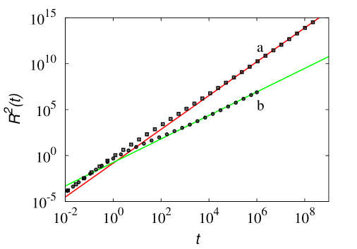
Figure 1: The mean square displacement $R^{2}(t)$ vs. time $t$ for the Wearing LW defined by eqs. (12)-(14). Dots are the results of stochastic simulations, lines represent the LW long-term scaling $R^{2}(t)\sim t^{\gamma}$. Line (a) and ($\square$) refer to $\xi=0.5$ for which $\gamma=1.84$, line (b) and ($\circ$) to $\xi=1.5$ for which $\gamma=1.28$.

Figure 1 depicts the scaling of $R^{2}(t)$ as a function of time $t$ for the WLW at the two different values of $\xi=0.5,\,1.5$. Simulations have been performed using an ensemble of $10^{7}$ particles. While for small time we observe the expected ballistic scaling, in both cases a long-term power-law scaling is observed, $R^{2}(t)\sim t^{\gamma}$, with an exponent different from the case without wearing: $\gamma=1.84\pm 0.02$ at $\xi=0.5$, whereas instead the classical LW would predict $\gamma=2$, and $\gamma=1.28\pm 0.03$ at $\xi=1.5$, with $\gamma=1.5$ instead in the absence of wearing.

A more detailed analysis of WLWs falls outside the scope of this article and will be addressed in forthcoming works. What is important to notice here is that once the age structure and formalism of LWs is assumed, generalizations and extensions of the internal age parametrization follow systematically and can be exploited for adapting the LW paradigm to the complexity of physical phenomenology.

4 Integral representation of the solutions

Here we show that the partial density formalism expressed by eqs. (3) and (5) provides the same level of analytical complexity than any other model based on the formulation of an evolution equation for the overall probability density $P(x,t)$. The approach followed is similar to a corresponding analysis developed in [35], where a single evolution equation for $P(x,t)$ was finally obtained by enforcing an initial preparation of CTRW-type. Below, starting from the hyperbolic formulation for any initial preparation, we derive a single integral equation for an auxiliary function, which depends solely on a spatial and temporal variable.

Consider the propagation of a LW on the real line, defined statistically by eqs. (3) and (5) and equipped with the initial conditions $p_{\pm}(x,0;\tau)=p^{0}_{\pm}(x,\tau)$. Assume the following initial symmetry

$$p_{+}^{0}(x,\tau)=p_{-}^{0}(-x,\tau)\quad\forall x\in{\mathbb{R}}\,,\;\tau\geq 0\quad,$$ (15)

which is the symmetry characterizing the CTRW preparation or the initial setting of a LW with aging (see Sec. 3). This symmetry involves solely the initial distribution of velocity directions and not the initial age distribution, which remains generic.

In this case, due to the symmetric propagation towards positive/negative $x$ values of the forward ($p_{+}(x,t;\tau)$) and backward ($p_{-}(x,t;\tau)$) densities, one has

$$p_{-}(x,t;\tau)=p_{+}(-x,t,\tau)\quad.$$ (16)

Consequently, in the analysis of the process it is sufficient to consider solely the forward density $p(x,t;\tau)=p_{+}(x,y;\tau)$, whose evolution equation becomes nonlocal in space according to

$$\frac{\partial p(x,t;\tau)}{\partial t} = -b\,\frac{\partial p(x,t;\tau)}{\partial x}-\frac{\partial p(x,t;\tau)}{\partial\tau}-\lambda(\tau)\,p(x,t;\tau)$$

$$p(x,t;0) = \int_{0}^{\infty}\lambda(\tau)\,p(-x,t;\tau)\,d\tau$$ (17)

$$p(x,0,\tau) = p^{0}(x,\tau)=p_{+}^{0}(x,\tau)\quad.$$

Observe that the nonlocality in eq. (17), is not a physical property but rather a mathematical superstructure introduced in order to enforce the symmetries and to get rid of the backward density wave. Obviously, the overall density $P(x,t)$ is given by

$$P(x,t)=\int_{0}^{\infty}\left[p(x,t;\tau)+p(-x,t;\tau)\right]\,d\tau\quad.$$ (18)

Consider then the transformation

$$p(x,t;\tau)=e^{-\Lambda(\tau)}\,q(x,t;\tau)\quad.$$ (19)

From eq. (17), the equation for $q(x,t;\tau)$ becomes

$$\frac{\partial q(x,t;\tau)}{\partial t}=-b\,\frac{\partial q(x,t;\tau)}{\partial x}-\frac{\partial q(x,t;\tau)}{\partial\tau}$$ (20)

equipped with the boundary and initial conditions

$$q(x,t;0) = \int_{0}^{\infty}T(\tau)\,q(-x,t,\tau)\,d\tau\quad,$$

$$q(x,0;\tau) = q^{0}(x,\tau)=e^{\Lambda(\tau)}\,p^{0}(x,\tau)\quad,$$ (21)

where $T(\tau)$ and $\Lambda(\tau)$ are defined by eq. (4). Equation (20) is a first-order constant coefficient equation casted in a conservation form that can be solved with the method of characterics: Its solution attains the form

$$q(x,t;\tau)=\phi(x-b\,t,t-\tau)\quad.$$ (22)

By considering the boundary condition at $\tau=0$, it follows that for $\tau\geq t$ $q(x,t;\tau)$ consists solely of the propagation of the initial condition both in space and age. Conversely, for $\tau<t$ the solution can be formally expressed by introducing an auxiliary function $h(x,t)$. Thus, eq. (22) can be written as

$$q(x,t;\tau)=\left\{\begin{array}[]{lll}q^{0}(x-b\,t,\tau-t)&&\tau\geq t\\ h(x-b\,\tau,t-\tau)&&\tau<t\end{array}\right.$$ (23)

Substituting eq. (23) into the boundary condition (21), the equation for $h(x,t)$ follows

$$h(x,t) = \int_{0}^{t}T(\tau)\,h(-x-b\,\tau,t-\tau)\,d\tau$$ (24)

$$+ \int_{t}^{\infty}T(\tau)\,q^{0}(-x-b\,t,\tau-t)\,d\tau\quad,$$

which holds for $t>0$. The latter equation can be obtained in terms of the initial condition $p^{0}(x,\tau)$ to

$$h(x,t) = \int_{0}^{t}T(\tau)\,h(-x-b\,\tau,t-\tau)\,d\tau$$ (25)

$$+ \int_{t}^{\infty}T(\tau)\,e^{\Lambda(\tau-t)}\,p^{0}(-x-b\,t,\tau-t)\,d\tau$$

and the density $p(x,t;\tau)$ is thus given by

$$p(x,t;\tau)=\left\{\begin{array}[]{lll}e^{-\Lambda(\tau)}\,e^{\Lambda(\tau-t)}\,p^{0}(x-b\,t,\tau-t)&&\tau\geq t\\ e^{-\Lambda(\tau)}\,h(x-b\,\tau,t-\tau)&&\tau<t\quad.\end{array}\right.$$ (26)

Since $h(x-b\,\tau,t-\tau)$ is defined stictly for $t>\tau$, it can always be set to $h(x,t)=0$ for any $x$, $t\leq 0$. Eq. (25) can be expressed equivalently as

$$h(x,t)=\int_{0}^{t}T(t-\tau)\,h(-x-b\,t+b\,\tau,\tau)\,d\tau\,,+G^{0}(t)$$ (27)

where the forcing term $G^{0}(t)$ is a linear functional of the initial condition $p^{0}(x,\tau)$ corresponding to the second integral on the r.h.s. of eq. (25). If the symmetry condition (16) is removed it is still possible to derive an integral representation of the solutions involving two auxiliary functions $h_{\pm}(x,t)$. This is addressed in Sec. 6 in connection with the analysis of the first passage time problem. Several observations follow from the above derivation:

• By applying the method of characteristics it is possible to compress all the physical information about the spatial-temporal propagation of a LW into a single function $h(x,t)$ of the two arguments $x\in{\mathbb{R}}$ and $t\geq 0$, analogously to the evolution equation associated with the overall density function $P(x,t)$ involving, for some $\lambda(\tau)$, fractional derivatives.

• Eq. (25) is exact and holds for any initial preparation of the system and any functional form of $\lambda(\tau)$.

• The memory effects of the age dynamics characterizing a LW can be clearly appreciated by the convolutional nature of the first term entering eq. (27), which is a linear Volterra integral equation whose kernel is the transition time density $T(\tau)$. Due to the simultaneous propagation both in space and along the ages, this convolution involves both arguments of the function $h(x,t)$.

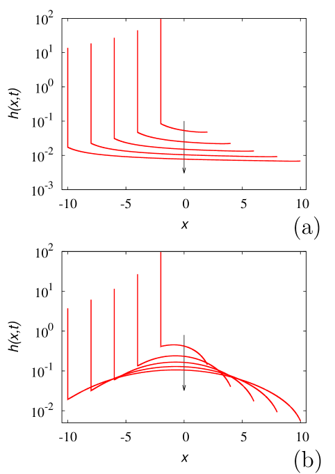
Figure 2: Function $h(x,t)$ vs. $x$ obtained from the numerical solution of the Volterra integral equation for the LW defined by the transition rate eq. (13). Panel (a) refers to $\xi=0.5$, panel (b) to $\xi=1.5$. The arrows indicate increasing time instants $t=2,\,4,\,6,\,8,\,10$.

The representation (25) is amenable to a simple numerical integration. For simplicity set $b=1$ [a.u.] and use an impulsive initial condition, $p^{0}(x,\tau)=\delta(x)\,\delta(\tau)$. For this particular case, the prefactor of $p^{0}(x-b\,t,\tau-t)$ in eq. (26) simplifies as $e^{-\Lambda(t)}$. Assuming equal step size for $x$, $t$ and $\tau$, i.e., $\Delta x=\Delta t=\Delta\tau$, and defining the grid approximation $\widehat{h}[m,n]=h(x_{m},t_{n})$, $m=\dots,-1,0,1,\dots$, $n=0,1,\dots$, where $x_{m}=m\,\Delta x$, $t_{n}=n\,\Delta t$, the simplest discretization of eq. (27) provides the solution algorithm

$$\widehat{h}[m,n]=\sum_{i=0}^{n-1}\widehat{T}[n-i]\,\widehat{h}[-m-n+i,i]\,\Delta\tau+\widehat{T}[n]\,\widehat{\delta}[m+n]\quad,$$ (28)

where $\widehat{T}[k]=T(\tau_{k})$, $\tau_{k}=k\,\Delta\tau$, and $\widehat{\delta}[h+k]$ is the numerical approximation for a Dirac delta function, $\widehat{\delta}[k]=0$ for $k\neq 0$, $\delta[0]=1/\Delta x$. For any $n$, $\widehat{h}[m,n]$ is different from zero solely for $|m|\leq n$. The overall density function $\widehat{P}[m,n]=P(x_{m},t_{n})$ at time instant $t_{n}$ is thus written as $\widehat{P}[m,n]=\widehat{\pi}[m,n]+\widehat{\pi}[-m,n]$, where

$$\widehat{\pi}[m,n]=\sum_{i=0}^{n-1}\widehat{\Lambda}[i]\,\widehat{h}[m-i,n-i]\,\Delta\tau+\widehat{\Lambda}[n]\,\widehat{\delta}[m-n]$$ (29)

and $\widehat{\Lambda}[k]=exp(-\Lambda(\tau_{k}))$. To give a numerical example, Fig. 2 depicts the evolution of the $h$-function of the LW model defined by eq. (13) at two different values of the parameter $\xi$ by applying eq. (28) with $\Delta x=10^{-3}$. The corresponding overall density profiles $P(x,t)$, derived from the $h$-function via eq. (29) and normalized to unity, are depicted in Fig. 3 by comparing them with stochastic simulations of the corresponding problem, obtained using an ensemble of $N_{p}=10^{8}$ particles. The markedly different behaviour for these two values of $\xi$ corresponds to the fact that for $\xi<1$ the LW is not transitionally ergodic i.e., no transitional age equilibrium distribution exists, while it does for $\xi>1$, where the transitional age equilibrium distribution is given by $\widehat{\pi}_{\rm equil}(\tau)=A\,e^{-\Lambda(\tau)}$ with normalization constant $A$. In the present case $\widehat{\pi}_{\rm equil}(\tau)=(\xi-1)/(1+\tau)^{\xi}$, $\xi>1$. This manifests itself in the different convexity of the distribution between the ballistic peaks, see Ref. [24] for plots of these different distributions.

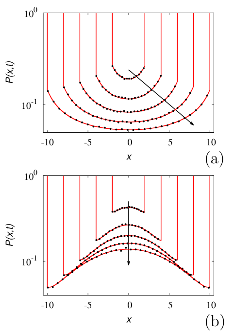
Figure 3: Overall density $P(x,t)$ vs. $x$ derived for the $h$-function depicted in Fig. 2. Panel (a) refers to $\xi=0.5$, panel (b) to $\xi=1.5$. The arrows indicate increasing time instants $t=2,\,4,\,6,\,8,\,10$. Symbols represent the results of corresponding stochastic simulations of the process.

5 Problems in bounded domains: relaxation and diffusional release dynamics

The influence of the internal preparation of a LW ensemble controls the short to intermediate scale properties and the statistical behavior in bounded systems. Let us address these issues with some examples.

5.1 Relaxational dynamics

Consider the evolution of LW fluctuations in a bounded closed domain, which in the one-dimensional case can be represented by the interval $[0,L]$. The system of hyperbolic equations (3), defined for $x\in(0,L)$, is thus equipped with reflective boundary conditions at the endpoints

$$p_{+}(0,t;\tau) = p_{-}(0,t;\tau)$$

$$p_{-}(L,t;\tau) = p_{+}(L,t;\tau)$$ (30)

for any $t>0$, $\tau>0$ corresponding to the total reflection of the incoming wave at the boundaries where it inverts its direction of propagation: at $x=0$ the incoming wave is $p_{-}(0,t;x)$, at $x=L$ it is $p_{+}(L,t;\tau)$. Independently of the transitionally ergodic nature of the age dynamics, the spatial distribution becomes asymptotically uniform, i.e., the overall density function $P(x,t)$ approaches the uniform density $P^{*}(x)=1/L$, $x\in(0,L)$ for $x\in(0,L)$ corresponding to the equilibrium distribution, at least restricted to the spatial dynamics.

Let $f(x)$ be any thermodynamic function associated with the LW fluctuations and $\overline{f}^{*}$ its equilibrium value with respect to the long-term limit density $P^{*}(x)$, i.e., $\overline{f}^{*}=\int_{0}^{L}f(x)\,P^{*}(x)\,dx$. The relaxation function $R_{f}(t)$ referred to the observable $f(x)$ is therefore the absolute value of the difference of the average value of $f(x)$ at time $t$ and its (long-term) equilibrium value $\overline{f}^{*}$,

$$R_{f}(t)=|\langle f(x)\rangle(t)-\overline{f}^{*}|=\left|\int_{0}^{L}f(x)\,P(x,t)\,dx-\frac{1}{L}\int_{0}^{L}f(x)\,dx\right|\quad.$$ (31)

The reflective conditions (30) do not alter the age structure of the LW process so that the analysis developed in the previous section, at least regarding the age dynamics, can be qualitatively applied to the present case. Suppose that the LW system is prepared in a CTRW-way with an impulsive initial age distribution $\delta(\tau)$. Consequently, during the relaxation process of the spatial distribution $P(x,t)$ towards $P^{*}(x)$, the spatial perturbation decaying in the slowest way is just the impulsive contribution associated with the sub-ensemble of fluctuations that never experienced an internal transition, which propagates back and forth at constant speed within the system due to the collisions with the endpoints and relaxing as a function of time as $e^{-\Lambda(t)}$, see eq. (26)). It follows from this observation that the relaxation function of a generic thermodynamic variable $f(x)$ for a CTRW-prepared LW ensemble should obey the long-term scaling

$$R_{f}(t)\sim e^{-\Lambda(t)}\quad.$$ (32)

Eq. (32) suggests that by modulating the functional form of the transition rates $\lambda(\tau)$ it is possible to predict from LW dynamics a great variety of relaxation phenomena observed in physical phenomenology. Specifically, consider for $\lambda(\tau)$ the model

$$\lambda(\tau)=\frac{a\,\beta}{(1+\tau)^{1-\beta}}$$ (33)

with $0<\beta<1$ and $a>0$. Since $\beta>0$, $\lim_{\tau\rightarrow\infty}\tau\,\lambda(\tau)=\infty$, $T(\tau)=a\,\beta\,(1+\tau)^{-1+\beta}\exp[1-a\,(1+\tau)^{\beta}]$, and the associated LW process is normal diffusive by possessing the whole hierarchy of moments $\langle\tau^{n}\rangle$. The Central Limit Theorem applies, and its qualitative propagation along ${\mathbb{R}}$ is, in the long-term limit, qualitatively identical to the classical mathematical Brownian motion, whose overall probability density $P(x,t)$ satisfies the parabolic diffusion equation.

Since $\Lambda(t)=a\left[(1+t)^{\beta}-1\right]$, eq. (32) indicates that the relaxational decay of any thermodynamic function $f(x)$ is of the form

$$R_{f}(t)\sim e^{-a(1+t)^{\beta}}\quad,$$ (34)

hence there is a stretched exponential decay. This decay, usually referred to as the Kohlrausch relaxation, is a common feature observed in many complex systems [58, 59]. Several interpretations have been proposed for this anomalous behavior [66, 67], but to the best of our knowledge this is the first attempt to connect it to a LW structure of the underlying fluctuations.

Equation (34) is also interesting from another thermodynamic perspective. It shows that even LW fluctuations possessing normal diffusive behavior may display highly non-trivial properties, deviating from the corresponding predictions of the associated long-term transport model. In the case of the LW process defined by eq. (33), the associated transport model, i.e., the classical hydrodynamic limit of this model, is just the parabolic diffusion equation for which the relaxation function of a generic $f(x)$ should decay exponentially as a function of time, $R_{f}(t)\sim e^{-\mu_{2}\,t}$, where $\mu_{2}>0$ is the second eigenvalue of the Laplacian operator equipped with homogeneous von Neumann conditions at the boundary. The failure of the classical hydrodynamic limit in predicting finer dynamic properties for classes of normal diffusive LWs stems from the fact that the hydrodynamic limit captures some properties of the LW dynamics, specifically the scaling of the mean square displacement, but not the entire complexity involved with a LW, which would be obtained by considering the whole moment hierarchy.

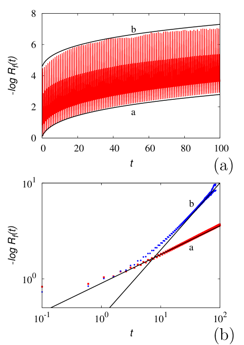
Figure 4: The relaxation function $-\log R_{f}(t)$ vs. $t$ for the relaxational dynamics in a closed system discussed in the main text using LWs defined by eq. (33) with $\beta=0.3$, $a=1$. Panel (a) shows oscillations in $R_{f}(t)$ as a function of time as explained in the text while the two curves (a) and (b) represent the envelope functions $-\log R_{f}(t)=c(1+t)^{\beta}$ for two values of the prefactor $c$. Panel (b) depicts the scaling of $-\log R_{f}(t)$ once sampled at multiples of the end-to-end transit time $L/b=1$ for $\xi=0.3$, $a=1$ (symbols ($\blacksquare$) and curve (a)), and for $\xi=0.7$, $a=0.3$ (symbols ($\bullet$) and curve (b)). Symbols are the results of stochastic simulations, lines the scaling curve derived from eq. (34), $-\log R_{f}(t)\sim(1+t)^{\beta}+c$, where $c$ is a constant.

An example of this phenomenon is depicted in Fig. 4 panel (a), where the model eq. (33) is used with $L=1$, $b=1$ [a.u.]. The relaxation data have been derived from stochastic simulations of the system using $5\times 10^{7}$ particles initially located at $x=x_{c}=1/2$ with age $\tau=0$ and equiprobable velocity directions. Statistically, this means that $p_{\pm}^{0}(x,\tau)=\delta(x-x_{c})\,\delta(\tau)/2$. As a thermodynamic test function we consider a quadratic function of $x$, $f(x)=6\,x\,(1-x)$, so that $\overline{f}^{*}=1$. Figure 4 panel (a) shows the time evolution of the logarithm of $R_{f}(t)$ with reversed sign for $\beta=0.3$, $a=1$, displaying the complex oscillations associated with the back-and-forth propagation of the impulsive mode due to the reflective boundary conditions and corresponding to the subpopulation of particles that did not experience any inner transition. The behavior of $-\log R_{f}(t)$ is highly nonlinear and bounded from below and the top by $c_{1}\,(1+t)^{\beta}<R_{f}(t)<c_{2}(1+t)^{\beta}$, where $c_{1}<c_{2}$ are constant, which is consistent with eq. (34). Taking these properties into account, if the relaxation dynamics is sampled at times $t_{n}=t_{0}+b\,L\,n$, $n=1,2,\dots$ where $t_{0}$ is any initial instant of time, a regular and monotonic behavior in the relaxation dynamics should be observed. This property is depicted in Fig. 4 panel (b) for two different LW systems.

5.2 Solute release kinetics

Significant differences controlled by the system preparation occur in other typical transport experiments involving bounded systems. Let us consider the release dynamic of a solute from a complex polymeric matrix with a transport property that obeys a LW model. Assume that $x=L$ corresponds to an impermeable boundary to solute transport and that $x=0$ is the exit boundary from which the solute is released into the environment. Moreover, assume that the external environment is perfectly mixed and arbitrarily large so that the solute concentration outside the release system, and at the exit boundary of it, can be considered vanishingly small. This transport problem is conceptually identical to a first passage time problem in which $x=0$ corresponds to the target exit point [17, 68, 69]. In the release experiment, indicating with $P_{\rm surv}(t)$ the fraction of solute particles still within the release system at time $t$ and with $J_{0}(t)$ the particle flux exiting from $x=0$, mass balance dictates

$$P_{\rm surv}(t)=1-\int_{0}^{t}J_{0}(t^{\prime})\,dt^{\prime}\quad.$$ (35)

The flux $J_{0}(t)$ in the release experiment corresponds exactly to the first passage time density function $f_{\theta_{1}}(\theta_{1})$ when $t=\theta_{1}$, i.e.,

$$f_{\theta_{1}}(\theta_{1})=-\left.\frac{dP_{\rm surv}(t)}{dt}\quad\right|_{t=\theta_{1}}.$$ (36)

Consider the LW defined by eq. (13) with $b=1$ and $L=1$. Figure 5 depicts the behavior of $P_{\rm surv}(t)$ vs. $t$ at short and intermediate time scales for the two values of $\xi=1.05,\,1.5$ corresponding to anomalous but transitionally ergodic LW fluctuations, and for two initial preparations of the system in which the solute (i.e., the LW particles) are localized initially at $x=x_{c}=1/2$ with equiprobable directions of motions and age distributions corresponding either to the CTRW preparation, i.e., $p_{\pm}(x,0,\tau)=\delta(x-x_{c})\delta(\tau)/2$, or to the equilibrium age distribution, i.e., $p_{\pm}(x,0,\tau)=\delta(x-x_{c})e^{-\Lambda(\tau)}/2$. These data have been obtained from stochastic simulations starting from an initial ensemble of $10^{8}$ solute particles.

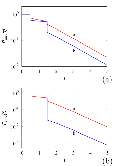
Figure 5: The survival probability density $P_{\rm surv}(t)$ vs. $t$ in a release experiment in the presence of LW particles whose motion is defined by eq. (13). Panel (a) refers to $\xi=1.5$, panel (b) to $\xi=1.05$. Lines (a) correspond to the equilibrium preparation, lines (b) to the CTRW preparation when initially all the particles possess vanishing transitional age.

One can see that the age preparation of the system deeply modifies the release properties: The difference in $P_{\rm surv}(t)$ can be of about two orders of magnitude at $\xi=1.05$ for the two preparations at time scales when a significant portion of solute is still present within the system starting from the equilibrium preparation (curve (a) in Fig. 5 panel (b)). Note also the step structure in the decay of all curves, which is due to the two propagating fronts of the particle densities and their interplay with the reflecting wall at $L$, akin to the oscillatory dynamics shown in Fig. 4. In detail, the first step corresponds to the initial solution propagating directly towards the exit point $x=0$. Conversely, the second step is generated by the initial solution propagating in the opposite direction, which is first reflected at the boundary $x=L$ and only later reaches the exit point. Recombination dynamics amongst the two partial probability waves prevents the occurrence of further jumps for longer times, and thus a smooth decaying profile sets up. While these effects, controlled by the initial conditions in age, are quantitatively relevant for transport problems, in the next section we address the peculiarity of the first passage time problem in the presence of LW fluctuations in the light of another internal parameter, namely the initial velocity direction, which plays a leading role as it emerges from the hyperbolic modelling.

6 Integral formulation of the first passage time statistics of Lévy Walks

Let us finally analyze the first passage time problem in the light of the hyperbolic formulation of the statistical properties of LWs. Owing to the analogy between LWs and Poisson-Kac processes, it is convenient to tackle this problem starting from the latter. While the main step characterizing the formulation of the hyperbolic transport equations and of the associated boundary conditions is analogous in the two cases, LWs may display some anomalies in the long-tail decay of the first passage time statistics with an exponent differing from the Sparre-Andersen value of $-3/2$ [70], which cannot occur in the classical Poisson-Kac case defined by eq. (7).

6.1 Poisson-Kac processes

Let us therefore first consider an ensemble of LW particles with $\lambda(\tau)=\lambda=\mbox{constant}$, initially localized at $x=x_{0}>0$ and evolving on the positive semiaxis, and let $x=0$ be the position of the target exit point. Once a particle passes through $x=0$ it is removed from the system, and its first passage time is evaluated. If $x(t)$ is the continuous trajectory of the particle, the first passage time $t^{*}$ is defined as the first time instant for which $x(t^{*}-\varepsilon)x(t^{*}+\varepsilon)<0$ for any small $\varepsilon>0$, provided that $x(t)>0$ for $t<t^{*}$. This case, corresponding to a Poisson-Kac ensemble, is statistically described by the hyperbolic system of equations for the partial densities $\widehat{P}_{\pm}(x,t)$ defined for $x\in(0,\infty)$ and $t>0$. At infinity regularity conditions apply, namely $\lim_{x\rightarrow\infty}x^{k}\,\widehat{P}_{\pm}(x,t)=0$ for any $t>0$ and any $k=0,1,\dots$. Regarding the condition at the exit point, the above definition of “first passage” implies the removal of any particle that passes through $x=0$ at any time $t$ from subsequent analysis. This process involves exclusively $\widehat{P}_{+}(x,t)$ at $x=0$, which should necessarily be vanishing, i.e.,

$$\widehat{P}_{+}(0,t)=0\quad.$$ (37)

Conversely, $\widehat{P}_{-}(x,t)$ can attain in principle any non-negative value at $x=0$. The exiting flux at $x=0$ is just $J_{0}(t)=b\,\widehat{P}_{-}(0,t)$ and, consequently, the first passage time density function $f_{\theta_{1}}(\theta_{1})$ is readily obtained from the solution of eqs. (7) as

$$f_{\theta_{1}}(\theta_{1})=b\,\widehat{P}_{-}(0,t)|_{t=\theta_{1}}\quad.$$ (38)

Given the initial conditions

$$\widehat{P}_{\pm}(x,0)=\pi_{\pm}^{0}\,\delta(x-x_{0})\quad,$$ (39)

$\pi_{\pm}\geq 0$, $\pi_{+}^{0}+\pi_{-}^{0}=1$, the problem expressed by eqs. (7) and equipped with the boundary condition (37), the regularity condition at infinity, and the initial condition (39) can be solved easily using Laplace transforms. The analytic expression for the first passage time statistics for PK processes has been recently discussed by Rossetto [71] starting from the Siegert formula [72]. In order to mark explicitly the dependence on the initial position $x_{0}$, it is convenient to indicate the first passage time density as $f_{\theta_{1}}(\theta_{1};x_{0})$. Although the article by Rossetto displays some typos in some basic equations, the results are correct and consequently the analysis is not repeated here. What is of relevance in the present analysis are some qualitative observations on the nature of the first passage time problem of Poisson-Kac processes. Specifically:

• This problem is intrinsically vector-valued, in the meaning that two first passage time probability densities $f_{\theta_{1}}^{(\pm)}(\theta_{1};x_{0})$ should be defined accounting for the initial preparation of the system with respect to the initial velocity orientation: $f_{\theta_{1}}^{(+)}(\theta_{1};x_{0})$ is the solution of the problem (38) for $\pi_{+}^{0}=1$, and $f_{\theta_{1}}^{(-)}(\theta_{1};x_{0})$ for $\pi_{+}^{0}=0$. Owing to linearity, the solution for generic initial conditions (39) is simply

  $$f_{\theta_{1}}(\theta_{1};x_{0})=\pi_{+}^{0}\,f_{\theta_{1}}^{(+)}(\theta_{1};x_{0})+\pi_{-}^{0}\,f_{\theta_{1}}^{(-)}(\theta_{1};x_{0})\quad.$$ (40)

  The density $f^{(-)}_{\theta_{1}}(\theta_{1};x_{0})$ admits the Laplace transform

  $${\mathcal{L}}[f^{(-)}_{\theta_{1}},s]=\exp[-(x_{0}/b)\sqrt{s}\,\sqrt{s+\lambda})]\quad,$$ (41)

  whose inverse transform is given by

  $$f_{\theta_{1}}^{(-)}(\theta_{1};x_{0}) = e^{-x_{0}\,\lambda/b}\,\delta(t-x_{0}/b)$$ (42)

  $$+ \frac{x_{0}\,\lambda}{b}\,e^{-\lambda\,t}\,\frac{I_{1}\left(\lambda\,\sqrt{t^{2}-(x_{0}/b)^{2}}\right)}{\sqrt{t^{2}-(x_{0}/b)^{2}}}\,\eta(t-x_{0}/b)\quad,$$

  where $I_{1}(\xi)$ is the modified Bessel function of the first kind of order 1 with argument $\xi$ and $\eta(\xi)$ the Heaviside step function, $\eta(y)=1$ for $y>0$, $\eta(y)=0$ for $y<0$.

• Even if initially the particles are located at $x_{0}=0$, i.e., just at the exit point, its first passage time density is not necessarily a Dirac delta $\delta(\theta_{1})$ provided that $\pi_{+}^{0}\neq 0$. Specifically it can be shown that the first passage time distribution $f_{\theta_{1}}^{(+)}(\theta_{1};0)$ is given by

  $$f_{\theta_{1}}^{(+)}(\theta_{1};0)=\lambda\,e^{-\lambda t}\,\frac{I_{1}(\lambda\,t)}{\lambda\,t}$$ (43)

  for which $f_{\theta_{1}}^{(+)}(\theta_{1};x_{0})$ follows as

  $$f_{\theta_{1}}^{(+)}(\theta_{1};x_{0})=\int_{0}^{\theta_{1}}f_{\theta_{1}}^{(-)}(\theta_{1}-\tau;x_{0})\,f^{(+)}(\tau;0)\,d\tau$$ (44)

  admitting a straightforward physical interpretation: The first passage time density from $x_{0}$ starting from an initial velocity outwardly oriented with respect the exit point (i.e., $f_{\theta_{1}}^{(+)}(\theta_{1};x_{0})$) is the convolution of the probability density of the time needed to reverse the orientation (i.e., $f^{(+)}(\tau;0)$) times the first passage time density from $x_{0}$ starting from inwardly oriented initial velocities ($f_{\theta_{1}}^{(-)}(\theta_{1}-\tau;x_{0})$).

This setting of the first passage time problem characterizes all the stochastic processes possessing finite propagation velocity including LWs.

There is another qualitative issue that distinguishes processes possessing finite propagation velocity from their Wiener-driven counterparts. This is associated with the possibility of defining the first passage time problem from an equivalent transport problem over the real line using the method of images by locating a suitable initial condition at the image point $-x_{0}$ of $x_{0}$ with respect to the exit point. Indeed, as observed in [50] this method does not apply for Lévy flights and for anomalously diffusive LWs. As a matter of fact, the method of images fails also for Poisson-Kac processes, and its failure is not related to the eventual diffusional anomaly of the process but rather to the boundedness of the propagation velocity, which is reflected in the symmetry properties of the associated Green functions for the free-space propagation.

To show this, consider the propagation of eq. (7) over the real line with an image condition at the image point $-x_{0}$,

$$\widehat{P}_{\pm}(x,0)=\pi_{\pm}^{0}\,\delta(x-x_{0})+\pi_{\pm}^{0,\prime}\,\delta(x+x_{0})\quad,$$ (45)

where $\pi_{\pm}^{0,\prime}$ are unknown real values to be determined by enforcing the boundary condition (37). The solution of this problem can be obtained by using the closed-form expression for the matrix-valued Green function reported in [62]. Indicating with $(G_{\alpha,\beta}(x,t))_{\alpha,\beta=\pm}$ the entries of the Green function matrix for an initial condition centered at $x=0$, the formal solution of the image method reads

$$\widehat{P}_{\pm}(x,t) = G_{+,+}(x-x_{0},t)\,\pi_{+}^{0}+G_{+,-}(x-x_{0},t)\,\pi_{-}^{0}$$ (46)

$$+ G_{+,+}(x+x_{0},t)\,\pi_{+}^{0,\prime}+G_{+,-}(x+x_{0},t)\,\pi_{-}^{0,\prime}\quad.$$

At $x=0$ the forwardly propagating density is

$$\widehat{P}_{+}(0,t) = \left[G_{+,+}(-x_{0},t)\,\pi_{+}^{0}+G_{+,+}(x_{0},t)\,\pi_{+}^{0,\prime}\right]$$ (47)

$$+ \left[G_{+,-}(-x_{0},t)\,\pi_{+}^{0}+G_{+,-}(x_{0},t)\,\pi_{-}^{0,\prime}\right]\quad.$$

Owing to the directed propagation of the Poisson-Kac density waves, the entries $G_{+,\pm}(x,t)$ are not symmetric functions of their spatial argument (as can be checked from their explicit analytical expression reported in [62]). Consequently, one cannot find constants $\pi_{\pm}^{0,\prime}$ such that the equations $\pi_{\pm}^{0,\prime}=-G_{+,\pm}(-x_{0},t)\,\pi_{\pm}^{0}/G_{+,\pm}(x_{0},t)$ are identically fulfilled for any $t>0$.

6.2 Lévy Walks

In the case of LWs, the first passage time problem within the hyperbolic formulation reduces to the solution of eq. (3) for the partial densities defined in $x\in(0,\infty)$ and equipped with the boundary condition for the incoming (entering) density wave

$$\left.p_{+}(0,t,\tau)\right|_{x=0}=0$$ (48)

identical to the corresponding condition (37) for Poisson-Kac processes. Indicating with $P_{\rm surv}(t)$ the fraction of particles remaining in the domain $[0,\infty)$ at time $t$, its derivative returns the probability of the first passage times with reverse sign. Enforcing the transformations

$$p_{\pm}(x,t;\tau)=e^{-\Lambda(\tau)}\,q_{\pm}(x,t;\tau)$$ (49)

the auxiliary functions $q_{\pm}(x,t;\tau)$ satisfy a conservative hyperbolic scheme

$$\frac{\partial q_{\pm}(x,t;\tau)}{\partial t}=\mp b\,\frac{\partial q_{\pm}(x,t;\tau)}{\partial x}-\frac{\partial q_{\pm}(x,t;\tau)}{\partial\tau}$$ (50)

equipped with the boundary conditions

$$q_{\pm}(x,t;0)=\int_{0}^{\infty}T(\tau)\,q_{\mp}(x,t;\tau)\,d\tau$$ (51)

and with the initial conditions $q_{\pm}(x,0;\tau)=e^{\Lambda(\tau)}\,p^{0}_{\pm}(x,\tau)=q^{0}_{\pm}(x,\tau)$.

From eq. (50) it follows that the functional dependence of the auxiliary functions on their arguments should necessarily be of the form

$$q_{\pm}(x,t;\tau)=\phi_{\pm}(x\ \mp b\,t,t-\tau)\quad.$$ (52)

To $q_{-}(x,t;\tau)$ the same representation used in Sec. 4 applies, namely

$$q_{-}(x,t;\tau)=\left\{\begin{array}[]{lll}q_{-}^{0}(x+b\,t,\tau-t)&&\tau\geq t\\ h_{-}(x+b\,\tau,t-\tau)&&\tau<t\quad.\end{array}\right.$$ (53)

Conversely, the structure of $q_{+}(x,t)$ should account for the boundary condition at $x=0$. This can be achieved by setting

$$q_{+}(x,t;\tau)=\left\{\begin{array}[]{lll}q_{+}^{0}(x-b\,t,\tau-t)&&\tau\geq t\,,\;\,x<b\,t\\ h_{+}(x-b\,\tau,t-\tau)&&\tau<t\,,\;\,\tau<x/b\\ 0&&\mbox{otherwise}\quad.\end{array}\right.$$ (54)

The latter representation ensures that no particle that left the positive region ($x>0$) will re-enter it, which is the fundamental constraint in order to define correctly the first passage time statistics.

Substituting these expressions into the boundary conditions (51), the integral equations for the auxiliary functions $h_{\pm}(x,t)$ follow. For $h_{+}(x,t)$ one derives

$$h_{+}(x,t) = \int_{0}^{t}T(t-\tau)\,h_{-}(x+b\,t-b\,\tau,\tau)\,d\tau$$ (55)

$$+ \int_{t}^{\infty}T(\tau)\,e^{\Lambda(\tau-t)}\,p_{-}^{0}(x+b\,\tau,\tau-t)\,d\tau\quad.$$

For $h_{-}(x,t)$ eq. (54) provides

$$h_{-}(x,t) = \int_{0}^{t}T(\tau)\,h_{+}(x-b\,\tau,t-\tau)\,\eta(x-b\,\tau)\,d\tau$$ (56)

$$+ \,\eta(x-b\,t)\int_{t}^{\infty}T(\tau)\,e^{\Lambda(\tau-t)}\,p_{+}^{0}(x-b\,t,\tau-t)\,d\tau\quad,$$

where $\eta(\cdot)$ is the Heaviside step function. Alternatively, the first integral on the r.h.s of eq. (56) can be expressed as

$$\int_{0}^{\mbox{min}\{t,x/b\}}T(\tau)\,h_{+}(x-b\,\tau,t-\tau)\,d\tau\quad.$$

The quantity $1-P_{\rm surv}(t)$ represents the distribution function for the first passage times and the corresponding density follows from differentiation, see eq. (36). $P_{\rm surv}(t)$ can be readily obtained from the solution of the above integral equations, since by definition $P_{\rm surv}(t)=\int_{0}^{\infty}dx\int_{0}^{\infty}\left[p_{+}(x,t;\tau)+p_{-}(x,t;\tau)\right]\,d\tau$.

The system of eqs. (55)-(56) has been solved numerically for a LW with $b=1$ [a.u.] with the transition rate function expressed by eq. (13) using $\Delta x=\Delta t=\Delta\tau=10^{-2}$. As an initial preparation, consider the case $p_{\pm}(x,\tau)=\pi_{\pm}^{0}\,\delta(x-x_{0})\,\delta(\tau)$, with $x_{0}=1$, and different settings of the probabilistic weights $\pi_{\pm}^{0}>0$, $\pi_{+}^{0}+\pi_{-}^{0}=1$, controlling the distribution of the initial velocity directions. Figure 6 depicts the behaviour of $P_{\rm surv}(t)$ vs. $t$ obtained from the numerical solution of the integral Volterra equations for $\xi=0.5$ and different initial velocity direction distributions, compared with the corresponding data obtained from the stochastic simulations of the first passage time problem using an ensemble of $10^{8}$ particles.

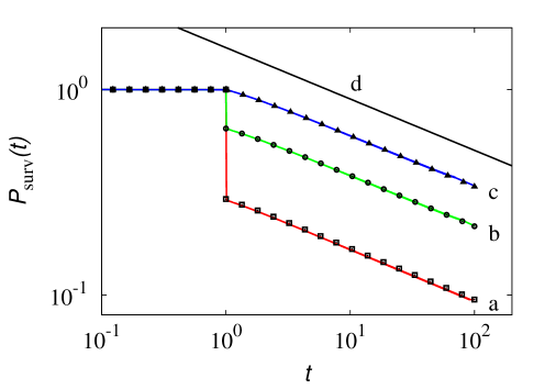
Figure 6: The survival probability $P_{\rm surv}(t)$ vs. $t$ for the LW defined by eq. (13), $\xi=0.5$, with $b=1$, $x_{0}=1$, for different values of $\pi_{+}^{0}$. Solid lines (a)-(c) are the results of the numerical integration of eqs. (55)-(56) with $\Delta t=10^{-2}$, symbols the results of stochastic simulations. Line (a) and ($\square$) refers to $\pi_{+}^{0}=0$, line (b) and ($\circ$) to $\pi_{+}^{0}=0.5$, line (c) and ($\triangle$) to $\pi_{+}^{0}=1$. The solid line (d) represents the scaling $P_{\rm surv}(t)\sim t^{-\xi/2}$.

Scaling theory provides for the first passage time density $f_{\theta_{1}}(\theta_{1})\sim\theta_{1}^{-\zeta}$, $\theta_{1}\gg x_{0}/b$. For $\xi>1$ we obtain the exponent $\zeta=3/2$ corresponding to the Sparre-Andersen result while for $\xi<1$ we get $\zeta=1+\xi/2$ [73, 74]. In terms of the survival fraction $P_{\rm surv}(t)$ this means

$$P_{\rm surv}(t)\sim\left\{\begin{array}[]{lll}t^{-\xi/2}&&0<\xi<1\\ t^{-1/2}&&\xi>1\quad.\end{array}\right.$$ (57)

The integration of the system of equations for $h_{\pm}(x,t)$ closely matches the stochastic data and correctly predicts the anomalous Sparre-Andersen exponent.

However, one should be cautious with the numerical integration of eqs. (55)-(56), as the accuracy may depend significantly on the step size chosen. This phenomenon is depicted in Fig. 7 at $\xi=1.5$ in which a step size of at least $\Delta t=10^{-3}$ is required for an acceptable prediction of the stochastic simulation data. This opens up the interesting problem of defining novel numerical algorithms for the efficient integration of the integral Volterra equations arising from LW theory, a problem that is shared by any model expressed in terms of the fractional derivatives of the overall distribution function $P(x,t)$.

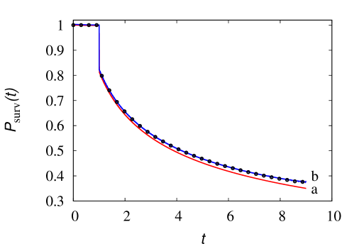
Figure 7: $P_{\rm surv}(t)$ vs. $t$ for the LW defined by eq. (13), $\xi=1.5$, with with $b=1$, $x_{0}=1$ and $\pi_{0}^{+}=0.5$. Solid lines represent the result of the numerical integration of eqs. (55)-(56) at two different step sizes: (a) $\Delta t=10^{-2}$, (b) $\Delta t=10^{-3}$. Symbols are the results of stochastic simulations.

7 Concluding remarks

The hyperbolic formulation of LWs, parametrized with respect to the velocity direction and the transitional age, permits to completely describe their statistical properties in a simple formal setting, which makes it possible to address a variety of different phenomenologies within a unified framework. The concept of ensemble preparation is a direct consequence of this formulation accounting for the more general case of initial conditions involving the internal degrees of freedom characterizing LWs. In this framework, the concept of aging emerges as a particular system preparation.

However, to conceptually simple theoretical settings do not necessarily correspond computationally simple ways of determining the respective system properties. Nevertheless, in the case of the hyperbolic formulation of the statistical properties of LWs, the extra degree of freedom represented by the transitional age $\tau$, which comes in addition to the two variables of space coordinate $x$ and time $t$ in the partial densities $p_{\pm}(x,t;\tau)$, can be embedded within the temporal parametrization. This means that the evolution of the system can be completely described by means of two auxiliary function $h_{\pm}(x,t)$ depending exclusively on a space $x$ and a temporal coordinate $t$, satisfying a system of Volterra integral equations in which the convolutional nature of the dynamics accounts for the memory effects associated with the age. In general, as for Poisson-Kac processes the parametrization with respect to the velocity direction, which corresponds to the inclusion of a system of two partial densities $p_{\pm}(x,t;\tau)$ (or two auxiliary functions $h_{\pm}(x,t)$) in the statistical analysis cannot be eliminated if the most general initial preparations are considered in which unbalanced subpopulations of particles initially moving in the two opposite directions may occur.

If symmetric conditions for the initial population of the forward and backward moving particles are assumed, only a single auxiliary function, say $h(x,t)=h_{+}(x,t)$ is needed in the free-space propagation, as for any model involving the overall density function $P(x,t)$, allowing an arbitrary initial age preparation of the system. The equation for $h(x,t)$ becomes nonlocal, and the nonlocality reflects the reduction of the model to a single propagating field. This presents some similarities with the problem of nonlocality and hidden variables in quantum mechanics, where the notion of hidden variables is not solely related to the existence of a “hidden probabilitistic structure” [75] but eventually to the inclusion of neglected propagating fields [76].

The importance of correctly accounting for the initial preparation of the system emerges clearly either in the short/intermediate term dynamics or in problems defined in bounded domains. Even diffusionally regular LWs displaying a linear scaling in the mean square displacement may show interesting anomalous relaxation properties, such as the occurrence of a stretched exponential decay. This example suggests a broader application of LW fluctuations in material science and polymer physics as a model of complex fluctuations (viscoelasticity, nonlinear viscoelasticity, etc.).

The analysis of the first passage time statistics embedded within the hyperbolic formalism opens up several interesting pathways for further investigation. The difficulty with formulating a correct method of images for the first passage time problem involving LWs is not related to their anomalous behavior but is intrinsically rooted in the finite propagation velocity of these fluctuation models. The mathematical setting of this problem in terms of partial densities requires that the partial density associated with an incoming wave from the surrounding environment should vanish at the target exit boundary in order not to reinject particles into the domain that have already been passed through it. The same problem arises in other classes of dynamics possessing finite propagation velocity such as Poisson-Kac processes. The manipulation of the partial density equations, enforcing the method of characteristics, permits to reduce the transport problem to the evaluation of two auxiliary functions $h_{\pm}(x,t)$ of the spatial coordinate $x$ and the temporal one $t$, as in the case of the free-space propagation.

The hyperbolic formulation of LWs is particularly suited for modelling more complex situations, which account for the occurrence of interparticle interactions, exclusion effects, etc., that in a mean-field modeling can be described by allowing the velocity $b$ and the transition rate $\lambda(\tau)$ to depend on the partial wave densities. This extension has been initiated in [77, 78] for LWs and in [79] for Poisson-Kac processes.

Acknowledgements: R.K. thanks Professors Klapp and Stark (TU Berlin) for hospitality. He is also grateful for funding from the Office of Naval Research Global and from the London Mathematical Laboratory, where he is an External Fellow. A.C. gratefully acknowledges funding under the Science Research Fellowship granted by the Royal Commission for the Exhibition of 1851. M.G., A.C. and R.K. thank the London Mathematical Laboratory for hospitality during and after a workshop, where this article was completed.

References

References

- [1] Chandrasekhar S 1943 Stochastic problems in physics and astronomy Rev. Mod. Phys. 15 1
- [2] van Kampen N 1992 Stochastic Processes in Physics and Chemistry (Amsterdam: North Holland)
- [3] Kleinert H 1989 Gauge Fields in Condensed Matter. Vol II: Stresses and Defects (Singapore: World Scientific)
- [4] Weiss G H (1994) Aspects and Applications of the Random Walk (Amsterdam: North-Holland)
- [5] Kipnis C and Landim C 1999 Scaling Limits of Interacting Particle Systems (Berlin: Springer-Verlag)
- [6] De Masi A and Presutti E 1991 Mathematical Methods for Hydrodynamic Limits (Berlin: Springer-Verlag)
- [7] Giona M 2018 Lattice random walk: an old problem with a future ahead Phys. Scripta 93 095201
- [8] Spitzer F 1970 Interaction of Markov processes Adv. Math. 5 246
- [9] Krapivsky P L, Redner S and Ben-Naim E 2010 A Kinetic View of Statistical Physics (Cambridge: Cambridge University Press)
- [10] Solon A P and Tailleur J 2013 Revisiting the flocking transition using active spins Phys. Rev. Lett. 111 078101
- [11] Solon A P and Tailleur J 2015 Flocking with discrete symmetry: The two-dimensional active Ising model Phys. Rev. E 92 042119
- [12] Coopersmith M and Mandeville G 1974 Irreversible behavior of interacting systems. I. The approach to equilibrium J. Stat. Phys. 10 391
- [13] Gottwald G A and Oliver M 2009 Boltzmann’s Dilemma: An Introduction to Statistical Mechanics via the Kac Ring SIAM Rev. 51 613
- [14] Montroll E W and Weiss G H 1965 Random walks on lattices. II J. Math. Phys. 6 167
- [15] Kenkre V M, Montroll E W and Shlesinger M F 1973 Generalized master equations for continuous-time random walks J. Stat. Phys. 9 45
- [16] Klafter J and Silbey R 1980 Derivation of the continuous-time random-walk equation Phys. Rev. Lett. 44 55
- [17] Hughes B D 1995 Random Walks and Random Environments (Oxford: Clarendon Press).
- [18] Metzler R and Klafter J 2000 The random walk’s guide to anomalous diffusion: a fractional dynamics approach Phys. Rep. 339
- [19] Metzler R and Klafter J 2004 The restaurant at the end of the random walk: recent developments in the description of anomalous transport by fractional dynamics J. Phys. A 37 R161
- [20] Klages R, Radons G and Sokolov I M (Editors) 2008 Anomalous transport: Foundations and Applications (Berlin: Wiley-VCH)
- [21] Shlesinger M F, Klafter J and Wong Y 1982 Random walks with infinite spatial and temporal moments J. Stat. Phys. 27 499
- [22] Shlesinger M F, West B J and Klafter J 1987 Lévy dynamics of enhanced diffusion: Application to turbulence Phys. Rev. Lett. 58 1100
- [23] Klafter J, Blumen A and Shlesinger M F 1987 Stochastic pathway to anomalous diffusion Phys. Rev. E 35 3081
- [24] Zaburdaev V, Denisov S, Klafter J 2015 Lévy walks Rev. Mod. Phys. 87 483
- [25] Magdziarz M and Zorawik T 2016 Densities of scaling limits of coupled continuous time random walks Fract Calc Appl Anal 19 1488-1506
- [26] Zumofen G and Klafter J 1993 Scale-invariant motion in intermittent chaotic systems Phys. Rev. E 47 851
- [27] Stefani F D, Hoogenboom J P and Barkai E 2009 Beyond quantum jumps: blinking nanoscale light emitters Phys. Tod. 62 34
- [28] Ariel G, Rabani A, Benisty S, Partridge J D, Harshey R M and Be’er A 2015 Swarming bacteria migrate by Lévy Walk Nature Comm. 6 8396
- [29] Harris T H et al. 2012 Generalized Lévy walks and the role of chemokines in migration of effector CD8+ T cells Nature 486 545
- [30] Viswanathan G M, da Luz M G E, Raposo E P and Stanley H E 2011 The Physics of Foraging (Cambridge: Cambridge University Press)
- [31] Sokolov I M and Metzler R 2003 Towards deterministic equations for Lévy walks: The fractional material derivative Phys. Rev. E 67 010101(R)
- [32] Magdiarz M, Szczotka W and Zebrowski P 2012 Langevin picture of Lévy walks and their extensions J Stat. Phys. 147 74
- [33] Taylor-King J P, Klages R, Fedotov S and Van Gorder R A 2016 Fractional diffusion equation for an -dimensional correlated Lévy walk Phys. Rev. E 94 012104
- [34] Zaburdaev V, Fouxon I, Denison S and Barkai E 2016 Superdiffusive dispersals impart the geometry of underlying random walks Phys. Rev. Lett. 117 270601
- [35] Fedotov S 2016 Single integrodifferential wave equation for a Lévy walk Phys. Rev. E 93, 020101(R)
- [36] Fedotov S, Tan A and Zubarev A 2015 Persistent random walk of cells involving anomalous effects and random death Phys. Rev. E 91 042124
- [37] Shkilev V P 2017 Continuous-time random walk under time-dependent resetting Phys. Rev. E 96 012126
- [38] Shkilev V P 2018 Subordinated stochastic processes with aged operational time Phys. Rev. E 97 012102
- [39] Goldstein S 1951 On diffusion by discontinuous movements, and on the telegraph equation Quart. J. Mech. Appl. Math. 4 129
- [40] Kac M 1956 Some Stochastic Problems in Physics and Mathematics (Socony Mobil Oil Company Colloquium Lectures, USA)
- [41] Kac M 1974 A stochastic model related to the telegrapher’s equation Rocky Mount. J. Math. 4 497
- [42] Weiss G H 2002 Some applications of persistent random walks and the telegrapher’s equation Physica A 311 381
- [43] Bena I 2006 Dichotomous Markov noise: exact results for out-of-equilibrium systems Int. J. Mod. Phys. B 20 2825
- [44] Giona M, Brasiello A and Crescitelli S 2017 Stochastic foundations of undulatory transport phenomena: generalized Poisson–Kac processes–part I basic theory J. Phys A 50 335002
- [45] Giona M, Brasiello A and Crescitelli S 2017 Stochastic foundations of undulatory transport phenomena: generalized Poisson–Kac processes–part II Irreversibility, norms and entropies J. Phys A 50 335003
- [46] Giona M, Brasiello A and Crescitelli S 2017 Stochastic foundations of undulatory transport phenomena: generalized Poisson–Kac processes–part III extensions and applications to kinetic theory and transport J. Phys A 50 335004
- [47] Dhar A, Kundu A, Majumdar S N, Sabhapandit S and Schehr G 2019 Run-and-tumble particle in one-dimensional confining potentials: Steady-state, relaxation, and first-passage properties Phys Rev E 99 032132
- [48] Malakar K, Jemseena V, Kundu A, Vijay Kumar K, Sabhapandit S, Majumdar S N, Redner S and Dhar A 2018 Steady state, relaxation and first-passage properties of a run-and-tumble particle in one-dimension J Stat Mech 043215.
- [49] Magdiarz M and Zorawik T 2015 Densities of Lévy walks and the corresponding fractional equations arXiv:1504.05835
- [50] Chechkin A V, Metzler R, Gonchar, Klafter J and Tanatarov L V 2003 First passage and arrival time densities for Lévy flights and the failure of the method of images J. Phys. A 36 L537
- [51] Barkai E 2003 Aging in subdiffusion generated by a deterministic dynamical system Phys. Rev. Lett. 90 104101
- [52] Barkai E and Cheng Y-C 2003 Aging continuous time random walks J. Chem. Phys. 118 6167
- [53] Magdziarz M and Zorawik T 2017 Aging ballistic Lévy walks Phys. Rev. E 95 022126
- [54] Froemberg D and Barkai E 2013 Time-averaged Einstein relation and fluctuating diffusivities for the Lévy walk Phys. Rev. E 87 030104
- [55] Metzler R, Jeon J-H, Cherstvy A G and Barkai E 2014 Anomalous diffusion models and their properties: non-stationarity, non-ergodicity, and ageing at the centenary of single particle tracking Phys. Chem. Chem. Phys. 16 24128 kkk
- [56] Albers T and Radons G 2018 Exact results for the nonergodicity of d-dimensional generalized Lévy walks Phys. Rev. Lett. 120 104501
- [57] Bothe M, Sagues F and Sokolov I M 2019 Mean squared displacement in a generalized Lévy walk model, preprint arXiv1903.09505
- [58] Williams G and Watts D C 1970 Non-symmetrical dielectric relaxation behaviour arising from a simple empirical decay function Trans. Faraday Soc. 66 80
- [59] Phillips J C 1996 Stretched exponential relaxation in molecular and electronic glasses Rep. Prog. Phys. 59 1133
- [60] Wong E and Zakai M 1965 On the relation between ordinary and stochastic differential equations Int. J. Eng. Sci. 3 213
- [61] Wong E, Zakai M 1965 On the convergence of ordinary integrals to stochastic integrals Ann. Math. Stat. 36 1560
- [62] Giona M and Pucci L 2019 Hyperbolic heat/mass transport and stochastic modelling–Three simple problems Mathematics in Engineering 1 224
- [63] Criado-Sancho M and Llebot J E 1993 On the admissible values of the heat flux in hyperbolic heat transport Phys. Lett. A 177 323
- [64] Camacho J 1995 Third law of thermodynamics and maximum heat flux Phys. Lett. A 202 88
- [65] Brasiello A, Crescitelli S and Giona M 2016 One-dimensional hyperbolic transport: Positivity and admissible boundary conditions derived from the wave formulation Physica A 449 176
- [66] Shlesinger M F and Klafter J 1986 On the relationship among three theories of relaxation in disordered systems Proc. Natl. Acad. Sci. USA 83 848
- [67] Magdiarz M and Weron K 2006 Anomalous diffusion schemes underlying the stretched exponential relaxation. The role of subordinators Acta Phys. Pol. B 37 1617
- [68] Redner S 2001 A Guide to First Passage Processes (Cambridge: Cambridge University press)
- [69] Metzler R, Oshanin G and Redner S (Editors) 2014 First-Passage Phenomena and Their Applications (Singapore: World Scientific)
- [70] Dybiec E, Gudowska-Nowak E, Barkai E and Dubkov A A 2017 Lévy flights versus Lévy walks in bounded domains Phys Rev E 95 052102
- [71] Rossetto V 2018 The one-dimensional asymmetric persistent random walk J. Stat. Mech. 043204
- [72] Siegert A J F 1951 On the first passage time probability problem Phys. Rev. 81 617
- [73] Korabel N and Barkai E 2011 Anomalous infiltration J. Stat. Mech. P05022
- [74] Artuso R, Cristadoro G, Esposti M D and Knight G 2014 Sparre-Andersen theorem with spatiotemporal correlations Phys Rev E 89, 052111
- [75] Wheeler J A, Zurek W H 1983 Quantum Theory and Measurement (Princeton: Princeton University Press)
- [76] Rashkovskiy SA 2017 What does a violation of the Bell’s inequality prove? arXiv:1701.03700
- [77] Fedotov A, Korabel N 2017 Emergence of Lévy walks in systems of interacting individuals Phys. Rev. E 95 030107
- [78] Stage H, Fedotov S 2017 Non-linear continuous time random walk models Eur. Phys. J. B 90 225
- [79] Giona M 2018 Generalized Poisson-Kac processes and hydrodynamic modeling of systems of interacting particles I – Theory arXiv: 1806.03266