Nonlinear thermoelectricity with electron-hole symmetric systems

Abstract

In the linear regime, thermo-electric effects between two conductors are possible only in the presence of an explicit breaking of the electron-hole symmetry. We consider a tunnel junction between two electrodes and show that this condition is no longer required outside the linear regime. In particular, we demonstrate that a thermally-biased junction can display an absolute negative conductance (ANC), and hence thermo-electric power, at a small but finite voltage bias, provided that the density of states of one of the electrodes is gapped and the other is monotonically decreasing. We consider a prototype system that fulfills these requirements, namely a tunnel junction between two different superconductors where the Josephson contribution is suppressed. We discuss this nonlinear thermo-electric effect based on the spontaneous breaking of electron-hole symmetry in the system, characterize its main figures of merit and discuss some possible applications.

Introduction. Recently, thermal transport at the nanoscale and the field of quantum thermodynamics have attracted a growing interest Benenti et al. (2017); Dubi and Di Ventra (2011); Kosloff (2013); Seifert (2012); Muhonen et al. (2012); Campisi et al. (2011); Giazotto et al. (2006); Fornieri and Giazotto (2017); Brunner et al. (2012); Barato and Seifert (2015); Polettini et al. (2015); Verley et al. (2014); Pietzonka and Seifert (2018); Manikandan et al. (2019). In particular, thermo-electric systems have been extensively investigated Claughton and Lambert (1996); Brandner et al. (2013); Sothmann et al. (2014); Ozaeta et al. (2014); Esposito et al. (2009); Vischi et al. (2019); Whitney (2014); Giazotto et al. (2015); Ronetti et al. (2016); Giazotto et al. (2014); Marchegiani et al. (2016); Kamp and Sothmann (2019), since they provide a direct thermal-to-electrical power conversion. In a two-terminal system, a necessary condition for thermoelectricity in the linear regime, i.e., for a small voltage $V$ and a small temperature bias $\Delta T$, is breaking the electron-hole (EH) symmetry which results in the transport property $I(V,\Delta T)\neq-I(-V,\Delta T)$, where $I$ is the charge current flowing through the two-terminal system. In fact, if $I(V,\Delta T)=-I(-V,\Delta T)$, it follows $I(0,\Delta T)=0$, and hence a null thermopower, irrespectively of the temperature bias $\Delta T$. Nonlinear thermoelectric effects have been also investigated Azema et al. (2014); Kim et al. (2014); Zimbovskaya (2015); Svilans et al. (2016); Sánchez and Serra (2011); Boese and Fazio (2001); Sánchez and López (2016); Whitney (2013); Erdman et al. (2019), even in systems where $I(0,\Delta T)=0$ Hwang et al. (2015), but the EH symmetry breaking is always assumed. For metals, the EH symmetry is roughly present for Landau-Fermi liquids at small energies, and indeed thermoelectric effects in real metals are typically small, scaling as $T/T_{\rm F}$, where $T_{\rm F}$ is the Fermi temperature. More generally, a nearly perfect EH symmetry characterizes many interacting systems in the quantum regime, such as superconductors Tinkham (2004); de Gennes (1999) or Dirac materials Wehling et al. (2014).

Here, we establish a set of sufficient and universal conditions for finite thermoelectric power $\dot{W}=-IV>0$ in systems where EH symmetry holds $I(V,\Delta T)=-I(-V,\Delta T)$. More precisely, we demonstrate that the electron-hole symmetry breaking which leads to thermoelectricity is driven by the nonlinear temperature difference and asymmetry between the two terminals.

Model. We consider a basic example in quantum transport, namely a tunnel junction, which is also experimentally relevant. The system consists of two conducting electrodes (L, R), coupled through a thin insulating barrier, where quantum tunnelling takes place. In this case, the main contribution to transport is typically given by Landau’s fermionic excitations, called quasiparticles. For the purpose of our discussion, we assume each electrode in internal thermal equilibrium, namely the quasiparticle distributions read $f_{\alpha}(E-\mu_{\alpha})=\{1+\exp[(E-\mu_{\alpha})/(k_{\rm B}T_{\alpha})]\}^{-1}$, where $k_{\rm B}$ is the Boltzmann constant and $T_{\alpha}$, $\mu_{\alpha}$ (with $\alpha=$L, R) are the temperatures and the chemical potentials of the quasiparticle systems, respectively. The quasiparticle charge and heat current flowing out of the $\alpha$-electrode (with $\bar{\alpha}={\rm R}$ when $\alpha={\rm L}$ and vice versa) read Mahan (2000); Tinkham (2004)

$$\begin{pmatrix}I_{\alpha}\\ \dot{Q}_{\alpha}\end{pmatrix}=\frac{G_{\rm T}}{e^{2}}\int_{-\infty}^{+\infty}dE\begin{pmatrix}-e\\ E_{\alpha}\end{pmatrix}N_{\alpha}(E_{\alpha})N_{\bar{\alpha}}(E_{\bar{\alpha}})F_{\alpha}(E_{\alpha})$$ (1)

where $-e$ is the electron charge, $N_{\alpha}(E)$ is the quasiparticle density of states (DoS), $F_{\alpha}(E_{\alpha})=f_{\alpha}(E_{\alpha})-f_{\bar{\alpha}}(E_{\bar{\alpha}})$, $E_{\alpha}=E-\mu_{\alpha}$, and $G_{\rm T}$ is the conductance of the junction if both the electrodes have constant $N_{\alpha}$. For simplicity, we assumed spin-degeneracy, and an energy and spin independent tunneling in the derivation of Eq. 1. We consider EH symmetric DoSs: $N_{\alpha}(E)=N_{\alpha}(-E)$ and we define $I=I_{\rm L}$ . Under a voltage bias $V\neq 0$, the chemical potentials are shifted: $\mu_{\rm L}-\mu_{\rm R}=-eV$. By exploiting the symmetries, one can show that $I(V,T_{\rm L},T_{\rm R})=-I(-V,T_{\rm L},T_{\rm R})$ and $\dot{Q}_{\alpha}(V,T_{\rm L},T_{\rm R})=\dot{Q}_{\alpha}(-V,T_{\rm L},T_{\rm R})$ SM . The expressions of Eq. 1 respect the thermodynamic laws Benenti et al. (2017); Whitney (2013); Prigogine (1955); de Groot and Mazur (1962). In particular, the energy conservation in the junction reads $\dot{Q}_{\rm L}+\dot{Q}_{\rm R}+IV=0$ (first law), and the entropy production rate $\dot{S}=-\dot{Q}_{\rm L}/T_{\rm L}-\dot{Q}_{\rm R}/T_{\rm R}$ is not negative (second law) Benenti et al. (2017); Yamamoto and Hatano (2015); Whitney (2013). As a consequence, for $T_{\rm L}=T_{\rm R}=T$ it follows $IV\geq 0$. Conversely, for $T_{\rm L}\neq T_{\rm R}$, the condition $IV<0$ is possible. For instance, in a thermo-electric generator, the condition $\dot{W}=-IV>0$ is thermodynamically consistent with the constraint $\dot{S}\geq 0$ if the efficiency of the conversion $\eta=\dot{W}/\dot{Q}_{\rm hot}$ is not larger than the Carnot efficiency, $\eta\leq\eta_{\rm C}=1-T_{\rm cold}/T_{\rm hot}$ ($\dot{Q}_{\rm hot}>0$ is the heat current from the hot lead).

Consider the charge current $I$ from Eq. 1. Essentially, the condition on the existence of a thermo-electric power $\dot{W}>0$ can be expressed as the possibility of having an absolute negative conductance (ANC), $I(V)/V<0$, under a thermal bias. Thanks to EH symmetry, we can focus on $V>0$ and ask whether we can have $I(V,T_{\rm L},T_{\rm R})<0$ for $T_{\rm L}\neq T_{\rm R}$. With no loss of generality, we assume here and in the rest of this work $T_{\rm L}\geq T_{\rm R}$, with $\Delta T=T_{\rm L}-T_{\rm R}$. For $N_{\rm L}(E)=N_{\rm R}(E)$, one can prove that $I(V)\geq 0$ for $V>0$, namely two different DoSs are necessary for thermoelectricity in the presence of EH symmetry SM . Our goal is to derive sufficient conditions on the two DoSs which guarantee the existence of thermoelectricity.

To this end, it is convenient to measure the energy $E$ with respect to $\mu_{\rm L}$, i.e., we set $\mu_{\rm L}=0$, $\mu_{\rm R}=eV$. We rewrite, with simple manipulations, the charge current $I$ of Eq. 1 as

$$I=\frac{G_{\rm T}}{e}\int_{0}^{\infty}dEN_{\rm L}(E)f_{\rm L}(E)[N_{\rm R}(E_{+})-N_{\rm R}(E_{-})]+$$

$$\frac{G_{\rm T}}{e}\int_{0}^{\infty}dEN_{\rm L}(E)[N_{\rm R}(E_{-})f_{\rm R}(E_{-})-N_{\rm R}(E_{+})f_{\rm R}(E_{+})]$$ (2)

where $E_{\pm}=E\pm eV$. If $N_{\rm L}$ is a gapped function (with gap $\Delta_{\rm L}$), that is $N_{\rm L}\approx 0$ for $|E|<\Delta_{\rm L}$, the second term in Eq. 2 is negligible when $eV,k_{\rm B}T_{\rm R}\ll\Delta_{\rm L}$, due to the exponential damping of the cold distribution $f_{\rm R}$ above the gap $\Delta_{\rm L}$. Moreover, for $k_{\rm B}T_{\rm L}\sim\Delta_{\rm L}$, the integrand function in the first term of Eq. 2 is finite, owing to the presence of the hot distribution $f_{\rm L}$, and negative when $N_{\rm R}(E)$ is a monotonically decreasing function for $E>\Delta_{\rm L}-eV$. In conclusion, even with EH symmetric DoSs, the presence of a gap in the hot electrode DoS and the monotonically decreasing function in the cold electrode DoS may generate an ANC, and hence thermoelectricity $\dot{W}=-IV>0$. This is the crucial result of this work, and can be applied in a quite general setting SM . Below, we discuss the main features of this nonlinear thermoelectric effect for an experimentally suitable EH symmetric system: a tunnel junction between two Bardeen-Cooper-Schrieffer (BCS Bardeen et al. (1957)) superconductors (SIS junction).

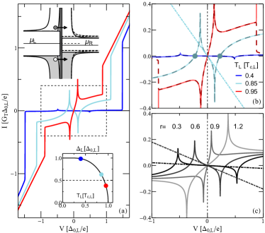
Figure 1: (color online). (a) Quasiparticle current-voltage characteristic of a thermally biased tunnel junction between two superconductors (SIS junction) for $T_{\rm R}=0.01T_{\rm c,L}$, $r=0.5$ and different values of $T_{\rm L}>T_{\rm R}$. The curves display absolute negative conductance (ANC) and thermoelectric power $\dot{W}=-IV>0$ at small voltage bias if $\Delta_{\rm L}(T_{\rm L})>\Delta_{\rm 0,R}$. Top inset: energy band diagram of the SIS junction. The combination of the gap in the hot electrode (left) and the monotonically decreasing DoS above gap of the cold electrode (right) produces a particle current which flows in the opposite direction of the chemical potential gradient. Bottom inset: temperature dependence of the superconducting gap $\Delta_{\rm L}$. Colored points mark the values of $\Delta_{\rm L}(T_{\rm L})$ for the curves displayed in the panel a). The horizontal dashed line intercepts the $\Delta_{\rm L}$ curve at the point where $\Delta_{\rm L}(T_{\rm L})=\Delta_{\rm 0,R}$, i.e., the maximum temperature for the existence of the ANC in panels (a) and (b). b) Enlargement of the subgap transport in panel (a) (dashed rectangle). Dashed curves give the first term of Eq. 2. The light-blue dots give the values of the Seebeck voltage $V_{\rm S}$. (c) Subgap IV characteristics for $T_{\rm L}=0.7T_{\rm c,L}$, $T_{\rm R}=0.01T_{\rm c,L}$, and different values of $r$. The slopes of the dash-dotted lines in panels (b) and (c) give the values of the ANC at $V\approx 0$, as expressed by Eq. 3.

SIS junction. For simplicity, we focus on quasiparticle transport and assume to completely suppress the Josephson contribution occurring in SIS junctions Fornieri and Giazotto (2017); Pershoguba and Glazman (2019); Guarcello et al. (2019). This condition can be achieved either by considering a junction with a strongly oxidized barrier or by appropiately applying an external in-plane magnetic field. The quasiparticle DoS reads $N_{\alpha}=\theta(|E|-\Delta_{\alpha})|E|/\sqrt{E^{2}-\Delta_{\alpha}^{2}}$ , where $\Delta_{\rm\alpha}(T_{\alpha})$ are the temperature dependent superconducting order parameters. In particular, $\Delta_{\rm\alpha}(T_{\rm\alpha}=0)=\Delta_{\rm 0,\alpha}$ and it decreases monotonically with $T_{\rm\alpha}$, following a universal relation, obtained through a self-consistent calculation Tinkham (2004) (see the bottom inset of Fig.1a). It becomes zero when the temperature approaches the critical value $T_{\rm c,\alpha}=\Delta_{\rm 0,\alpha}/(1.764k_{\rm B})$. We stress that the temperature dependence of $\Delta_{\rm\alpha}$ is not necessary for the mechanism, and it is characteristic of the specific system here considered.

Since $N_{\rm L}(E)\neq N_{\rm R}(E)$ is a necessary condition for thermoelectricity, hereafter we consider the case where the two gaps at zero-temperature differ introducing a parameter $r=\Delta_{\rm 0,R}/\Delta_{\rm 0,L}=T_{\rm c,R}/T_{\rm c,L}$.

Consider now Eq. 2 for a SIS junction. As discussed above, for $eV,k_{\rm B}T_{\rm R}\ll\Delta_{\rm L}(T_{\rm L})$ the second term is negligible and $I(V)$ is given entirely by the first contribution. To have ANC, two conditions must apply: i) the hot temperature $T_{\rm L}$ must be of the order of the gap, $k_{\rm B}T_{\rm L}\lesssim\Delta_{\rm L}(T_{\rm L})$, due to the presence of $f_{\rm L}(E)$ (but necessarily smaller than $T_{\rm c,L}$ for the superconductivity to survive), ii) the term in the square bracket must be negative. Since the BCS DoS $N_{\rm R}(E)$ is monotonically decreasing only for $E>\Delta_{\rm R}(T_{\rm R})$, the two conditions require $\Delta_{\rm L}(T_{\rm L})-\Delta_{\rm R}(T_{\rm R})>0$. Being $\Delta_{\rm L}(T_{\rm L})$ a monotonically decreasing function, the conditions are met only if the hot superconductor has the larger gap. Thus, a necessary condition for ANC is $r<1$ when $T_{\rm L}>T_{\rm R}$. Conversely, by inverting the temperature gradient, i e., $T_{\rm R}>T_{\rm L}$, the thermoelectricity requires $\Delta_{\rm R}(T_{\rm R})-\Delta_{\rm L}(T_{\rm L})>0$ and the proper conditions are met for $r>1$. The origin of the thermoelectricity can be intuitively understood in the energy band diagram in the top inset of Fig. 1a, drawn for $T_{\rm L}>T_{\rm R}$ and $\mu_{\rm L}>\mu_{\rm R}$. The net current is given by the difference of the particle (fill circle) and the holes (empty circle) contributions. They exactly cancel out at $V=0$, due to EH symmetry. For $V\neq 0$, the shifting of $N_{\rm R}$ decreases(increases) the particles(holes) contribution, due to locally monotonic decreasing behavior. As a consequence, the particle current flows in the opposite direction of the chemical potential gradient.

Figure 1a displays the IV characteristics for $r=0.5$, $T_{\rm R}=0.01T_{\rm c,L}$ and different values of $T_{\rm L}>T_{\rm R}$. The evolution is linear $I\simeq G_{\rm T}V$ at large bias $eV>\Delta_{\rm L}(T_{\rm L})+\Delta_{\rm R}(T_{\rm R})$ and strongly nonlinear within the gap, i.e., for $eV<\Delta_{\rm L}(T_{\rm L})+\Delta_{\rm R}(T_{\rm R})$. Figure 1b gives an enlarged view of the subgap transport displayed in Fig. 1a (dashed rectangle). Within the gap, the curves display characteristic peaks at $eV_{\rm peak}=\pm|\Delta_{\rm L}(T_{\rm L})-\Delta_{\rm R}(T_{\rm R})|\sim\pm|\Delta_{\rm L}(T_{\rm L})-\Delta_{\rm 0,R}|$, due to the matching of the BCS singularities in the DoSs. Interestingly, the curves display a significant ANC, and hence thermoelectricity, for intermediate values of $T_{\rm L}$. Furthermore, the thermoelectric effect is negligible if $\Delta T=T_{\rm L}-T_{\rm R}$ is too low and it is absent when $\Delta_{\rm L}(T_{\rm L})<\Delta_{\rm R}(T_{\rm R})$. The contributions due to the first term of Eq. 2 are displayed with dashed lines in Fig. 1b. As argued above, they yield a good approximation for $eV<\Delta_{\rm L}$. The dependence of the IV characteristics on $r$ is visualized in Fig. 1c for $T_{\rm L}=0.7T_{\rm c,L}>T_{\rm R}=0.01T_{\rm c,L}$. In particular, the ANC is present only when $\Delta_{\rm 0,R}<\Delta_{\rm L}(T_{\rm L})\sim 0.83\Delta_{\rm 0,L}$, namely for $r\lesssim 0.83$.

For $V\sim 0$, the IV characteristic is approximately linear and, by using the first term of Eq. 2, we can derive an expression for the negative conductance SM , namely

$$G_{0}=\lim_{V\rightarrow 0}\frac{I(V)}{V}=-2G_{\rm T}\Delta_{\rm 0,R}^{2}\int_{\Delta_{\rm L}(T_{\rm L})}^{\infty}dE\frac{N_{\rm L}(E)f_{\rm L}(E)}{(E^{2}-\Delta_{\rm 0,R}^{2})^{3/2}},$$ (3)

valid for $T_{\rm R}\ll T_{\rm c,R}$ and $\Delta_{\rm L}(T_{\rm L})>\Delta_{\rm 0,R}$. This negative slope is shown in Fig. 1b-c for some curves with dotted-dashed lines, which perfectly represent the linear-in-bias behaviour.

We stress that the existence of the ANC in a thermally biased SIS junction is not discussed in the literature to the best of our knowledge. This is not totally surprising, since the ANC can be observed only for $r\neq 1$ and higher temperature of the larger gap superconducting electrode $T_{\rm L}\lesssim T_{\rm c,L}$. This effect is reminiscent of the ANC predicted Aronov and Spivak (1975) and observed in experiments on nonequilibrium superconductivity, with particles injection Gershenzon and Falei (1986, 1988); Gijsbertsen and Flokstra (1996) or microwave irradiation Nagel et al. (2008).

Thermoelectric figures of merit. Due to the nonlinear nature of the effect, we cannot rely on the standard figures of merit for linear thermo-electric effects. Yet, in the nonlinear regime we can still define the Seebeck voltage $V_{\rm S}$ which corresponds to the voltage developed by the thermal bias $\Delta T$ at open circuit. Consider, for instance, the light-blue curve in Fig. 1b, where there is thermoelectricity $\dot{W}>0$. Clearly, the curve crosses the x-axis in $V=0$, as required by EH symmetry. Furthermore, if there is ANC at low voltage ($I/V<0$) and an Ohmic behaviour at large voltage ($I/V\sim G_{\rm T}>0$), there will be, at least, two finite values $V=\pm V_{\rm S}\neq 0$ where $I(V)=0$ (see marked points in Fig. 1b).

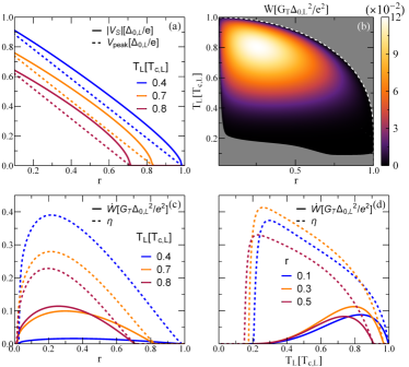
Figure 2: (color online). Thermoelectric figures of merit for a SIS junction. (a) Seebeck voltage vs $r$ for $T_{\rm R}=0.01T_{\rm c,R}$ and some values of $T_{\rm c,L}$ (solid). The voltage corresponding to the singularity matching peak is displayed for a comparison (dashed). (b) Density plot of the thermoelectric power $\dot{W}=-IV$ vs $r$ and $T_{\rm L}$ for $T_{\rm R}=0.01T_{\rm c,L}$. In the gray region the thermoelectric effect is absent, i.e., the junction is dissipative $\dot{W}<0$. The white dashed curve displays the equation $\Delta_{\rm L}(T_{\rm L})=\Delta_{\rm 0,R}$. (c),(d) Cuts of Fig. 2b for particular values of $T_{\rm L}$ and $r$, respectively. The correspondent thermoelectric efficiency $\eta=\dot{W}/\dot{Q}_{\rm L}$ is plotted with dashed lines.

Figure 2a displays $|V_{\rm S}|$ as a function of $r$ for $T_{\rm R}=0.01T_{\rm c,R}$ and some values of $T_{\rm L}>T_{\rm R}$ (solid lines). The curves show some characteristic features: i) for a given $T_{\rm L}$, $|V_{\rm S}|$ decreases monotonically with $r$ and it is zero when $r$ is larger than some critical value (depending on $T_{\rm L}$), ii) for a given $r$, $|V_{\rm S}|$ decreases when the temperature $T_{\rm L}$, that is proportional to the temperature difference $\Delta T$, is increased, something that differ with the usual linear thermoelectricity. These features can be qualitatively understood by comparing $V_{\rm S}$ with the matching peak value $V_{\rm peak}=[\Delta_{\rm L}(T_{\rm L})-\Delta_{\rm R}(T_{\rm R})]/e$ (dashed curves in Fig. 2a). In fact, the magnitude of $V_{\rm S}$ is correlated to $V_{\rm peak}$, i.e., $|V_{\rm S}|\geq V_{\rm peak}$ when there is thermoelectricity (see Fig. 1b,c). By definition, for a given $T_{\rm L}$, $V_{\rm peak}$ decreases almost linearly with $r$, i.e., $eV_{\rm peak}/\Delta_{\rm 0,L}\sim\Delta_{\rm L}(T_{\rm L})/\Delta_{\rm 0,L}-r$. This explains also the temperature evolution, since $\Delta_{\rm L}(T_{\rm L})$ is a monotonically decreasing function. In particular, when $r$ is larger than a critical value depending on $T_{\rm L}$, i.e., $r\gtrsim\Delta_{\rm 0,R}/\Delta_{\rm L}(T_{\rm L})$, $V_{\rm S}$ goes to zero since $\Delta_{\rm L}(T_{\rm L})<\Delta_{\rm R}(T_{\rm R})$, i.e., there is no thermoelectricity. For $r=0.3$, an effective nonlinear Seebeck coefficient $\mathcal{S}=V_{\rm S}/\Delta T$ can reach values as large as $\sim 0.8\Delta_{\rm 0,L}/(0.4eT_{\rm c,L})=2\times 1.764k_{\rm B}/e\sim 300\mu$V/K.

Now, we consider the thermo-electric power $\dot{W}=-IV$. For simplicity, we evaluate it at $V_{\rm peak}$, where it is approximately maximum SM , namely $-I(V_{\rm peak})V_{\rm peak}\sim\max_{V}(-IV)$. Figure 2b displays the density plot of $\dot{W}$ as a function of $r$ and $T_{\rm L}$ for $T_{\rm R}=0.01T_{\rm c,L}$. The thermo-electric power is absent if $T_{\rm L}\leq 0.1T_{\rm c,L}$, irrespectively of $r$. Furthermore, it is zero when $\Delta_{\rm L}(T_{\rm L})<\Delta_{\rm 0,R}$ (the dashed white line in Fig. 2b displays the curve $\Delta_{\rm L}(T_{\rm L})=\Delta_{\rm 0,R}$). The maximum value of $\dot{W}$ is obtained at $r\sim 0.25$ and $T_{\rm L}=0.8T_{\rm c,L}$ and it yields $\dot{W}_{\rm max}\sim 0.11~{}G_{\rm T}\Delta_{\rm 0,L}^{2}/e^{2}$. For an aluminum based ($\Delta_{\rm 0,L}/e\sim 200\mu$V) tunnel junction with $G_{\rm T}=(1{\rm k}\Omega)^{-1}$, the maximum is $\dot{W}_{\rm max}\sim 4$ pW.

For a better characterization, we consider cuts of Fig. 2b for specific values of $T_{\rm L}$ (solid curves in Fig. 2c) and $r$ (solid curves in Fig. 2d). In both the panels, we add the corresponding thermoelectric efficiency $\eta=\dot{W}/\dot{Q}_{\rm L}$ (dashed curves). Interestingly, the highest absolute efficiency with respect to $r$ is obtained almost in correspondence of the maximum power $\eta_{\rm max}\sim 0.4$ (see Fig. 2c). Conversely, the best condition for $\eta$ as a function of $T_{\rm L}$ does not coincide with the condition for maximum power (see Fig. 2d), although $\eta$ is quite high even at the best condition in terms of power $\eta_{\dot{W}_{\rm max}}=\eta(T_{\rm L}=0.8T_{\rm c,L})\sim 0.22$ (orange line in Fig. 2d).

Spontaneous symmetry breaking.

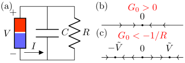
Figure 3: (color online). (a) Circuital scheme: the junction is a nonlinear element with characteristic $I(V,T_{\rm L},T_{\rm R})$ and capacitance $C$, connected to a generic load R. (b)-(c) Phase portrait for the voltage dynamics across the system. (b) In the absence of thermoelectricity, $G_{0}>0$ and the voltage relaxes to 0, due to the dissipation in the load. (c) In the presence of thermoelectricity and for $G_{0}<-1/R$, the zero-voltage solution is unstable and a voltage, either $\pm\tilde{V}$, spontaneously develops across the junction.

Here we discuss the experimental consequences of thermoelectricity in terms on the junction’s dynamics. We consider a minimal circuital setup, displayed in Fig. 3a. The junction is modeled as a nonlinear element of characteristic $I(V,T_{\rm L},T_{\rm R})$ and capacitance $C$, in parallel with a load external circuit of resistance $R$. The evolution is obtained by requiring the current conservation in the circuit,

$$I(V,T_{\rm L},T_{\rm R})=-C\dot{V}-\frac{V}{R},$$ (4)

where the dot denotes the time ($t$) derivative. The stationary points are obtained by setting $\dot{V}=0$ in Eq. 4 and read $V(t)=\tilde{V}$, where $\tilde{V}$ is a solution of the implicit equation $RI(\tilde{V},T_{\rm L},T_{\rm R})+\tilde{V}=0$. Since $I(V,T_{\rm L},T_{\rm R})=-I(-V,T_{\rm L},T_{\rm R})$, the equation has an odd number of solutions and $\tilde{V}=0$ is always a solution, irrespectively of $R,T_{\rm L},T_{\rm R}$. The stability of these solutions can be acquired by linearizing Eq. 4, namely $\dot{v}=-C^{-1}[G(\tilde{V})+1/R]v$, where $v=V-\tilde{V}$ and $G(\tilde{V})=dI/dV|_{V=\tilde{V}}$. The solution is stable if the term in the square bracket is positive and unstable otherwise.

In the absence of thermoelectricity, $IV\geq 0$ and the zero-bias conductance of the junction is positive $G_{0}\geq 0$. Thus, $\tilde{V}=0$ is the unique solution of Eq. 4 and it is stable (see Fig. 3b). Conversely, when we apply a temperature gradient and the SIS junction displays thermoelectricity, $G_{0}<0$ (see Eq. 3), and additional solutions at finite voltages are possible. In particular, for sufficiently large values of the load, such as $R>-G_{0}^{-1}$ there are three solutions $V=0,\pm\tilde{V}$, and $G(\pm\tilde{V})>0$. As a consequence, any voltage signal across the device evolves toward one of the two values $\pm\tilde{V}$, depending on the initial conditions (see Fig. 3c). Namely, the combination of a sufficiently strong thermal gradient and the voltage polarization imposed by the external circuit leads to a spontaneous breaking of EH symmetry. Moreover, the bi-stability of the stationary voltage may be used to design a volatile thermo-electric memory or a switch SM . In a more general setting which includes inductive effects, the instability of the zero-voltage state can generate also a self-sustained oscillatory dynamics SM ; Goupil et al. (2016); Alicki et al. (2017).

Conclusions. In summary, we discussed a general thermo-electric effect occurring in systems with EH symmetry in the nonlinear regime. For a two-terminals tunneling system, two sufficient conditions are required for thermoelectricity: i) the hot electrode has a gapped DoS, ii) the cold electrode has a locally monotonically decreasing DoS. In particular, we investigated a prototype system: a tunnel junctions between two different BCS superconductors. We displayed the relevant figures of merit and showed that a thermoelectric voltage spontaneously develops across the system, under proper conditions. Our results may be extended to different classes of materials, including hybrid ferromagnetic-superconducting junctions or low-dimensional quantum systems (dots or wires). This work can represent a promising step in the exploration of thermo-electric effects in the nonlinear regime.