TUM-HEP-1222/19
September 09, 2019

Wino potential and Sommerfeld effect at NLO

Martin Beneke,^a Robert Szafron,^a Kai Urban^a

^aPhysik Department T31,
James-Franck-Straße 1, Technische Universität München,
D–85748 Garching, Germany

We calculate the SU(2)$\times$U(1) electroweak static potential between a fermionic triplet in the broken phase of the Standard Model in the one-loop order (NLO). The one-loop correction provides the leading non-relativistic correction to the large Sommerfeld effect in the annihilation of wino or wino-like dark matter particles $\chi^{0}$. We find sizeable modifications of the $\chi^{0}\chi^{0}$ annihilation cross section and determine the shifts of the resonance locations due to the loop correction to the wino potential.

1 Introduction

It is by now well-known that the Sommerfeld effect due to the electroweak Yukawa force [1, 2, 3] can lead to a dramatic enhancement of the annihilation cross section of two dark matter (DM) particles if their mass is in the TeV range. Contrary to the classic Sommerfeld effect for massless gauge boson exchange in QED and QCD, which rises as $1/v$ as the relative velocity of the annihilating particles decreases, the enhancement due to the Yukawa force saturates at small velocities, except near isolated resonances. These occur at dark matter mass values, when a zero-energy bound-state develops in the spectrum. The phenomenon is quite general and also appears for lighter DM, if there is a force carrier with even smaller mass [4]. Furthermore, if the DM particle is part of a multiplet with a small mass splitting, the effect depends sensitively on the mass difference [5].

Its main interest is nevertheless due to the fact that it is a generic feature of the classic WIMP DM particle, where it arises from the well-established Standard Model (SM) interactions. Thus, it appears in the so-called minimal models [6] and for TeV scale MSSM WIMPs (see, for example, [7, 8, 9]). The Sommerfeld effect is particularly important for the annihilation rates and relic density of the pure wino, an electroweak triplet of fermions of which the electrically neutral member is the DM particle [2, 3, 6, 10, 11, 12], or a mixed but dominantly wino state [13, 14]. The pure wino (“wino” in the following) model has become a test case for the quantitative understanding of large electroweak corrections in the annihilation of TeV scale DM particles. In view of the possible detection or exclusion of the wino particle through measurements of high-energy cosmic rays, the wino annihilation rate into photons is of particular interest. Here electroweak perturbation theory breaks down due to electroweak Sudakov logarithms, which must be summed in addition to the Sommerfeld corrections. Recent work on exclusive and semi-inclusive photon yields has shown that Sudakov logarithms can be controlled with 1% accuracy with NLL’ resummation [15, 16, 17]. At this level of precision, the treatment of the Sommerfeld effect should be revisited, since, up to the present, all calculations have been done with the tree-level exchange potential, which corresponds to the leading-order (LO) approximation in non-relativistic effective field theory (EFT) for the DM particle [18, 19, 8].

In this paper we compute the one-loop corrections to the wino potential and discuss its effect on the wino pair annihilation cross section to photons, $\chi^{0}\chi^{0}\to\gamma+X$. We recall [1, 2, 3] that the LO potential is given by the matrix

$$V_{\rm LO}(r)=\left(\begin{array}[]{cc}\displaystyle 0&\displaystyle\quad-\sqrt{2}\,\alpha_{2}\,\frac{e^{-m_{W}r}}{r}\\ \displaystyle-\sqrt{2}\,\alpha_{2}\,\frac{e^{-m_{W}r}}{r}&\displaystyle\quad-\frac{\alpha}{r}-\alpha_{2}\,c_{W}^{2}\,\frac{e^{-m_{Z}r}}{r}\end{array}\right).$$ (1)

The $IJ$ entry refers to the non-relativistic scattering of wino two-particle states $I\to J$ with $I,J=1,2$ referring to $\chi^{0}\chi^{0}$ and $\chi^{+}\chi^{-}$, respectively. The above matrix describes the scattering of electrically neutral two-particle states in a ${}^{1}S_{0}$ spin-angular-momentum configuration, since the spin-1 configuration is forbidden due to the Majorana nature of the $\chi^{0}$. One might expect the one-loop correction to the potential to be small due to the smallness of the SU(2)$\times$U(1) couplings. However, we shall see that over most of the interesting wino mass range from 1 to 10 TeV, the effect on the annihilation cross section is significantly larger than the typical $3\%$ of an electroweak quantum effect.

In the following we give only a brief overview of technical details of the computation and then present results for the potential and the annihilation cross section into photons. An NLO Sommerfeld calculation of the relic density involves the potentials for all coannihilation channels. We leave this to a longer and more technical paper.

2 Technical details

The Sommerfeld effect is a low-energy phenomenon that appears for non-relativistic DM particles. A systematic treatment of non-relativistic effects can be given in non-relativistic and potential-non-relativistic DM EFT [18, 8]. The potential appears in the effective Lagrangian

$$\mathcal{L}_{\rm PNRDM} = \sum_{i}\chi_{vi}^{\dagger}(x)\left(iD^{0}(t,\mathbf{0})-\delta m_{i}+\frac{\bm{\partial}^{2}}{2m_{\chi}}\right)\chi_{vi}(x)$$ (2)

$$-\,\sum_{\{i,j\},\{k,l\}}\int d^{3}\mathbf{r}\,V_{\{ij\}\{kl\}}(r)\,\chi_{vk}^{\dagger}(t,\mathbf{x})\chi_{vl}^{\dagger}(t,\mathbf{x}+\mathbf{r})\chi_{vi}(t,\mathbf{x})\chi_{vj}(t,\mathbf{x}+\mathbf{r})\quad$$

as an instantaneous but spatially non-local interaction of four non-relativistic wino fields $\chi_{vi}$ where $i=0,+,-$. $\delta m_{i}$ denotes the small mass splitting between the $\chi^{-}$ and the $\chi^{0}$ state.

Standard non-relativistic power counting for the wino assumes $\alpha_{2}\sim v\sim m_{W}/m_{\chi}$, although it is then possible to consider $v\ll\alpha_{2}$. The potential generated by tree-level gauge boson exchange is then a leading-order interaction – as large as the kinetic term. Treating this interaction as part of the unperturbed Lagrangian and solving the corresponding Schrödinger equation gives the LO Sommerfeld effect. Similarly, the radiative mass splitting $\delta m_{i}\sim m_{W}\alpha_{2}$ at the one-loop order is of the same order as $\partial_{0}\sim E\sim m_{\chi}v^{2}$, and therefore relevant at LO. NLO corrections, that is, corrections suppressed by one power of $\alpha_{2}$, $v$ or $m_{W}/m_{\chi}$ to the above Lagrangian arise from a) the two-loop correction to the mass splitting, which is known [20, 21], b) the one-loop correction to the Yukawa/Coulomb potential (1), which is the subject of this paper, and, possibly from c) potentials with more singular short-distance behaviour than $1/r$, similar to the massless gauge boson case, and d) ultrasoft gauge-boson radiation. However, the latter two effects do not appear at NLO for the same reason as in QCD and QED. Note that there exist of course NLO corrections to the annihilation process (see, for example, [22, 16, 17]), but here we are concerned with non-relativistic effects.

The potential is technically a matching coefficient between non-relativistic and potential non-relativistic DM EFT. It is obtained from the wino-wino scattering amplitude $i\,T^{\chi\chi\to\chi\chi}_{ijkl}(\bm{q})$ at small momentum transfer $\bm{q}$. At the one-loop order, the matching coefficient is extracted from the soft region in the method-of-region expansion [23], which is automatic, if one replaces the non-relativistic wino propagators by static propagators $i/p^{0}$, and picks up the poles in the loop-momentum zero-component $k^{0}$ from the gauge-boson propagators. The coordinate-space potentials follow by taking the Fourier transform

$$V_{\{ij\}\{kl\}}(r)=\int\frac{d^{3}\bm{q}}{(2\pi)^{3}}\,e^{i\bm{q}\cdot\bm{x}}\,i\,T^{\chi\chi\to\chi\chi}_{ijkl}(\bm{q}^{2})\,,$$ (3)

where $r\equiv|\bm{x}\,|$. From the identity

$$\int\frac{d^{3}\bm{q}}{(2\pi)^{3}}\,e^{i\bm{q}\cdot\bm{x}}\,\frac{1}{\bm{q}^{2}+m^{2}}=\frac{e^{-mr}}{4\pi r}\,,$$ (4)

one recognizes the well-known Yukawa-like potential for amplitudes with exchange of a force carrier of mass $m$.

Figure 1: Feynman diagrams for the $\chi^{+}\chi^{-}\to\chi^{+}\chi^{-}$ scattering channel (excluding field renormalization, counterterm and tadpole diagrams). Arrows on propagators indicate charge flow. For the $\chi^{0}\chi^{0}\to\chi^{0}\chi^{0}$ channel, of the above diagrams only the box and crossed box with $W$-exchange exist and cancel against each other. In the $\chi^{0}\chi^{0}\to\chi^{+}\chi^{-}$ channel, the same topologies as above are possible (with different bosons such that charge flow is respected), except for the crossed box diagram.

Following this procedure, the calculation of the one-loop correction to the wino potential is standard, and involves the Feynman diagrams shown in Figure 1. We performed the calculation in general covariant gauge with different gauge parameters $\xi$ for the $W$-, $Z$-boson and photon, and find that the result does not depend on the gauge-fixing parameters, as required. The diagrams are reduced to a few master integrals, which are then calculated analytically. For the gauge boson self-energy diagrams in general covariant gauge we used FeynArts [26], FORMCalc [27] and Package-X [28] and checked the result in Feynman gauge against [24]. We adopted the standard on-shell renormalization scheme for the electroweak parameters, consisting of $m_{W}$, $m_{Z}$ and the QED coupling $\alpha_{\rm{OS}}(m_{Z})$, since the dominant scale of the Sommerfeld effect is the electroweak scale. We further checked that as $r\ll 1/m_{W}$, the correction coincides with the one-loop Coulomb potential in the massless theory after switching to the $\overline{\rm MS}$ renormalization scheme for the couplings. As a final check, we confirm the previously known expression for the singlet Yukawa potential in a Higgsed SU(2) theory [29, 30] by taking the limit $m_{W}\to m_{Z}$ and hence $s_{W}\to 0,c_{W}\to 1$. More precisely, we confirmed the non-renormalized potential (Eq. 16 in [29]) analytically. The renormalized result was not compared, as the renormalization scheme was not fully specified.

3 NLO potential

3.1 Result

We obtain an analytic expression for the one-loop wino potential in momentum space. The Fourier transform (3) to the coordinate space potential is performed analytically where possible, however, for a few of the momentum-space functions at the one-loop order, we did not find the Fourier transform in a closed form, and leave it as a one-dimensional integral. The momentum-space potential is a lengthy expression, which will be given elsewhere, together with the potentials for the charged and spin-triplet channels required for relic density computations. Instead we provide a handy fitting function for the coordinate-space potential in the ${}^{1}S_{0}$ channel for charge-zero wino-wino scattering, which corrects (1) by

$$\delta V(r)=\left(\begin{array}[]{cc}\displaystyle 0&\sqrt{2}\,\delta V_{(00)\to(+-)}\\ \sqrt{2}\,\delta V_{(00)\to(+-)}&\delta V_{(+-)\to(+-)}\end{array}\right),$$ (5)

and can be easily implemented in numerical Sommerfeld codes. We note that the potential in the neutral channel $\chi^{0}\chi^{0}\to\chi^{0}\chi^{0}$ vanishes, because the only two contributing one-loop diagrams, the box and the crossed box diagram, cancel each other.

Fitting function in the charged channel

We use $x=m_{W}r$, and define

$$\delta V^{\text{fit}}_{(+-)\to(+-)} =\frac{\delta V^{r\to\infty}_{(+-)\to(+-)}}{1+\frac{32}{11}x^{-\frac{22}{9}}}+\frac{\delta V^{r\to 0}_{(+-)\to(+-)}}{1+\frac{7}{59}x^{\frac{61}{29}}}+\frac{\alpha}{r}\left[\frac{-\frac{1}{30}+\frac{4}{135}\log x}{1+\frac{58}{79}x^{-\frac{17}{15}}+\frac{1}{30}x^{\frac{119}{120}}+\frac{8}{177}x^{\frac{17}{8}}}\right].$$ (6)

The fitting function is constructed from the asymptotic behaviours

$$\delta V^{r\to 0}_{\chi_{+}\chi_{-}\to\chi_{+}\chi_{-}}(r) = \frac{\alpha_{2}^{2}}{2\pi r}\left(-\beta_{0,\text{SU(2)}}\,\ln(m_{W}r)+\frac{1960}{433}\right),$$ (7)

$$\delta V^{r\to\infty}_{\chi_{+}\chi_{-}\to\chi_{+}\chi_{-}}(r) = \frac{\alpha^{2}}{2\pi r}\,(-\beta_{0,\rm{em}})\left(\gamma_{E}+\ln(m_{Z}r)\right)$$ (8)

at large and small distances and an interpolating term. The coefficients are rationalized to provide a compact expression, including the constant term $\frac{1960}{433}$ in (7). $\beta_{0,\text{SU(2)}}=19/6$ and $\beta_{0,\text{em}}=-80/9$ denote the leading-order coefficients of the beta-functions of the SU(2) and electromagnetic couplings, and $\gamma_{E}=0.577215\ldots$ is Euler’s constant. The fitting function approximates the result of the partially numerical Fourier transform to better than $0.1\%$ over the entire distance region of interest, as shown in Figure 2.

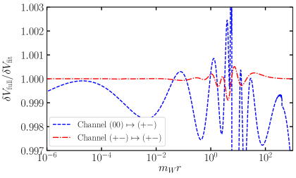
Figure 2: Ratio of the numerical Fourier transform of the potential correction to the fitting function in the variable $x=m_{W}r$ for the channel $(00)\to(+-)$ (blue/dashed) and $(+-)\to(+-)$ (red/dot-dashed). The relative difference is in the permille range.

The rationalized coefficients of the numerical fitting function are given for the following parameters: the on-shell electromagnetic coupling $\alpha\equiv\alpha_{\rm{OS}}(m_{Z})=1/128.943$ at the $Z$-boson mass scale, and the gauge-boson masses $m_{W}=80.385\,\rm{GeV}$ and $m_{Z}=91.1876\,\rm{GeV}$. The cosine of the Weinberg angle and the SU(2) coupling are then determined from $c_{W}=m_{W}/m_{Z}$ and $\alpha_{2}=\alpha_{\rm{OS}}(m_{Z})/s_{W}^{2}=0.0347935$. We also need the top quark and Higgs boson mass, for which we take the on-shell masses $m_{t}=173.1\,\rm{GeV}$ and $m_{h}=125\,\rm{GeV}$. These parameters will also be used in the following discussion. For the calculation of the Sommerfeld enhancement below, we need in addition the two-loop mass splitting $\delta m_{\chi}=164.1\,\rm{MeV}$ between the charged and the neutral component of the wino multiplet. The dependence of the results on the uncertainties in these parameters is small enough to be ignored, except for the top-quark mass, as will be briefly discussed below.

Fitting function in the off-diagonal $(00)\to(+-)$ channel

Because the correction to the potential changes sign in this channel near $x_{0}=m_{W}r_{0}=\frac{555}{94}$, we did not manage with a single fitting function. Instead we use the piecewise expression

$$\delta V^{\text{fit}}_{(00)\to(+-)} =\frac{2595\alpha^{2}_{2}}{\pi r}\times\left\{\begin{array}[]{r}\text{exp}\left[-\frac{79\left(L-\frac{787}{12}\right)\left(L-\frac{736}{373}\right)\left(L-\frac{116}{65}\right)\left(L^{2}-\frac{286L}{59}+\frac{533}{77}\right)}{34\left(L-\frac{512}{19}\right)\left(L-\frac{339}{176}\right)\left(L-\frac{501}{281}\right)\left(L^{2}-\frac{268L}{61}+\frac{38}{7}\right)}\right],\quad x<x_{0}\\[14.22636pt] -\text{exp}\left[-\frac{13267\left(L-\frac{76}{43}\right)\left(L-\frac{28}{17}\right)\left(L+\frac{37}{30}\right)\left(L^{2}-\frac{389L}{88}+\frac{676}{129}\right)}{5\left(L-\frac{191}{108}\right)\left(L-\frac{256}{153}\right)\left(L+\frac{8412}{13}\right)\left(L^{2}-\frac{457L}{103}+\frac{773}{146}\right)}\right],\quad x>x_{0}\end{array}\right.$$ (11)

with $L=\ln x=\ln(m_{W}r)$. Figure 2 shows that the quality of the fitting function is at the few permille level, slightly worse than in the charged channel. At small $r$, one can also use the asymptotic behaviour $\delta V^{r\to 0}_{\chi_{0}\chi_{0}\to\chi_{+}\chi_{-}}(r)=\delta V^{r\to 0}_{\chi_{+}\chi_{-}\to\chi_{+}\chi_{-}}(r)$.

3.2 Discussion

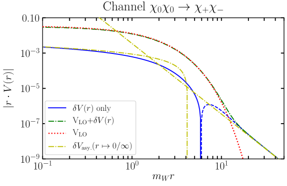
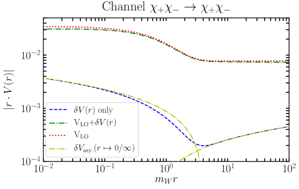
Figure 3: The absolute value of LO and the NLO potential, and of the one-loop correction $\delta V(r)$ together with its asymptotic behaviours, all multiplied by $r$, in the off-diagonal and charged wino-wino scattering channel.

The following discussion of the one-loop corrected wino potential is based on the exact calculation and does not use the fitting functions from above.

The LO and NLO potential, and the NLO correction $\delta V(r)$ are shown in Figure 3 for the off-diagonal and charged wino-wino scattering channel. At small distances, the one-loop correction is governed by the correction (7) to the Coulomb potential of the unbroken SU(2) force, which amounts to about minus $\mathcal{O}(5$-$10\%)$ for $10^{-2}<m_{W}r<1$ relative to the LO potential. At even smaller $r$, the logarithmic growth of the correction, see (7), can be absorbed by using a running SU(2) coupling, rather than the on-shell coupling. The one-loop term $\delta V(r)$ in the off-diagonal $\chi^{0}\chi^{0}\to\chi^{+}\chi^{-}$ scattering channel (upper panel in the Figure) turns from positive to negative for $m_{W}r\geq 6$ and its absolute value exceeds the tree-level potential at large $r$. Contrary to the naive expectation, the large-$r$ asymptotics of the correction is not of the Yukawa form $e^{-m_{W}r}/r$. This can be understood from the fact that the self-energy diagram in Figure (1) probes the transverse gauge-boson self energy $\Pi_{W}(-\bm{k}^{2})$ at $\bm{k}^{2}\ll m_{W}^{2}$ in the large-$r$ limit. Expanding the self-energy resummed gauge-boson propagator $1/(\bm{k}^{2}+m_{W,0}^{2}-\Pi_{W}(-\bm{k}^{2})+\delta m_{W}^{2})$, where $m_{W,0}$ denotes the bare $W$ mass and $\delta m_{W}^{2}$ the on-shell counterterm, around $\bm{k}^{2}=0$, and transforming to coordinate space, we obtain the power-like rather than exponential asymptotic behaviour

$$\delta V^{r\to\infty}_{\chi_{0}\chi_{0}\to\chi_{+}\chi_{-}}(r) = -\frac{9\alpha_{2}^{2}}{\pi m_{W}^{4}r^{5}}\,,$$ (12)

which describes the tail of the NLO potential in the $\chi^{0}\chi^{0}\to\chi^{+}\chi^{-}$ scattering channel well for $m_{W}r>20$.

The behaviour of the charged scattering channel (lower panel in Figure 3) at large distances is simpler, since the asymptotic behaviour becomes again Coulombic due to the dominance of massless photon exchange over the exponentially decaying terms generated by diagrams with $W$ and $Z$ exchange. Except in an intermediate region around $m_{W}r\sim 1$, the potential is described well by the asymptotic expressions (7), (8). The correction is around $-4\%$ at $m_{W}r=10$, and grows logarithmically with the QED beta-function generated by the massless fermions of the SM.

4 Sommerfeld effect and annihilation cross section

We calculate the Sommerfeld effect at NLO by solving the Schrödinger equation with the NLO wino potential employing the variable phase method described in [8]. To display the NLO effect from the potential, we calculate the semi-inclusive $\chi^{0}\chi^{0}$ annihilation cross section into $\gamma+X$ with the same tree-level approximation

$$\Gamma=2\,\Gamma_{\gamma\gamma}+\Gamma_{\gamma Z}=\frac{2\pi\alpha_{2}^{2}}{m_{\chi}^{2}}\left(\begin{array}[]{cc}\displaystyle 0&0\\ 0&s_{W}^{2}\end{array}\right)$$ (13)

to the short-distance annihilation matrix.

Figure 4: $\sigma v$ calculated with the LO (solid/blue) and the NLO (dash-dotted/red) potential. The lower panel shows the ratio of the NLO to LO result with dark (light) grey bands to visualize the range where the correction stays below 20% (40%).

In the upper panel of Figure 4 we show $\sigma v$, the annihilation cross section times velocity calculated with the LO (solid/blue) and the NLO (dash-dotted/red) potential in the mass range $m_{\chi}=0.5\ldots 20$ TeV for the DM particle, which covers the onset of the Sommerfeld enhancement at small masses and the first two resonances. We recall that the observed relic density is achieved for a wino mass of $2.88$ TeV [13]. That the NLO correction is visible on a logarithmic plot already indicates that it is significant. The location of the first two Sommerfeld resonances shifts from $2.283$ ($8.773$) TeV at LO to $2.419$ ($9.355$) TeV at NLO. Since the resonances both move to larger masses, the NLO correction changes sign in the mass range between the resonances and always remains sizeable. This can be seen in the subtended lower panel of Figure 4, which displays the ratio of the NLO to LO annihilation cross section. The ratio evidently blows up near the resonances due to the location-shift, but it is larger than 20% for wide mass ranges, and always larger than the typical 3% for an electroweak loop correction.

For completeness, we show in Figure 5 the accuracy of the annihilation cross section when instead of the exact computation of the NLO potential, the fitting functions are used. The error is at most 0.3% near the first resonance and usually substantially smaller. The first (second) resonance position changes by only 0.1 GeV (0.2 GeV).

The above results depend on the value of the top quark mass through the gauge boson self energies. We adopted the on-shell mass, since the characteristic scale for the Sommerfeld effect is the electroweak scale. If instead we choose the $\overline{\rm MS}$ mass $\overline{m}_{t}(\overline{m}_{t})=163.35$ GeV, the NLO resonances are located at $2.408$ TeV, $9.311$ TeV, respectively. This amounts to a change of about 8% in the size of the shifts from LO to NLO. The overall picture remains unaffected.

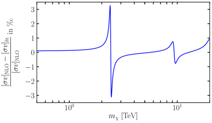
Figure 5: Relative error in permille of the Sommerfeld enhanced cross section using the full NLO potential vs. the fitting function for the relevant range of values of DM mass $m_{\chi}$.

In summary, we computed the NLO correction to the wino potential. We find that the Sommerfeld resonances are shifted by about 6% to larger values, from 2.283 TeV to 2.419 TeV for the first resonance, and find sizeable corrections over the entire mass range relevant for wino-like DM. This effect is generally larger than a typical electroweak loop correction and should be included in precision predictions of annihilation rates in the wino model, such as [15, 16, 17]. Furthermore, the size of the effect suggests further investigation of its relevance for the relic DM abundance, which requires the calculation of the NLO potentials in all coannihilation channels.

Acknowledgements

This work was supported in part by the DFG Collaborative Research Centre “Neutrinos and Dark Matter in Astro- and Particle Physics” (SFB 1258).

References

- [1] J. Hisano, S. Matsumoto and M. M. Nojiri, Explosive dark matter annihilation, Phys. Rev. Lett. 92 (2004) 031303, [hep-ph/0307216].
- [2] J. Hisano, S. Matsumoto, M. M. Nojiri and O. Saito, Non-perturbative effect on dark matter annihilation and gamma ray signature from galactic center, Phys. Rev. D71 (2005) 063528, [hep-ph/0412403].
- [3] J. Hisano, S. Matsumoto, M. Nagai, O. Saito and M. Senami, Non-perturbative effect on thermal relic abundance of dark matter, Phys. Lett. B646 (2007) 34–38, [hep-ph/0610249].
- [4] N. Arkani-Hamed, D. P. Finkbeiner, T. R. Slatyer and N. Weiner, A Theory of Dark Matter, Phys. Rev. D79 (2009) 015014, [0810.0713].
- [5] T. R. Slatyer, The Sommerfeld enhancement for dark matter with an excited state, JCAP 1002 (2010) 028, [0910.5713].
- [6] M. Cirelli, A. Strumia and M. Tamburini, Cosmology and Astrophysics of Minimal Dark Matter, Nucl.Phys. B787 (2007) 152–175, [0706.4071].
- [7] A. Hryczuk, R. Iengo and P. Ullio, Relic densities including Sommerfeld enhancements in the MSSM, JHEP 03 (2011) 069, [1010.2172].
- [8] M. Beneke, C. Hellmann and P. Ruiz-Femenia, Non-relativistic pair annihilation of nearly mass degenerate neutralinos and charginos III. Computation of the Sommerfeld enhancements, JHEP 05 (2015) 115, [1411.6924].
- [9] M. Beneke, C. Hellmann and P. Ruiz-Femenia, Heavy neutralino relic abundance with Sommerfeld enhancements - a study of pMSSM scenarios, JHEP 03 (2015) 162, [1411.6930].
- [10] A. Hryczuk and R. Iengo, The one-loop and Sommerfeld electroweak corrections to the Wino dark matter annihilation, JHEP 01 (2012) 163, [1111.2916].
- [11] J. Fan and M. Reece, In Wino Veritas? Indirect Searches Shed Light on Neutralino Dark Matter, JHEP 10 (2013) 124, [1307.4400].
- [12] T. Cohen, M. Lisanti, A. Pierce and T. R. Slatyer, Wino Dark Matter Under Siege, JCAP 1310 (2013) 061, [1307.4082].
- [13] M. Beneke, A. Bharucha, F. Dighera, C. Hellmann, A. Hryczuk, S. Recksiegel et al., Relic density of wino-like dark matter in the MSSM, JHEP 03 (2016) 119, [1601.04718].
- [14] M. Beneke, A. Bharucha, A. Hryczuk, S. Recksiegel and P. Ruiz-Femenia, The last refuge of mixed wino-Higgsino dark matter, JHEP 01 (2017) 002, [1611.00804].
- [15] G. Ovanesyan, N. L. Rodd, T. R. Slatyer and I. W. Stewart, One-loop correction to heavy dark matter annihilation, Phys. Rev. D95 (2017) 055001, [1612.04814].
- [16] M. Beneke, A. Broggio, C. Hasner and M. Vollmann, Energetic -rays from TeV scale dark matter annihilation resummed, Phys. Lett. B786 (2018) 347–354, [1805.07367].
- [17] M. Beneke, A. Broggio, C. Hasner, K. Urban and M. Vollmann, Resummed photon spectrum from dark matter annihilation for intermediate and narrow energy resolution, JHEP 08 (2019) 103, [1903.08702].
- [18] M. Beneke, C. Hellmann and P. Ruiz-Femenia, Non-relativistic pair annihilation of nearly mass degenerate neutralinos and charginos I. General framework and S-wave annihilation, JHEP 03 (2013) 148, [1210.7928].
- [19] C. Hellmann and P. Ruiz-Femenia, Non-relativistic pair annihilation of nearly mass degenerate neutralinos and charginos II. P-wave and next-to-next-to-leading order S-wave coefficients, JHEP 08 (2013) 084, [1303.0200].
- [20] Y. Yamada, Electroweak two-loop contribution to the mass splitting within a new heavy SU(2)(L) fermion multiplet, Phys. Lett. B682 (2010) 435–440, [0906.5207].
- [21] M. Ibe, S. Matsumoto and R. Sato, Mass Splitting between Charged and Neutral Winos at Two-Loop Level, Phys. Lett. B721 (2013) 252–260, [1212.5989].
- [22] M. Baumgart, T. Cohen, I. Moult, N. L. Rodd, T. R. Slatyer, M. P. Solon et al., Resummed Photon Spectra for WIMP Annihilation, JHEP 03 (2018) 117, [1712.07656].
- [23] M. Beneke and V. A. Smirnov, Asymptotic expansion of Feynman integrals near threshold, Nucl. Phys. B522 (1998) 321–344, [hep-ph/9711391].
- [24] A. Denner, Techniques for calculation of electroweak radiative corrections at the one loop level and results for W physics at LEP-200, Fortsch. Phys. 41 (1993) 307–420, [0709.1075].
- [25] J. Fleischer and F. Jegerlehner, Radiative Corrections to Higgs Decays in the Extended Weinberg-Salam Model, Phys. Rev. D23 (1981) 2001–2026.
- [26] T. Hahn, Generating Feynman diagrams and amplitudes with FeynArts 3, Comput. Phys. Commun. 140 (2001) 418–431, [hep-ph/0012260].
- [27] T. Hahn and M. Perez-Victoria, Automatized one loop calculations in four-dimensions and D-dimensions, Comput. Phys. Commun. 118 (1999) 153–165, [hep-ph/9807565].
- [28] H. H. Patel, Package-X 2.0: A Mathematica package for the analytic calculation of one-loop integrals, Comput. Phys. Commun. 218 (2017) 66–70, [1612.00009].
- [29] M. Laine, The Renormalized gauge coupling and nonperturbative tests of dimensional reduction, JHEP 06 (1999) 020, [hep-ph/9903513].
- [30] Y. Schröder, The Static potential in QCD, Ph.D. thesis, Hamburg U., 1999.