Deviations from Gaussianity in deterministic discrete time dynamical systems

Abstract

In this paper we examine the deviations from Gaussianity for two types of random variable converging to a normal distribution, namely sums of random variables generated by a deterministic discrete time map and a linearly damped variable driven by a deterministic map. We demonstrate how Edgeworth expansions provide a universal description of the deviations from the limiting normal distribution. We derive explicit expressions for these asymptotic expansions and provide numerical evidence of their accuracy.

1 Introduction

Randomness provides a powerful way of describing the large-scale behaviour of many systems in the natural and man-made world. Well-known examples are Brownian particle motion, price evolution on financial markets and the evolution of the Earth’s climate. However, many of these systems are described by deterministic dynamical systems on small scales. A natural question is then how randomness arises from deterministic dynamics.

One much-explored way in which random variable can arise from deterministic dynamical systems is through variations of the central limit theorem. In such theorems, many nearly independent contributions are added or integrated over to result in a Gaussian random variable. This principle has for example been explored for systems with a bath of a large number of deterministic oscillators [8]. Another way to obtain sums of nearly independent contributions is to sum over time series of sufficiently mixing dynamical systems. The evolution is completely deterministic, with the only randomness appearing through the initial conditions. This approach has been investigated for discrete time dynamical systems in [5, 14, 21]. An extension of this case can be found in the study of slow-fast dynamical systems where instead of simply summing the output of a dynamical system the slow variable has a non-trivial dynamics of its own. This setting has been studied in [15, 9, 13].

In these theorems we have to consider specific limits, for example, taking the number of oscillators, the length of  sums or the time scale separation to inifity. Such conditions are of course never fulfilled in reality. Therefore, the distributions observed in a physical system will deviate from the limiting distribution predicted by theory. These deviations can in many cases be successfully described by Edgeworth expansions, which provide correction terms to the limiting distribution [7, 11, 18, 19]. Edgeworth expansions have furthermore been used to develop reduced order models for slow-fast dynamical systems [20].

Here we consider two applications of Edgeworth expansions. First of all, we describe a method to derive the Edgeworth coefficients of sums of dependent random variables. We corroborate our results by numerical experiments. Secondly, we show that some recent results on approximations of invariant distributions of slow-fast discrete maps are in fact a specific case of the Edgeworth expansion.

The article is structured as follows. In Section 2 we give a brief overview of central limit theorems and the Edgeworth expansion. In Section 3 we examine sums of time series of a deterministic dynamical system with random initial conditions. In Section 4 we study a type of slow-fast dynamical system with linear damping of the slow variable. We show that the deviations of the invariant measure of the slow variable can effectively be described by an Edgeworth expansion.

2 Central limit theorems and Edgeworth expansions

The convergence of appropriately normalized sums of random variables to Gaussian, Poisson or other infinitely divisible distributions is an important topic in probability theory and dynamical systems theory. Theorems showing such convergence are known as central limit theorems (CLT). A CLT holds for a sequence of random variables $z_{i}$ with $i\in\mathbbm{N}$ and $\mathbbm{E}[z_{i}]=0$ if $x_{n}:=\frac{1}{\sqrt{n}}\sum_{i=1}^{n}z_{i}$ converges in distribution to a normal distribution $\mathcal{N}_{0,\sigma^{2}}$ with mean $0$ and variance $\sigma^{2}$ as $n\rightarrow\infty$.

If $x_{n}$ converges to a normal distribution $\mathcal{N}_{0,\sigma^{2}}$ the variance $\sigma^{2}$ is given by $\sigma^{2}=\lim_{n\rightarrow\infty}\mathbbm{V}[x_{n}]$, with $\mathbbm{V}[x_{n}]$ the variance of $x_{n}$. For a stationary generating process $z_{i}$, we have

$$\mathbbm{V}[x_{n}] := \mathbbm{E}[x_{n}^{2}]=\frac{1}{n}\sum_{i=0}^{n-1}\sum_{j=0}^{n-1}\mathbbm{E}[z_{i}z_{j}]$$

$$= \mathbbm{E}[z^{2}_{1}]+2\frac{n-1}{n}\mathbbm{E}[z_{1}z_{2}]+2\frac{n-2}{n}\mathbbm{E}[z_{1}z_{3}]+\ldots+2\frac{1}{n}\mathbbm{E}[z_{1}z_{n}],$$

where the last equality holds by stationarity of the sequence $z_{i}$. Therefore $\sigma^{2}$ is determined by the correlation structure of $z_{i}$ as

$$\sigma^{2} = \mathbbm{E}[z^{2}_{1}]+2\sum_{i=2}^{\infty}\mathbbm{E}[z_{1}z_{i}].$$ (1)

This expression is sometimes referred to as the Green-Kubo formula.

Central limit theorems have been shown to hold for i.i.d random variables [6], independent but non-identical random variables [4], weakly dependent random variables [12] and deterministic discrete time maps [5, 14, 21, 1, 16]. In the case of deterministic maps randomness is introduced by a random choice of the initial condition.

Formally, the CLT can be derived by considering the characteristic function $\chi_{n}(\theta):=\mathbbm{E}[e^{i\theta x_{n}}]$. By Taylor expanding $\ln\chi_{n}$ in $\theta$ we have that

$$\ln\chi_{n}(\theta) = \sum_{k=0}^{\infty}\frac{c_{n}^{(k)}}{k!}(i\theta)^{k}$$

where $c_{n}^{(k)}$ is the $k$-th cumulant of $X_{n}$, satisfying the recursive relation

$$c^{(k)}_{n} = m^{(k)}_{n}-\sum_{l=1}^{k-1}\binom{k-1}{l-1}m^{(k-l)}_{n}c^{(l)}_{n}\,,$$

where $m_{n}^{(k)}$ is the $k$-th central moment of $x_{n}$: $m_{n}^{(k)}:=\mathbbm{E}\left[x_{n}^{k}\right]$ If it can be demonstrated that $c_{n}^{(2)}\rightarrow\sigma^{2}$ and $c_{n}^{(k)}\rightarrow 0$ for $k\geqslant 3$ then $\chi_{n}\rightarrow e^{-\frac{\sigma^{2}}{2}\theta^{2}}$, the characteristic function of the normal distribution $\mathcal{N}_{0,\sigma^{2}}$. The convergence in distribution of $x_{n}$ then follows from Lévy’s continuity theorem [6].

2.1 Deviations from the limiting distribution

The formal derivation of the CLT in the previous section can be extended to provide more details on the way in which the limiting distribution is approached. This results in a so-called Edgeworth expansion, describing the deviations from the limiting distribution in orders of $\frac{1}{\sqrt{n}}$.

We assume that the cumulants $c^{(k)}_{n}$ can be expanded in orders of $\sqrt{n}$ as

$$c^{(2)}_{n} = \sigma^{2}+\frac{1}{n}c^{(2,1)}+o\left(\frac{1}{n}\right)$$ (2)

$$c_{n}^{(3)} = \frac{1}{\sqrt{n}}c^{(3,1)}+o\left(\frac{1}{n}\right)$$

$$c_{n}^{(4)} = \frac{1}{n}c^{(4,1)}+o\left(\frac{1}{n}\right)$$

with $c^{(3,1)}$ and $c^{(4,1)}$ constants, and we assume that $c_{n}^{(p)}=o(n)$ for $p>4$. This assumption can be easily verified for i.i.d. random variables and has been also shown to hold for weakly dependent random variables [10]. These assumptions allow to expand the characteristic function

$$\chi_{n}(\theta) =\exp\left(c^{(2)}_{n}\frac{(i\theta)^{2}}{2!}+c^{(3)}_{n}\frac{(i\theta)^{3}}{3!}+c^{(4)}_{n}\frac{(i\theta)^{4}}{4!}+\ldots\right)$$

$$=\exp\left(\frac{1}{n}c^{(2,1)}\frac{(i\theta)^{2}}{2!}+\frac{1}{\sqrt{n}}c^{(3,1)}\frac{(i\theta)^{3}}{3!}+\frac{1}{n}c^{(4,1)}\frac{(i\theta)^{4}}{4!}+o\left(\frac{1}{n}\right)\right)\exp\left(-\sigma^{2}\frac{\theta^{2}}{2}\right)$$

$$=\left(1+\frac{1}{\sqrt{n}}c^{(3)}_{\infty}\frac{(i\theta)^{3}}{3!}+\frac{1}{n}\left(c^{(2,1)}\frac{(i\theta)^{2}}{2!}+c^{(4,1)}\frac{(i\theta)^{4}}{4!}+\frac{1}{2}\left(c^{(3,1)}\frac{(i\theta)^{3}}{3!}\right)^{2}\right)+o\left(\frac{1}{n}\right)\right)$$

$$\hskip 260.17464pt\times\exp\left(-c^{(2)}_{\infty}\frac{\theta^{2}}{2}\right).$$

Since $\chi_{n}$ is essentially the Fourier transform of $\rho_{n}$, the distribution of $x_{n}$, an expansion in orders of $\frac{1}{\sqrt{n}}$ of $\rho_{n}$ can be obtained by taking the inverse Fourier transform of $\chi_{n}$. This results in the so-called Edgeworth expansion $\rho_{n}(x)=\rho_{n}^{(2)}(x)+o(\frac{1}{n})$ uniformly in $x$ [6], with

$$\rho^{(2)}_{n}(x) = \mathbf{n}_{0,\sigma^{2}}(x)\left(1+\frac{c^{(3,1)}}{6\sigma^{3}\sqrt{n}}H_{3}\left(\frac{x}{\sigma}\right)\right.$$ (3)

$$\left.+\frac{c^{(2,1)}}{2\sigma^{2}n}H_{2}\left(\frac{x}{\sigma}\right)+\frac{c^{(4,1)}}{24\sigma^{2}n}H_{4}\left(\frac{x}{\sigma}\right)+\frac{(c^{(3,1)})^{2}}{72\sigma^{4}n}H_{6}\left(\frac{x}{\sigma}\right)\right),$$

where $\mathbf{n}_{0,\sigma^{2}}(x)=\frac{1}{\sqrt{2\pi\sigma^{2}}}e^{-\frac{x^{2}}{2\sigma^{2}}}$ is the limiting normal distribution and $H_{k}(x)=(-1)^{n}e^{x^{2}/2}\frac{d^{n}}{dx^{n}}e^{-x^{2}/2}$ are Hermite polynomials. We have $\rho_{n}(x)=\rho^{(2)}_{n}(x)+o\left(\frac{1}{n}\right)$. This expansion can be continued to higher orders of $\frac{1}{\sqrt{n}}$, resulting in higher order Hermite polynomials. Note that as $n\rightarrow\infty$, we obtain the CLT result again.

3 Sums of dynamical systems

In this section we examine the convergence of normalized sums $x_{n}:=\frac{1}{\sqrt{n}}\sum_{i=1}^{n}f_{1}(y_{i})$, where the $y_{i}$ are generated by a dynamical system $y_{i+1}=g(y_{i})$, with $y_{1}\sim\rho_{\infty}$, i.e. the initial conditions are distributed according to the natural invariant measure of this dynamical system $\rho_{\infty}$. In Appendix A we formally show that sums $x_{n}=\frac{1}{\sqrt{n}}\sum_{i=1}^{n}f_{1}(y_{i})$ indeed follow a cumulant expansion as in Eq. (2). We derive explicit expressions relating the coefficients $c^{(2,1)}$, $c^{(3,1)}$ and $c^{(4,1)}$ to the correlation functions of the dynamical system $g$, supplementing the Green-Kubo formula of Eq. (1).

We obtain

$$c^{(2,1)} = -2\sum_{k=1}^{\infty}k\mathbbm{E}[f_{1}(y)f_{1}(g^{k}(y))]$$ (4)

$$c^{(3,1)} = \mathbbm{E}[f_{1}(y)^{3}]+\sum_{k=1}^{\infty}3(\mathbbm{E}[f_{1}(y)^{2}f_{1}(g^{k}(y))]+\mathbbm{E}[f_{1}(y)f_{1}(g^{k}(y))^{2}])$$

$$+6\sum_{k=1}^{\infty}\sum_{l=1}^{\infty}\mathbbm{E}[f_{1}(y)f_{1}(g^{k}(y))f_{1}(g^{k+l}(y))]$$

$$c^{(4,1)} = \mathbbm{E}[f_{1}^{4}]+4\sum_{k=1}^{\infty}\left(\mathbbm{E}\left[f_{1}(y)f_{1}(g^{k}(y))^{3}\right]+\mathbbm{E}\left[f_{1}(y)^{3}f_{1}(g^{k}(y))\right]\right)$$

$$+6\sum_{k=1}^{\infty}\left(\mathbbm{E}\left[f_{1}(y)^{2}f_{1}(g^{k}(y))^{2}\right]-\mathbbm{E}\left[f_{1}(y)^{2}\right]^{2}\right)$$

$$+12\sum_{k=1}^{\infty}\sum_{l=1}^{\infty}\left(\mathbbm{E}\left[f_{1}(y)f_{1}(g^{k}(y))f_{1}\left(g^{k+l}(y)\right)^{2}\right]-\mathbbm{E}\left[f_{1}(y)f_{1}(g^{k}(y))\right]\mathbbm{E}\left[f_{1}^{2}\right]\right)$$

$$+12\sum_{k=1}^{\infty}\sum_{l=1}^{\infty}\mathbbm{E}\left[f_{1}(y)f_{1}(g^{k}(y))^{2}f_{1}(g^{k+l}(y))\right]$$

$$+12\sum_{k=1}^{\infty}\sum_{l=1}^{\infty}\left(\mathbbm{E}\left[f_{1}(y)^{2}f_{1}(g^{k}(y))f_{1}(g^{k+l}(y))\right]-\mathbbm{E}\left[f_{1}(y)^{2}\right]\mathbbm{E}\left[f_{1}(y)f_{1}(g^{l}(y))\right]\right)$$

$$+24\sum_{k=1}^{\infty}\sum_{l=1}^{\infty}\sum_{m=1}^{\infty}\left(\mathbbm{E}\left[f_{1}(y)f_{1}(g^{k}(y))f_{1}(g^{k+l}(y))f_{1}(g^{k+l+m}(y))\right]-\mathbbm{E}\left[f_{1}(y)f_{1}(g^{k}(y))\right]\mathbbm{E}\left[f_{1}(y)f_{1}(g^{m}(y))\right]\right)$$

$$-3\sigma^{4}+6\sigma^{2}c^{(2,1)}$$

Here the expectation value $\mathbbm{E}$ is taken with respect to the physical invariant measure $\rho_{\infty}$ of $y_{i+1}=g(y_{i})$. Note that these correction coefficients involve higher-order correlation functions when compared to the Green-Kubo equation (1).

We remark that our equation (3) for $c^{(4,1)}$ differs substantially from the one given in [10] without derivation. The numerical experiments described in Section 3.1 show an excellent agreement with our equations, but not with those in [10].

3.1 Numerical experiment

We verify the expansion (3) for the case where $y_{i}$ is generated by the deterministic tripling map $y_{i+1}=3y_{i}\operatorname{mod}1$ and $f_{1}(y)=y^{5}+y^{4}-\frac{1}{6}-\frac{1}{5}$. The invariant measure $\rho_{\infty}$ of the tripling map is the uniform distribution on $[0,1]$, therefore $\mathbbm{E}[f_{1}]=0$.

The expansion coefficients $c^{(2,1)}$, $c^{(3,1)}$ and $c^{(4,1)}$ can be explicitly computed in this case by iterating over the Markov partitions of the tripling map. A code listing to perform this calculation in the open-source mathematics software system SageMath [17] can be found in Appendix C.

Figure 1 demonstrates the approximation of histograms of sums $x_{n}=\frac{1}{\sqrt{n}}\sum_{i=1}^{n}f_{1}(y_{i})$ of the tripling map with the approximation by both the CLT and the Edgeworth expansion. The Edgeworth expansion clearly approximates the true histogram much closer.

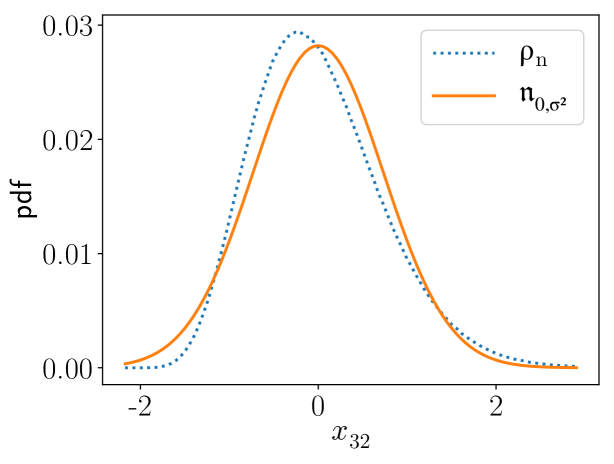
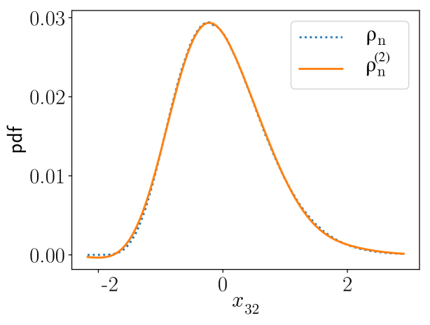
Figure 1: The probability density of sums $\frac{1}{\sqrt{n}}\sum^{n}_{i=1}f_{1}(y_{i})$ with $n=32$, $f_{1}(y)=y^{5}+y^{4}-\frac{1}{6}-\frac{1}{5}$ and $y_{i}$ generated by the tripling map from initial conditions $y_{1}$ uniformly distributed on $[0,1]$ ($\rho_{n}$, dashed line) using $10^{7}$ samples. Compared to the Gaussian distribution of the Central Limit Theorem ($\mathfrak{n}_{0,\sigma^{2}}$, left figure, solid line) and the second order Edgeworth expansion ($\rho_{n}^{(2)}$, right figure, solid line).

4 Linearly damped multi-scale systems

We now consider dynamical systems of the linear Langevin type, where the deterministic output $y_{n}$ is not simply summed, but an additional damping term is introduced as

$$x_{n+1} = \lambda x_{n}+\sqrt{\tau}y_{n}$$ (7)

$$y_{n+1} = g(y_{n})$$ (8)

where $\lambda=e^{-\tau}$, the expectation value of $y_{n}$ w.r.t. the invariant measure $\rho_{\infty}$ of $g$ is zero and we will take the limit $\tau\rightarrow 0$. These maps have been studied in [18, 3] and are a specific case of the slow-fast maps considered in [9]. As demonstrated in [9], as $\tau\rightarrow 0$, the paths of $y$ converge weakly to an Ornstein-Uhlenbeck process ${\mathrm{d}}X=-X{\mathrm{d}}t+\sigma{\mathrm{d}}W$, where $\sigma^{2}$ is the Green-Kubo variance $\sigma^{2}=\mathbbm{E}[y^{2}_{0}]+2\sum_{i=1}^{\infty}\mathbbm{E}[y_{0}y_{i}]$. Specifically, the invariant measure of $x$ converges to a Gaussian distribution. We will now study the deviations of this measure from the Gaussian distribution for small but non-zero $\tau$.

4.1 Limiting distribution

For the system (7)-(8), the dependence of $x_{n}$ on the history of the deterministic noise $y_{i}$ can be made explicit by iterating Eq. (7). We get $x_{n}=\lambda^{n}x_{0}+\sum_{i=0}^{n-1}\sqrt{\tau}\lambda^{i}y_{n-1-i}$. In the limit $n\rightarrow\infty$ the impact of the initial condition $x_{0}$ will disappear exponentially fast as $\lambda^{n}$. By a change of time $i\rightarrow i-n+1$ we are left to consider the distribution of $x_{\infty}=\sum_{i=0}^{\infty}\sqrt{\tau}\lambda^{i}y_{-i}$.

An expression for the variance of the limiting invariant measure is easily obtained, since

$$\mathbbm{E}[x^{2}_{\infty}] = \sum_{i,j=0}^{\infty}\tau\lambda^{i+j}\mathbbm{E}[y_{-i}y_{-j}]$$

$$= \sum_{i=0}^{\infty}\tau\lambda^{2i}\mathbbm{E}[y_{-i}y_{-i}]+\sum_{k=1}^{\infty}\sum_{i=0}^{\infty}\tau\lambda^{2i+k}\mathbbm{E}[y_{-i}y_{-i-k}]+\sum_{k=1}^{\infty}\sum_{i=0}^{\infty}\tau\lambda^{2i+k}\mathbbm{E}[y_{-i-k}y_{-i}]$$

$$= \tau\frac{1}{1-\lambda^{2}}\mathbbm{E}[y^{2}_{0}]+2\tau\sum_{k=1}^{\infty}\frac{\lambda^{k}}{1-\lambda^{2}}\mathbbm{E}[y_{0}y_{k}].$$

Taking the limit $\tau\rightarrow 0$, we obtain

$$\sigma^{2}_{\infty} = \lim_{\tau\rightarrow 0}\mathbbm{E}[x^{2}_{\infty}]=\frac{1}{2}\mathbbm{E}[y^{2}_{0}]+\sum_{k=1}^{\infty}\mathbbm{E}[y_{0}y_{k}].$$

4.2 Corrections to the limiting distribution

A similar calculation allows us to obtain the first Edgeworth correction term. Calculating the third cumulant of the invariant distribution, we get

$$\mathbbm{E}[x^{3}_{\infty}] = \sqrt{\tau}^{3}\sum_{i,j,k=0}^{\infty}\lambda^{i+j+k}\mathbbm{E}[y_{-i}y_{-j}y_{-k}]$$

$$= \sqrt{\tau}^{3}\mathbbm{E}[y^{3}_{0}]\frac{1}{1-\lambda^{3}}+3\sqrt{\tau}^{3}\sum_{j=1}^{\infty}\mathbbm{E}[y^{2}_{0}y_{j}]\frac{\lambda^{2j}}{1-\lambda^{3}}$$

$$+3\sqrt{\tau}^{3}\sum_{i=1}^{\infty}\mathbbm{E}[y_{0}y^{2}_{i}]\frac{\lambda^{i}}{1-\lambda^{3}}+6\sqrt{\tau}^{3}\sum_{i,j=1}^{\infty}\mathbbm{E}[y_{0}y_{i}y_{j}]\frac{\lambda^{2j+i}}{1-\lambda^{3}}$$

and in the limit $\tau\rightarrow 0$

$$c^{3,1}=\lim_{\tau\rightarrow 0}\frac{1}{\sqrt{\tau}}\mathbbm{E}[x^{3}_{\infty}] = \frac{1}{3}\mathbbm{E}[y^{3}_{0}]+\sum_{j=1}^{\infty}\mathbbm{E}[y^{2}_{0}y_{j}]+\sum_{i=1}^{\infty}\mathbbm{E}[y_{0}y^{2}_{i}]+2\sum_{i,j=1}^{\infty}\mathbbm{E}[y_{0}y_{i}y_{j}].$$ (9)

4.3 Numerical experiments

Here we consider the second order Chebyshev map $g(y)=2y^{2}-1$. For this map, we have that $\mathbbm{E}[y_{0}y_{i}]=\frac{1}{2}\delta_{0,i}$, so $\sigma^{2}_{\infty}=\frac{1}{4}$. The map is conjugate to the Bernoulli shift by $y_{0}=\cos(\pi u)=(\exp(i\pi u)-\exp(-i\pi u))/2$. Iterates are given by $y_{n}=\cos(\pi nu)$ and correlation functions are

$$\mathbbm{E}[y_{n_{1}}\ldots y_{n_{r}}]=\sum_{\sigma}\int^{1}_{0}du\prod_{j=1}^{r}\frac{1}{2}\exp(i\pi\sigma_{j}2^{n_{j}}u)=\frac{1}{2^{r}}\sum_{\sigma}\delta(\sigma_{1}2^{n_{1}}+\ldots+\sigma_{r}2^{n_{r}})$$

where the sum is over the set $\{(\sigma_{1},\ldots,\sigma_{r})|\sigma_{i}\in\{-1,1\}\}$ [2]. The only third order correlation function that is non-zero is therefore $\mathbbm{E}[y^{2}_{1}y_{2}]=\frac{1}{4}$. This shows that, by Eq. (9), $c^{(3,1)}=\frac{1}{4}$.

Figure 2 shows that the first Edgeworth approximation closely matches the deviations from Gaussianity observed in the distribution of $x_{n}$ for large $n$ and small $\tau$.

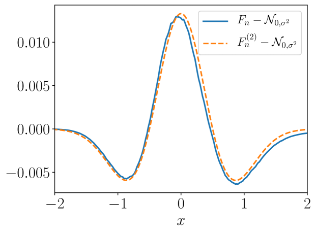
Figure 2: The difference of the cumulative distribution function (cdf) $F_{n}(x):=\mathbb{P}\{x_{n}\leq x\}$ to the limiting  Gaussian cumulative distribution function $\mathcal{N}_{0,\sigma^{2}}$ (solid line) and the difference of the cdf of the Edgeworth expansion $F_{n}^{(2)}(x):=\int_{-\infty}^{x}\rho_{n}^{(2)}(x)\,\mathrm{d}x$ to $\mathcal{N}_{0,\sigma^{2}}$ (dashed line). Here $\tau=0.01$, $n=10^{5}$ and $10^{10}$ samples are generated to estimate $F_{n}$.

5 Conclusions

In this paper we consider two applications of Edgeworth expansions.

Firstly, we have derived the Edgeworth coefficients of sums of dependent random variables. To the author’s knowledge, this is the first explicit derivation of this expansion in the literature. Equations for the expansion coefficients can be found in [10], however without derivation. Furthermore, the coefficient $c^{(4,1)}$ derived here differs substantially from the one found there. The numerical experiments in this manuscript corroborate the correctness of the expressions derived here. Furthermore, they show the high accuracy of the Edgeworth approximation. This in turn supports the hypothesis that an Edgeworth expansion holds for this dynamical system, an assumption we have not proved here.

Secondly, we show that recent results on approximations of invariant distributions of slow-fast discrete maps fit into the general framework of Edgeworth expansions. Approximations for the invariant distribution of the specific class of slow-fast linear Langeving maps have been derived in [18, 3] by different methods. The derivation given here puts these result in the context of the well-established topic of Edgeworth expansions. This provides a new view on these results and opens the way to extension to other classes of dynamical systems.

Appendix A Derivation of the Edgeworth expansion of sums

The aim is to derive expansions in orders of $\frac{1}{\sqrt{n}}$ of the cumulants of $x_{n}=\frac{1}{\sqrt{n}}\sum_{i=1}^{n}f_{1}(y_{i})$ as in Eq. (2). The expansion is most straightforwardly calculated after taking the $z$-transform w.r.t. $n$.

Taking the z-transform of the second moment $m^{(2)}_{n}:=\mathbbm{E}[x^{2}_{n}|x_{0}=0,y_{0}\sim\rho_{\infty}]$

$$\hat{m}^{(2)}(\lambda):=\sum_{n=0}^{\infty}\lambda^{n}m^{(2)}_{n} = \int\delta_{x_{0}}\otimes\rho_{\infty}({\mathrm{d}}x,{\mathrm{d}}y)\sum_{n=0}^{\infty}\lambda^{n}P^{n}x^{2}$$

$$= \int\delta_{x_{0}}\otimes\rho_{\infty}({\mathrm{d}}x,{\mathrm{d}}y)\frac{1}{1-\lambda P}x^{2}$$

where $P$ is the Koopman operator $PA(x,y)=A(x+\varepsilon f_{1}(g(y)),g(y))$ of the system

$$x_{n+1} =x_{n}+\varepsilon f_{1}(g(y_{n}))$$

$$y_{n}+1 =g(y_{n})\,.$$

Note that in this system, setting $x_{0}=0$, we have $x_{n}=\sum_{k=1}^{n}\varepsilon f_{1}(g(y))$. We will later be setting $\varepsilon=\frac{1}{\sqrt{n}}$ to obtain sums of the CLT form. The operator $P$ can be expanded as $P=\left(\sum_{k=0}^{\infty}\frac{\varepsilon^{k}}{k!}P^{k}_{x}\right)P_{y}$ with $P_{x}A(x,y)=f_{1}(g(y))\partial_{x}A(x,y)$ and $P_{y}A(x,y)=A(x,g(y))$.

Then since $(C-D)^{-1}=C^{-1}+C^{-1}DC^{-1}+C^{-1}DC^{-1}DC^{-1}+\ldots$ we have taking $C=1-\lambda P_{y}$ and $D=\lambda\left(\sum_{k=1}^{\infty}\frac{\varepsilon^{k}}{k!}P_{x}^{k}\right)P_{y}$

$$\hat{m}^{(2)}(\lambda) = \int\delta_{x_{0}}\otimes\rho_{\infty}({\mathrm{d}}x,{\mathrm{d}}y)\left(\frac{\lambda}{1-\lambda}\left(\sum_{k=1}^{\infty}\frac{\varepsilon^{k}}{k!}P_{x}^{k}\right)\frac{1}{1-\lambda}\right.$$

$$\left.+\frac{\lambda}{1-\lambda}\left(\sum_{k=1}^{\infty}\frac{\varepsilon^{k}}{k!}P_{x}^{k}\right)\frac{\lambda P_{y}}{1-\lambda P_{y}}\left(\sum_{k=1}^{\infty}\frac{\varepsilon^{k}}{k!}P_{x}^{k}\right)\frac{1}{1-\lambda}\right)x^{2}$$

other terms in the expansion are zero since they have either not enough or too many derivatives $\partial_{x}$. By the same reasoning, we can see that

$$\hat{m}^{(2)}(\lambda) = \int\rho_{\infty}({\mathrm{d}}y)\left(\frac{\lambda}{1-\lambda}\left(\frac{\varepsilon^{2}}{2!}f_{1}(g(y))^{2}\right)\frac{1}{1-\lambda}\right.$$

$$\left.+\frac{\lambda}{1-\lambda}(\varepsilon f_{1}(g(y)))\frac{\lambda P_{y}}{1-\lambda P_{y}}(\varepsilon f_{1}(g(y)))\frac{1}{1-\lambda}\right)2$$

$$= \varepsilon^{2}\frac{\lambda}{(1-\lambda)^{2}}\mathbbm{E}[f_{1}(y)^{2}]+2\varepsilon^{2}\frac{\lambda}{(1-\lambda)^{2}}\mathbbm{E}\left[f_{1}(y)\frac{\lambda P_{y}}{1-\lambda P_{y}}f_{1}(y)\right]$$

where $\mathbbm{E}[A]=\int\rho_{\infty}({\mathrm{d}}y)A(y)$ with $\rho_{\infty}$ the physical invariant measure of $y_{i+1}=g(y_{i})$. We now expand the Koopman operator as $P_{y}=p_{0}+\sum_{i=1}^{\infty}\alpha_{i}p_{i}$ , with $p_{0}=|1\rangle\langle\rho_{\infty}|$ and $p_{i}=|l_{i}\rangle\langle r_{i}|$, where the left eigenfunctions ($1$ and $l_{i}$) and right eigenfunctions ($\rho_{\infty}$ and $r_{i}$) are mutually orthogonal. We then obtain

$$\hat{m}^{(2)}(\lambda) = \varepsilon^{2}\frac{\lambda}{(1-\lambda)^{2}}\mathbbm{E}[f_{1}(y)^{2}]+2\varepsilon^{2}\frac{\lambda}{(1-\lambda)^{2}}\sum_{i=1}^{\infty}\frac{\lambda\alpha_{i}}{1-\lambda\alpha_{i}}\mathbbm{E}[f_{1}(y)|l_{i}\rangle\langle r_{i}|f_{1}(y)]$$

By the inverse z-transform (calculating the residue at $\lambda=1$ of $\hat{m}^{(2)}(\lambda)$) we have

$$m^{(2)}_{n} = \varepsilon^{2}n\mathbbm{E}[f_{1}(y)^{2}]+2\varepsilon^{2}\sum_{i=1}^{\infty}\left(n\frac{\alpha_{i}}{1-\alpha_{i}}-\frac{\alpha_{i}}{(1-\alpha_{i})^{2}}\right)\mathbbm{E}[f_{1}(y)|l_{i}\rangle\langle r_{i}|f_{1}(y)]$$

$$= \varepsilon^{2}n\mathbbm{E}[f_{1}(y)^{2}]+2\varepsilon^{2}n\mathbbm{E}\left[f_{1}(y)\frac{P_{y}}{1-P_{y}}f_{1}(y)]-2\varepsilon^{2}\mathbbm{E}[f_{1}(y)\frac{P_{y}}{(1-P_{y})^{2}}f_{1}(y)\right]$$

Noting that $\frac{P_{y}}{1-P_{y}}=\sum_{k=1}^{\infty}P_{y}^{k}$ and $\frac{P_{y}}{(1-P_{y})^{2}}=\sum_{k=1}^{\infty}kP_{y}^{k}$, by setting $\varepsilon=1/\sqrt{n}$, we have

$$c^{(2)}_{n}=m^{(2)}_{n} = \left(\mathbbm{E}[f_{1}(y)^{2}]+2\sum_{k=1}^{\infty}\mathbbm{E}[f_{1}(y)f_{1}(g^{k}(y))]\right)+\frac{1}{n}\left(-2\sum_{k=1}^{\infty}k\mathbbm{E}[f_{1}(y)f_{1}(g^{k}(y))]\right)+\mathcal{O}\left(\frac{1}{n^{2}}\right)$$

$$= \sigma^{2}+\frac{1}{n}c^{(2,1)}+\mathcal{O}\left(\frac{1}{n^{2}}\right)$$

with $\sigma^{2}$ as given in Eq. (1) and $c^{(2,1)}$ as given in Eq. (4).

Similarly, we obtain for the third moment of $x_{n}$

$$c^{(3)}_{n}=m^{(3)}_{n} = \frac{1}{\sqrt{n}}\left(\mathbbm{E}[f_{1}(y)^{3}]+\sum_{k=1}^{\infty}3\left(\mathbbm{E}[f_{1}(y)^{2}f_{1}(g^{k}(y))]+\mathbbm{E}\left[f_{1}(y)f_{1}(g^{k}(y))^{2}\right]\right)\right.$$

$$\hskip 130.08731pt\left.+6\sum_{k=1}^{\infty}\sum_{l=1}^{\infty}\mathbbm{E}[f_{1}(y)f_{1}(g^{k}(y))f_{1}(g^{k+l}(y))]\right)$$

$$= \frac{1}{\sqrt{n}}c^{(3,1)}$$

with $c^{(3,1)}$ as in Eq. (3).

For the fourth moment, we have

$$\hat{m}^{(4)}(\lambda) = \sum_{n=0}^{\infty}\lambda^{n}m^{(4)}_{n}$$

$$= \mathbbm{E}\left[\frac{\lambda}{1-\lambda}\left(f_{1}^{4}\frac{\varepsilon^{4}}{4!}\right)\frac{1}{1-\lambda}\right]4!$$

$$+\mathbbm{E}\left[\frac{\lambda}{1-\lambda}\left(f_{1}\frac{\varepsilon}{1!}\right)\frac{\lambda P_{y}}{1-\lambda P_{y}}\left(f^{3}_{1}\frac{\varepsilon^{3}}{3!}\right)\frac{1}{1-\lambda}\right]4!$$

$$+\mathbbm{E}\left[\frac{\lambda}{1-\lambda}\left(f^{3}_{1}\frac{\varepsilon^{3}}{3!}\right)\frac{\lambda P_{y}}{1-\lambda P_{y}}\left(f_{1}\frac{\varepsilon}{1!}\right)\frac{1}{1-\lambda}\right]4!$$

$$+\mathbbm{E}\left[\frac{\lambda}{1-\lambda}\left(f^{2}_{1}\frac{\varepsilon^{2}}{2!}\right)\frac{\lambda P_{y}}{1-\lambda P_{y}}\left(f^{2}_{1}\frac{\varepsilon^{2}}{2!}\right)\frac{1}{1-\lambda}\right]4!$$

$$+\mathbbm{E}\left[\frac{\lambda}{1-\lambda}\left(f_{1}\frac{\varepsilon}{1!}\right)\frac{\lambda P_{y}}{1-\lambda P_{y}}\left(f_{1}\frac{\varepsilon}{1!}\right)\frac{\lambda P_{y}}{1-\lambda P_{y}}\left(f^{2}_{1}\frac{\varepsilon^{2}}{2!}\right)\frac{1}{1-\lambda}\right]4!$$

$$+\mathbbm{E}\left[\frac{\lambda}{1-\lambda}\left(f_{1}\frac{\varepsilon}{1!}\right)\frac{\lambda P_{y}}{1-\lambda P_{y}}\left(f^{2}_{1}\frac{\varepsilon^{2}}{2!}\right)\frac{\lambda P_{y}}{1-\lambda P_{y}}\left(f_{1}\frac{\varepsilon}{1!}\right)\frac{1}{1-\lambda}\right]4!$$

$$+\mathbbm{E}\left[\frac{\lambda}{1-\lambda}\left(f^{2}_{1}\frac{\varepsilon^{2}}{2!}\right)\frac{\lambda P_{y}}{1-\lambda P_{y}}\left(f_{1}\frac{\varepsilon}{1!}\right)\frac{\lambda P_{y}}{1-\lambda P_{y}}\left(f_{1}\frac{\varepsilon}{1!}\right)\frac{1}{1-\lambda}\right]4!$$

$$+\mathbbm{E}\left[\frac{\lambda}{1-\lambda}\left(f_{1}\frac{\varepsilon}{1!}\right)\frac{\lambda P_{y}}{1-\lambda P_{y}}\left(f_{1}\frac{\varepsilon}{1!}\right)\frac{\lambda P_{y}}{1-\lambda P_{y}}\left(f_{1}\frac{\varepsilon}{1!}\right)\frac{\lambda P_{y}}{1-\lambda P_{y}}\left(f_{1}\frac{\varepsilon}{1!}\right)\frac{1}{1-\lambda}\right]4!$$

$$= \varepsilon^{4}\frac{\lambda}{(1-\lambda)^{2}}\mathbbm{E}[f_{1}^{4}]$$

$$+4\varepsilon^{4}\frac{\lambda}{(1-\lambda)^{2}}\sum_{i=1}^{\infty}\mathbbm{E}\left[f_{1}\left(\frac{\lambda\alpha_{i}}{1-\lambda\alpha_{i}}p_{i}\right)f^{3}_{1}\right]$$

$$+4\varepsilon^{4}\frac{\lambda}{(1-\lambda)^{2}}\sum_{i=1}^{\infty}\mathbbm{E}\left[f^{3}_{1}\left(\frac{\lambda\alpha_{i}}{1-\lambda\alpha_{i}}p_{i}\right)f_{1}\right]$$

$$+6\varepsilon^{4}\frac{\lambda}{(1-\lambda)^{2}}\mathbbm{E}\left[f^{2}_{1}\left(\frac{\lambda}{1-\lambda}p_{0}+\sum_{i=1}^{\infty}\frac{\lambda\alpha_{i}}{1-\lambda\alpha_{i}}p_{i}\right)f^{2}_{1}\right]$$

$$+12\varepsilon^{4}\frac{\lambda}{(1-\lambda)^{2}}\mathbbm{E}\left[f_{1}\left(\sum_{i=1}^{\infty}\frac{\lambda\alpha_{i}}{1-\lambda\alpha_{i}}p_{i}\right)f_{1}\left(\frac{\lambda}{1-\lambda}p_{0}+\sum_{j=1}^{\infty}\frac{\lambda\alpha_{j}}{1-\lambda\alpha_{j}}p_{j}\right)f^{2}_{1}\right]$$

$$+12\varepsilon^{4}\frac{\lambda}{(1-\lambda)^{2}}\mathbbm{E}\left[f_{1}\left(\sum_{i=1}^{\infty}\frac{\lambda\alpha_{i}}{1-\lambda\alpha_{i}}p_{i}\right)f^{2}_{1}\left(\sum_{j=1}^{\infty}\frac{\lambda\alpha_{j}}{1-\lambda\alpha_{j}}p_{j}\right)f_{1}\right]$$

$$+12\varepsilon^{4}\frac{\lambda}{(1-\lambda)^{2}}\mathbbm{E}\left[f^{2}_{1}\left(\frac{\lambda}{1-\lambda}p_{0}+\sum_{i=1}^{\infty}\frac{\lambda\alpha_{i}}{1-\lambda\alpha_{i}}p_{i}\right)f_{1}\left(\sum_{j=1}^{\infty}\frac{\lambda\alpha_{j}}{1-\lambda\alpha_{j}}p_{j}\right)f_{1}\right]$$

$$+24\varepsilon^{4}\frac{\lambda}{(1-\lambda)^{2}}\mathbbm{E}\left[f_{1}\left(\sum_{i=1}^{\infty}\frac{\lambda\alpha_{i}}{1-\lambda\alpha_{i}}p_{i}\right)f_{1}\left(\frac{\lambda}{1-\lambda}p_{0}+\sum_{j=1}^{\infty}\frac{\lambda\alpha_{j}}{1-\lambda\alpha_{j}}p_{j}\right)f_{1}\left(\sum_{k=1}^{\infty}\frac{\lambda\alpha_{k}}{1-\lambda\alpha_{k}}p_{k}\right)f_{1}\right]$$

$$= \varepsilon^{4}\frac{\lambda}{(1-\lambda)^{2}}\mathbbm{E}[f_{1}^{4}]$$

$$+6\varepsilon^{4}\frac{\lambda^{2}}{(1-\lambda)^{3}}\mathbbm{E}[f_{1}^{2}]^{2}$$

$$+2\varepsilon^{4}\frac{\lambda}{(1-\lambda)^{2}}\sum_{i=1}^{\infty}\frac{\lambda\alpha_{i}}{1-\lambda\alpha_{i}}(2\mathbbm{E}[f_{1}p_{i}f^{3}_{1}]+2\mathbbm{E}[f^{3}_{1}p_{i}f_{1}]+3\mathbbm{E}[f^{2}_{1}p_{i}f^{2}_{1}])$$

$$+12\varepsilon^{4}\frac{\lambda^{2}}{(1-\lambda)^{3}}\sum_{i=1}^{\infty}\frac{\lambda\alpha_{i}}{1-\lambda\alpha_{i}}(2\mathbbm{E}[f_{1}p_{i}f_{1}]\mathbbm{E}[f_{1}^{2}])$$

$$+12\varepsilon^{4}\frac{\lambda}{(1-\lambda)^{2}}\sum_{i,j=1}^{\infty}\frac{\lambda\alpha_{i}}{1-\lambda\alpha_{i}}\frac{\lambda\alpha_{j}}{1-\lambda\alpha_{j}}(\mathbbm{E}[f_{1}p_{i}f_{1}p_{j}f^{2}_{1}]+\mathbbm{E}[f_{1}p_{i}f^{2}_{1}p_{j}f_{1}]+\mathbbm{E}[f^{2}_{1}p_{i}f_{1}p_{j}f_{1}])$$

$$+24\varepsilon^{4}\frac{\lambda^{2}}{(1-\lambda)^{3}}\sum_{i,j=1}^{\infty}\frac{\lambda\alpha_{i}}{1-\lambda\alpha_{i}}\frac{\lambda\alpha_{j}}{1-\lambda\alpha_{j}}\mathbbm{E}[f_{1}p_{i}f_{1}]\mathbbm{E}[f_{1}p_{j}f_{1}]$$

$$+24\varepsilon^{4}\frac{\lambda}{(1-\lambda)^{2}}\sum_{i,j,k=1}^{\infty}\frac{\lambda\alpha_{i}}{1-\lambda\alpha_{i}}\frac{\lambda\alpha_{j}}{1-\lambda\alpha_{j}}\frac{\lambda\alpha_{k}}{1-\lambda\alpha_{k}}\mathbbm{E}[f_{1}p_{i}f_{1}p_{j}f_{1}p_{k}f_{1}]$$

By inverse z-transform of $\hat{m}^{(4)}(\lambda)$, calculating the residue of $\hat{m}^{(4)}(\lambda)\lambda^{-n-1}$ at $\lambda=1$ we obtain $m^{(4)}_{n}$. Note that there are also poles at $1/\alpha_{i}$, but these contribute terms of order $\alpha^{n}_{i}$, which decay exponentially with $n$ and therefore don’t appear in the Edgeworth expansion.

$$m^{(4)}_{n}= \varepsilon^{4}n\mathbbm{E}[f_{1}^{4}]$$

$$+6\varepsilon^{4}\frac{1}{2}(n^{2}-n)\mathbbm{E}[f_{1}^{2}]^{2}$$

$$+2\varepsilon^{4}n\sum_{i=1}^{\infty}\frac{\alpha_{i}}{1-\alpha_{i}}(2\mathbbm{E}[f_{1}p_{i}f^{3}_{1}]+2\mathbbm{E}[f^{3}_{1}p_{i}f_{1}]+3\mathbbm{E}[f^{2}_{1}p_{i}f^{2}_{1}])$$

$$+12\varepsilon^{4}\frac{1}{2}\sum_{i=1}^{\infty}\left(n^{2}\frac{\alpha_{i}}{1-\alpha_{i}}-n\left(\frac{\alpha_{i}}{1-\alpha_{i}}+2\frac{\alpha_{i}}{(1-\alpha_{i})^{2}}\right)\right)(2\mathbbm{E}[f_{1}p_{i}f_{1}]\mathbbm{E}[f_{1}^{2}])$$

$$+12\varepsilon^{4}n\sum_{i,j=1}^{\infty}\frac{\alpha_{i}}{1-\alpha_{i}}\frac{\alpha_{j}}{1-\alpha_{j}}(\mathbbm{E}[f_{1}p_{i}f_{1}p_{j}f^{2}_{1}]+\mathbbm{E}[f_{1}p_{i}f^{2}_{1}p_{j}f_{1}]+\mathbbm{E}[f^{2}_{1}p_{i}f_{1}p_{j}f_{1}])$$

$$+24\varepsilon^{4}\frac{1}{2}\sum_{i,j=1}^{\infty}\left(n^{2}\frac{\alpha_{i}}{1-\alpha_{i}}\frac{\alpha_{j}}{1-\alpha_{j}}\right.$$

$$\left.-n\left(\frac{\alpha_{i}}{1-\alpha_{i}}\frac{\alpha_{j}}{1-\alpha_{j}}+2\frac{\alpha_{i}}{(1-\alpha_{i})^{2}}\frac{\alpha_{j}}{1-\alpha_{j}}+2\frac{\alpha_{i}}{1-\alpha_{i}}\frac{\alpha_{j}}{(1-\alpha_{j})^{2}}\right)\right)\mathbbm{E}[f_{1}p_{i}f_{1}]\mathbbm{E}[f_{1}p_{j}f_{1}]$$

$$+24\varepsilon^{4}n\sum_{i,j,k=1}^{\infty}\frac{\alpha_{i}}{1-\alpha_{i}}\frac{\alpha_{j}}{1-\alpha_{j}}\frac{\alpha_{k}}{1-\alpha_{k}}\mathbbm{E}[f_{1}p_{i}f_{1}p_{j}f_{1}p_{k}f_{1}]$$

$$= \varepsilon^{4}n^{2}\left(3\mathbbm{E}[f_{1}^{2}]^{2}+12\mathbbm{E}\left[f_{1}\frac{P_{y}}{1-P_{y}}f_{1}\right]\mathbbm{E}[f_{1}^{2}]+12\mathbbm{E}\left[f_{1}\frac{P_{y}}{1-P_{y}}f_{1}\right]^{2}\right)$$

$$+\varepsilon^{4}n\left(\mathbbm{E}[f_{1}^{4}]-3\mathbbm{E}[f_{1}^{2}]^{2}+4\mathbbm{E}\left[f_{1}\frac{P_{y}}{1-P_{y}}f^{3}_{1}\right]+4\mathbbm{E}\left[f^{3}_{1}\frac{P_{y}}{1-P_{y}}f_{1}\right]+6\mathbbm{E}\left[f^{2}_{1}\frac{P_{\perp}}{1-P_{\perp}}f^{2}_{1}\right]\right.$$

$$-12\mathbbm{E}\left[f_{1}\frac{P_{y}}{1-P_{y}}f_{1}\right]\mathbbm{E}[f_{1}^{2}]-24\mathbbm{E}\left[f_{1}\frac{P_{y}}{(1-P_{y})^{2}}f_{1}\right]\mathbbm{E}[f_{1}^{2}]$$

$$+12\left(\mathbbm{E}\left[f_{1}\frac{P_{y}}{1-P_{y}}f_{1}\frac{P_{\perp}}{1-P_{\perp}}f^{2}_{1}\right]+\mathbbm{E}\left[f_{1}\frac{P_{y}}{1-P_{y}}f^{2}_{1}\frac{P_{y}}{1-P_{y}}f_{1}\right]+\mathbbm{E}\left[f^{2}_{1}\frac{P_{\perp}}{1-P_{\perp}}f_{1}\frac{P_{y}}{1-P_{y}}f_{1}\right]\right)$$

$$-12\left(\mathbbm{E}\left[f_{1}\frac{P_{y}}{1-P_{y}}f_{1}\right]\mathbbm{E}\left[f_{1}\frac{P_{y}}{1-P_{y}}f_{1}\right]+4\mathbbm{E}\left[f_{1}\frac{P_{y}}{(1-P_{y})^{2}}f_{1}\right]\mathbbm{E}\left[f_{1}\frac{P_{y}}{1-P_{y}}f_{1}\right]\right)$$

$$\left.+24\mathbbm{E}\left[f_{1}\frac{P_{y}}{1-P_{y}}f_{1}\frac{P_{\perp}}{1-P_{\perp}}f_{1}\frac{P_{y}}{1-P_{y}}f_{1}\right]\right)$$

$$= 3\varepsilon^{4}n^{2}\sigma^{4}$$

$$+\varepsilon^{4}n\left(\mathbbm{E}[f_{1}^{4}]+4\mathbbm{E}\left[f_{1}\frac{P_{y}}{1-P_{y}}f^{3}_{1}\right]+4\mathbbm{E}\left[f^{3}_{1}\frac{P_{y}}{1-P_{y}}f_{1}\right]+6\mathbbm{E}\left[f^{2}_{1}\frac{P_{\perp}}{1-P_{\perp}}f^{2}_{1}\right]\right.$$

$$+12\left(\mathbbm{E}\left[f_{1}\frac{P_{y}}{1-P_{y}}f_{1}\frac{P_{\perp}}{1-P_{\perp}}f^{2}_{1}\right]+\mathbbm{E}\left[f_{1}\frac{P_{y}}{1-P_{y}}f^{2}_{1}\frac{P_{y}}{1-P_{y}}f_{1}\right]+\mathbbm{E}\left[f^{2}_{1}\frac{P_{\perp}}{1-P_{\perp}}f_{1}\frac{P_{y}}{1-P_{y}}f_{1}\right]\right)$$

$$\left.+24\mathbbm{E}\left[f_{1}\frac{P_{y}}{1-P_{y}}f_{1}\frac{P_{\perp}}{1-P_{\perp}}f_{1}\frac{P_{y}}{1-P_{y}}f_{1}\right]-3\sigma^{4}+12\sigma^{2}c^{(2,1)}\right)$$

where $P_{\perp}=\sum_{i=1}^{\infty}p_{i}$.

Finally, setting $\varepsilon=\frac{1}{\sqrt{n}}$ and noting the $P^{k}_{\perp}=P^{k}-p_{0}$, we get for the fourth cumulant $c^{(4)}_{n}=m^{(4)}_{n}-3(m^{(2)}_{n})^{2}=m^{(4)}_{n}-3(\sigma^{2}+\frac{c^{(2,1)}}{n})^{2}=\frac{1}{n}c^{(4,1)}$ with $c^{(4,1)}$ as given in Eq. (3).

Appendix B Convergence of cumulants for the tripling map

Here we present additional evidence of the validity of the cumulant expansion of Eq. (2) for sums $x_{n}=\frac{1}{\sqrt{n}}\sum_{i=1}^{n}f_{1}(y)$ with $f_{1}(y)=y^{5}+y^{4}-\frac{1}{6}-\frac{1}{5}$ of the tripling map $y_{i+1}=3y_{i}\mod 1$.

Figure 3 demonstrates that the cumulants of $x_{n}$ indeed vary with $n$ as described in Eqs. (2). The values for $\sigma^{2}$, $c^{(2,1)}$, $c^{(3,1)}$ and $c^{(4,1)}$ analytically derived here (see Eqs. (4)-(3)) indeed give the leading order asymptotics of these cumulants. Furthermore, we show for the third and fourth cumulants that by including a higher order correction of $1/n$, the numerical values are matched extremely well. An analytic expression for this higher order correction is not derived here, but could be found be the same techniques developed here.

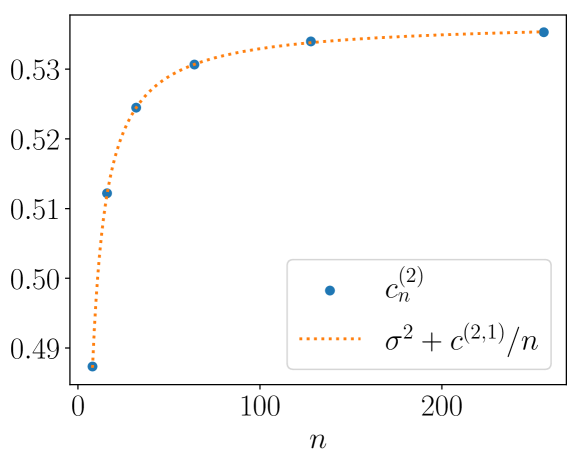
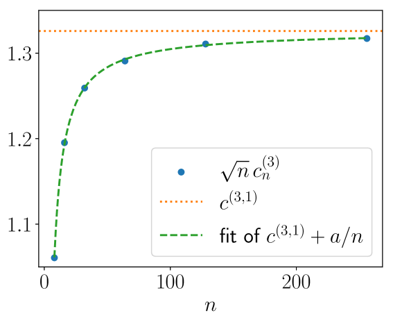
(a)	(b)
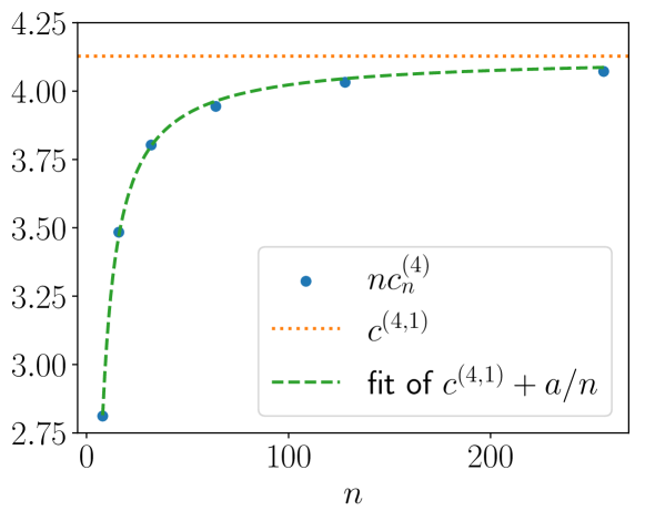
(c)

Figure 3: Cumulants of sums of the tripling map, comparing Monte Carlo simulation (blue dots) with analytic asymptotics (yellow dotted lines) and a fit of the analytic asymptotics with one higher order term (green dashed lines) for (a) the second cumulant, (b) the third cumulant and (c) the fourth cumulant.

Appendix C SageMath code to calculate tripling map cumulant expansion

Tested in SageMath version 8.6, release date 2019-01-15.

⬇

k, n, p = var(’k,n,p’)

assume(p>1)

assume(n,’real’)

assume(n>0)

# observable

A(x) = x^5 + x^4

A(x) = A(x) - integral(A,x,0,1)

# second order correlation

C(n,p) = sum(integral((A(x))*(A((p^n)*x - k)), x, k/(p^n),

(k+1)/(p^n)),k,0,(p^n) - 1)

C(n) = C(n,3)

# Green-Kubo equation

sigma2 = C(0) + 2*sum( (C(n)).expand().simplify(),

n, 1, oo, algorithm=’giac’)

# First correction to second cumulant

c21 = - 2*sum((n*C(n)).expand(),n,1,oo, algorithm=’giac’)

# third order correlations

k1, k2, n1, n2 = var(’k1,k2,n1,n2’, domain=”positive”)

C3(n1,n2) = sum(sum(integral((A(x))*(A((3^n1)*x - (k1-1)))

*(A((3^(n1+n2))*x - (3^n2)*(k1-1) - (k2-1))),

x, (k1-1)/(3^n1) + (k2-1)/(3^(n1+n2)), (k1-1)/(3^n1) + k2/(3^(n1+n2))),

k1, 1, 3^n1), k2, 1, 3^n2)

# first correction to the third cumulant

c31 = (C3(0,0) + 3*sum(C3(n1,0).expand(),n1,1,oo, algorithm=’giac’)

+ 3*sum(C3(0,n2).expand(),n2,1,oo, algorithm=’giac’)

+ 6*sum(sum(C3(n1,n2).expand(),n2,1,oo, algorithm=’giac’),

n1,1,oo, algorithm=’giac’))

# fourth order correlations

k1, k2, k3, n1, n2, n3 = var(’k1,k2,k3,n1,n2,n3’, domain=”positive”)

C4(n1,n2,n3) = sum(sum(sum(integral((A(x))*(A((3^n1)*x - (k1-1)))

*(A((3^(n1+n2))*x - (3^n2)*(k1-1) - (k2-1)))

*(A((3^(n1+n2+n3))*x - (3^(n2+n3))*(k1-1) - 3^n3*(k2-1) - (k3-1))),

x, (k1-1)/(3^n1) + (k2-1)/(3^(n1+n2)) + (k3-1)/(3^(n1+n2+n3)),

(k1-1)/(3^n1) + (k2-1)/(3^(n1+n2)) + k3/(3^(n1+n2+n3))), k1, 1, 3^n1),

k2, 1, 3^n2), k3, 1, 3^n3)

# first correction to the fourth cumulant

algo = ’sympy’

c41a = C4(n1=0,n2=0,n3=0)

c41b = sum(C4(n1=n1,n2=0,n3=0).expand(),n1,1,oo,algorithm=algo)

c41c = sum(C4(n1=0,n2=0,n3=n3).expand(),n3,1,oo,algorithm=algo)

c41d = sum((C4(n1=0,n2=n2,n3=0) - C(0)^ 2).expand(),n2,1,oo,algorithm=algo)

c41e = sum(sum((C4(n1=n1,n2=n2,n3=0) - C(n1)*C(0)).expand(),

n1,1,oo,algorithm=algo),n2,1,oo,algorithm=algo)

c41f = sum(sum((C4(n1=n1,n2=0,n3=n3)).expand(),

n1,1,oo,algorithm=algo),n3,1,oo,algorithm=algo)

c41g = sum(sum((C4(n1=0,n2=n2,n3=n3) - C(0)*C(n3)).expand(),

n3,1,oo,algorithm=algo),n2,1,oo,algorithm=algo)

c41h = sum(sum(sum((C4(n1=n1,n2=n2,n3=n3) - C(n1)*C(n3)).expand(),

n2,1,oo,algorithm=algo).expand(),n1,1,oo,algorithm=algo).expand(),

n3,1,oo,algorithm=algo)

c41 = c41a + 4*c41b + 4*c41c + 6*c41d + 12*(c41e + c41f + c41g) + 24*c41h

- 3*sigma2^2 + 6*sigma2*c21

References

• [1] Wael Bahsoun and Christopher Bose. Mixing rates and limit theorems for random intermittent maps. Nonlinearity, 29(4):1417–1433, March 2016.
• [2] Christian Beck. Higher correlation functions of chaotic dynamical systems-a graph theoretical approach. Nonlinearity, 4(4):1131, 1991.
• [3] Christian Beck. Dynamical systems of Langevin type. Physica A: Statistical Mechanics and its Applications, 233(1-2):419–440, November 1996.
• [4] Erhan Çınlar. Probability and Stochastics. Number 261 in Graduate texts in mathematics. Springer, New York ; London, 2011.
• [5] Manfred Denker. The central limit theorem for dynamical systems. Banach Center Publications, 1(23):33–62, 1989.
• [6] William Feller. An Introduction to Probability Theory and Its Applications. A Wiley publication in mathematical statistics. Wiley, New York, 2d ed edition, 1957.
• [7] Kasun Fernando and Carlangelo Liverani. Edgeworth expansions for weakly dependent random variables. arXiv:1803.07667 [math], March 2018. arXiv: 1803.07667.
• [8] G. W. Ford, M. Kac, and P. Mazur. Statistical mechanics of assemblies of coupled oscillators. J. Mathematical Phys., 6:504–515, 1965.
• [9] Georg A. Gottwald and Ian Melbourne. Homogenization for deterministic maps and multiplicative noise. Proceedings of the Royal Society A: Mathematical, Physical and Engineering Science, 469(2156), 2013.
• [10] F. Götze and C. Hipp. Asymptotic expansions for sums of weakly dependent random vectors. Zeitschrift für Wahrscheinlichkeitstheorie und Verwandte Gebiete, 64(2):211–239, June 1983.
• [11] Loïc Hervé and Françoise Pène. The Nagaev-Guivarc’h method via the Keller-Liverani theorem. Bull. Soc. Math. France, 138(3):415–489, 2010.
• [12] Ildar Abdulovich Ibragimov. Some Limit Theorems for Stationary Processes. Theory of Probability & Its Applications, 7(4):349–382, January 1962.
• [13] David Kelly and Ian Melbourne. Deterministic homogenization for fast–slow systems with chaotic noise. Journal of Functional Analysis, 272(10):4063–4102, 2017.
• [14] Stefano Luzzatto. Stochastic-Like Behaviour in Nonuniformly Expanding Maps. Handbook of Dynamical Systems, 1:265–326, January 2006.
• [15] Ian Melbourne and Andrew Stuart. A note on diffusion limits of chaotic skew-product flows. Nonlinearity, 24:1361–1367, 2011.
• [16] Matthew Nicol, Andrew Török, and Sandro Vaienti. Central limit theorems for sequential and random intermittent dynamical systems. Ergodic Theory and Dynamical Systems, 38(3):1127–1153, May 2018.
• [17] The Sage Developers. SageMath, the Sage Mathematics Software System (Version 8.6), 2019. https://www.sagemath.org.
• [18] Griffin Williams and Christian Beck. Stochastic differential equations driven by deterministic chaotic maps: analytic solutions of the Perron–Frobenius equation. Nonlinearity, 31(7):3484–3511, July 2018.
• [19] Jeroen Wouters and Georg A. Gottwald. Edgeworth expansions for slow–fast systems with finite time-scale separation. Proceedings of the Royal Society A: Mathematical, Physical and Engineering Sciences, 475(2223):20180358, March 2019.
• [20] Jeroen Wouters and Georg A. Gottwald. Stochastic model reduction for slow-fast systems with moderate time-scale separation. Multiscale Modeling and Simulation, to appear.
• [21] Lai-Sang Young. Recurrence times and rates of mixing. Israel Journal of Mathematics, 110(1):153–188, November 1999.