binoculars for Efficient, Nonmyopic Sequential Experimental Design

Abstract

Finite-horizon sequential experimental design (sed) arises naturally in many contexts, including hyperparameter tuning in machine learning among more traditional settings. Computing the optimal policy for such problems requires solving Bellman equations, which are generally intractable. Most existing work resorts to severely myopic approximations by limiting the decision horizon to only a single time-step, which can underweight exploration in favor of exploitation. We present binoculars: batch-informed nonmyopic choices, using long-horizons for adaptive, rapid sed, a general framework for deriving efficient, nonmyopic approximations to the optimal experimental policy. Our key idea is simple and surprisingly effective: we first compute a one-step optimal batch of experiments, then select a single point from this batch to evaluate. We realize binoculars for Bayesian optimization and Bayesian quadrature – two notable sed problems with radically different objectives – and demonstrate that binoculars significantly outperforms myopic alternatives in real-world scenarios.

1 Introduction

Many real-world problems can be framed as finite-horizon sequential experimental design (sed), wherein an agent adaptively designs a prespecified number of experiments seeking to maximize some data-dependent utility function. The optimal policy for sed can be formulated as dynamic programming (dp), which balances the inherent tradeoff between exploitation (immediately advancing the goal) and exploration (learning for the future). However, this optimal policy is intractable even for simple problems (Powell, 2010). Common approximation schemes include rollout, Monte Carlo tree search (Bertsekas, 2017; Powell, 2010), or simply artificially limiting the horizon, known as a myopic approximation.

In this work, we propose a novel method for efficient and nonmyopic sed, called binoculars: batch-informed nonmyopic choices, using long-horizons for adaptive, rapid sed. binoculars is inspired by the fact that the optimal batch (or non-adaptive) design is an approximation to the optimal sequential (or adaptive) design. In fact, the optimal adaptive and non-adaptive designs are exactly the same in some notable cases where the data utility does not depend on the observed outcomes, such as maximizing information gain for a fixed Gaussian process (gp) (Krause and Guestrin, 2007). Even when this is not the case, we show that the optimal batch expected utility is a lower bound of the optimal sequential expected utility. Furthermore, it is tighter than the one-step optimal policy’s implied expected utility. Motivated by this insight, binoculars iteratively computes an optimal batch of designs, then chooses one point from this batch. While many existing methods construct batch policies by simulating a sequential policy (Ginsbourger et al., 2010; Desautels et al., 2014; Jiang et al., 2018), binoculars goes the other way and “reduces” sequential design to batch design.

binoculars is a general framework applicable to any sed problem. In this paper, we realize this framework on two important yet fundamentally different sed tasks: Bayesian optimization (bo) (Kushner, 1964; Močkus, 1974; Shahriari et al., 2016) and Bayesian quadrature (bq) (Larkin, 1972; Diaconis, 1988; O’Hagan, 1991). In bo, an agent repeatedly queries an expensive function seeking its global optimum, whereas in bq the goal is to estimate an intractable integral of the function.

For both problems, many popular policies are myopic: examples include expected improvement (ei) for bo (Močkus, 1974) and uncertainty sampling (unct) for bq (Gunter et al., 2014). These are all one-step optimal for maximizing particular utility functions in expectation. While they are computationally efficient and give reasonably good empirical results, they are liable to suffer from myopia and over-exploitation. Nonmyopic alternatives have recently been applied to bo (González et al., 2016b; Lam et al., 2016; Yue and Al Kontar, 2019), and although results are promising, these are typically costly to compute.

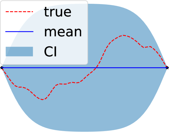
(a) initial state

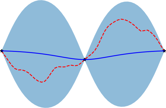
(b) ei iteration 1

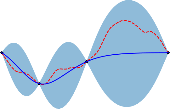
(c) ei iteration 2

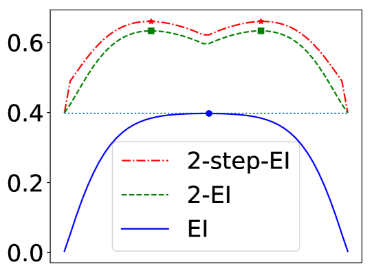
(d) ei, 2-ei and 2-step-ei

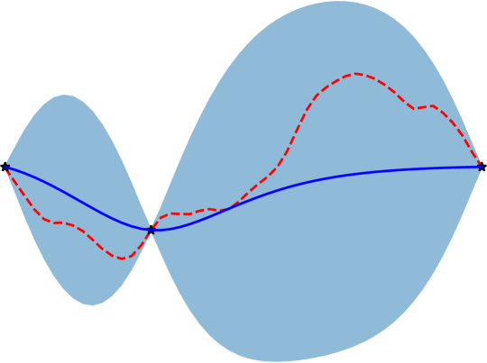
(e) 2-ei iteration 1

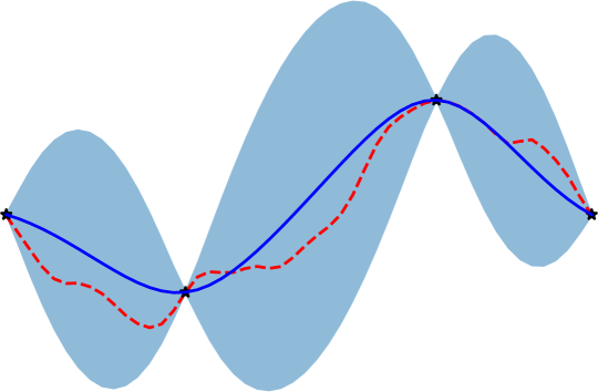
(f) 2-ei iteration 2

Figure 1: An illustration of our proposed nonmyopic method applied to bo. (a) A function in $[-1,1]$ drawn from a gp where the two end points are known to be zero. (b) and (c) show two iterations of bo with the ei acquisition function. (d) ei, 2-ei and $2$-step-ei curves with their respective maximizers. (e) and (f) show two iterations of bo where the first point is chosen from the two points maximizing 2-ei, and the second one is chosen by maximizing ei (conditioned on the observation in iteration one).

Our contributions can be summarized as follows: (1) We propose a general framework for efficient and nonmyopic sed with finite horizons, inspired by the close connection between optimal sequential and batch designs. (2) We realize the framework on two important sed problems: Bayesian optimization and Bayesian quadrature. This represents the first nonmyopic policy proposed for bq. (3) We conduct thorough experiments demonstrating that the proposed method significantly outperforms the myopic baselines and is competitive with (if not better than) state-of-the-art nonmyopic alternatives, while being much more efficient.

2 binoculars

We will first illustrate the intuition behind binoculars and provide explicit mathematical justification. We will then realize binoculars for two specific sed scenarios: bo and bq. Throughout the rest of this work, we will make extensive use of Gaussian processes (gps): a Gaussian process defines a probability distribution over functions, where the joint distribution of the function’s values at finitely many locations is multivariate normal; for more details, see (Rasmussen and Williams, 2006).

Intuition. Consider the bo example in Fig. 1, where we wish to maximize a one-dimensional objective function over an interval, conditioned on initial observations at the boundary. Suppose we are allowed to design two further function evaluations. The myopic ei policy would greedily pick the middle point first, followed by a point bisecting the left half of the domain. The resulting choices completely ignore the right half, where the maximum happens to lie.

Now consider the following alternative for designing the observations: we first construct the optimal batch of size two ($2$-ei). These points can be determined relatively efficiently as recursion is not required and reflect a better approximation of the remainder of the optimization than just looking one step ahead. We then pick any point from this batch and use ei to choose the final point given the result. This policy results in well-distributed queries and better performance. We can compare these decisions with the optimal (but expensive) policy maximizing the full lookahead expected utility ($2$-step-ei in Fig. 1(d)): our choices are nearly perfect.

2.1 The Optimal Adaptive Policy

Consider a general sed problem with a finite horizon, $T$. Let the design space be $\mathcal{X}$, response space be $\mathcal{Y}$; for $x\in\mathcal{X},y\in\mathcal{Y}$ and $\mathcal{D}\subseteq\mathcal{X}\times\mathcal{Y}$, let $p(y\mid x,\mathcal{D})$ be a probabilistic model; and let $u(\mathcal{D})$ be some utility function of observed data $\mathcal{D}$. Define $u(y\mid x,\mathcal{D})=u\bigl{(}\mathcal{D}\cup(x,y)\bigr{)}-u(\mathcal{D})$ to represent the marginal gain in utility after observing $y$ from experiment $x$ when $\mathcal{D}$ has already been observed. Let $Q_{k}(x\mid\mathcal{D})$ be the expected utility of designing experiment $x$ after observing $\mathcal{D}$ when there are $k$ steps remaining, assuming all later decisions are optimal. $Q_{k}(x\mid\mathcal{D})$ can be expressed in the form of a Bellman equation as follows:

$$Q_{k}(x\mid\mathcal{D})=\mathbb{E}_{y}[u(y\mid x,\mathcal{D})]+{}\\ \mathbb{E}_{y}\Big{[}\underset{x^{\prime}}{\textrm{max }}Q_{k-1}\big{(}x^{\prime}\mid\mathcal{D}\cup\{(x,y)\}\big{)}\Big{]},$$ (1)

where the expectation is taken with respect to $p(y\mid x,\mathcal{D})$. The optimal (expected-case) policy is

$$x^{*}=\underset{x}{\textrm{argmax }}Q_{T-i}(x\mid\mathcal{D}_{i}),$$ (2)

where $\mathcal{D}_{i}$ is the observed set at iteration $i$. The optimal policy is intractable for any moderately large horizon; in general, the complexity is $\mathcal{O}\left(|\mathcal{X}|^{T}|\mathcal{S}|^{T}\right)$, where $\mathcal{S}=\{\mathcal{D}\mid\mathcal{D}\subseteq\mathcal{X}\times\mathcal{Y}\}$, and in many settings $\mathcal{X}$ and/or $\mathcal{S}$ are uncountable. Thus, we must find some tractable approximation to proceed. A common solution is to simply limit the horizon to some manageable value $\ell$, e.g. $\ell=1$ or $2$. This is called $\ell$-step lookahead, and is computationally efficient but myopic as we severely limit our view of the future. It does not plan ahead and can thus make suboptimal tradeoffs between exploration and exploitation.

2.2 Nonmyopic Approximation via the Optimal Non-Adaptive Policy

Suppose $T$ experiments $X=\{x_{1},\dots,x_{T}\}$ must be designed simultaneously given current observations $\mathcal{D}$. The expected marginal utility of the resulting observations is

$$Q(X\mid\mathcal{D})=\mathbb{E}_{Y}[u(Y\mid X,\mathcal{D})],$$ (3)

where the expectation is taken over the joint distribution of $Y=\{y_{1},\dots,y_{T}\}$, $p(Y\mid X,\mathcal{D})$. Rewriting (3) by decomposing $X$ into $x_{j}$ and $X_{-j}$ where $X_{-j}=X\setminus\{x_{j}\}$, we have (by telescoping sum)

$$Q(X\mid\mathcal{D})=\mathbb{E}_{y_{j}}[u(y_{j}\mid x_{j},\mathcal{D})]+\\ \mathbb{E}_{y_{j}}\Big{[}Q\big{(}X_{-j}\mid\mathcal{D}\cup\{(x_{j},y_{j})\}\big{)}\Big{]}.$$ (4)

Let $X^{*}\in\textstyle{\operatorname*{arg\,max}_{X}Q(X\mid\mathcal{D})}$ be an optimal batch of experiments. For any $x^{*}_{j}\in X^{*}$, it follows that

$$\mathbb{E}_{y^{*}_{j}}\Big{[}Q\big{(}X^{*}_{-j}\mid\mathcal{D}\cup\{(x^{*}_{j},y^{*}_{j})\}\big{)}\Big{]}=\\ \underset{X_{-j}}{\textrm{max }}\mathbb{E}_{y^{*}_{j}}\Big{[}Q\big{(}X_{-j}\mid\mathcal{D}\cup\{(x^{*}_{j},y^{*}_{j})\}\big{)}\Big{]},$$ (5)

as otherwise we can construct a batch with higher utility than $Q(X^{*}\mid\mathcal{D})$. Therefore, given that the expected reward of the entire batch can be decomposed using (4), choosing any experiment $x^{*}\in X^{*}$ is equivalent to solving the following optimization: $x^{*}\in\operatorname*{arg\,max}_{x}B(x\mid\mathcal{D})$ where

$$B(x\mid\mathcal{D})=\mathbb{E}_{y}[u(y\mid x,\mathcal{D})]\\ +\underset{X^{\prime}:|X^{\prime}|=T-1}{\max}\mathbb{E}_{y}\Big{[}Q\big{(}X^{\prime}\mid\mathcal{D}\cup\{(x,y)\}\big{)}\Big{]}.$$ (6)

Comparing (6) and the Bellman equation (1), we see two differences: 1) the expectation and maximization are exchanged in the future utility term and 2) the adaptive utility is replaced by a non-adaptive counterpart. As such, (6) is clearly a lower bound of the true expected utility:

$$\underset{X^{\prime}:|X^{\prime}|=T-1}{\max} \mathbb{E}_{y}\Big{[}Q\big{(}X^{\prime}\mid\mathcal{D}\cup\{(x,y)\}\big{)}\Big{]}$$

$${}\leq{} \mathbb{E}_{y}\left[\underset{X^{\prime}:|X^{\prime}|=T-1}{\max}Q\big{(}X^{\prime}\mid\mathcal{D}\cup\{(x,y)\}\big{)}\right]$$

$${}\leq{} \mathbb{E}_{y}\left[\underset{x^{\prime}}{\textrm{max }}Q_{T-1}\big{(}x^{\prime}\mid\mathcal{D}\cup\{(x,y)\}\big{)}\right].$$ (7)

This is illustrated in Fig. 1(d): 2-step-ei corresponds to (1), and 2-ei to (6). An interesting open question is the tightness of this bound, closely related to the so-called adaptivity gap (Jiang et al., 2018; Krause and Guestrin, 2007). The similarity between these formulations provides mathematical justification for using (6) to approximate the optimal policy. Note that (6) is exactly equal to (1) if the remaining experiments become conditionally independent given the observed data, in which case there is no advantage to adaptation.

Algorithm 1 binoculars

  Input: design space $\mathcal{X}$, response space $\mathcal{Y}$, model $p(y\mid x,\mathcal{D})$, utility function $u(y\mid x,\mathcal{D})$, budget $T$

  Output: $\mathcal{D}$, a sequence of experiments and observations

  for $i\leftarrow 0$ to $T-1$ do

     Compute the optimal batch $X^{*}$ of size $T-i$

     Pick an experiment $x^{*}\in X^{*}$ and observe response $y^{*}$

     Augment $\mathcal{D}=\mathcal{D}\cup\{(x^{*},y^{*})\}$

binoculars is summarized in Algorithm 1. The primary computational cost comes from computing the optimal batch, a high-dimensional optimization problem. For the examples considered below (bo and bq), this optimization can be done using gradient-based methods and we show empirically that binoculars runs much faster than previously proposed nonmyopic methods (see section 6). Note that while we do use a batch method, it is only as a subroutine. Algorithm 1 is for sequential experimental design: in each iteration, we only observe the outcome of one experiment.

3 binoculars for Bayesian Optimization

Consider the task: $x^{*}=\textstyle{\operatorname*{arg\,max}_{x\in\mathcal{X}}f(x);}$ in this paper, we model $f$ with a gp. Suppose we have a budget of $T$ function evaluations. Once the budget has been expended, we recommend the point with the highest observed value as the maximizer of $f$. In this setting, our goal is to sequentially select a set $X=\{x_{1},x_{2},\ldots,x_{T}\}$ of $T$ points from $\mathcal{X}$ such that $\max\{y_{j}\}$ is maximized, where $y_{j}=f(x_{j})$.

Let $\mathcal{D}_{0}$ be a set of initial observations, and $y_{0}=\max_{(x,y)\in\mathcal{D}_{0}}y$ is the initial best observed value. We define the utility function as the improvement over $y_{0}$:

$$u(Y\mid X,\mathcal{D}_{0})=\left(\underset{x_{j}\in X}{\textrm{max }}y_{j}-y_{0}\right)\mathclap{{}^{+}}\textrm{ },$$ (8)

where $c^{+}=\max(c,0)$. Defining the utility as improvement allows us to write the expected utility as a Bellman equation with the same form as (1) (derivation in the appendix):

$$EI_{k}(x)=EI_{1}(x)+\mathbb{E}_{y}\left[\textstyle{\max_{x^{\prime}}}EI_{k-1}(x^{\prime}\mid x,y)\right],$$ (9)

where $EI_{k}(x)$ is the expected improvement of $k$ adaptive decisions starting from $x$, and $EI_{k-1}(x^{\prime}\mid x,y)$ is an expectation taken over the posterior belief of $f$ after further conditioning on the observation $(x,y)$ and replacing $y_{0}$ by $\max(y_{0},y)$. Observe that $\operatorname*{arg\,max}_{x}EI_{1}(x)$ exactly corresponds to the popular expected improvement (ei) policy (Močkus, 1974), which is one-step optimal; $EI_{2}(x)$ is already analytically intractable as it requires an expensive numerical integration: the integrand is $\max_{x^{\prime}}EI_{1}(x^{\prime}\mid x,y)$ and entails global optimization!

To apply binoculars, we optimize the batch ei objective, also known as $q$-ei, via the recently developed reparameterization trick and Monte Carlo approximation (Wang et al., 2016). Then we pick a point from the optimal batch; how to pick this point is discussed later. binoculars trivially extends to other utility functions such as knowledge gradient (Wu and Frazier, 2016), probability of improvement (Kushner, 1964) and predictive entropy (Shah and Ghahramani, 2015) by replacing $q$-ei appropriately.

4 binoculars for Bayesian Quadrature

Consider a non-analytic integral of the form $Z=\int f(x)\pi(x)\,\mathrm{d}{x},$ where $f(x)$ is a likelihood function and $\pi(x)$ is a prior. Such integrals frequently occur in Bayesian inference (e.g., Bayesian model selection and averaging). Bayesian quadrature operates by placing a gp on the integrand and then minimizing the posterior variance of $Z$:

$$\textstyle{\mathrm{Var}[Z\mid X]=\iint K_{X}(x,x^{\prime})\pi(x)\pi(x^{\prime})\,\mathrm{d}{x}\,\mathrm{d}{x^{\prime}},}$$ (10)

where $X=\{x_{1},x_{2},\dots,x_{T}\}$ is a set of $T$ points that needs to be optimized, and $K_{X}(x,x^{\prime})$ is the posterior covariance after conditioning on observations at $X$. If the gp hyperparameters are fixed, the optimal design $X^{*}=\textstyle{\mathrm{argmin}_{X}\mathrm{Var}[Z\mid X]}$ can be precomputed, as the posterior covariance of a gp does not depend on the observed values $f(X)$; this effectively eliminates the need for sequential experimental design in this setting.

However, in general the hyperparameters are not fixed a priori, but are instead learned iteratively in light of new observations. Furthermore, when the integrand is known to be positive (e.g., a likelihood function), it is often a good practice to place a gp on some non-linear transformation of $f$, such as $\sqrt{f}$ or $\log(f)$ (Osborne et al., 2012; Gunter et al., 2014; Chai and Garnett, 2019). As a result, the posterior gp must be approximated (e.g., by moment matching), which causes the posterior covariance to depend on the observed values. In these cases adaptive sampling becomes critical.

The adaptive version of $\mathrm{Var}[Z\mid X]$ is computationally expensive to evaluate so Gunter et al. (2014) proposed the use of uncertainty sampling (unct) (Lewis and Gale, 1994; Settles, 2010) as a surrogate, i.e. sequentially evaluating the location with the largest variance. This greedily minimizes the entropy of the integrand instead of the integral.

Formally, we use the differential entropy of the multivariate Gaussian $f(X)$ as the utility function:

$$H(Y\mid X)=\tfrac{1}{2}\log\Big{(}\det\big{(}{2\pi e\,K(X,X)}\big{)}\Big{)}.$$ (11)

Using the chain rule for differential entropy, this quantity can be expressed in the same form as (1):

$$H(Y\mid X)=H(y_{j}\mid x_{j})+\mathbb{E}_{y_{j}}[H(Y_{-j}|X_{-j},x_{j},y_{j})].$$ (12)

Note that $\textstyle{\operatorname*{arg\,max}_{x_{j}}H(y_{j}\mid x_{j})}$ corresponds to the sequential uncertainty sampling policy. To apply binoculars for bq, we must find $\textstyle{\operatorname*{arg\,max}_{X}}H(Y\mid X)$, which is the mode of a determinantal point process (dpp) (Kulesza and Taskar, 2012) defined over $q=|X|$ points. This can be done using gradient-based optimization. Note that this formulation can be applied to active learning of gps, where uncertainty sampling is also a common strategy.

Practical Considerations. Some practical issues arise when applying binoculars to real problems. First, given an optimal batch, how should one go about selecting a point from this batch? We considered several options: selecting the point with the highest expected immediate reward or randomly selecting a point, either proportional to their expected immediate reward or simply uniformly. Empirically, we found that “best” and “proportional sampling” perform similarly while “uniform sampling” is worse than the other two methods.

Second, given that binoculars is only an approximation to the optimal policy, it is not necessarily true that setting $q$ to the exact remaining budget is the best. In theory, if the model is perfect, then full lookahead is optimal. However, in practice, the model is always wrong and thus planning too far ahead could hurt the empirical performance (Yue and Al Kontar, 2019). Further, smaller values of $q$ result in more efficient computation. We empirically study the choice of $q$ in section 6.

5 Related Work

General introductions to approximate dynamic programming (dp) can be found in Bertsekas (2017); Powell (2010). On the subject of nonmyopic bo, Osborne et al. (2009) derived the optimal policy for bo, and demonstrate that it is possible to approximately compute (with great effort) the two-step lookahead policy for low-dimensional functions and that it generally performs better than the one-step policy. Ginsbourger and Le Riche (2010) also derived the optimal policy and gave an explicit example where two-step ei is better than one-step ei in expectation with a desired degree of statistical significance. González et al. (2016b) proposed a nonmyopic approximation of the optimal policy, known as glasses, by simulating future decisions using a batch bo method. Jiang et al. (2017, 2018) proposed a nonmyopic policy for (batch) active search, which can be understood as a special case of bo with cumulative reward, using a similar idea. Lam et al. (2016) proposed to use rollout for bo, which is a classic approximate dp method (Bertsekas, 2017). Yue and Al Kontar (2019) presented theoretical justification for rollout, and gave theoretical and practical guidance on how to choose the rollout horizon. Ling et al. (2016) proposed a branch-and-bound near-optimal policy for gp planning assuming that the reward function is Lipschitz continuous, and applied it to bo and active learning. Wu and Frazier (2019) proposed a gradient-based optimization of two-step ei, but each evaluation of two-step ei still requires a quadrature subroutine with an expensive integrand: optimization of one-step ei.

Of these, glasses and rollout are most related to binoculars. glasses’s acquisition function shares almost the same form as (6), except the future batch $X^{\prime}$ is constructed using a heuristic batch policy, instead of optimized with the $q$-ei objective. The batch policy adds points one by one by optimizing the sequential ei function penalized at locations already added to the batch (González et al., 2016a), and the expected utility of the chosen batch is estimated using expectation propagation.

Table 1: Average gap over 100 repeats on “hard” synthetic functions.

	Rand	EI	2.EI.b	2.EI.s	3.EI.b	3.EI.s	4.EI.b	4.EI.s	10.EI.b	10.EI.s	12.EI.s	15.EI.s
eggholder	0.498	0.613	0.614	0.633	0.604	0.657	0.646	0.694	0.622	0.704	0.738	0.694
dropwave	0.486	0.439	0.507	0.531	0.473	0.552	0.467	0.514	0.397	0.591	0.598	0.585
shubert	0.355	0.408	0.366	0.441	0.394	0.507	0.388	0.484	0.305	0.455	0.479	0.465
rastrigin4	0.374	0.801	0.769	0.775	0.817	0.821	0.840	0.805	0.797	0.804	0.793	0.799
ackley2	0.358	0.821	0.825	0.823	0.819	0.869	0.812	0.872	0.801	0.892	0.886	0.888
ackley5	0.145	0.509	0.544	0.509	0.601	0.550	0.596	0.592	0.636	0.606	0.627	0.626
bukin	0.600	0.849	0.856	0.855	0.872	0.859	0.864	0.865	0.878	0.850	0.829	0.853
shekel5	0.038	0.286	0.311	0.320	0.330	0.343	0.342	0.344	0.374	0.373	0.358	0.395
shekel7	0.045	0.268	0.346	0.313	0.349	0.325	0.352	0.370	0.399	0.358	0.412	0.386
Average	0.322	0.555	0.571	0.578	0.584	0.609	0.590	0.616	0.579	0.626	0.635	0.632

Rolling out two steps using ei as the heuristic policy is exactly equivalent to the two-step lookahead policy, up to quadrature error. Mathematically, the rollout acquisition function can also be written in a similar form as (6), except $X^{\prime}$ is adaptively constructed, depending on sampled values of $y$ instead of globally (irrespective of $y$) constructed or optimized as in glasses and binoculars. Both rollout and glasses are very expensive to compute.

While we are unaware of any existing work on nonmyopic bq, there has been some prior work on nonmyopic active learning of gps. Krause and Guestrin (2007) derived the adaptivity gap for active learning of gps under two utility functions. They also proposed a nonmyopic method for active learning of gps which separates the process into an exploration phase and an exploitation phase. They considered different acquisition functions for the exploration phase; notably, the implicit exploration (ie) method is comparable to the uncertainty sampling baseline in subsection 6.2. Hoang et al. (2014) developed a method for active learning of gps that does away with separate exploration and exploitation phases and instead naturally trades off between the two. Their proposed policy, $\varepsilon$-bal, approximates the solution to the Bellman formulation of the active gp learning problem using a truncated sampling method. They analyzed the theoretical performance of their method and also developed a pruning-based anytime version of their method.

The setting of our bq work (integration of non-negative integrands) and active learning of gps appear related yet are fundamentally different. The cited works focus exclusively on learning the hyperparameters of the gp. In our setting, the use of a transformation to model non-negativity introduces adaptivity beyond the gp hyperparameters: even if the true gp hyperparameters are known a priori, the nonlinear transformation causes the approximate gp posterior to depend on the observed values.

6 Experiments

We designed our experiments to broadly test the performance and computational cost of binoculars relative to notable myopic and nonmyopic baselines for bo and bq. We also conducted a thorough exploration of the binoculars design choices: the number of steps to look ahead and how to select a point from the optimal batch.

The primary takeaways of our experimental results are that binoculars outperforms myopic baselines while running only slightly slower and is at least as good as previously proposed nonmyopic methods while running orders of magnitude faster. This places it on the Pareto front of the running time–performance tradeoff in policy design. Furthermore, binoculars clearly demonstrates distinctively nonmyopic behavior on both bo and bq tasks, two entirely different sed problems.

We use the following nomenclature to describe binoculars: our nonmyopic bo method will be denoted as “$q$.ei.s” or “$q$.ei.b”, where $q$ is the batch size and “s” represents sampling from the batch while “b” means choosing the “best.” For bq, we replace “ei” with “dpp.” In addition to the myopic methods, ei and unct, we also compare against rollout for both tasks and glasses for bo. Each rollout method is denoted as “$q$.r.$n$”, where $q$ represents the number of steps to roll out, and $n$ is the number of samples used to estimate the expectations encountered in each step. Each glasses method is denoted as “$q$.g” where $q$ represents the size of the simulated batch. We use direct (Jones, 2009) to optimize the glasses and rollout acquisition functions, following González et al. (2016b). For all nonmyopic methods, when the remaining budget $r<q$, we set $q=r$. Thus the final decision is always made (optimally) with one-step lookahead.

For all experiments, we start with $2d$ randomly-sampled observations and perform $20d$ further iterations, where $d$ is the function’s dimensionality. Unless otherwise noted, all results presented are aggregated over 100 repeats with different random initializations. For all tabulated results, the best method is indicated in bold and the entries not significantly worse than the best (under a one-sided paired Wilcoxon signed-rank test with $\alpha=0.05$) are in blue italics.

6.1 BO Results

We implemented our nonmyopic bo policy and all baselines using BoTorch, which contains efficient ei and $q$-ei implementations. We present experiments for two rollout variants: “2.r.10” and “3.r.3.” As we will see, rolling out with horizon two is already very expensive even for just ten $y$ samples. Gauss–Hermite quadrature is used for rollout as in Lam et al. (2016). We also present experiments for two glasses variants: “2.g” and “3.g”.

We use gps with a constant mean and a Matérn $\nicefrac{{5}}{{2}}$ ard kernel to model the objective function, the default in BoTorch. We tune hyperparameters every iteration by maximizing the marginal likelihood using l-bfgs-b. We also maximize the $q$-ei acquisition function with l-bfgs-b. Complete details can be found in our attached code. We use the gap measure to evaluate the performance: gap $={(y_{i}-y_{0})}\,/\,{(y^{*}-y_{0})}$, where $y_{i}$’s are maximum observed values and $y^{*}$ is the true optimal value; we convert all problems to maximization problems by negating if necessary.

Synthetic Functions. In this section, we focus on demonstrating the superior performance of our method over ei on nine “hard” benchmark functions. These nine functions are selected by first running experiments on 31 functions with 30 repeats (see Table 4 in appendix). We then select the ones where ei terminates with average gap < 0.9. We believe nonmyopic methods are more advantageous on challenging functions; by first identifying these hard problems, we will gain more insight into the various policies. To put the bo performance into perspective, we also include a comparison against a random baseline, “Rand.”

Table 1 shows the average gap at termination. We summarize the results as follows: (1) All $q$.ei.s variants perform significantly better than ei on average, with 12.ei.s being the best and outperforming ei by a large margin. (2) The $q$.ei.s variants are consistently better than the $q$.ei.b variants (for better spacing we did not show results for 12.ei.b and 15.ei.b). (3) The performance of our method generally improves as we increase $q$, up to 12.

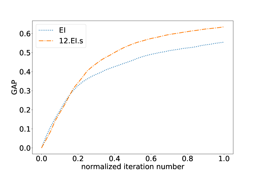
Figure 2: Average gap over nine synthetic functions demonstrating the nonmyopic behavior of 12.ei.s.

Table 2: Average gap over 50 repeats on real functions.

	EI	2.EI.s	3.EI.s	4.EI.s	6.EI.s	8.EI.s	2.G	3.G	2.R.10	3.R.3
svm	0.738	0.913	0.940	0.911	0.937	0.834	0.881	0.898	0.930	0.928
lda	0.956	1.000	0.996	0.993	0.982	0.995	1.000	0.999	0.999	1.000
LogReg	0.963	0.998	1.000	0.999	0.999	1.000	0.989	0.911	0.965	0.948
NN Boston	0.470	0.467	0.478	0.460	0.502	0.467	0.455	0.512	0.503	0.482
NN Cancer	0.665	0.627	0.654	0.686	0.700	0.686	0.806	0.755	0.708	0.698
Robot pushing 3d	0.928	0.960	0.962	0.957	0.962	0.961	0.955	0.951	0.955	0.954
Robot pushing 4d	0.730	0.726	0.695	0.695	0.736	0.697	0.765	0.786	0.770	0.745
Average	0.779	0.813	0.818	0.815	0.831	0.806	0.836	0.830	0.833	0.822

Perhaps more interestingly, we can clearly observe the nonmyopic behavior of 12.ei.s as shown in Figure 2: it is initially outperformed by the myopic ei as it explores the space. However, our method catches up to ei at $\sim$20% of the budget (on average) as it transitions to exploiting its findings until finally, it outperforms ei by a large margin. This behavior indicates that our method seamlessly navigates the exploration/exploitation tradeoff without the need for any external intervention.

Real World Functions. In this section, we compare our method against popular nonmyopic baselines: rollout and glasses. We present results on hyperparameter tuning functions used by Snoek et al. (2012); Wang and Jegelka (2017); Malkomes and Garnett (2018). These functions are evaluated on a predefined grid, so we first compute all policies (except ei) using continuous optimization, then pick the closest point from the grid.

Table 2 shows the results averaged over 50 repeats. We only show the “sampling” variants of our method; full results can be found in Table 6 First we see again all $q$.ei.s variants outperform ei by a large margin, with $q=6$ achieving the best results. Comparing 6.ei.s with the nonmyopic baselines, 2.g is the best, but the difference of 0.005 is negligible; the $p$-value under a one-sided paired signed-rank test for 6.ei.s against 2.g is $0.4257$.

We now focus on comparing the time cost of the tested methods. Figure 3 shows the average gap versus average time per iteration; the average is taken over 350 experiments (seven functions with 50 repeats each); error bars are also plotted. We again see that our methods are not significantly different from rollout and glasses in terms of gap performance, but are considerably faster in terms of average time cost per iteration (note the log scale on the time axis). Clearly, our method lies on the Pareto front in terms of computational cost and performance.

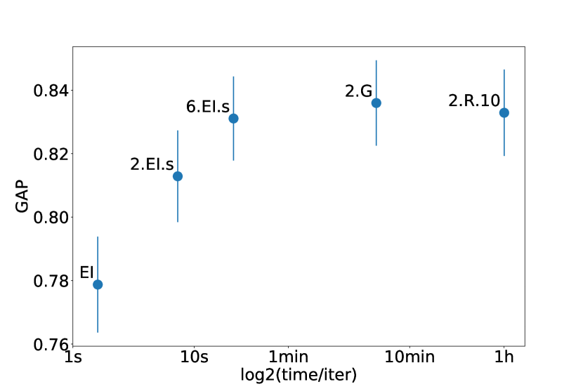
Figure 3: mean gap with error bars at termination versus time per iteration (in log scale) averaged over the seven real functions.

We also attempted to compare with the recently published practical two-step ei method (Wu and Frazier, 2019), which is intended to be a more efficient version of our 2.r.$n$. As far as we understand, the difference is first- versus zeroth-order optimization of the acquisition function. In fact, our implementation of rollout already supports gradient-based optimization thanks to automatic differentiation. However, we did not find it considerably faster than using direct. We leave it to future work to optimize the implementation and compare with our method.

It is also possible to further improve rollout’s performance using an adaptive rolling horizon in light of a recent study (Yue and Al Kontar, 2019), but it would be even more expensive to compute. In fact, Figure 1 in (Yue and Al Kontar, 2019) shows that with their adaptive horizon approach, the most frequently chosen horizon was two.

Table 3: Median fractional error values over 100 repeats on all bq functions.

	UNCT	2.DPP.b	3.DPP.b	10.DPP.b	2.DPP.s	3.DPP.s	10.DPP.s	2.R.10	3.R.3
cont	0.045	0.052	0.055	0.059	0.039	0.037	0.029	0.036	0.045
corner	0.265	0.206	0.137	0.065	0.047	0.078	0.132	0.074	0.063
discont	0.523	0.511	0.488	0.446	0.572	0.610	0.590	0.537	0.577
Gauss	0.004	0.004	0.005	0.006	0.003	0.003	0.003	0.004	0.003
mm	0.254	0.207	0.203	0.207	0.221	0.161	0.177	0.110	0.086
prod	0.007	0.007	0.007	0.007	0.007	0.006	0.006	0.012	0.012
gp	0.231	0.082	0.057	0.077	0.069	0.073	0.116	0.283	0.248
dla	0.019	0.013	0.025	0.013	0.016	0.016	0.033	0.019	0.011
Average	0.068	0.056	0.055	0.041	0.037	0.043	0.055	0.049	0.051

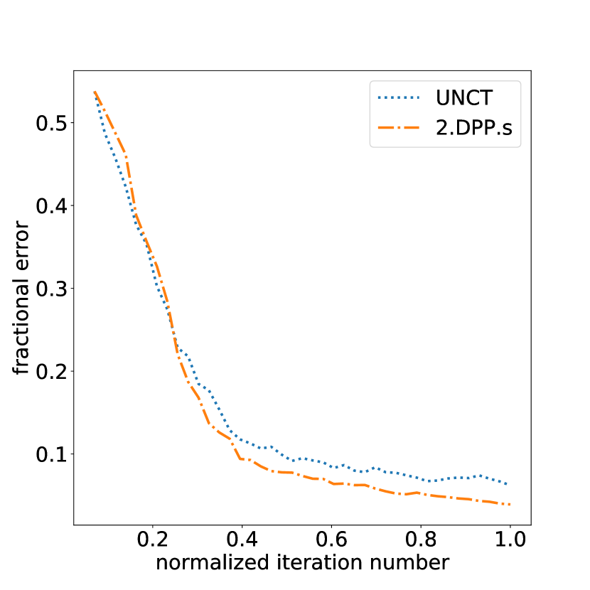
(a)

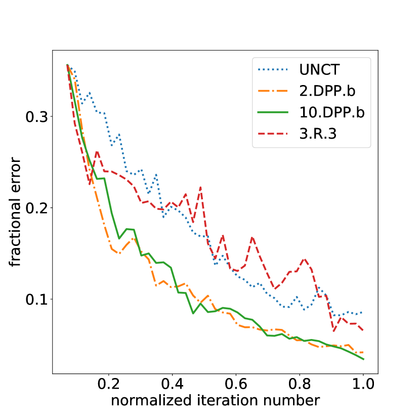
(b)

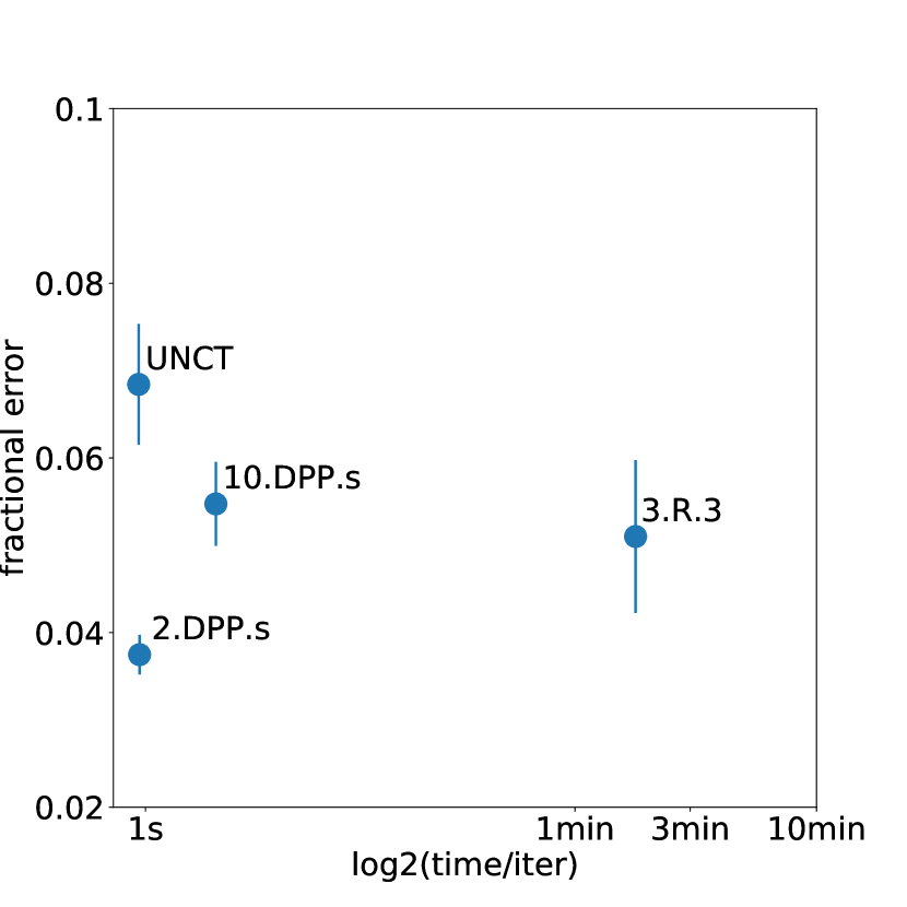
(c)

Figure 4: Median fractional error over 100 repeats against iterations or time. (a) synthetic functions, (b) real functions, (c) all functions

6.2 BQ Results

We implemented our nonmyopic bq policy and all baselines using the gpml matlab package. For all bq experiments, we use the framework of Chai and Garnett (2019): we place gp priors on the log of the integrands as they are all non-negative. We use gps with a constant mean and a Matérn $\nicefrac{{3}}{{2}}$ ard kernel to model the integrands. We tune the gp hyperparameters after each observation by maximizing the marginal likelihood using l-bfgs-b. We also use l-bfgs-b to maximize the dpp likelihood. Complete details of our implementation can be found in our attached code.

We perform experiments on five standard benchmark synthetic functions as well as one additional synthetic benchmark and two real model likelihood functions used by Chai et al. (2019). The additional synthetic benchmark is: $f(x)=\prod_{i=1}^{d}\frac{\sin(x_{i})+\nicefrac{{\cos(3x_{i}))^{2}}}{{2}}}{\nicefrac{{x_{i}^{2}}}{{4}}+0.3};$ this function was included because of its multi-modal (mm) nature. We evaluate the performance of all methods using their fractional error: $\lvert Z-\hat{Z}\rvert/{Z}$ where $\hat{Z}$ is the estimate of the integral.

Figure 4(a) indicates that 2.dpp.s exhibits the same nonmyopic behavior as 12.ei.s: it initially lags behind but eventually overtakes the myopic unct, again suggesting a superior and automatic tradeoff of exploration and exploitation.

Figure 4(c) shows the median fractional error versus average time per iteration; the average is taken over all 800 bq experiments. Our method, $2$.dpp.s, significantly outperforms all other tested methods, is considerably faster than rollout and only slightly slower than unct.

Table 3 shows the median fractional error at termination for all bq experiments. Fig. 4 shows the convergence of the fractional error as a function of both iterations and time (in $\log$ scale). These results corroborate many of the findings from our bo experiments: (1) All nonmyopic methods outperform unct on average. (2) Our proposed nonmyopic methods are competitive with, if not better than, rollout while running orders of magnitude faster.

We also note that in general, $q$.dpp.s variants tend to outperform $q$.dpp.b variants and increasing the batch size $q$ does not consistently improve the performance.

The primary conclusion here is the same as for bo: binoculars significantly and consistently outperforms myopic policies while only slightly increasing computational cost.

7 Conclusion and Future Work

We proposed binoculars: an efficient, nonmyopic approximation framework for finite-horizon sequential experimental design. binoculars computes an optimal batch, then picks a point from the batch. We gave an intuitive understanding and a mathematical justification for why this is a good approximation. We applied binoculars to Bayesian optimization and Bayesian quadrature, two entirely different problems, and empirically demonstrated that it significantly outperforms commonly used myopic policies while being much more efficient than popular nonmyopic alternatives.

As suggested by Yue and Al Kontar (2019), it would be useful to derive theories to guide the choice of lookahead horizon $q$ for our method. Another interesting theoretical question is whether we can provide explicit bounds for the adaptivity gap for a general class of problems.

Appendix A Full-Lookahead Expected Improvement as Bellman Equation

When $T=1$, i.e., there is only one evaluation left, the optimal policy degenerates to the simplest case known as expected improvement (ei):

$$x^{*}=\operatorname*{arg\,max}_{x}EI_{1}(x)\equiv\mathbb{E}[(f(x)-y_{0})^{+}].$$ (13)

Now consider $T=2$. Starting from location $x$, the improvement of the next two evaluations depends on three random variables: $y\equiv f(x)$, the next evaluation location $x^{\prime}$, and its value $y^{\prime}\equiv f(x^{\prime})$; computing the expected utility of starting from $x$ requires integrating all three variables out:

$$EI_{2}(x)=\int_{y,x^{\prime},y^{\prime}} \left(\max\{y_{1},y_{2}\}-y_{0}\right)^{+}p(y\mid x)$$

$$p (x^{\prime}\mid x,y)p(y^{\prime}\mid x^{\prime},y,x)dydx^{\prime}dy^{\prime}.$$ (14)

Given

$$\left(\max\{y,y^{\prime}\}-y_{0}\right)^{+}=(y-y_{0})^{+}+\left(y^{\prime}-\max(y_{0},y)\right)^{+}$$

[Ginsbourger et al., 2010], we have

$$EI_{2}(x) =\int_{y}(y-y_{0})^{+}dy$$

$$+\int_{y}\int_{x^{\prime}}\int_{y^{\prime}}\left(y^{\prime}-\max(y_{0},y)\right)^{+}p(y^{\prime}\mid x^{\prime},y,x)dy^{\prime}$$

$$\hphantom{+\int_{y}\int_{x^{\prime}}\int_{y^{\prime}}}p(x^{\prime}\mid x,y)dx^{\prime}p(y\mid x)dy$$

$$=EI_{1}(x)$$

$$+\int_{y}\int_{x^{\prime}}EI_{1}(x^{\prime}\mid x,y)p(x^{\prime}\mid x,y)dx^{\prime}p(y\mid x)dy$$ (15)

By Bellman’s principle of optimality, we have

$$p(x^{\prime}\mid x,y)=\textstyle{\delta(x^{\prime}-\operatorname*{arg\,max}_{x^{*}}EI_{1}(x^{*}\mid x,y))}.$$ (16)

Therefore,

$$\int_{x^{\prime}}EI_{1}(x^{\prime}\mid x,y)p(x^{\prime}\mid x,y)dx^{\prime}=\max_{x^{\prime}}EI_{1}(x^{\prime}\mid x,y),$$ (17)

and hence

$$EI_{2}(x) =EI_{1}(x)+\mathbb{E}[\max_{x^{\prime}}EI_{1}(x^{\prime}\mid x,y)].$$ (18)

In general, we have the following Bellman equation for $k$-step expected utility

$$EI_{k}(x) =EI_{1}(x)+\mathbb{E}[\max_{x^{\prime}}EI_{k-1}(x^{\prime}\mid x,y)].$$ (19)

Table 4: Average gap of 30 repeats on all 31 synthetic functions.

	EI	2.EI.b	2.EI.s	3.EI.b	3.EI.s	4.EI.b	4.EI.s	5.EI.b	5.EI.s	10.EI.b	10.EI.s
branin	1.000	1.000	0.999	1.000	0.999	1.000	1.000	1.000	1.000	1.000	0.999
rosenbrock2	0.989	0.978	0.985	0.990	0.981	0.971	0.979	0.969	0.996	0.981	0.973
rosenbrock4	0.989	0.989	0.988	0.990	0.990	0.991	0.990	0.992	0.988	0.991	0.989
rosenbrock6	0.989	0.989	0.990	0.992	0.990	0.990	0.990	0.991	0.990	0.991	0.985
hartmann3	1.000	1.000	1.000	1.000	1.000	1.000	1.000	1.000	1.000	0.999	1.000
hartmann6	0.957	0.966	0.964	0.970	0.965	0.974	0.970	0.976	0.974	0.978	0.971
eggholder	0.605	0.606	0.589	0.603	0.612	0.649	0.638	0.554	0.620	0.600	0.651
dropwave	0.455	0.489	0.524	0.475	0.599	0.538	0.550	0.435	0.613	0.448	0.651
beale	0.920	0.903	0.910	0.935	0.915	0.927	0.874	0.901	0.902	0.912	0.900
shubert	0.323	0.299	0.440	0.387	0.551	0.382	0.500	0.464	0.371	0.285	0.458
sixhumpcamel6	0.996	0.994	0.992	0.994	0.991	0.997	0.990	0.995	0.988	0.990	0.992
holder	0.936	0.873	0.913	0.941	0.930	0.965	0.949	0.950	0.948	0.883	0.936
threehumpcamel	0.988	0.981	0.978	0.970	0.978	0.981	0.949	0.975	0.931	0.971	0.930
rastrigin2	0.917	0.903	0.882	0.884	0.891	0.899	0.884	0.877	0.910	0.847	0.836
rastrigin4	0.806	0.759	0.773	0.830	0.838	0.834	0.815	0.769	0.800	0.766	0.775
ackley2	0.850	0.772	0.838	0.802	0.918	0.832	0.869	0.774	0.783	0.811	0.896
ackley5	0.528	0.557	0.555	0.579	0.562	0.602	0.594	0.604	0.620	0.671	0.621
levy2	0.925	0.949	0.927	0.933	0.915	0.960	0.961	0.958	0.913	0.963	0.929
levy3	0.960	0.948	0.962	0.954	0.962	0.951	0.961	0.960	0.968	0.969	0.951
levy4	0.968	0.959	0.970	0.970	0.974	0.962	0.950	0.976	0.976	0.970	0.972
griewank2	0.960	0.963	0.952	0.958	0.966	0.954	0.955	0.962	0.958	0.961	0.960
griewank5	0.981	0.984	0.983	0.985	0.984	0.985	0.983	0.986	0.984	0.985	0.983
stybtang2	0.999	0.970	0.999	1.000	0.999	0.999	0.999	0.999	0.992	1.000	0.999
stybtang4	0.937	0.911	0.897	0.916	0.884	0.915	0.901	0.900	0.908	0.893	0.883
powell4	0.976	0.965	0.973	0.975	0.972	0.977	0.965	0.978	0.971	0.966	0.957
dixonprice2	0.988	0.985	0.990	0.989	0.963	0.967	0.953	0.959	0.945	0.982	0.953
dixonprice4	0.987	0.986	0.985	0.958	0.981	0.982	0.986	0.982	0.985	0.987	0.971
bukin	0.822	0.864	0.865	0.844	0.860	0.851	0.861	0.852	0.850	0.885	0.826
shekel5	0.273	0.383	0.400	0.414	0.413	0.402	0.405	0.425	0.366	0.401	0.439
shekel7	0.280	0.414	0.330	0.397	0.341	0.380	0.369	0.378	0.406	0.445	0.387
michal2	0.990	0.999	0.983	0.977	1.000	1.000	0.982	0.967	0.984	1.000	0.961
Average	0.842	0.844	0.850	0.853	0.861	0.859	0.856	0.850	0.853	0.851	0.858

Table 5: Average gap of 100 repeats on all the five “hard” synthetic.

	Rand	EI	2.EI.s	3.EI.s	4.EI.s	10.EI.s	12.EI.s	2.G	3.G	2.R.10	3.R.3
eggholder	0.498	0.613	0.633	0.657	0.694	0.704	0.738	0.583	0.563	0.569	0.518
shubert	0.355	0.408	0.441	0.507	0.484	0.455	0.479	0.302	0.254	0.271	0.297
bukin	0.600	0.849	0.855	0.859	0.865	0.850	0.829	0.829	0.811	0.772	0.762
shekel5	0.038	0.286	0.320	0.343	0.344	0.373	0.358	0.265	0.175	0.378	0.350
shekel7	0.045	0.268	0.313	0.325	0.370	0.358	0.412	0.256	0.174	0.376	0.361
Average	0.307	0.485	0.512	0.538	0.551	0.548	0.563	0.447	0.395	0.473	0.458

Table 6: Average gap of 50 repeats on real functions for all $q$.ei variants.

	EI	2.EI.b	2.EI.s	3.EI.b	3.EI.s	4.EI.b	4.EI.s	6.EI.b	6.EI.s	8.EI.b	8.EI.s
svm	0.738	0.926	0.913	0.930	0.940	0.914	0.911	0.892	0.937	0.929	0.834
lda	0.956	1.000	1.000	0.998	0.996	0.996	0.993	0.999	0.982	0.995	0.995
LogReg	0.963	1.000	0.998	0.999	1.000	0.999	0.999	1.000	0.999	1.000	1.000
NN Boston	0.470	0.491	0.467	0.490	0.478	0.495	0.460	0.460	0.502	0.455	0.467
NN Cancer	0.665	0.652	0.627	0.625	0.654	0.640	0.686	0.625	0.700	0.609	0.686
Robot3d	0.928	0.959	0.960	0.944	0.962	0.956	0.957	0.960	0.962	0.967	0.961
Robot4d	0.730	0.725	0.726	0.720	0.695	0.764	0.695	0.760	0.736	0.732	0.697
Average	0.779	0.821	0.813	0.815	0.818	0.823	0.815	0.813	0.831	0.812	0.806

Appendix B Additional Bayesian Optimization Results

In the main paper, we presented bo results for nine synthetic functions. These nine functions are selected from the 31 functions shown in Table 4, with gap of ei less than 0.9. We only run up to 10.ei for all functions, so 12.ei.s and 15.ei.s are not shown. We argue that by identifying this set of “hard” functions, we are able to consistently see the advantage of nonmyopic bo methods. In Table 4, we can see all variants of our method perform better than ei on average, but other interesting patterns are weak, possibly because they are averaged out by the “easy” functions.

Table 5 includes results of rollout and glasses on five synthetic functions, after removing four from the nine for which the optima are located in the center of the domain. We remove these functions because the direct optimization procedure used in our implementations of rollout and glasses always starts evaluating exactly at the center of the domain. Thus the performance of these methods on benchmarks where the global optimum just happens to be in the center is artificially inflated. This artifact was also pointed out in Lam et al. [2016]; Wu and Frazier [2019] also excluded such results because of this.

We surprisingly see rollout and glasses perform even worse than ei on average for these five functions. This is an indicator that the synthetic benchmark functions are very different than the real-world functions. Note that Malkomes and Garnett [2018] also observed significantly different results on synthetic and real functions in their unrelated bo experiments.

Table 6 shows the average results of 50 repeats of ei and both “sampling” and “best” variants of $q$.ei on the real world functions. Different from the results on synthetic functions, we do not see “sampling” being consistently better than “best” or the other way around.

References

- Bertsekas (2017) Dimitri P. Bertsekas. Dynamic programming and optimal control, volume 1. Athena scientific, 2017. ISBN 1-886529-43-4.
- Chai and Garnett (2019) Henry Chai and Roman Garnett. Improving quadrature for constrained integrands. In Proceedings of the 22nd International Conference on Artificial Intelligence and Statistics (aistats), 2019.
- Chai et al. (2019) Henry Chai, Jean-François Ton, Michael A. Osborne, and Roman Garnett. Automated model selection with Bayesian quadrature. In Proceedings of the 36th International Conference on Machine Learning (icml), 2019.
- Desautels et al. (2014) Thomas Desautels, Andreas Krause, and Joel W Burdick. Parallelizing exploration-exploitation tradeoffs in Gaussian process bandit optimization. Journal of Machine Learning Research, 15:3873–3923, 2014.
- Diaconis (1988) Persi Diaconis. Bayesian numerical analysis. Statistical Decision Theory and Related Topics, 4(1):163–175, 1988.
- Ginsbourger and Le Riche (2010) David Ginsbourger and Rodolphe Le Riche. Towards Gaussian process-based optimization with finite time horizon. In Advances in Model-Oriented Design and Analysis (moda) 9, pages 89–96, 2010.
- Ginsbourger et al. (2010) David Ginsbourger, Rodolphe Le Riche, and Laurent Carraro. Kriging is well-suited to parallelize optimization. In Computational Intelligence in Expensive Optimization Problems, pages 131–162. 2010.
- González et al. (2016a) Javier González, Zhenwen Dai, Philipp Hennig, and Neil Lawrence. Batch Bayesian optimization via local penalization. In Proceedings of the 19th International Conference on Artificial Intelligence and Statistics (aistats), 2016a.
- González et al. (2016b) Javier González, Michael Osborne, and Neil D Lawrence. GLASSES: Relieving the myopia of Bayesian optimisation. In Proceedings of the 19th International Conference on Artificial Intelligence and Statistics (aistats), 2016b.
- Gunter et al. (2014) Tom Gunter, Michael A. Osborne, Roman Garnett, Philipp Hennig, and Stephen J. Roberts. Sampling for inference in probabilistic models with fast Bayesian quadrature. In Advances in Neural Information Processing Systems (neurips) 27, 2014.
- Hoang et al. (2014) Trong Nghia Hoang, Kian Hsiang Low, Patrick Jaillet, and Mohan Kankanhalli. Nonmyopic -Bayes-optimal active learning of Gaussian processes. In Proceedings of the 31st International Conference on Machine Learning (icml), 2014.
- Jiang et al. (2017) Shali Jiang, Gustavo Malkomes, Geoff Converse, Alyssa Shofner, Benjamin Moseley, and Roman Garnett. Efficient nonmyopic active search. In Proceedings of the 34th International Conference on Machine Learning (icml), 2017.
- Jiang et al. (2018) Shali Jiang, Gustavo Malkomes, Matthew Abbott, Benjamin Moseley, and Roman Garnett. Efficient nonmyopic batch active search. In Advances in Neural Information Processing Systems (neurips) 31, 2018.
- Jones (2009) Donald R. Jones. Direct global optimization algorithm. In Encyclopedia of optimization, pages 431–440. 2009.
- Krause and Guestrin (2007) Andreas Krause and Carlos Guestrin. Nonmyopic active learning of Gaussian processes: an exploration-exploitation approach. In Proceedings of the 24th International Conference on Machine Learning (icml), 2007.
- Kulesza and Taskar (2012) Alex Kulesza and Ben Taskar. Determinantal point processes for machine learning. Foundations and Trends in Machine Learning, 5(2–3):123–286, 2012.
- Kushner (1964) Harold Joseph Kushner. A new method of locating the maximum point of an arbitrary multipeak curve in the presence of noise. ASME. J. Basic Eng, 86(1):97–106, 1964.
- Lam et al. (2016) Remi Lam, Karen Willcox, and David H. Wolpert. Bayesian optimization with a finite budget: an approximate dynamic programming approach. In Advances in Neural Information Processing Systems (neurips) 29, 2016.
- Larkin (1972) F. M. Larkin. Gaussian measure in Hilbert space and applications in numerical analysis. Rocky Mountain Journal of Mathematics, 2(3):379–422, 1972.
- Lewis and Gale (1994) David D. Lewis and William A. Gale. A sequential algorithm for training text classifiers. In Proceedings of the 17th Annual International ACM SIGIR Conference on Research and Development in Information Retrieval, 1994.
- Ling et al. (2016) Chun Kai Ling, Kian Hsiang Low, and Patrick Jaillet. Gaussian process planning with Lipschitz continuous reward functions: towards unifying Bayesian optimization, active learning, and beyond. In Thirtieth AAAI Conference on Artificial Intelligence, 2016.
- Malkomes and Garnett (2018) Gustavo Malkomes and Roman Garnett. Automating Bayesian optimization with Bayesian optimization. In Advances in Neural Information Processing Systems (neurips) 31, 2018.
- Močkus (1974) Jonas Močkus. On Bayesian methods for seeking the extremum. In Optimization Techniques IFIP Technical Conference, pages 400–404. Springer, 1974.
- O’Hagan (1991) Anthony O’Hagan. Bayes-Hermite quadrature. Journal of Statistical Planning and Inference, 29:245–260, 1991.
- Osborne et al. (2009) Michael A Osborne, Roman Garnett, and Stephen J Roberts. Gaussian processes for global optimization. In The 3rd International Conference on Learning and Intelligent Optimization (LION3), 2009.
- Osborne et al. (2012) Michael A. Osborne, Roman Garnett, Zoubin Ghahramani, David Duvenaud, Stephen J. Roberts, and Carl E. Rasmussen. Active learning of model evidence using Bayesian quadrature. In Advances in Neural Information Processing Systems (neurips) 25, 2012.
- Powell (2010) Warren B. Powell. Approximate Dynamic Programming: Solving the Curses of Dimensionality. Wiley Series in Probability and Statistics. John Wiley & Sons, 2 edition, 2010.
- Rasmussen and Williams (2006) Carl E. Rasmussen and Christopher K. I. Williams. Gaussian Processes for Machine Learning. MIT Press, 2006.
- Settles (2010) Burr Settles. Active learning literature survey. Technical report, July 2010.
- Shah and Ghahramani (2015) Amar Shah and Zoubin Ghahramani. Parallel predictive entropy search for batch global optimization of expensive objective functions. In Advances in Neural Information Processing Systems (neurips) 28, 2015.
- Shahriari et al. (2016) Bobak Shahriari, Kevin Swersky, Ziyu Wang, Ryan P. Adams, and Nando de Freitas. Taking the human out of the loop: a review of Bayesian optimization. Proceedings of the IEEE, 104(1):148–175, Jan 2016. ISSN 0018-9219.
- Snoek et al. (2012) Jasper Snoek, Hugo Larochelle, and Ryan P Adams. Practical Bayesian optimization of machine learning algorithms. In Advances in Neural Information Processing Systems (neurips) 25, pages 2951–2959, 2012.
- Wang et al. (2016) Jialei Wang, Scott C Clark, Eric Liu, and Peter I Frazier. Parallel Bayesian global optimization of expensive functions. arXiv preprint arXiv:1602.05149, 2016.
- Wang and Jegelka (2017) Zi Wang and Stefanie Jegelka. Max-value entropy search for efficient Bayesian optimization. In International Conference on Machine Learning (ICML), 2017.
- Wu and Frazier (2016) Jian Wu and Peter Frazier. The parallel knowledge gradient method for batch Bayesian optimization. In Advances in Neural Information Processing Systems (neurips) 29, 2016.
- Wu and Frazier (2019) Jian Wu and Peter Frazier. Practical two-step lookahead Bayesian optimization. In Advances in Neural Information Processing Systems (neurips) 32, 2019.
- Yue and Al Kontar (2019) Xubo Yue and Raed Al Kontar. Why non-myopic Bayesian optimization is promising and how far should we look-ahead? A study via rollout. arXiv, 2019. Accepted to AISTATS 2020.