Random Walk Equivalence to the Compressible Baker Map and the Kaplan-Yorke Approximation to Its Information Dimension

Abstract

Simple deterministic model systems, with time-reversible equations of motion, can generate irreversible phase-space flows with attractor-repellor pairs satisfying the Second Law of Thermodynamics. Maps, and equivalent random walks, can also do this. To illustrate this paradoxical reversibility situation we study a pair of time-reversible contractive Baker Maps, $N2$ and $N3$. Both generate dissipative fractal phase-space structures. The steadily decreasing phase-space volumes exhibited by iterating these maps correspond to the dissipation associated with entropy production. Like three smooth reversible dissipative one-body phase-space flows developed in the 1980s and 1990s these simple two-dimensional maps generate fractal distributions, but in two dimensions rather than three, simplifying visualization and analyses. The continuity equation, which quantifies phase-volume loss, motivates study of the fractals’ reduced “information dimensions”, which were approximated by Kaplan and Yorke in terms of two-dimensional maps’ two Lyapunov exponents. The maps studied here generate fractal (fractional dimensional) distributions in their phase spaces. By mapping uniformly dense grids of points, fractal dimensions can be determined by “area-wise” mappings. Beginning with a uniform grid area-wise mapping of the $N2$ Baker Map provides an information dimension of 1.78969. Alternatively, as many as a trillion iterations, starting from an arbitrary point, gives a smaller “point-wise” dimensionality, $1.741_{5}$. Neither of these precisely determined estimates matches the Kaplan-Yorke conjecture value, 1.7337. In the course of studying these three different approaches to information dimension we developed random walk equivalents to both mappings, which greatly simplifies analyses. We found that for the older $N2$ Baker map the three approaches all disagree with one another! We later discovered that for the newer $N3$ Baker mapping the three approaches to information dimension, area-wise, point-wise and Kaplan-Yorke, agree.

I Numerical Simulations of ManyBody Dynamics

Statistical mechanics, developed in the 19th and early 20th centuries by Boltzmann in Austria, Gibbs in the United States, and Maxwell in England, provides a formalism giving macroscopic thermodynamic properties in terms of microscopic $(q,p)$ phase-space trajectory properties. But the complexity of systems more complicated than the ideal gas or the harmonic crystal prevented much progress on “realistic” manybody problems in particle or astrophysical dynamics. By the mid-20th century computers played a huge role in designing weapons for World War II. Their ability to solve complex problems quickly caught the attention of physicists, mathematicians, engineers, chemists, … , all of whom were stymied by the complexity of their nonlinear equations in many variables. After the war computers could be applied to many of the “hard problems” that had accumulated as fruits of the scientific revolution. Computer simulations of manybody problems were developed at universities and national laboratories worldwide. Straightforward applications of particle mechanics and statistical mechanics stimulated international collaborations long before email could make such cooperations routine.

As a result of 1980s and 1990s workshop and conference meetings in Berlin, Budapest, Gmunden, New Hampshire, Orsay, Warwick, and Zakopane, Bill, with half a dozen colleagues, developed several one-body toy-model small systems designed to shed light on the simulation of (irreversible) nonequilibrium systems with time-reversible equations of motionb1 ; b2 ; b3 ; b4 ; b5 . Among the research goals of these scientists were the resolutions of two paradoxes which had puzzled Maxwell and Boltzmann and their followers, Loschmidt’s, a consequence of time-reversible motion equations:

“How can time-reversible motion equations simulate irreversible processes?”

and Zermélo’s, a consequence of the Poincaré recurrence of any dynamical state in a bounded portion of $(q,p)$ phase space:

“How can entropy only increase if the initial state will inevitably recur?”

Applications of two computational innovations combined to provide resolutions of these paradoxes. In the mid-1980s Shuichi Nosé developed a revolutionary variant of Hamiltonian dynamicsb6 ; b7 . He introduced a control variable, his “time-scaling variable”, influencing the kinetic temperature. This modified dynamics, still time-reversible, enabled the simulation of systems at a specified kinetic temperature rather than constant energy. This work was improved and simplified by Bill Hooverb8 ; b9 as a result of conversations he and Nosé had near the Notre Dame Cathedral in 1984. They had met by chance at a train station in Paris, a few days prior to a CECAM workshop in Orsay. By 1986 Nosé-Hoover dynamics was generalized to the simulation of nonequilibrium steady states. Bill, along with half a dozen colleagues, developed three toy-model problems illustrating applications of the new mechanics’ temperature control to three nonequilibrium systems: the Galton Boardb2 , the Galton Staircaseb1 ; b3 , and, a decade later, the Conducting Oscillatorb5 . The three problem types all exhibited irreversible chaotic solutions (exponentially sensitive to perturbations) despite the deterministic time-reversibility of the dynamics. [ 1 ] The Galton Board problem follows the field-driven isokinetic motion of a hard disk through a fixed lattice of identical hard-disk scatterers. The resulting phase-space distribution is fractalb2 ; b10 , a distribution with a nonintegral topological dimensionality. [ 2 ] The Galton Staircase problem likewise follows a thermostatted field-driven motion, but of a mass point with momentum $p$in a sinusoidal potential. The equations of motion for the Galton Staircase are

$$\dot{q}=p\ ;\ \dot{p}=F-\sin(q)-\zeta p\ ;\ \dot{\zeta}=p^{2}-T\ .$$

[ 3 ] The Conducting Oscillator problemb5 simulates the motion of a heat-conducting harmonic oscillator thermostatted with a coordinate-dependent temperature $T(q)=1+\epsilon\tanh(q)$.

All three of these Nosé-Hoover modifications of Hamiltonian flows can generate fractal distributions and do also obey the phase-space continuity equation expressing the comoving conservation of probability $fdqdpd\zeta=f\otimes$. Here $f$ is the probability density and $\otimes$ is an infinitesimal phase volume element:

$$(\dot{f}/f)=-(\dot{\otimes}/\otimes)=-[(\partial\dot{q}/\partial q)+(\partial\dot{p}/\partial p)+(\partial\dot{\zeta}/\partial\zeta)]=\zeta=(\dot{S}/k)\ .$$

Gibbs’ and Boltzmann’s identification of entropy with $\langle-k\ln f\rangle$ identifies the Nosé-Hoover friction coefficient $\zeta$ with entropy production. This is a useful result in interpreting nonequilibrium simulations including the instantaneous heat transfer to the external heat baths represented by the temp0erature-control variable $\zeta=(\dot{S}/k)$. Here $k$ is Boltzmann’s constant. For convenience we usually choose it equal to unity.

In these three deterministic time-reversible models thermostatting is implemented by integral feedback forces imposing a given kinetic temperature $\langle\ p^{2}\ \rangle$, with control forces $\{-\zeta p\}$ linear in the moving particle’s momentum $p$. These model systems are sufficiently simple that their phase-space distributions can be analyzed preciselyb10 ; b11 to determine the power-law variation of phase-space bin probabilities P($\delta$) with bin size $\delta$. The resulting box-counting and correlation dimensionalities of the fractal distributions describe the scaling of the zeroth and second powers of bin probabilities $\{$ P $\}$. The information dimension is logarithmic. It corresponds to $\langle\ln$(P)$\rangle/\ln(\delta)$, giving the powerlaw variation of the density of points with respect to the bin size. Information dimension arises naturally in analyzing thermostatted mechanics and is the focus of our attention here. Because one-, two-, and three-dimensional objects in a three-dimensional space have probabilities varying as the first, second, and third powers of the bin size $\delta$ the definition of the information dimension, $D_{I}=\langle\ln({\rm P})\rangle/\ln(\delta)$, is a natural generalization of dimension from the integers 1, 2, 3 to a continuously variable “fractal” value. In the special toy-model cases studied in the 1980s and 1990s most distributions turned out to have fractional rather than integral dimensionalities, characteristic of nonequilibrium steady states. Under some conditions one-dimensional dissipative limit cycles resultedb5 .

II Time-Reversible Chaos and the Two-Dimensional Baker Map

Solutions of Hamilton’s or Lagrange’s or Newton’s or Nosé-Hoover’s motion equations are all “time-reversible”. A transparent example is the solution of the one-dimensional harmonic oscillator with unit mass and force constant;

$$\dot{q}=p\ ;\ \dot{p}=-q\rightarrow\ddot{q}=-q\ [\ {\rm Hamiltonian\ Oscillator}\ ]\ ;$$

$$\ddot{x}=-x(t)\ [\ {\rm Newtonian\ Oscillator}\ ]\ ;$$

$$\ddot{x}=-x(t)-\zeta\dot{x}\ ;\ \dot{\zeta}=\dot{x}^{2}-T\ [\ {\rm Nos\acute{e}-Hoover\ Oscillator}\ ]\ .$$

Given initial values of the coordinate, $x$ or $q$, at the current and previous times, $x(t)$ and $x(t-dt)$, one can integrate either forward or backward, extending the coordinates’ time series as far into the future or past as desired. Time reversibility can be confirmed by integrating for one timestep, changing the sign of $dt$ and integrating (backward in time) for one step, and then again changing the time, returning to the initial values of $x(t),\dot{x}(t),\zeta(t)$ or $(q(t),p(t))$. Adding a Nosé-Hoover thermostatting force $-\zeta p$ the dynamics retains time-reversibility so long as $\zeta$ changes sign in the reversed motion, behaving like a momentum variableb9 .

Studies of chaotic flows require at least three dynamical variables. In a bounded region of one-or-two-dimensional space a deterministic trajectory must either stop or trace out a periodic orbit, and so cannot be chaotic. The graphics can be simplified by considering projections or cross-sections of three-dimensional flows. A little reflection shows that cross-sections of flows are equivalent to maps, with deterministic finite jumps from one phase-space point to another rather than a smooth continuous flow. Let us consider the reversibility of maps. Textbook maps were typically both dissipative and irreversible in 1987b1 . At that time Bill had no idea that maps could be time-reversible. He wroteb1 :

“The mathematical structures of dissipative maps and the hydrodynamic equations are inherently irreversible. The Nosé-Newton equations are different: They are time-reversible.”

III Generating Time-Reversible Baker Maps

Figure 1: The two-panel $B(x,y)$ (at left) and $N2(q,p)$ (at right) versions of the compressible nonequilibrium Baker Map. For convenience the mapping is illustrated in the unit square, $0<x,y<1$ at left and in a $2\times 2$ diamond at the right with $-\sqrt{2}<q,p<+\sqrt{2}$. In both cases the mapping $T$, not to be confused with temperature, changes the sign of the vertical coordinate, $T(\pm x,\pm y)=(\pm x,\mp y)$ at the left and $T(\pm q,\pm p)=(\pm q,\mp p)$ at the right. Note that the bottom leftmost configuration differs from a time-reversed image of the top left image, showing that map $B$ is not time-reversible. The 45 degree rotated mapping $N2$ at the right satisfies time reversibility $N2TN2T(q,p)=I(q,p)=(q,p)$, and so is a more faithful analog of time-reversible classical mechanics. Here $I$ is the identity mapping.

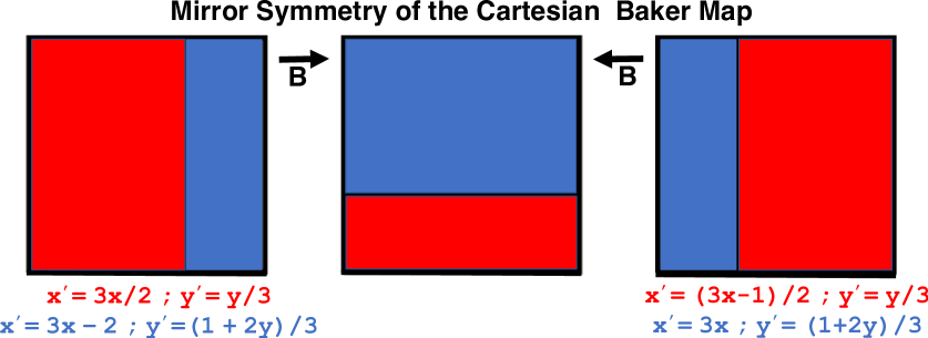
Figure 2: The mirror symmetry of the Baker map implies that the dividing line between the two mappings, contracting the red region and expanding the blue, can be located at $x=1/3$ (at the right, above) or $x=2/3$ (at the left). The analytic forms of the red and blue mappings are colored accordingly. The red mappings halve the area while the blue mapping expand, in both cases by a factor of two. The primed coordinates describe coordinates in the central unit square.

Figure 3: 100,000 iterations of the inverse $N2^{-1}$ of the nonequilibrium Baker Map $N2(q,p)$ generate the fractal repellor (red, at the left). Changing the sign of the vertical “momentum” $p$ generates the fractal attractor (blue, at the right) from the repellor. Point-wise analyses of either fractal with trillions of iterations suggest an information dimension $D_{I}=1.741_{5}$. The mappings shown here were achieved “pointwise”, by repeated mappings of a single point. The limiting extrapolated steady-state information dimensions of the two fractals, based on large-$n$ meshes of width $(1/3)^{n}$, are close to 1.741, as is discussed in the text. The Kaplan-Yorke Lyapunov dimension is significantly smaller, 1.7337 for the two rotated Baker maps. For a related puzzle see Figure 3.

If a time-reversible map $M(q,p)$ maps a coordinate $q$ and momentum $p$ forward for one step then it must obey the identity $I=MTMT$, where $T$ changes the sign of the momentum $p$ and $I$ is the identity,

$$I(q,p)=(q,p)\ ;\ M(q,p)=(q^{\prime},p^{\prime})\ ;\ T(q,\pm p)=(q,\mp p)\ .$$

We choose the left-to-right convention, 123…, for the ordering of sequences of mappings. For instance, with M time-reversible, the sequence of four mappings $MTMT$ corresponds first to stepping forward with $M$, second to shifting to reverse, third to stepping backward with $M$, and fourth, changing the direction of motion from reverse to forward, matching the original direction of motion, $MTMT=I$.

Reversibility can be implemented by considering the rotational modification $N2$ of the Baker’s Map $B$, shown at the right in Figure 1. This modification clears the way for area changes corresponding to the production of Boltzmann-Gibbs’ entropy. The two-panel Baker map $N2$ (at the right) doubles the size of an area element $dxdy$ in the red region at upper left and halves that of an element from the larger blue region. The two mappings (one for red points and one for blue) are linear, with the “new” coordinate or momentum of the form $A+Bq+Cp$. The constants $(A,B,C)$ can be identified relatively easily from the mappings of the vertices of like-colored regions. See the example equations in Figure 2.

The resulting mappings for the two-panel Baker maps can be expressed as follows: In conventional Cartesian coordinates, with $0<x,y<1$ the Cartesian map $B$ for red elements of area in the top row Figure 1 is

$$x<(1/3)\longrightarrow x^{\prime}=3x\ ;\ y^{\prime}=(1+2y)/3\ [\ {\rm Red\ Mapping}\ ]\ .$$

Blue elements likewise follow a linear mapping:

$$x>(1/3)\longrightarrow x^{\prime}=(3x-1)/2\ ;\ y^{\prime}=y/3\ [\ {\rm Blue\ Mapping}\ ]\ .$$

To check the reversibility of these maps simply apply the combination $BTBT$ to the vertices and check to see whether or not the original points are recovered. Because the combination mapping $BTB$ produces four parallel horizontal strips rather than two vertical strips at the lower left of Figure 1 the Cartesian Baker Map $B$ (at top left) is not time-reversible.

By analogy with flows a map $M$ is said to be time-reversible when it can be reversed by a three-step process: [ 1 ] changing the signs of the momentum-like variables, [ 2 ] propagating all the variables one (“backward”) iteration, and then changing the signs of the momenta once more, so that the inverse of the map $M$ is given by $M^{-1}=TMT$. In ordinary Hamiltonian mechanics the $T$ mapping simply maps $(\pm q,\pm p)\rightarrow(\pm q,\mp p)$. Bill’s conversations with Bill Vance and Joel Keizer during Vance’s graduate work at the University of California’s Davis campus led us to a nonequilibrium rotated version of the Baker Map $B$ which we call $N2$, for “Nonequilibrium”with two panels. This Map’s domain is the diamond-shaped region, centered on $(q,p)=(0,0)$ and shown at the right of Figure 1 and again in Figure 3. Now imagine that the map $N2$ is applied to a representative input point $(q,p)$. This operation produces the next point $(q^{\prime},p^{\prime})$.

Our rotated nonequilibrium Map, $N2(q,p)\rightarrow(q^{\prime},p^{\prime})$ has the following analytic form : For (red) twofold expansion, $q<p-\sqrt{2/9}$ :

$$q^{\prime}=(11q/6)-(7p/6)+\sqrt{49/18}\ ;\ p^{\prime}=(11p/6)-(7q/6)-\sqrt{25/18}\ .$$

For (blue) twofold contraction, $q>p-\sqrt{2/9}$ :

$$q^{\prime}=(11q/12)-(7p/12)+\sqrt{49/72}\ ;\ p^{\prime}=(11p/12)-(7q/12)-\sqrt{1/72}\ .$$

Figure 3 shows the resulting concentration of probability into bands parallel to the attractor’s bottom left and the repellor’s upper left edges of their diamond-shaped domains.

Although the algebra is more cumbersome we have chosen to use the rotated $N2(q,p)$ version of this map, centered on the origin and confined to a diamond-shaped region of sidelength 2, as shown at the right in the Figures. We regard the horizontal $q$ variable as a coordinate and the vertical $p$ variable as a momentum. Figures 1 and 3 illustrate the time-reversibility of the $(q,p)$ map. This similarity to nonequilibrium molecular dynamics, along with the square roots generating the $45^{o}$ rotation, are twin advantages of this nonequilibrium diamond-shaped map $N2$. The square roots eliminate most of the artificial periodic orbits resulting from finite computer precision. Beginning at the center point of the Cartesian rational-number square map, $(x,y)=(0.5,0.5)$, leads to a periodic orbit of just 3095 single-precision iterations. Starting instead at the equivalent central point of the irrational-numbered diamond map, $(q,p)=(0.0,0.0)$, leads to a single-precision periodic orbit of 1,124,068 iterations. With double-precision arithmetic the orbits are much longer. $10^{12}$ such $(x,y)$ iterations from the same initial condition gave no repeated points. Let us next consider an approximate theoretical approach to analyzing the Baker fractal followed by two computational approaches. We will find several interesting surprises in so doing.

IV Kaplan and Yorke’s Conjectured Dimension

It has been arguedb11 that the fractal information dimension is best suited to characterizing fractal distributions of points because it is uniquely insensitive to changes of variables. For that reason Kaplan and Yorke’s conjectured relation between the Lyapunov spectrum and the information dimension, $D_{KY}=1-(\lambda_{1}/\lambda_{2})\stackrel{{\scriptstyle?}}{{=}}D_{I}$ in this case, is of special interest. Because the Baker Map is linear one might expect that it would likely follow the conjectured relation. Kaplan and Yorke suggested that a linear interpolation formula between the number of terms in the last positive sum of exponents, starting with the largest, $\lambda_{1}$, and the number of terms in the next sum ( the first negative sum, one greater than the number of terms in the previous sum), would be a useful estimate for the information dimensionb12 . In fact they cite many a case, including theoretical work carried out by L. S. Young, for which their conjectured estimate is exactly correct.

The blue portion of the compressible Baker Map of $B$ in Figure 1 represents the (2/3) of the measure that stretches horizontally by a factor (3/2) while the red portion represents that (1/3) of the measure that stretches by a factor of 3 in the same direction, horizontally. As a result the longtime stretching rate per iteration is

$$\lambda_{1}=(2/3)\ln(3/2)+(1/3)\ln(3)=(1/3)\ln(27/4)=0.63651\ .$$

Likewise (2/3) of the measure shrinks vertically by a factor 3 as does (1/3) by a factor (2/3) so that

$$\lambda_{2}=(2/3)\ln(1/3)+(1/3)\ln(2/3)=(1/3)\ln(2/27)=-0.86756\ .$$

The linear interpolation between the single-term “positive sum”, 0.63651, and the two-term sum, $0.63651-0.86756=-0.23105$, gives an interpolated “number of terms for a sum of zero”, 1 + ($0.63651/0.86756)=1.73368$. This dimension, sometimes called the “Lyapunov dimension” is the Kaplan-Yorke dimension $D_{KY}$.

In their 1998 paperb4 , presented at the 1997 Budapest Meeting on Chaos and Irreversibilityb16 , Bill and Harald Posch introduced the two-panel nonequilibrium $N2$ Baker map. The model stimulated more work at the meetingb17 and subsequentlyb18 . In 2005 Kumĉák wrote a very readable paperb19 emphasizing the connection of “Generalied Baker maps” to the phase-space contractability (to fractals) providing improved understanding of the emergence of the Second Law of Thermodynamics for such models. Kumiĉák characterized his generalized maps with the variable $w$. The fraction of a mapping occupied by the narrowest strip, is $1/w$, 1/3 for the $N2$ mapping of Figures 1 and 2. Like Hoover and Posch, he assumed that Kaplan and Yorke’s conjecture for the information dimension was true. For the nonequilibrium $w$ values of 3, 4, and 5 he quotes information dimensions 1.734, 1.506, and 1.376, as well as a general formula for the generalized Baker Maps. A decade later, with Florian Grondb13 , we checked this assumption for a flow, as opposed to a map. We chose a four-dimensional chaotic flow,

$$\{\ \ddot{q}=-q-\zeta\dot{q}-\xi\dot{q}^{3}\ ;\ \dot{\zeta}=\dot{q}^{2}-T\ ;\ \dot{\xi}=\dot{q}^{4}-3\dot{q}^{2}T\ \},\longrightarrow D_{KY}=2.80>D_{I}=2.56\ .$$

and soon discovered that the conjecture fails in that case. For that four-dimensional chaotic problem, with a relatively strong temperature gradient, $T=1+\tanh(q)$, the interpolated Lyapunov sum, between those for two and for three exponents, $\lambda_{1}+\lambda_{2}+0.80\lambda_{3}$ , vanishes. The consequent Kaplan-Yorke dimension, 2.80, differs by about ten percent from the bin-based dimensionality of 2.56. Those results, along with those that follow here leave the status of the conjecture perplexing. It would be useful to have a clear informal description of maps for which the conjecture is known to be true accompanied by an illustrative list of situations where it fails.

V Area-Wise and Point-Wise Information Dimensions

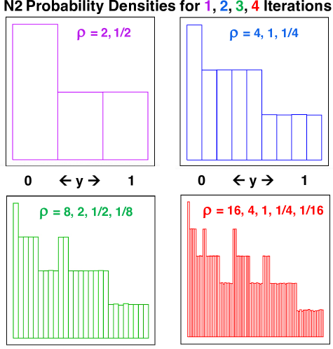
Figure 4: Histograms of the (base-4 logarithm of) probability density $\rho(y)$ for 1, 2, 3, and 4 area-wise iterations of the $y$ component of the Baker Map $B$. Notice that the number of bins at each level of probability is the product of a binomial coefficient and a power of two, in the red case $1\times 1$, $4\times 2$, $6\times 4$, $4\times 8$, $1\times 16$. Notice here that the leftmost third of the interval, with summed-up probability 2/3, is reproduced as a scale model (with the same information dimensionality) in the rightmost two thirds of the interval, with probability 1/3. The information dimensions of all these iterates, $D_{I}=\sum(P\ln P)/\ln(\delta)=0.78969$ are identical. This scale-model result differs from both the Kaplan-Yorke value of 0.7337 and the extrapolated 0.741 based on mesh sizes of $(1/3)^{n}$ and illustrated in Figure 4. The histograms were constructed by binning (in 3, 9, 27, and 81 bins) the results of 1, 2, 3, and 4 iterations of 100,000 equally spaced initial values on the interval $0<y<1$.

Analyzing the fractal structures generated by the compressible $N2$ Baker Map reveals that there is no fractal structure in the $x$ direction. See again the rotated maps’ fractals in Figure 3. Only the $y$ coordinate reveals a fractal. This suggests two computational approaches to determining the information dimension associated with the $y$ direction in map $B$ or the $q=p$ direction in map $N2$: [ 1 ] Propagating a series of area mappings, starting with a homogeneous square-lattice covering of the initial unit square or the rotated $2\times 2$ diamond-shaped domain of Figure 1; [ 2 ] Accumulating a time series of bin occupancies of points, with as many as trillions of iterations generating a long sequence of points started at an arbitrary initial point. Approaches [1] and [2], area-wise and point-wise, respectively appear to be equally legitimate routes to information dimension. It was a surprise to find that the two don’t agree although both these approaches do reach well-defined limits. Another approach, [3], which we term “stochastic”, adopts random numbers for successive values of $x$ rather than using the more time-consuming analytic $N$ mapping. With random numbers $\{0<r<1\}$ the third approach is simply a confined random walk $(0<y<1)$ with red-region “up” steps one-third of the time and “down” steps two-thirds of the time. The programming of a single stochastic step requires two calls to a random-number generator (for which we use a standard random-number FORTRAN subroutine). Note the underscore in the “calls” below:

call random_number(r)
if(r.lt.1/3) y = (1+2y)/3
if(r.gt.1/3) y = (0+ y)/3
call random_number(x) for two-dimensional grid

We have already seen, in Figure 4, that the area-wise mapping used to generate the histograms, simply repeats the single-iteration three-bin information dimension, 0.78969. The point-wise mapping is simpler. It is only limited by available computer time. A personal computer is quite capable of trillions of point-wise iterations. A billion point-wise iteration take about a minute of computer time. Using double-precision and an initial point $(x,y)=(0.5,0.5)\leftrightarrow(q,p)=(0,0)$ the two algorithms, pointwise and stochastic agree, as expected, to four-figure accuracy, with the following three-strip populations with a total of one billion points and the resulting entropies:

$${\rm pointwise}:666\ 681\ 049+295\ 151\ 739+38\ 167\ 212\rightarrow D=0.6873;$$

$${\rm stochastic}:666\ 631\ 518+295\ 178\ 423+38\ 190\ 059\rightarrow D=0.6874.$$

The close agreement shows that area-wise mapping is an outlier and suggests the adoption of point-wise distributions. We consider some interesting details of that approach next.

VI Point-Wise Information Dimension From The Baker Map Using a Random-Walk Algorithm

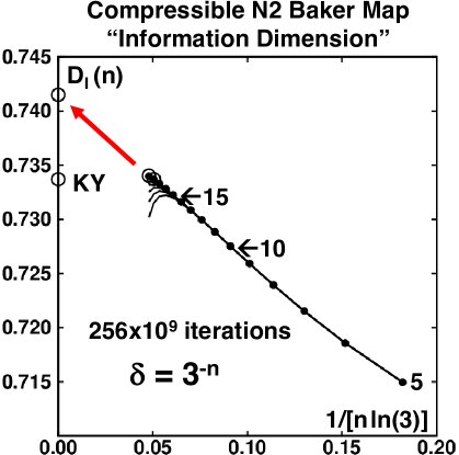
Figure 5: Stationary estimates of $D_{I}$ for the confined-random-walk model of the Baker Map with results for $3^{5,10,15}$ equal bins emphasized. We saw above that the two values shown at the zero bin-size limit ($\delta\to 0$) are the Kaplan-Yorke dimension, 0.7337, and a plausible extrapolation of trillion-iteration computations with as many as $3^{19}$ bins, $0.741_{5}$. Note the qualitative difference of the mesh dependence here ( the slope is uniformly negative here ) compared to those shown for four other sets of bin sizes, $4^{-n},\ 5^{-n},\ 6^{-n},\ 7^{-n}$ in Figures 6 and 7. The two open circles at $n=18$ and 19 correspond to $1.024\times 10^{12}$ iterations. The smaller dots correspond to sequences of 256 billion points.

It is easy to verify that the one-dimensional and two-dimensional point-wise mappings agree with one another for readily convergent simulations with $\delta=3^{-10}$ or $3^{-15}$. Such results agree very well with the stochastic map where ${\cal R}$ represents a random number from the interval $(0<x<1)$.

$${\cal R}<(1/3)\rightarrow y^{\prime}=(1+2y)/3\ ;\ {\cal R}>(1/3)\rightarrow y^{\prime}=(y/3)\ .$$

For a fixed choice of $\delta_{y}$ the three approaches agree to five-figure accuracy, supporting the use of the simpler, approach shown in Figure 5. The data cover the range from $n=5$ to $n=19$ with the data approaching $D_{I}$ from below, eventually reaching a straight line with a well-defined limit $0.741_{5}$.

It is straightforward to write a supporting random-walk computer program distributing many successive points over $3^{n}$ bins of width $(1/3)^{n}$. Figure 5 shows the results of distributing up to a trillion iterations over as many as $3^{19}\simeq 10^{9}$ square bins. A single one-dimensional Baker-Map mapping of a uniform distribution of “many” points ( millions or billions ) on the interval $(0<y<1)$ puts 2/3 of them into the lefthand interval of width $\delta=1/3$. The remaining 1/3 of this singly-mapped measure is mapped uniformly into the two remaining bins, center and right, of combined length 2/3. Figure 4 illlustrates the iterated operation of the compressible Baker Map for 1, 2, 3, and 4 iterations applied to an initially uniform distribution of 100000 points. For simplicity here we have projected the result of the mapping onto the unit interval in $y$ rather than the $2\times 2$ diamond or unit square. Propagating the singly-mapped measure results in measures of (2/3) and (1/6) and (1/6) in the three equal-width bins, and so to an approximate single iteration information dimension, after a single iteration of many uniformly-dense points gives

$$D_{I}(1)=\langle{\rm P}\rangle/\ln(\delta)=[\ (2/3)\ln(2/3)+(1/6)\ln(1/6)+(1/6)\ln(1/6)\ ]/\ln(1/3)=0.78969\ .$$

Here $\delta=1/3$ is the bin size and the $\{$ P $\}$ are the probabilities of the three bins. The nine-bin area-wise information dimension follows similarly with the leftmost bin probability of (4/9) followed by four bins with probabilities (1/9) and four more with probabilities (1/36). Summing the nine P $\times$ ln(P) terms and dividing by ln(1/9) gives exactly the same dimensionality as before, $D_{I}(2)=0.78969$. Likewise from the histogram data of Figure 4 for $D_{I}(3)=D_{I}(4)=0.78969.$

Although initially it is a surprise to find that the same information dimension results for 2 or 3 or 4 or …iterations, that result is fully consistent with, and implied by, the scale-model nature of the distribution, as shown in Figure 4. Iterating a uniform coverage of the unit square or diamond suggests that the information dimension of the Baker maps history is 1.78969. One would think that the limiting case $\delta\rightarrow 0$ would also result from a long time series generated by point-wise iteration of a single point. We saw in Figure 5 that point-wise iteration suggests a different dimensionality, $1.741_{5}$!

VII $N3$, A Well-Behaved Three-Panel Baker Map

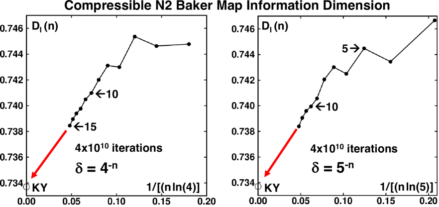
Figure 6: Stationary estimates for the Baker Map Information Dimension using up to $4^{15}$ and $5^{13}$ bins of equal width. These data, based on forty billion iterations of the random walk mapping suggest agreement with the Kaplan-Yorke dimensions of the one-dimensional $y$ version of two-panel Baker Maps, $D_{KY}=0.7337$.

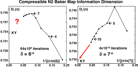
Figure 7: Stationary estimates for the one-dimensional version of the two-panel Baker Maps’ Information Dimensions using up to $6^{11}$ and $7^{11}$ bins of equal width. These data, like those in Figure 4, are based on forty billion iterations of the confined random-walk mapping. Both the Kaplan-Yorke dimension 0.7337 and the estimate 0.741 from Reference 14, based on meshes with up to $3^{19}$ equal bins, are shown as open circles at the left border of the $\delta=6^{-n}$ plot.

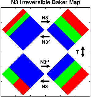
Figure 8: The three-panel Baker map $N3$ is slightly more complex than the two-panel $N2$ map, dividing the upper left red and green portion in half. Applying the sequence of three maps $N3TN3$ shown at the bottom left, is quite different to a mirror image of the original upper left. Evidently the $N3$ map is not time-reversible. But both the area-wise and the point-wise maps match the Kaplan-Yorke information dimension. Quite unlike the simpler two-panel Baker Map $N2$ the three routes to the $N3$ information dimension all reach the same value $D_{I}=0.78969$.

Inspection of Figure 9 shows that with mapping both the red and green panels increase in width by a factor 6 and decrease in length by a factor 3, while the blue panel, with probability 2/3, increases by a factor 3/2 and decreases by a factor 3, giving rise to the Kaplan-Yorke dimension

$$\lambda_{1}=+0.867563\ ;\ \lambda_{2}=-1.09861231\ \rightarrow$$

$$\lambda_{1}+0.78969\lambda_{2}=0\rightarrow D_{KY}=+1.789690\ ,$$

the same as the information dimensions found with area-wise and point-wise analyses. The probabilities associated with the $N3$ shown in the histograms of Figure 9 are identical to those of $N2$, but with a different ordering of the histogram rectangles. Evidently the $N3$ area-wise dimensionality, like the $N2$, doesn’t change. Unlike $N2$ the $N3$ map does agree with Kaplan-Yorke. In a memoir for Francis Ree, Bill chose meshes from $(1/3)^{5}$ to $(1/3)^{18}$ for a set of $10^{11}$ iterations of the $N3$ map. His Figure 7 appears to be fully consistent with a point-wise estimation $D_{I}=0.79$. Within the estimated uncertainty of 0.001 it appears that the $N3$ area-wise, point-wise, and Kaplan-Yorke values of the information dimension all agree with one another. This makes the failure of the simpler $N2$ Baker map, with only two linear panels, to provide simplicity a puzzling challenge.

Like $N2$ the three-panel $N3$ fractal corresponding to Figure 8 can be reproduced with calls to a random number generator. The simplest program results if the $N3$ fractal is generated in the $y$ direction or in the two-dimensional unit square, $0<x,y<1$:

call random_number(x)
             ynew = (1+y)/3 ! green
if(x.lt.1/6) ynew = (2+y)/3 ! red
if(x.gt.1/3) ynew = (0+y)/3 ! blue
call random_number(x)       ! if both (x,y) are desired

VIII Conclusions and Discussion

Relatively simple numerical work, on the order of a few dozen lines of FORTRAN, along with a few hours of laptop time, are enough to characterize the variety of results for $D_{I}$ based on [1] iterating areas or [2] generating representative sequences of points. These two different views of fractal structure are analogs of the Liouville and trajectory descriptions of particle mechanics. We think the singular anisotropy of fractals favors the pointwise approach. We found that pointwise analysis with the mesh series $(1/3)^{n}$ appears to contradict the Kaplan-Yorke dimension while the alternative series $(1/4)^{n},(1/5)^{n},(1/7)^{n}$ appear to support it. The series $(1/6)^{n}$ is inconclusive.

Though the one-dimensional confined random walk provides a fractal distribution in $\{y\}$, indistinguishable from that for the compressible $N2$ Baker Map, the confined-walk analog lacks the Baker-Map Lyapunov exponents on which the Kaplan-Yorke dimension relies :

$$\lambda_{1}=(1/3)\ln(27/4)\ ;\ \lambda_{2}=(1/3)\ln(2/27)\to D_{KY}=0.73368\ .$$

The variety of results obtained here for specific maps underlines the value of studying particular, as opposed to general, models. There are several publications suggesting that the information dimension is particularly robust to changes of variablesb11 , certainly a desirable property. On the other hand these results typically exclude mappings in which infinitely many points where mapping discontinuities occur, a characteristic of Baker maps.

Returning to the longstanding motivations of Loschmidt’s Reversibility Paradox and Zermélo’s Recurrence Paradox, compressible maps simplify our understanding of their resolutions, for flows just as well as for maps. Fractal states have zero volume in their embedding spaces. Chaos provides exponentially unstable (and therefore unobservable) repellors and exponentially stable (and therefore inevitable) attractors. Time-reversible maps provide simple fractal examples of Second Law irreversibility despite the paradoxes. Also notable is the quantitative agreement, within Central Limit Theorem fluctuations, of reversible distributions with those generated using stochastic random walks. Let us summarize the facts that stand out from our work: The simple $N2$ two-panel map, whether one-dimensional, in $y$, or two-dimensional, in $(q,p)$, provides three different values of information dimension “area-wise”, 0.78969 or 1.78969, “point-wise”, $0.741_{5}$ or $1.741_{5}$, and Kaplan-Yorke, 0.73368 or 1.73368. The more complex, but still linear, three-panel $N3$ map is consistent with $D_{I}=0.78969$ in one dimension and 1.78969 in two for all three approaches.

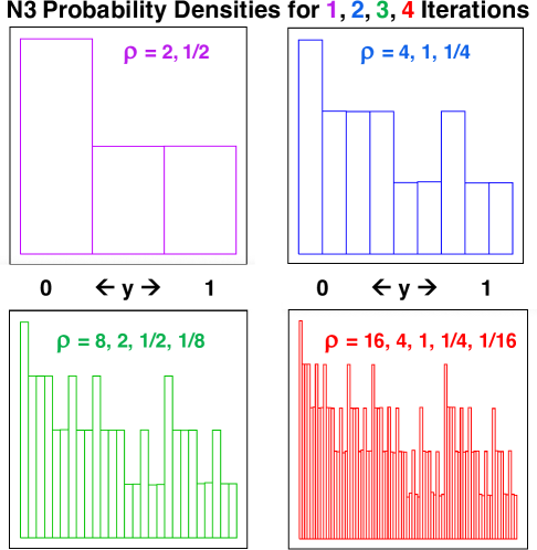
Figure 9: Histograms of the (base-4 logarithm of) probability density $\rho(y)$ for 1, 2, 3, and 4 area-wise iterations of the $y$ component of the nonequilibrium $N3$ Map. Notice that the central and rightmost thirds of each resulting mapping are both perfect scale models (reduced by a factor of four) of the leftmost third. This observation explains the persistence of the three-bin information dimension throughout any number of iterations.

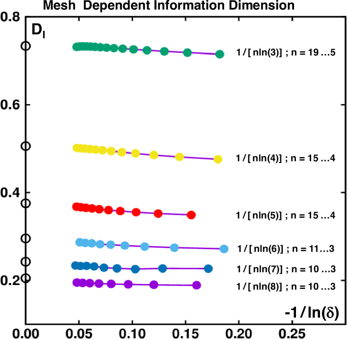
Figure 10: Dependence of the information dimension $D_{I}$ on the bin size $\delta$ for generalized Baker Maps. The integers from 3 to 8 indicate the fraction of the unit square occupied by the narrower rectangle of the mapping. As an example the $N2$ mapping of Figure 1 corresponds to the integer 3. The points for each mapping give information dimensions for different choices of the bin size, right-to-left from $(1/8)^{3}$ to $(1/8)^{10}$ for the bottom set of eight data points and from $(1/3)^{5}$ to $(1/3)^{19}$ for the top set of green points. The Kaplan-Yorke approximations are shown as open circles for each generalized map. They are excellent approximations! Each filled circle is the result of two billion steps in a random-walk simulation of the generalized Baker Map.

IX Acknowledgement

Carl Dettmann,Thomas Gilbert, and Kris Wojciechowski kindly provided helpful advice and references. Evidently the simplest generalized Baker Maps exhibit different area-wise and point-wise information dimensions. Surprisingly, it took us 20 years to come to this understanding. Thanks to our colleagues for their help along the way.

X Response to Comments by the Reviewers of March 2023

In early 2023 Tim Li requested that we contribute an article for a special issue of Entropy on “Maximum Entropy Random Walks”. This reminded us of our unpublished article of ours from September 2019, ”Random Walk Equivalence to the Compressible Baker Map and the Kaplan-Yorke Approximation to Its Information Dimension”. We brought that work up to date and submitted it to Entropy. Two reviewer comments soon arrived, one enthusiastic and the other not. The unfavorable review suggested that the manuscript had little to do with random walks or maximum entropy. We remark that our work was described by the favorable reviewer as including a novel, short, and highly-efficient random-walk algorithm to the evaluation of the ”information dimension” of maps chosen to shed light on the reversibility paradoxes of Loschmidt and Zermélo. Kaplan and Yorke formulated an approximate evaluation of the information dimensionb12 from the entropy of a set of points generated by an iterative solution of motion equations in the form of bin probabilities where the bins span the space occupied by solution points:

$$D_{I}=\sum P\ln P/\delta\simeq 1-(\lambda_{1}/\lambda_{2})=D_{KY},$$

where $P$ is the occupation probability of a bin of width $\delta$ and $D_{I}$ is the information dimension, a measure of the entropy of the set of points. Kaplan and Yorke’s formula for $D$ is much discussed in the literature, though the reasoning supporting it is obscure. We quote from page 169 of Tamás Tél’s and Márton Grioz’ excellent book, Chaotic Dynamicsb18 :

Both the information dimension and the average Lyapunov exponents are determined by the natural distribution. We can therefore expect to find an explicit relation between them. This rule, called the Kaplan-Yorke relation, is valid … [ ! ] for chaotic attractors of general two-dimensional invertible map, and can be obtained from a simple argument. [This is followed by two pages of informal text ending up with the “valid” rule $D=1-(\lambda_{1}/\lambda_{2})$.]

Because this “rule” is violated by the $N2$ map we do not reproduce the text supporting it. As one reviewer requests definitions of $P$ and the $\{\ \lambda_{i}\ \}$ we reiterate that $P$ is the probability of occupying a bin so that the sum over bins, $\sum P\equiv 1$, along with the usual formula for entropy, $S\propto-\sum P\ln P$ provides the information dimension of the point set in the limit that the bin size $\delta$ is small. The Lyapunov exponents, $N$ of them in an $N$-dimensional space, measure the exponential growth and shrinkage rates of a small comoving ball in phase space, ordered from the largest, in average value, to the most negative, so that a two-dimensional strange attractor set has a largest (positive) Lyapunov exponent $\lambda_{1}$ as well as a negative exponent, $\lambda_{2}$, with the sum negative, signaling the collapse of the set’s dimensionality below 2. The Kaplan-Yorke formula provides a fractional dimensionality between 1 and 2 (for a map) or 0 and 1 (for a confined random walk). In Figure 10 we display random-walk dimensions for six generalized Baker Maps (with mapping rectangles ranging from 1/3, as in our Figures 1 and 2, and 1/8, where the latter mapping provides a sevenfold change in area. A discussion by Doyne Farmer of similar map types can be found in Reference 20. Farmer analyzes the information dimension of a map similar to our $N2$ map (in his Figures 2 and 4) but does not distinguish point-wise and area-wise mappings as he was evidently unaware that the two can differ. For additional discussion of Lyapunov exponents and information dimension we refer the reader to Reference 18 and to the corresponding Wikipedia articles on the web.

References

- (1) B. L. Holian, W. G. Hoover, and H. A. Posch, “Resolution of Loschmidt’s Paradox: The Origin of Irreversible Behavior in Reversible Atomistic Dynamics”, Physical Review Letters 59, 10-13 (1987).
- (2) B. Moran, W. G. Hoover, and S. Bestiale, “Diffusion in a Periodic Lorentz Gas”, Journal of Statistical Physics 48, 709-726 (1987).
- (3) W. G. Hoover, H. A. Posch, B. L. Holian, M. J. Gillan, M. Mareschal, and C. Massobrio, “Dissipative Irreversibiity from Nosés Reversible Mechanics”, Molecular Simulation, 1, 79-86 (1987).
- (4) Wm. G. Hoover and H. A. Posch, “Chaos and Irreversibility in Simple Model Systems” 366-374 in Proceedings of Chaos and Irreversibility at Eötvös University 31 August- 6 September, 1997, organized by T. Tl, P. Gaspard, and G. Nicolis, Chaos 8, (1998).
- (5) H. A. Posch and W. G. Hoover, “Time-Reversible Dissipative Attractors In Three And Four Phase-Space Dimensions”, Physical Review E 55, 6803-6810 (1997)
- (6) S. Nosé, “A Molecular Dynamics Method for Simulations in the Canonical Ensemble”, Molecular Physics 52, 255-268 (1984).
- (7) S. Nosé, “A Unified Formulation of the Constant Temperature Molecular Dynamics Methods”, Journal of Chemical Physics 81, 511-519 (1984).
- (8) W. G. Hoover, “Canonical Dynamics: Equilibrium Phase-Space Distributions”, Physical Review A 31, 1695-1697 (1985).
- (9) H. A. Posch, W. G. Hoover, and F. J. Vesely, “Canonical Dynamics of the Nosé Oscillator: Stability, Order, and Chaos”, Physical Review A 33, 4253-4265 (1986).
- (10) W. G. Hoover and B. Moran, “Phase-Space Singularities in Atomistic Planar Diffusive Flow”, Physical Review A 40, 5319-5326 (1989).
- (11) J. D. Farmer, E. Ott, and J. A. Yorke, “The Dimension of Chaotic Attractors”, Physica 7 D, 153-180 (1983).
- (12) J. L. Kaplan and J. A. Yorke, “Chaotic Behavior of Multidimensional Difference Equations”, pages 204-227 in Functional Differential Equations and the Approximation of Fixed Points, edited by H. O. Peitgen and H. O. Walther (Springer, Berlin, 1979).
- (13) W. G. Hoover, C. G. Hoover, and F. Grond, “Phase-Space Growth Rates, Local Lyapunov Spectra, and Symmetry Breaking for Time-Reversible Dissipative Oscillators”, Communications in Nonlinear Science and Numerical Simulation 13, 1180-1193 (2006).
- (14) “Compressible Baker Maps and Their Inverses. A Memoir for Francis Hayin Ree [1936-2020]”, Computational Methods in Science and Technology 26, 5-13 (2020).
- (15) W. G. Hoover and C. G. Hoover, “Nonequilibrium Molecular Dynamics, Fractal Phase-Space Distributions, the Cantor Set, and Puzzles Involving Information Dimensions for Two Compressible Baker Maps”, Regular and Chaotic Dynamics 25, 412-423 (2020).
- (16) T. Tél, P. Gaspard, and G. Nicolis, “Chaos and Irreversibility: Introductory Comments”, Chaos 8, 309 (1998).
- (17) R. J. Fox, “Construction of the Jordan Basis for the Baker Map”, Chaos 7, 254-269 (1997).
- (18) T. Tél and M. Gruiz, Chaotic Dynamics; An Introduction Based on Classical Mechanics (Cambridge University Press, 2006).
- (19) J. Kumiĉák, “Irreversibility in a Simple Reversible Model”, Physical Review E, 016115 (2005).
- (20) J. D. Farmer, “Information Dimension and the Probabilistic Structure of Chaos”, Zeitschrift für Naturforschungen 3A, 1304-1325 (1982).