Untangling Optical Emissions of the Jet and Accretion Disk in the Flat-Spectrum Radio Quasar 3C 273 with Reverberation Mapping Data

Abstract

3C 273 is an intensively monitored flat-spectrum radio quasar with both a beamed jet and blue bump together with broad emission lines. The coexistence of the comparably prominent jet and accretion disk leads to complicated variability properties. Recent reverberation mapping monitoring for 3C 273 revealed that the optical continuum shows a distinct long-term trend that does not have a corresponding echo in the H$\beta$ fluxes. We compile multi-wavelength monitoring data from the Swift archive and other ground-based programs and clearly find two components of emissions at optical wavelength. One component stems from the accretion disk itself and the other component can be ascribed to the jet contribution, which also naturally accounts for the non-echoed trend in reverberation mapping data. We develop an approach to decouple the optical emissions from the jet and accretion disk in 3C 273 with the aid of multi-wavelength monitoring data. By assuming the disk emission has a negligible polarization in consideration of the low inclination of the jet, the results show that the jet contributes a fraction of $\sim$10% at the minimum and up to $\sim$40% at the maximum to the total optical emissions. This is the first time to provide a physical interpretation to the “detrending” manipulation conventionally adopted in reverberation mapping analysis. Our work also illustrates the importance of appropriately analyzing variability properties in cases of coexisting jets and accretion disks.

1 Introduction

3C 273 is an iconic object in extragalactic astronomy because of its historic role in discovering the first quasar and the first extragalactic radio jet (Hazard et al. 2018). It is classified to be a flat-spectrum radio quasar that has both a prominent blue bump together with broad emission lines, indicative of an accretion disk radiating at its nucleus (Paltani et al. 1998; Kriss et al. 1999; Türler et al. 1999; Soldi et al. 2008), and a beamed jet, a characteristic typical for blazar objects (Davis et al. 1991; Bahcall et al. 1995; Abraham, & Romero 1999; Perley & Meisenheimer 2017). However, unlike blazar objects, the optical polarization of 3C 273 is distinctively at low level (in average $p<$1%; Stockman et al. 1984; Berriman et al. 1990; Brindle et al. 1990; Marin 2014; Hutsemékers et al. 2018). These lines of observations make 3C 273 an archetype of active galactic nuclei (AGNs) in general and a good laboratory to study various (if not all) AGN phenomena in particular. With addition of its large brightness ($K$-band magnitude $\sim 10$) and mild proximity ($z=0.158$), 3C 273 had been intensively monitored and studied across almost all the wavelength bands (e.g., see Courvoisier 1998 for a review).

Table 1: Monitoring Data of 3C 273.

Source	Filter	Wavelength	Observation Period		$N_{\rm obs}$	$\Delta t_{\rm ave}$	$\Delta t_{\rm med}$	Ref
			JD-2,450,000	Date		(day)	(day)
Swift	UVW2	1928 Å	3562.152$-$8553.836	2005 Jul$-$2019 Mar	246	20.3	2.9	$\cdots$
Swift	UVM2	2246 Å	3562.152$-$8582.797	2005 Jul$-$2019 Apr	232	21.6	2.9	$\cdots$
Swift	UVW1	2600 Å	3562.152$-$8555.820	2005 Jul$-$2019 Mar	225	22.2	3.1	$\cdots$
Swift	U	3465 Å	3562.086$-$8580.789	2005 Jul$-$2019 Apr	194	25.9	1.9	$\cdots$
Swift	B Swift	4392 Å	3562.086$-$8304.324	2005 Jul$-$2018 Jul	111	42.7	1.1	$\cdots$
SMARTS	B	4450 Å	4677.497$-$7856.656	2008 Jul$-$2017 Apr	363	8.8	2.9	3
RM	$\cdots$	5100 Å	4795.018$-$8305.687	2008 Nov$-$2018 Jul	285	11.4	2.1	4
Swift	V Swift	5468 Å	3562.086$-$8304.324	2005 Jul$-$2018 Jul	225	21.1	1.9	$\cdots$
ASAS-SN	$V$	5510 Å	5956.146$-$8449.136	2012 Jan$-$2018 Nov	988	2.5	0.002	2
SMARTS	$V$	5510 Å	4677.499$-$7856.658	2008 Jul$-$2017 Apr	365	4.7	2.1	3
RM	$V$	5510 Å	4795.020$-$8305.697	2008 Nov$-$2018 Jul	306	11.9	2.0	4
SMARTS	$R$	6580 Å	4537.596$-$7856.660	2008 Jul$-$2017 Apr	371	8.9	2.9	3
SMARTS	$J$	12200 Å	4501.786$-$7091.743	2008 Feb$-$2015 Mar	306	8.5	2.1	3
OVRO	$\cdots$	200 $\mu$m	4473.983$-$8874.077	2008 Jan$-$2020 Jan	760	5.8	3.0	5

References. — (1) Drake et al. (2009); (2) Shappee et al. (2014) and Kochanek et al. (2017); (3) Bonning et al. (2012); (4) Zhang et al. (2019); (5) Richards et al. (2011).

The coexistence of the both comparably prominent jet and accretion disk results in the complicated emergent spectrum and variability properties (e.g., Stevens et al. 1998; Grandi & Palumbo 2004; Türler et al. 2006; Soldi et al. 2008; Chidiac et al. 2016; Plavin et al. 2019). By analyzing the monitoring data of the optical polarization, Impey et al. (1989) suggested that there is a miniblazar in 3C 273 that contributes about 10% of the optical flux densities. It is also this miniblazar component (with a high polarization) diluted by the disk emissions, leading to the low-level, highly variable polarization observed in 3C 273. For the blue bump of 3C 273, Paltani et al. (1998) proposed a decomposition of blue and red components. The former was explained by the thermal accretion disk emission and the latter was ascribed to the jet origin. Based on spectral fitting, Grandi & Palumbo (2004) similarly decomposed the X-ray spectrum of 3C 273 into two major contributions: a thermal component arising from the accretion disk and hot corona, and a non-thermal component arising from the jet.

Recently, Zhang et al. (2019) presented an optical reverberation mapping campaign for 3C 273 and found that the optical continuum shows a distinct long-term trend that does not have a corresponding echo in the light curves of the broad emission lines (including H$\beta$, H$\gamma$, and Fe II; see Figure 4 therein). This is in contradiction to the well observationally tested reverberation mapping scenario that broad emission lines stem from gaseous regions photoionized by the ionizing continuum and thereby the variations of broad emission lines closely follow these of the continuum (e.g., Peterson 1993). To alleviate biases in reverberation mapping analysis, Zhang et al. (2019) employed a linear polynomial to fit this long-term trend and artificially subtracted the best linear fit from the original light curve of the optical continuum (see also Wang et al. 2020). Such a “detrending” procedure was conventionally manipulated in the presence of non-echoed trends in reverberation mapping observations (Welsh 1999; Denney et al. 2010; Li et al. 2013; Peterson et al. 2014). However, to our best knowledge, there is not yet a satisfactory physical interpretation for this “detrending” operation.

Inspired by the above investigations, in this paper we link the non-echoed trend in 3C 273 with the jet contaminations at optical wavelength. The wealth of monitoring data and reverberation mapping observations for 3C 273 allows us to test for this possibility in a solid foundation. This is also a first attempt to give a physical explanation for the “detrending” operation in reverberation mapping analysis.

The paper is organized as follows. Section 2 collects publicly available monitoring data of 3C 273. Section 3 discusses several lines of evidence for the jet contaminations to the optical emissions. In Section 4, we develop a Bayesian decomposition framework and present the obtained results for decoupling the jet and disk emissions at optical wavelength. The discussions and conclusions are given in Sections 5 and 6, respectively. For the sake of brevity, when referring to the Julian Date, only the four least significant digits are retained.

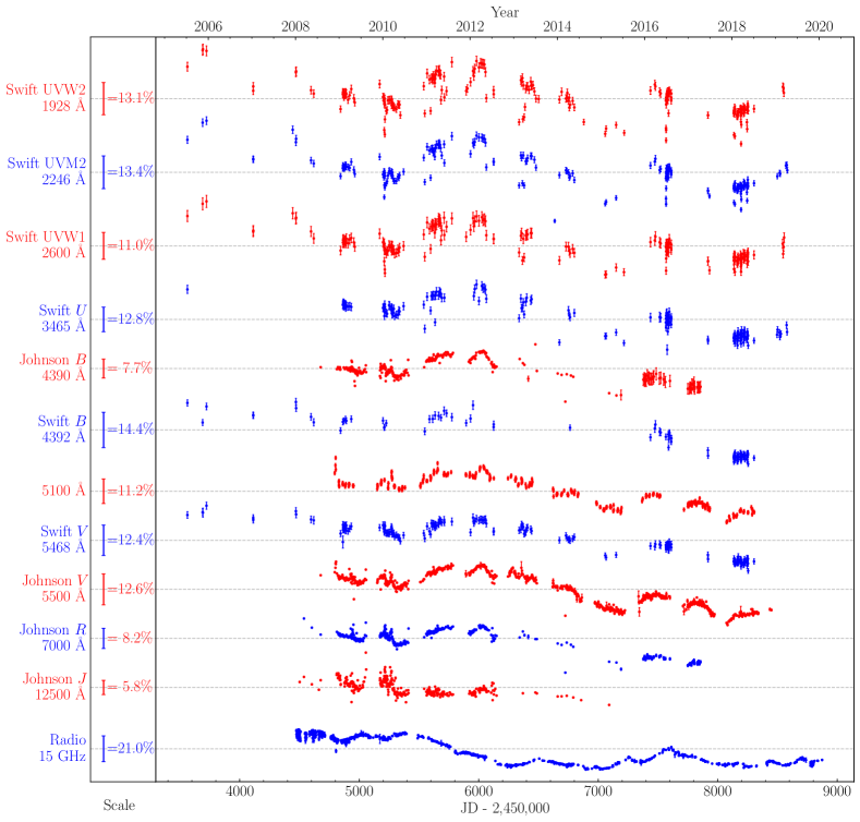
Figure 1: Compiled UV, optical, and radio continuum light curves of 3C 273. The scales along the vertical axis show the fractional variations of the corresponding light curves.

2 Data Compilation

In this section, we collect monitoring data of 3C 273 from various telescopes and sources. All the data compiled here are publicly accessible and most of them are directly usable except for the spectroscopic data and the archive UVOT data from the Swift telescope, which need extra reduction. For photometric data with the same filters, an intercalibration is required to account for different apertures adopted in different data sources. In Figure 1, we show all the compiled UV, optical, and radio continuum light curves.

2.1 Reverberation Mapping Data

Zhang et al. (2019) reported a reverberation mapping campaign for 3C 273 that synthesized the spectroscopic and photometric data from the Steward Observatory spectropolarimetric monitoring project (Smith et al. 2009) and the super-Eddington accreting massive black hole (SEAMBH) program (Du et al. 2014). The Steward Observatory project utilizes the 2.3 m Bok Telescope on Kitt Peak and the 1.54 m Kuiper Telescope on Mt. Bigelow in Arizona. The SEAMBH program utilizes the 2.4 m telescope at the Lijiang Station of the Yunnan Observatories, Chinese Academy of Sciences.

The campaign spanned from November 2008 to March 2018 and took a total of 296 epochs of observations. We directly use the light curves of the $V$-band photometry, 5100 Å flux densities, and H$\beta$ fluxes reduced by Zhang et al. (2019). As can be seen clearly in Figures 1 and 2, the light curves of the $V$-band photometry and 5100 Å flux densities show a long-term declining trend whereas the light curve of the H$\beta$ fluxes does not show such a trend, meaning that the H$\beta$ emission-line region does not reverberate to this long-term trend.

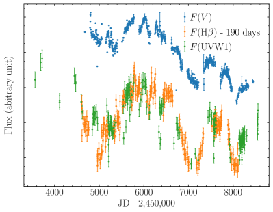
Figure 2: A comparison between the light curves of the H$\beta$ fluxes, Swift UVW1 band photometry, and Johnson $V$-band photometry. All the light curves are scaled and shifted for clarity and the H$\beta$ light curve is additionally shifted backward by a time of 190 days.

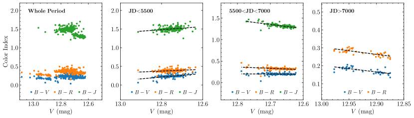
Figure 3: Color variations of 3C 273 with $V$-band magnitude using SMARTS data for the periods of the whole, JD$<$5500, 5500$<$JD$<$7000, and JD$>$7000 from the left to right panels, respectively. Dashed lines represent simple linear fits. In the rightmost panel, there are no $J$-band measurement points.

2.2 Optical/UV Photometric Data

Besides the $V$-band photometric data from the reverberation mapping campaign in Zhang et al. (2019), there are also other archival databases, monitoring programs, and time-domain surveys that cover 3C 273.

• The Small and Moderate Aperture Research Telescope System (SMARTS) monitoring program (Bonning et al. 2012). The program was conducted with the 1.3 m telescope at the Cerro Tololo Interamerican Observatory, which took photometry at five wavelength bands ($B$, $V$, $R$, $J$, $K$) simultaneously. This allow us to study the optical color variations of 3C 273. The $K$-band data has a relatively sparser cadence and we thus only use the other four band data.

• The All-Sky Automated Survey for Supernovae (ASAS-SN; Shappee et al. 2014; Kochanek et al. 2017). The ASAS-SN started to monitor 3C 273 at $V$-band since January 2012 and provides a real-time interface to access the $V$-band photometry. Typically, there are multiple exposures within one night and we combine those multiple exposures into one measurement.

• The Swift archive. The raw image data of six UVOT filters are open-access, covering the UV/optical from 1928 to 5468 Å. We reduced those raw data and measured the photometric fluxes (see Appendix A for the details of data reduction). We excluded those apparently problematic points which were considered to be caused by the contamination of dust and/or other debris within the instrument (Edelson et al. 2015) and finally obtained about 230 epochs of measurements that span from July 2005 to March 2019 for each filters.

To convert magnitudes to flux densities, we adopt the zero-magnitude points for $B$, $V$, $R$, and $J$ bands determined by Johnson (1966) as follows: $F(B=0)=7.20$, $F(V=0)=3.92$, $F(R=0)=1.76$, and $F(J=0)=0.34$, all with a unit of $10^{-9}{\rm~{}erg~{}s^{-1}~{}cm^{-2}~{}\text{\AA}^{-1}}$. In addition, we need to intercalibrate the photometry at Johnson $V$-band from different sources. To this end, we first select the SMARTS $V$-band photometry as the reference set and then apply a scale factor ($\varphi$) and flux adjustment ($G$) to the flux densities of the other sources as (e.g., Peterson et al. 1995; Li et al. 2014)

$$F(V)=\varphi F(V)_{\rm obs}+G.$$ (1)

As such, the light curves from all the sources are aligned into a common scale. Here, the values of $\varphi$ and $G$ are determined by comparing the closely spaced measurements within 5 days from two data sources. Note that we do not align the Swift $V$-band photometry with the other Johnson $V$-band photometry. The intercalibrated $V$-band light curve is also shown in Figure 1.

2.3 Radio Data

We use the radio data from the large-scale, fast-cadence 15 GHz monitoring program with the 40 m telescope at the Owens Valley Radio Observatory (Richards et al. 2011), which began in late 2007 and had a nearly daily cadence (but with seasonal gaps). The program is still ongoing and the latest released data was to Jan 28, 2020. There are in total 760 epochs of observations by the time of writing.

In Table 1, we summarize the basic properties of all the compiled light curve data.

3 Evidence for Jet Contaminations

Using the monitoring data collected above, in this section we present four pieces of evidence that the jet emissions at optical wavelengths are non-negligible.

3.1 UV and Optical Variations

In Figure 2, we compare the light curve of the H$\beta$ fluxes with these at the $V$-band and Swift UVW1 band. Previous reverberation mapping observations for H$\beta$ lines had well established that H$\beta$ lines respond to (UV) continuum variations with a time delay due to the light traveling time from the central continuum sources to the broad-line regions (Kaspi et al. 2000; Bentz et al. 2013; Du et al. 2016). The H$\beta$ light curve is therefore scaled and shifted in both flux and time to align with the UV light curve. We can find that the variation patterns generally match with each other. This is consistent with the simple photoionization theory that broad emission lines are reprocessed emissions from the gaseous regions photoionized by the central UV/X-ray ionizing photons. Therefore, emission line variations are just blurred echoes of the ionizing continuum variations with time delays arising from light traveling times between the ionizing source and gaseous regions.

On the contrary, the $V$-band light curve shows a distinct long-term declining trend that is absent in the H$\beta$ and UVW1 light curves. Previous multi-wavelength continuum monitoring of AGNs had clearly demonstrated that AGN variations are tightly correlated throughout UV and optical bands (e.g., Edelson et al. 2019). Such a distinct variation trend in 3C 273 strongly suggests that in addition to the accretion disk emission, there has to be another independent component that contributes to the optical emissions.

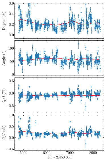
Figure 4: Variability of the optical integrated polarizations of 3C 273 measured by the Steward Observatory spectropolarimetric monitoring project (Smith et al. 2009). From top to bottom panels are polarization degree, polarization angle, and the Stokes parameters $Q/I$ and $U/I$, respectively. Solid lines with shaded areas represent the best fits of our decomposition procedure (see Section 4.3 for a detail).

3.2 Color Variations

Figure 3 shows the color variations ($B-V$, $B-R$, and $B-J$) of 3C 273 with the $V$-band magnitude using the SMARTS data (Bonning et al. 2012). All the three color indices vary with a complicated, time-dependent behaviour. For the sake of comparison, we divide the light curves into three segments (JD$<$5500, 5500$<$JD$<$7000, and JD$>$7000) and plot the corresponding color indices in the right three panels of Figure 3. For the period of JD$<$5500, the color indices increase as the $V$-band magnitude decreases, indicating that 3C 273 become redder when brighter. By contrast, for the periods of 5500$<$JD$<$7000 and JD$>$7000, the variation behaviours are conversed, namely, 3C 273 becomes bluer when brighter. The differences between the periods of 5500$<$JD$<$7000 and JD$>$7000 are 1) the typical values of the color indices are not the same, as can be seen in the leftmost panel of Figure 3; and 2) the slopes of the color indices with the $V$-band magnitude are also not the same.

A number of previous studies had also investigated the color variability of 3C 273 on various time scales (e.g., Dai et al. 2009; Ikejiri et al. 2011; Fan et al. 2014; Xiong et al. 2017; Zeng et al. 2018). Those studies basically found that the color variability of 3C 273 seems to transit between the bluer-when-brighter and redder-when-brighter trends, plausibly depending on the observed epochs and brightness states. Our results are generally consistent with those reported behaviours.

There is consensus from large AGN samples that radio-quiet AGNs generally exhibit the bluer-when-brighter trend (e.g., Schmidt et al. 2012; Ruan et al. 2014; Guo & Gu 2016), whereas in radio AGNs, both the bluer-when-brighter and redder-when-brighter trends are observed (e.g., Gu et al. 2006; Rani et al. 2010; Bian et al. 2012). The above observations imply that sole disk variability cannot explain the complicated color variation behaviours in 3C 273.

3.3 Polarization Variations

Figure 4 plots the optical polarization degree and polarization angle of 3C 273 (5000-7000Å) measured by the Steward Observatory spectropolarimetric monitoring project (Smith et al. 2009). Similar with normal radio-quiet AGNs (Stockman et al. 1984; Brindle et al. 1990; Marin 2014; Hutsemékers et al. 2018), 3C 273 overall exhibits a low-level optical polarization of $p\sim$0.2% in average, with the maximum up to $p\gtrsim 0.6\%$. However, the polarization strikingly undergoes large variations with $\Delta p/p>1$, a characteristic typically observed in blazar-like AGNs (Impey et al. 1989). Meanwhile, the polarization angle also varies mildly with time.

For normal radio-quiet AGNs, low-level polarizations are generally believed to originate from scattering of dust grains in torus or free electrons distributed somewhere in AGNs (Stockman et al. 1984; Smith et al. 2002; Goosmann & Gaskell 2007, and references therein). The such resulting (linear) polarizations are not expected to show large variability in amount or orientation (Rudy et al. 1983; Stockman et al. 1984), which is generally supported by polarization observations for normal radio-quiet AGNs (e.g, Stockman et al. 1984; Berriman et al. 1990; Brindle et al. 1990; Marin 2014). In this sense, the variable polarization degree and angle shown in Figure 4 directly indicates non-negligible contributions of synchrotron emissions from the jet at optical wavelength (Impey et al. 1989).

3.4 Detrending the Optical Continuum Emission

As illustrated in Figure 2, the optical light curve displays an extra long-term trend compared to the UV and H$\beta$ light curves. Also, through simple shifting and scaling, the variation patterns of the UV and H$\beta$ light curves are well matched. In consideration of the high cadence of the H$\beta$ light curve, below we use it as a proxy for the UV light curve. We artificially scale and shift the H$\beta$ light curve as

$$\tilde{f}({\rm H}\beta)=2.5\times\frac{F({\rm H}\beta)}{\bar{F}({\rm H}\beta)}-1.8,$$ (2)

where $\bar{F}({\rm H}\beta)$ is the mean of the H$\beta$ light curve. The numbers in the above equation is chosen for the purpose of illustration and do not have special meanings. We then subtract $\tilde{f}({\rm H}\beta)$ from the scaled $V$-band light curve

$$\tilde{f}(V)=\frac{F(V)}{\bar{F}(V)},$$ (3)

and obtain the residuals

$$\Delta\tilde{f}=\tilde{f}(V)-\tilde{f}({\rm H}\beta),$$ (4)

where $\bar{F}(V)$ is the mean of the $V$-band light curve. Figure 5 plots $\tilde{f}({\rm H}\beta)$ and $\tilde{f}(V)$ in the top panel and $\Delta\tilde{f}$ in the bottom panel. It is remarkable that the variation pattern of the residual light curve highly resembles that of the radio light curve. To guide the eye, we also superpose the scaled radio light curve in the bottom panel of Figure 5. After shifting backward about 500 days, the radio light curve well matches the residual light curve. This strongly suggests that the jet contamination is a plausible origin of the extra long-term trend in the optical light curve.

In the above, we scale and shift the light curves artificially for illustration purpose. In reality, the relations among these light curves are by no means such simple, for example, according to line reverberation mapping scenario, the H$\beta$ emission is linked to the UV continuum by convolving with a transfer function (e.g., Peterson 1993). Below, we develop a framework to untangle the optical jet and disk emissions in a rigorous mathematical foundation.

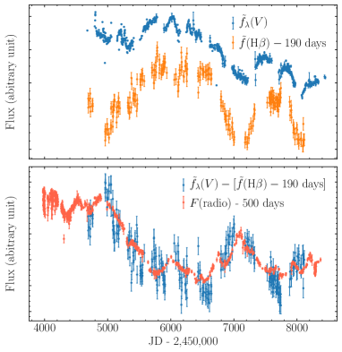
Figure 5: (Top) The scaled $V$-band light curve denoted by $\tilde{f}(V)$ and scaled and shifted H$\beta$ light curve denoted by $\tilde{f}({\rm H\beta})$. (Bottom) The residuals $\tilde{f}(V)-\tilde{f}({\rm H\beta})$, on which superposed is the scaled radio 15 GHz light curve denoted by $F(\rm radio)$. Note that $\tilde{f}({\rm H\beta})$ and $F(\rm radio)$ are additionally shifted backward by 190 and 500 days, respectively. See 3.4 for the definitions of $\tilde{f}(V)$ and $\tilde{f}({\rm H\beta})$.

Table 2: Free Parameters.

Parameter	Prior	Range	Definition
$\sigma_{\rm d}$	Logarithmic	($10^{-5}$, 1.0)	Long-term standard deviation of the optical disk emission
$T_{\rm d}$	Logarithmic	(1.0, $10^{5}$) days	Characteristic damping time scale of the optical disk emission
$\sigma_{\rm j}$	Logarithmic	($10^{-5}$, 1.0)	Long-term standard deviation of the optical jet emission
$T_{\rm j}$	Logarithmic	(1.0, $10^{5}$) days	Characteristic damping time scale of the optical jet emission
$f_{\rm H\beta}$	Logarithmic	($10^{-3}$, $10^{3}$)	Amplitude of the Gaussian transfer function for the H$\beta$ light curve
$\tau_{\rm H\beta}$	Uniform	(0, 300) days	Mean time delay of the Gaussian transfer function for the H$\beta$ light curve
$\omega_{\rm H\beta}$	Logarithmic	(0, 1000) days	Standard deviation of the Gaussian transfer function for the H$\beta$ light curve
$f_{\rm j}$	Logarithmic	($10^{-3}$, $10^{3}$)	Amplitude of the Gaussian transfer function for the 15 GHz radio light curve
$\tau_{\rm j}$	Uniform	(0, 1000) days	Mean time delay of the Gaussian transfer function for the 15 GHz radio light curve
$\omega_{\rm j}$	Logarithmic	(0, 1000) days	Standard deviation of the Gaussian transfer function for the 15 GHz radio light curve
$f_{q}$	Uniform	(0, 1)	Ratio of the mean of the disk emission to that of the total optical emission
$\bar{p}_{\rm j}$	Uniform	(0, 2)%	Averaged polarization degree of the optical jet emission
$\bar{\theta}_{\rm j}$	Uniform	(0, 180∘)	Averaged polarization angle of the optical jet emission

Note. — The prior ranges for $\sigma_{\rm d}$, $\sigma_{\rm j}$, $f_{\rm H\beta}$, and $f_{\rm j}$ are assigned in terms of the mean fluxes of all the light curves normalized to unity. A “logarithmic” prior means a uniform prior for the logarithm of the parameter. In real calculations, parameters with logarithmic priors are reparameterized by their logarithms.

4 Untangling the Jet and Disk Emissions

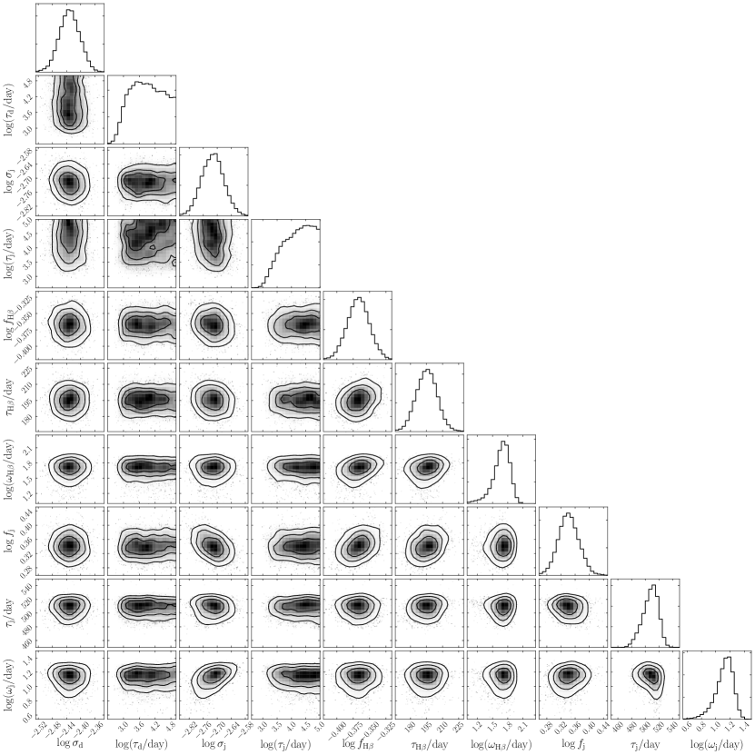
Figure 6: One- and two-dimensional distributions of the free parameters. The contours are at 1$\sigma$, 1.5$\sigma$, and 2$\sigma$ levels. This figure is made using the Python module corner.py (Foreman-Mackey 2016).

4.1 Basic Equations

The observed optical emission is deemed to be a combination of the disk and jet emissions, namely,

$$C_{\rm t}(t)=C_{\rm d}(t)+C_{\rm j}(t),$$ (5)

where the subscripts “t”, “d”, and “j” represent the total, disk, and jet emissions, respectively. According to the generic jet scenario (e.g., Marscher & Gear 1985; Türler et al. 2000), perturbations propagate along jet from denser to less denser regions and the emitted photon energy gradually decreases from $\gamma$/X-ray, UV/optical to radio wavelengths. With this scenario, the jet emissions at optical and radio wavelengths are linked with a transfer function (also called delay map) as

$$R_{\rm j}(t)=\int\Psi_{\rm j}(\tau)C_{\rm j}(t-\tau)d\tau,$$ (6)

where $R_{\rm j}(t)$ is flux at radio band and $\Psi_{\rm j}(\tau)$ is the transfer function at the time delay $\tau$. The H$\beta$ emission line responds to the continuum emission from the accretion disk as (Peterson 1993)

$$L_{\rm H\beta}(t) = \int\Psi_{\rm H\beta}(\tau)C_{\rm d}(t-\tau)d\tau,$$ (7)

where $L_{\rm H\beta}(t)$ is the line flux and $\Psi_{\rm H\beta}(\tau)$ is the transfer function of the BLR.

By appropriately solving Equations (5-7), we can separate the optical emissions from the disk $C_{\rm d}(t)$ and the jet $C_{\rm j}(t)$. However, this is challenging as the transfer functions $\Psi_{\rm j}$ and $\Psi_{\rm d}$ are fully unknown. Below we proceed with several simple, but physically reasonable assumptions and show how to recover the disk and jet emissions as well as the two transfer functions based on the framework of linear reconstruction of irregularly sampled time series outlined by Rybicki & Press (1992).

First, we assume that time variations of the disk and jet emissions are described by two independent damped random walk (DRW) processes. DRW processes have been applied to various time series data with their capability of capturing main variation features (e.g. Kelly et al. 2009; Zu et al. 2011; Pancoast et al. 2014; Li et al. 2014, 2016, 2018). A DRW process is a stationary Gaussian process and its covariance between times $t_{k}$ and $t_{m}$ damps exponentially with the time difference $\Delta t=t_{m}-t_{k}$. As such, the auto-covariance functions of $C_{\rm d}(t)$ and $C_{\rm j}(t)$ are given by

$$S_{\rm dd}(\Delta t) = \left\langle C_{\rm d}(t_{k})C_{\rm d}(t_{m})\right\rangle=\sigma_{\rm d}^{2}\exp\left(-\frac{|\Delta t|}{T_{\rm d}}\right),$$ (8)

$$S_{\rm jj}(\Delta t) = \left\langle C_{\rm j}(t_{k})C_{\rm j}(t_{m})\right\rangle=\sigma_{\rm j}^{2}\exp\left(-\frac{|\Delta t|}{T_{\rm j}}\right),$$ (9)

where the angle brackets represent the statistical ensemble average, $T_{\rm d}$ and $T_{\rm j}$ are the characteristic damping time scales, and $\sigma_{\rm d}$ and $\sigma_{\rm j}$ are the long-term standard deviations of the disk and jet emissions, respectively.

From the fundamental plane of black hole activity (e.g., Merloni et al. 2003), we know that there must be somehow disk-jet connection over the lifetime of the black hole activity, which is typically on the order of million years (e.g., Martini 2004). Nevertheless, the assumption that $C_{\rm d}(t)$ and $C_{\rm j}(t)$ are independent still stands reasonable in the sense that we are only concerned with variations on a much shorter timescale ($\sim$ years), which are most likely driven by independent fluctuations/perturbations in the disk and jet. Since $C_{\rm d}(t)$ and $C_{\rm j}(t)$ are independent, their covariance is simply zero. The auto-covariance function of $C_{\rm t}(t)$ is thereby

$$S_{\rm tt}(\Delta t)=\left\langle C_{\rm t}(t_{k})C_{\rm t}(t_{m})\right\rangle=S_{\rm dd}(\Delta t)+S_{\rm jj}(\Delta t).$$ (10)

Second, for simplicity, we assume that the transfer functions $\Psi_{\rm j}(\tau)$ and $\Psi_{\rm d}(\tau)$ are parameterized by Gaussians (see also Section 5.3 below),

$$\Psi_{\rm H\beta}(\tau)=\frac{f_{\rm H\beta}}{\sqrt{2\pi}\omega_{\rm H\beta}}\exp\left[-\frac{(\tau-\tau_{\rm H\beta})^{2}}{2\omega^{2}_{\rm H\beta}}\right],$$ (11)

and

$$\Psi_{\rm j}(\tau)=\frac{f_{\rm j}}{\sqrt{2\pi}\omega_{\rm j}}\exp\left[-\frac{(\tau-\tau_{\rm j})^{2}}{2\omega^{2}_{\rm j}}\right],$$ (12)

where ($f_{\rm H\beta}$, $\tau_{\rm H\beta}$, $\omega_{\rm H\beta}$) and ($f_{\rm j}$, $\tau_{\rm j}$, $\omega_{\rm j}$) are free parameters. By this definition, $\tau_{\rm H\beta}$ and $\tau_{\rm j}$ represent the time delays of the H$\beta$ emission and radio emission relative to the optical emission, respectively. With Gaussian transfer functions, the covariances among $C_{\rm t}(t)$, $R_{\rm j}(t)$, and $L_{\rm H\beta}(t)$ can be expressed analytically by the aid of error function (see Appendix B).

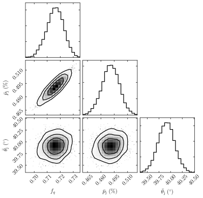
Figure 7: The posterior distributions of $f_{q}$, $\bar{p}_{\rm j}$, and $\bar{\theta}_{\rm j}$. The contours are at 1$\sigma$, 1.5$\sigma$, and 2$\sigma$ levels. This figure is made using the Python module corner.py (Foreman-Mackey 2016).

4.2 Bayesian Inference

The observation data at hand are the optical continuum $C_{\rm t}(t)$, the radio flux $R_{\rm j}(t)$, the H$\beta$ emission line flux $L_{\rm H\beta}(t)$, and their respective associated measurement uncertainties. For brevity, we join [$C_{\rm t}(t)$, $R_{\rm j}(t)$, $L_{\rm H\beta}(t)$] to a vector and denote it by $\mathbi{y}$. By assuming that the measurement noises are Gaussian, the likelihood probability for $\mathbi{y}$ is (Rybicki & Press 1992; Zu et al. 2011; Li et al. 2013)

$$P(\mathbi{y}|\boldsymbol{\theta}) = \frac{1}{\sqrt{(2\pi)^{m}|\mathbi{C}||\mathbi{E}^{T}\mathbi{C}^{-1}\mathbi{E}|}}$$ (13)

$$\times \exp\left[-\frac{(\mathbi{y}-\mathbi{E\hat{q}})^{T}\mathbi{C}^{-1}(\mathbi{y}-\mathbi{E\hat{q}})}{2}\right],$$

where $\boldsymbol{\theta}$ denotes all the free parameters, $m$ is the total number of data points in $\mathbi{y}$, $\mathbi{C}=\mathbi{S}+\mathbi{N}$, $\mathbi{S}$ is the covariance matrix of $\mathbi{y}$, $\mathbi{N}$ is the covariance matrix of the measurement noises, $\mathbi{\hat{q}}$ is a vector with three entries that represent the best estimate for the means of $\mathbi{y}$,

$$\mathbi{\hat{q}}=(\mathbi{E}^{T}\mathbi{C}^{-1}\mathbi{E})^{-1}\mathbi{E}^{T}\mathbi{C}^{-1}\mathbi{y},$$ (14)

and $\mathbi{E}$ is a $3\times m$ matrix with entries of $(1,0,0)$ for the optical continuum data points, $(0,1,0)$ for the radio data points, and $(0,0,1)$ for the H$\beta$ flux data points.

The posterior probability for the free parameters $\boldsymbol{\theta}$ is

$$P(\boldsymbol{\theta}|\mathbi{y})=\frac{P(\mathbi{y}|\boldsymbol{\theta})P(\boldsymbol{\theta})}{P(\mathbi{y})},$$ (15)

where $P(\mathbi{y})$ is the marginal likelihood and $P(\boldsymbol{\theta})$ is the prior probability of the free parameters. The prior probabilities for $\tau_{\rm H\beta}$ and $\tau_{\rm j}$ are set to be uniform and for the other parameters are set to be a logarithmic prior. Table 2 lists the priors for all the free parameters. We employ the diffusive nested sampling technique (Brewer et al. 2011) to explore the posterior probability and construct posterior samples to determine the best estimates and uncertainties for the free parameters. With the best estimated parameters, a reconstruction of $\mathbi{y}$ is given by

$$\mathbi{\hat{y}}=\mathbi{SC}^{-1}(\mathbi{y-E\hat{q}})+\mathbi{E\hat{q}}.$$ (16)

Table 3: Inferred Parameter Values and Uncertainties.

Parameter	Value
$\log\sigma_{\rm d}$	$-2.430_{-0.028}^{+0.028}$
$\log(T_{\rm d}/{\rm day})$	$3.92_{-0.67}^{+0.71}$
$\log\sigma_{\rm j}$	$-2.717_{-0.046}^{+0.042}$
$\log(T_{\rm j}/{\rm day})$	$4.28_{-0.61}^{+0.49}$
$\log f_{\rm H\beta}$	$-0.367_{-0.016}^{+0.016}$
$\tau_{\rm H\beta}/{\rm day}$	$195.4_{-9.2}^{+8.6}$
$\log(\omega_{\rm H\beta}/{\rm day})$	$1.69_{-0.20}^{+0.12}$
$\log f_{\rm j}$	$0.341_{-0.026}^{+0.028}$
$\tau_{\rm j}/{\rm day}$	$509.2_{-12.8}^{+8.0}$
$\log(\omega_{\rm j}/{\rm day})$	$1.143_{-0.130}^{+0.084}$
$f_{q}$	$0.716_{-0.006}^{+0.006}$
$\bar{p}_{\rm j}/\%$	$0.491_{-0.009}^{+0.009}$
$\bar{\theta}_{\rm j}/^{\circ}$	$39.91_{-0.17}^{+0.17}$

Note. — Parameter values are determined from the medians of the posterior probability distributions and the uncertainties represent the 68.3% confidence intervals. The values of $f_{q}$, $\bar{p}_{\rm j}$, and $\bar{\theta}_{\rm j}$ are given by fixing the interstellar polarization degree and angle to $\theta_{\star}=0.15\%$ and $\theta_{\star}=70^{\circ}$.

It is worth stressing that the likelihood probability $P(\mathbi{y}|\boldsymbol{\theta})$ in Equation (13) are fully determined without involving extra parameters that we will introduce below to untangle the mean fluxes of the disk and jet emissions. Therefore, at this point we can already obtain the posterior samples for the free parameters defined above by optimizing the posterior probability $P(\boldsymbol{\theta}|\mathbi{y})$ in Equation (15). This means that we can “detrend” the light curves to determine the time delays ($\tau_{\rm H\beta}$ and $\tau_{\rm j}$) without invoking the need of knowing the mean fluxes of individual emission components.

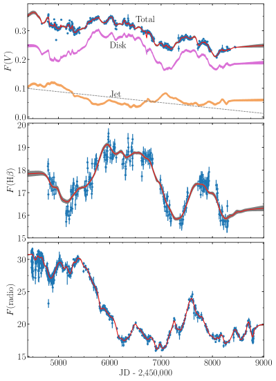
Figure 8: Best fits to the $V$-band, H$\beta$, and radio light curves. Points with error bars represent the observed data and red lines with shaded areas represent the best fits. In the top panel, superposed are the decomposed disk and jet light curves. Grey dashed line represents the linear polynomial used to detrend the continuum light curve by Zhang et al. (2019), which is shifted vertically to guide the eye.

4.3 Including the Polarization Data

In Equation (16), there involve the means $\mathbi{\hat{q}}$ of the light curves, which are calculated by Equation (14). This implies that when reconstructing $C_{\rm j}(t)$ and $C_{\rm d}(t)$, their means are degenerated since we only know the sum of $C_{\rm j}(t)$ and $C_{\rm d}(t)$, namely $C_{\rm t}(t)$. We define a free parameter $f_{q}$ to denote the ratio of the mean of the disk emission to that of the total optical emission. With this definition, we reconstruct $C_{\rm j}(t)$ and $C_{\rm d}(t)$ as

$$\mathbi{\hat{y}}_{\rm d}=\mathbi{S_{\rm d*}C}^{-1}(\mathbi{y-E\hat{q}})+f_{q}\mathbi{E}\hat{q}_{\rm t},$$ (17)

and

$$\mathbi{\hat{y}}_{\rm j}=\mathbi{S_{\rm j*}C}^{-1}(\mathbi{y-E\hat{q}})+(1-f_{q})\mathbi{E}\hat{q}_{\rm t},$$ (18)

where $\hat{q}_{\rm t}$ is the mean of $C_{\rm t}(t)$, $\mathbi{S_{\rm d*}}$ and $\mathbi{S_{\rm j*}}$ are covriances of $C_{\rm d}(t)$ and $C_{\rm j}(t)$ with the observed light curves $\mathbi{y}$ at reconstructed times, respectively.

The restriction that both $C_{\rm j}(t)$ and $C_{\rm d}(t)$ must be positive can constrain $f_{q}$ to a generic range of $f_{q}\sim(0.18-0.83)$. To further constrain the value of $f_{q}$, we resort to the polarization data shown in Figure 4. The observed optical polarization is deemed to be a combination of interstellar polarization and polarizations of the disk and jet emissions. As usual, we depict polarization using the Stokes parameters ($I,Q,U,0$) ($V=0$ for linear polarization; e.g., Chandrasekhar 1960). The optical polarization of 3C 273 is then given by

$$I = C_{\rm t}=C_{\rm d}+C_{\rm j},$$ (19)

$$Q = C_{\rm d}p_{\rm d}\cos(2\theta_{\rm d})+C_{\rm j}p_{\rm j}\cos(2\theta_{\rm j})+C_{\rm t}p_{\star}\cos(2\theta_{\star}),$$ (20)

$$U = C_{\rm d}p_{\rm d}\sin(2\theta_{\rm d})+C_{\rm j}p_{\rm j}\sin(2\theta_{\rm j})+C_{\rm t}p_{\star}\sin(2\theta_{\star}),$$ (21)

where $p$ and $\theta$ represent polarization degree and position angle, and the subscripts “d”, “j”, and “$\star$” represent disk, jet, and interstellar polarization, respectively. The polarization degree and angle of the total emission are then calculated as

$$p = \frac{\sqrt{U^{2}+Q^{2}}}{I},$$ (22)

$$\theta = \frac{1}{2}\tan^{-1}\left(\frac{U}{Q}\right).$$ (23)

It is expected that the interstellar polarization is constant while the polarizations of the disk and jet emissions might vary with time. In addition, there might be a time delay between the polarized and unpolarized disk emissions depending on the location of scattering materials (e.g. Gaskell et al. 2012; Rojas Lobos et al. 2020).

The interstellar polarization degree can be estimated by an approximation $p_{\star}(\%)=0.3E(B-V)$ (Rudy et al. 1983). The reddening for 3C 273 is $E(B-V)=0.05$ mag (Wu 1977), leading to an interstellar polarization of $p_{\star}=0.15\%$. This crude estimate is generally consistent with the observational constraints of $\sim 0.17\%$ by Impey et al. (1989) and $\sim 0.13\%$ by Smith et al. (1993). The correspondingly estimated position angle of the interstellar polarization is $\theta_{\star}\sim 80^{\circ}$ by Impey et al. (1989) and $\theta_{\star}\sim 60^{\circ}$ by Smith et al. (1993). We hereafter use the medians $p_{\star}=0.15\%$ and $\theta_{\star}=70^{\circ}$ as the fiducial values for the interstellar polarization.

For disk emissions, there have been several studies that calculated polarizations arising from scattering by electrons in disk atmospheres (Chandrasekhar 1960; Phillips & Meszaros 1986; Agol & Blaes 1996; Beloborodov 1998; Li et al. 2009) or by dust grains/electrons distributed beyond the disk (such as in torus or polar regions; Wolf & Henning 1999; Goosmann & Gaskell 2007; Rojas Lobos et al. 2018). All those calculations showed that the polarization of disk emissions strongly depends on the view inclination of the disk. As the inclination approaches face-on ($i\rightarrow 0$), the polarization decreases to zero because of symmetry. We note that observations of the superluminal motion of the radio jet of 3C 273 yielded an inclination angle of $i\sim 10^{\circ}$ (Abraham, & Romero 1999; Savolainen et al. 2006; Jorstad et al. 2017). If we assume that the jet is aligned with the disk’s rotation axis, the inclination angle of the disk would be also $\sim 10^{\circ}$. For an optically thick disk with pure scattering, such an inclination results in a quite low degree of polarization $\sim$0.05% (Chandrasekhar, 1960, Section X). Once taking into account photon absorption, this degree of polarization will be further reduced as absorption tends to destroy the polarization of photons. The calculations of Beloborodov (1998) showed that the presence of a fast wind flowing away from the accretion disk will alter the disk’s intrinsic polarization and produce a high polarization degree at large inclination angles. However, at low inclination angles, the effect of a disk wind is again insignificant (see Figure 2 therein). For cases of polarization caused by scattering of dust grains/electrons distributed beyond the accretion disk, the studies of Wolf & Henning (1999) and Goosmann & Gaskell (2007) also generally indicated a pretty low degree of polarization at inclination of $i\sim 10^{\circ}$. Taken the above together, we neglect the polarization of disk emissions by default ($p_{\rm d}=0$) and below we will discuss the influences on our conclusions if the polarization of disk emissions is not negligible.

Equations (19-21) implies that the time-dependent ratio $C_{\rm j}(t)/C_{\rm t}(t)$ does contribute to the observed polarization variability. In generic, both the polarization degree $p_{\rm j}$ and angle $\theta_{\rm j}$ can change with time. In such a case, Equations (19-21) cannot uniquely determine $f_{\rm q}$ and time-dependent $p_{\rm j}$ and $\theta_{\rm j}$. As illustrated below, the global variation patterns of the observed polarization degree (plotted in Figure 4) are generally similar to these of the ratio $C_{\rm j}(t)/C_{\rm t}(t)$, except for patterns in short timescales within about one year. This motivates us to make a assumption that the global variations of the observed polarizations are mainly contributed from the ratio $C_{\rm j}(t)/C_{\rm t}(t)$ whereas the intrinsic variations of the jet polarizations are mainly responsible for the short-timescale variations. As such, by using Equations (19-21) to fit the observed $Q$ and $U$ (see Figure 4), we can uniquely determines $f_{\rm q}$ and the averaged values of $p_{\rm j}(t)$ and $\theta_{\rm j}(t)$, which we denote as $\bar{p}_{\rm j}$ and $\bar{\theta}_{\rm j}$, respectively. The priors for $f_{q}$, $\bar{p}_{\rm j}$, and $\bar{\theta}_{\rm j}$ are listed in Table 2.

We stress again that the likelihood probability $P(\mathbi{y}|\boldsymbol{\theta})$ in Equation (13) does not involve $f_{q}$, $\bar{p}_{\rm j}$, and $\bar{\theta}_{\rm j}$. Their values can thereby be determined after obtaining the posterior parameter samples from the posterior probability $P(\boldsymbol{\theta}|\mathbi{y})$ in Equation (15). Moreover, we can find from Equations (17-18) that the parameter $f_{q}$ only controls the means of $C_{\rm d}(t)$ and $C_{\rm j}(t)$, but does not affect their variation patterns at all. In other words, the variation pattern of the ratio $C_{\rm j}(t)/C_{\rm t}(t)$ (if regardless of its mean) is fully determined from likelihood probability $P(\mathbi{y}|\boldsymbol{\theta})$, independent of $f_{q}$.

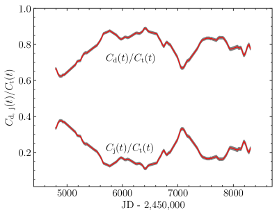
Figure 9: The ratio of the decomposed optical disk and jet flux to the total optical flux. Shaded areas represent the uncertainties.

4.4 Results

4.4.1 Overview

Figures 6 and 7 show the one- and two-dimensional distributions of the free parameters. The contours are plotted at $1\sigma$, $1.5\sigma$, and $2\sigma$ levels. Table 3 summarizes the best estimated parameter values determined from the medians of the posterior probability distributions and uncertainties determined from the 68.3% confidence intervals. The time delay of the H$\beta$ light curve with respect to the $V$-band light curve is $\tau_{\rm H\beta}=194.9_{-9.8}^{+9.7}$ days (in observed frame), slightly larger than $\tau_{\rm H\beta}=170.0_{-14.0}^{+9.6}$ days reported by Zhang et al. (2019), which used a linear fit to detrend the optical light curve. The time delay of the radio 15 GHz light curve with respect to the $V$-band light curve is $\tau_{\rm j}=501.0_{-10.2}^{+7.5}$ days. If regardless of the distance of the optical jet emission to the central black hole, the bulk of the 15 GHz emission is located at $c\tau_{\rm j}/(1+z)=0.36$ pc away from the black hole, where $c$ is the speed of light.

From Figure 7, we find that the averaged polarization degree of the jet emission at optical wavelengths is $\bar{p}_{\rm j}\approx 0.5\%$. This is consistent with the observed radio polarization $p\leqslant 1\%$ in the radio core of 3C 273 using the Very Long Baseline Array (Attridge 2001; Attridge et al. 2005; see also Hovatta et al. 2019). Such a low-level polarization in the core of the jet was generally ascribed to the differential Faraday depolarization. The averaged polarization angle is $\bar{\theta}_{\rm j}\approx 40^{\circ}$, which well agrees with the position angle ($\sim 42^{\circ}$) of the jet structure of 3C 273 (e.g., Roeser & Meisenheimer 1991). Such an alignment between polarization angle and jet structure axis was commonly observed in blazars (Rusk & Seaquist 1985; Impey et al. 1989; Blinov et al. 2020 and references therein).

In Figure 8, we plot best fits to the $V$-band, H$\beta$, and radio light curves. The decomposed disk and jet light curves at $V$-band are also superposed in the top panel of Figure 8. The $V$-band and radio light curves are well fitted. For the H$\beta$ light curve, although there are several detailed minor features (e.g., around JD 5250 and 8000) that cannot be reproduced, the main reconstructed variation patterns are in good agreement with observations. The discrepancies for these minor features may be ascribed to twofold reasons: 1) the assumed Gaussian transfer functions are simple so that the fitting is not expected to capture all the detailed features; 2) the 15 GHz radio emission of 3C 273 is core dominated, but there might be still a minor contamination from the large-scale jet (e.g., Perley & Meisenheimer 2017), which is not correlated with the optical jet emission. Nevertheless, as a zero-order approximation, our simple approach seems reasonable and enlightening.

For the sake of comparison, in the top panel of Figure 8, we also plot the linear polynomial used to detrend the continuum light curve by Zhang et al. (2019). Here, the polynomial is shifted vertically to align with the jet light curve. As can be seen, the slope of the polynomial is generally consistent with the declining trend of the jet light curve, indicating the validity of our decomposition procedure.

Figure 9 plots the obtained ratio of the optical disk and jet emission to the total emissions as a function of time, namely, $C_{\rm j}(t)/C_{\rm t}(t)$. The jet contributes $\sim 10\%$ of the optical emission at the minimum and $\sim 40\%$ at the maximum. The best fits to the optical polarization degree, polarization angle, and the Stokes parameters $Q/I$ and $U/I$ are plotted in Figure 4. As illustrated in Equations (19-21), besides the interstellar polarization and the accretion disk’s polarization, there are two contributions to the observed polarization variability: one is from $C_{\rm j}(t)/C_{\rm t}(t)$ and the other is from the jet itself $p_{\rm j}(t)$ and $\theta_{j}(t)$. By a visual inspection to Figures 4 and 9, we can find the global variation structures in $C_{\rm j}(t)/C_{\rm t}(t)$ generally match these of the observed optical polarization degree (except in short timesscales). Considering the fact that the variation patterns of $C_{\rm j}(t)/C_{\rm t}(t)$ (if regardless of its mean) does not depend on $f_{q}$, $\bar{p}_{\rm j}$, and $\bar{\theta}_{\rm j}$, the consistence in the global variation structures reinforces our assumption that the global polarizations are mainly contributed from the ratio $C_{\rm j}(t)/C_{\rm t}(t)$. Therefore, it is approximately viable to use averaged polarization degree $\bar{p}_{\rm j}$ and angle $\bar{\theta}_{\rm j}$ to decompose the optical light curves. However, it is because of this assumption that we cannot reproduce all the detailed, rapid variability in polarizations within timescales of months. Adding time-dependent perturbations to $\bar{p}_{\rm j}$ and $\bar{\theta}_{\rm j}$ would better fit the rapid polarization variability, but does not change the results of our calculations.

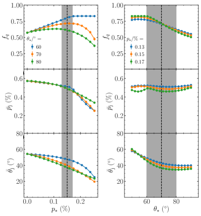
Figure 10: The best estimated values of $f_{q}$, $\bar{p}_{\rm j}$, and $\bar{\theta}_{\rm j}$ for different input interstellar (left) polarization degree $p_{\star}$ and (right) polarization angle $\theta_{\star}$. Dashed vertical lines represent the fiducial values $p_{\star}=0.15\%$ and $\theta_{\star}=70^{\circ}$. Shaded vertical bands represent the ranges between two previous observationally constrained interstellar polarization degree and angle ($p_{\star}=0.17\%$, $\theta_{\star}=80^{\circ}$) by Impey et al. (1989) and ($p_{\star}=0.13\%$, $\theta_{\star}=60^{\circ}$) by Smith et al. (1993).

Table 4: Inferred Values of $f_{q}$, $\bar{p}_{\rm j}$, and $\bar{\theta}_{\rm j}$ for different input interstellar polarization ($p_{\star},\theta_{\star}$).

$p_{\star}$	$\theta_{\star}$	$f_{q}$	$\bar{p}_{\rm j}$	$\bar{\theta}_{\rm j}$
(%)	(∘)		(%)	(∘)
0.13	60	$0.771_{-0.005}^{+0.005}$	$0.523_{-0.010}^{+0.010}$	$49.12_{-0.18}^{+0.19}$
0.13	80	$0.626_{-0.009}^{+0.007}$	$0.513_{-0.010}^{+0.009}$	$40.00_{-0.13}^{+0.13}$
0.17	60	$0.827_{-0.003}^{+0.002}$	$0.491_{-0.007}^{+0.006}$	$45.64_{-0.22}^{+0.24}$
0.17	80	$0.591_{-0.010}^{+0.009}$	$0.466_{-0.010}^{+0.010}$	$34.56_{-0.13}^{+0.13}$

4.4.2 The Influences of the Interstellar Polarization

In the above calculations, we fix the interstellar polarization degree $p_{\star}=0.15\%$ and polarization angle $\theta_{\star}=70^{\circ}$. In Figure 10, we show the dependence of the obtained $f_{q}$, $\bar{p}_{\rm j}$, and $\bar{\theta}_{\rm j}$ on the input interstellar polarization degree and angle. As described above, the previous observational constrains on the interstellar polarization along the direction of 3C 273 include ($p_{\star}=0.17\%$, $\theta_{\star}=80^{\circ}$) by Impey et al. (1989) and ($p_{\star}=0.13\%$, $\theta_{\star}=60^{\circ}$) by Smith et al. (1993). In Table 4, we list the resulting values of $f_{q}$, $\bar{p}_{\rm j}$, and $\bar{\theta}_{\rm j}$ for different pairs of the interstellar polarization ($p_{\star},\theta_{\star}$). By changing $p_{\star}$ from 0.13% to 0.17% with fixed $\theta_{\star}$, the influences on the obtained parameter values are minor. For $\theta_{\star}$ at a range of $(60^{\circ}-80^{\circ})$, the resulting $\bar{p}_{\rm j}$ almost has no change, while $f_{q}$ varies between $\sim$0.6 and $\sim$0.8 and $\bar{\theta}_{\rm j}$ varies between $\sim$35^∘ and $\sim$49^∘.

4.4.3 The Influences of Polarization of the Disk Emission

We by default neglect polarization of the disk emission in consideration of the nearly edge-on inclination ($i\sim 10^{\circ}$) of the accretion disk. To see how this affects the obtained parameters, we input different polarization degree $p_{\rm d}$ of the disk emission and show the results in Figure 11. Previous studies demonstrated that the polarization angle of the disk emission should be either parallel or perpendicular to the the symmetry axis of the scattering region (Goosmann & Gaskell 2007; Li et al. 2009), which is generally believed to align with the position angle of the jet. For 3C 273, the polarization angle of the disk emission is therefore either $42^{\circ}$ or $132^{\circ}$ (e.g., Roeser & Meisenheimer 1991). Meanwhile, if the polarization arises from scattering in equatorial torus, there might be a time delay between the polarized and the unpolarized disk emissions (Gaskell et al. 2012; Rojas Lobos et al. 2020). The size of the dust torus in 3C 273 inferred from near-infrared interferometry is about 960 days (Kishimoto et al. 2011). Thus, we also show the results for cases of the time delay fixed to $\tau_{\rm p}=960$ days in Figure 11. Regarding the parameter $f_{\rm q}$ that is directly related to our flux decomposition, the best estimated value increases with $p_{\rm d}$ for cases of $\theta_{\rm d}=42^{\circ}$ and approaches the upper limit of $f_{\rm q}\sim 0.83$ when $p_{\rm d}>0.06\%$. For cases of $\theta_{\rm d}=132^{\circ}$, the best estimated value of $f_{q}$ monotonously decreases with $p_{\rm d}$ and reaches $f_{q}\sim 0.55$ for a moderate value of $p_{\rm d}=0.1\%$. The best estimate of $f_{q}$ is insensitive to $\tau_{\rm p}$. As mentioned above, the disk emission with an inclination of $\sim 10^{\circ}$ generally has a very low degree of polarization because of symmetry. For example, the polarization degree of an optically thick disk is $\lesssim 0.05\%$ (Chandrasekhar, 1960, Section X). We therefore expect a reasonable range of $f_{q}\sim(0.6-0.8)$.

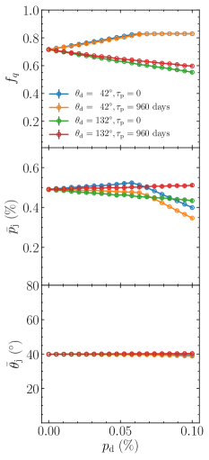
Figure 11: The best estimated values of $f_{q}$, $\bar{p}_{\rm j}$, and $\bar{\theta}_{\rm j}$ for different input polarization degree of disk emission. Differently colored points represent different input polarization angle $\theta_{\rm d}$ of the disk emission and the time delay $\tau_{\rm p}$ of the disk’s polarized emission with respect to the unpolarized emission.

5 Discussions

5.1 The Radio Light Curve

There are several programs that monitored 3C 273 at radio bands (e.g., Aller et al. 1999; Lister et al. 2009; Richards et al. 2011). We use the 15 GHz radio monitoring data from the Owens Valley Radio Observatory (Richards et al. 2011), which has the best sampling rate. According to the jet model developed by Türler et al. (1999), the variability of jet emissions arises from a series of synchrotron outbursts. Each burst produces a light curve with a rapid rise and slow decay with time (see Figure 1 in Türler et al. 1999). The synchrotron turnover frequency decreases as the shock front propagates along the jet. The resulting light curve from this model has a larger variability at higher frequency (Türler et al. 2000). This means that the flux correlations between different frequencies may be not simply linear and the relation between the radio and optical fluxes in Equation (6) should be regarded as a zero-order approximation.

Meanwhile, at low radio frequency the outer jet and its terminal hot spot may contribute mildly to the observed flux densities (e.g., Bahcall et al. 1995; Conway et al. 1993; Perley & Meisenheimer 2017). Therefore, it would be better to apply high-frequency radio light curves with sufficiently good sampling rate and long monitoring period in future once available.

5.2 The Damped Random Walk Model

We use the damped random walk model to describe the variability of the jet and disk emissions, which has been widely applied to AGN light curves (e.g., Kelly et al. 2009; Zu et al. 2011; Li et al. 2013, 2018; Pancoast et al. 2014). However, there was evidence from the Kepler observations that AGN light curves no longer obey the damped random walk model on short timescales less than days (Kasliwal et al. 2015). A more generic model would be the continuous-time autoregressive moving average (CARMA) model (Kelly et al. 2014; Takata et al. 2018), which can be regarded as a mixture of damped random walk models with different parameters. It is possible to incorporate the CARMA model in our framework, but at the expense of massive computational overheads. Indeed, different models mainly affect the short-timescale variability of the reconstructed light curves between measurement points. The high sampling of our compiled light curve data helps to minimize this influence. Moreover, the convolution operations in Equations (6) and (7) will also smooth the short-timescale variations to some extent. We therefore expect that the main results do not depend on the details of the adopted variability model.

5.3 The Gaussian Transfer Functions

For the sake of simplicity, we assume that both the transfer functions for the jet in Equation (6) and the broad-line region in Equation (7) are a single Gaussian. As such, all the covariance functions (see Appendix B) can be expressed analytically, which facilitates the calculations. There are two approaches for future improvements in practice. First, using multiple Gaussians to model the real transfer functions (Li et al. 2016). This will retain the advantage that the covariance functions have analytical forms. Second, employing a physical jet model and broad-line model to directly calculate the transfer functions. In particular for the broad-line region, there is a generic dynamical modeling method that works well for reverberation mapping data (Pancoast et al. 2014; Li et al. 2013, 2018). We expect that these two improvements could be beneficial to better fit the fine features in the light curves (in particular the H$\beta$ light curve), however, the main results of the present calculations should be retained.

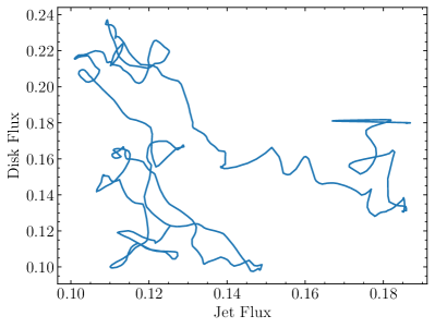
Figure 12: The relation between the decomposed disk emission $C_{\rm d}(t)$ and jet emission $C_{\rm j}(t)$.

5.4 The Accretion Disk-Jet Relation

In Figure 12, we plot the relation between the decomposed disk emission $C_{\rm d}(t)$ and jet emission $C_{\rm j}(t)$. The evolutionary track is fully random, consistent with our assumption that $C_{\rm d}(t)$ and $C_{\rm j}(t)$ are independent. This reinforces that the variability of the disk and jet is stochastic and independent at short timescales, even though they maybe eventually connected over the lifetime of the black hole activity (far much longer than the temporal baseline of the present data and our results are therefore not affected). Meanwhile, such stochastic variability of individual objects will contribute to the intrinsic scattering of the so-called fundamental plane of black hole activity (e.g., Merloni et al. 2003).

5.5 Implications for Reverberation Mapping Analysis

The phenomenon that optical continuum emissions show long-term trends that do not have a corresponding echo in line emissions is also incidentally detected in the past reverberation mapping campaigns (e.g., Welsh 1999; Denney et al. 2010; Li et al. 2013). A conventional procedure that detrends the light curves of emission lines and continuum with low-order polynomials was usually used to remove the induced biases in cross-correlation analysis (Denney et al. 2010; Peterson et al. 2014). For the campaign of 3C 273 reported in Zhang et al. (2019), if without detrending, the cross-correlation analysis on the light curves of the H$\beta$ line and the 5100 Å continuum yields a time lag as large as 298 days (in observed frame) and a maximum correlation coefficient of $r_{\rm max}=0.7$. After detrending the light curve of the 5100 Å continuum with a linear polynomial, the maximum correlation coefficient increases to $r_{\rm max}=0.8$ and the time lag turns to be 170 days (Zhang et al. 2019). The improvement on the maximum correlation coefficient illustrates that the detrending manipulation is necessary and worthwhile. Our work further reinforces such a detrending manipulation, however, the low-order polynomial should only be regarded as an approximation to the real trend. Indeed, we obtain a time lag of 194.9 days, larger by a factor of $\sim 15$% compared to the lag determined with the linear detrending by Zhang et al. (2019). Like the case of 3C 273, multi-wavelength monitoring data are highly required to reveal the origin of non-echoed trends and therefore to conduct realistic, physical detrending.

On the other hand, the presence of non-echoed trends means that there exists a non-negligible component of continuum emissions not involved in photoionization of the broad-line region. As a result, this component of emissions needs to be excluded when positioning the objects in the size-luminosity scaling relation of broad-line regions. For 3C 273, the mean 5100 Å flux is $19.46\times 10^{-15}~{}{\rm erg~{}s^{-1}~{}cm^{-2}~{}\text{\AA}^{-1}}$ (Zhang et al. 2019), corresponding a luminosity of $\log(\lambda L_{\lambda}/{\rm erg~{}s^{-1}})=45.86$ at 5100 Å with a luminosity distance of 787 Mpc. Once excluding a mean fraction $(1-f_{q})=0.284$ of the jet contribution, the realistic luminosity is changed to be $\log(\lambda L_{\lambda}/{\rm erg~{}s^{-1}})=45.72$, decreasing by about 0.14 dex. Accordingly, the dimensionless accretion rate $\mathscr{\dot{M}}=\dot{M}c^{2}/L_{\rm Edd}\propto(\lambda L_{\lambda})^{3/2}$ (e.g. Du et al. 2014) will decreases by about 0.2 dex, where $\dot{M}$ is the mass accretion rate and $L_{\rm Edd}$ is the Eddington luminosity. This implies that for objects similar to 3C 273, it is important to correct for the jet or otherwise contaminations when applying the size-luminosity scaling relation.

6 Conclusion

3C 273 is a flat-spectrum radio quasar with both a blue bump and a beamed jet. The recent reverberation mapping campaign reported by Zhang et al. (2019) showed that the optical continuum emissions display a non-echoed long-term trend compared to the emissions of the broad lines (such as H$\beta$ and Fe II). In this work, we compile multi-wavelength monitoring data of 3C 273 from the Swift archive and other ground-based programs at optical and radio wavelengths (including the the reverberation mapping campaign). The long-term trend of the Swift UV light curve is consistent with that of the H$\beta$ light curve but is clearly distinct from that of the optical light curves, exclusively indicating that there are two independent components of emissions at optical wavelength (see Section 3.1). This is further reinforced by the complicated color variation behaviours and the low-level optical polarizations of 3C 273 (see Sections 3.2 and 3.3). Considering the coexistence of the comparably prominent jet and blue bump in 3C 273, these lines of observations pinpoint to two-fold origins of the optical emissions: one is the accretion disk itself and the other is the jet.

We developed an approach to decouple the optical emissions from the jet and accretion disk using the reverberation mapping data, 15 GHz radio monitoring data, and optical polarization data. We implicitly assume that the 15 GHz radio emission represents an blurred echo of the jet emission at optical wavelength with a time delay. The results show that the jet emissions can well explain the non-echoed long-term trend in the optical continuum (in terms of the H$\beta$ reverberation mapping). In consideration of the low inclination angle ($\sim 10^{\circ}$) of the jet of 3C 273, we also simply assume that the disk emission has a negligible polarization. As a result, the jet quantitatively contributes a fraction of $\sim$10% at the minimum and up to $\sim$40% at the maximum to the total optical emissions. To our knowledge, this is the first time to interpret the conventional detrending procedure in reverberation mapping analysis with a physical process. Our work generally supports the procedure in which low-order polynomials are adopted to detrend the light curves, however, we bear in mind the limited practicability of such low-order polynomials. To conduct realistic detrending, one generally needs multi-wavelength monitoring data, especially UV data. Meanwhile, our work also implies that when applying the size-luminosity scaling relation for broad-line regions, one needs to carefully correct for the contaminations arising from non-echoed trends to optical luminosities. This is particularly important for objects similar to 3C 273 with both prominent jet and disk emissions.

Appendix A Reduction for the Swift Data

We used the HEASARC data archive to search for previous Swift observations of 3C 273 and download the data. We found 322 observations between 2004-12-13 and 2019-04-09, including 312 observations with exposures in both the X-ray Telescope (XRT) and the Ultraviolet/Optical Telescope (UVOT). We followed the standard threads and used HEAsoft (v6.25, Blackburn 1995) to reduce the data. Firstly the xrtpipeline script was used to reprocess the data with the latest calibration files. Then for each observation the uvotimsum script was used to sum all exposures in every filter. Observations in the UVOT grism mode were excluded because we only wanted to use the six UVOT photometric bands (i.e. UVW2, UVM2, UVW1, $U$, $B$, $V$). Then a circular aperture with a radius of 5 arcsec was used to enclose the source region, while the background was extracted from a nearby circular region with a radius of 20 arcsec without any point source. The uvotsource script was used to determine the magnitude and flux in every filter. We also ran the small-scale sensitivity check to identify data points affected by the lower throughput areas on the detector and discarded them. The final number of observations in every filter is listed in Table 1 (not every observation had exposures in all six UVOT filters). Note that 3C 273 appears slightly extended in all six UVOT filters, and so the absolute source fluxes comprise both the AGN emission and part of the host galaxy star-light which we did not subtract, but the variability of the source flux should be attributed to the central AGN activity. We tabulated our reduced Swift UVOT fluxes of 3C 273 in Table 5, in which only a portion of the data is shown and the entire table is available in a machine-readable form online.

Appendix B Covariance Functions

This appendix shows analytical expressions for the covariance functions in Section 4. The covariance function between $C_{\rm t}(t)$ and $L_{\rm H\beta}(t)$ is

$$S_{\rm tl}(\Delta t)=\langle C_{\rm t}(t_{k})L_{\rm H\beta}(t_{m})\rangle=\int\langle C_{\rm d}(t_{k})C_{\rm d}(t_{m})\rangle\Psi_{\rm H\beta}(t_{m}-\tau)d\tau,$$ (B1)

where $\Delta t=t_{m}-t_{k}$. With Equations (8) and (11), $S_{\rm tr}(\Delta t)$ has an analytical expression (see Li et al. 2016 for a detailed derivation)

$$S_{\rm tl}(\Delta t)=\frac{1}{2}\sigma_{\rm d}^{2}f_{\rm H\beta}e^{\omega_{\rm H\beta}^{2}/2T_{\rm d}^{2}}\left\{e^{-\Delta T/T_{\rm d}}{\rm erfc}\left[-\frac{1}{\sqrt{2}}\left(\frac{\Delta T}{\omega_{\rm H\beta}}-\frac{\omega_{\rm H\beta}}{T_{\rm d}}\right)\right]+e^{\Delta T/T_{\rm d}}{\rm erfc}\left[\frac{1}{\sqrt{2}}\left(\frac{\Delta T}{\omega_{\rm H\beta}}+\frac{\omega_{\rm H\beta}}{T_{\rm d}}\right)\right]\right\},$$ (B2)

where $\Delta T=\Delta t-\tau_{\rm H\beta}$ and ${\rm erfc}(x)$ is the complementary error function. The auto-covariance function of $L_{\rm H\beta}(t)$ is given by

$$S_{\rm ll}(\Delta t)=\frac{1}{2}\sigma_{\rm d}^{2}f_{\rm H\beta}^{2}e^{\omega_{\rm H\beta}^{2}/T_{\rm d}^{2}}\left\{e^{-\Delta t/T_{\rm d}}{\rm erfc}\left[-\frac{\Delta t}{2\omega_{\rm H\beta}}+\frac{\omega_{\rm H\beta}}{T_{\rm d}}\right]+e^{\Delta t/T_{\rm d}}{\rm erfc}\left[\frac{\Delta t}{2\omega_{\rm H\beta}}+\frac{\omega_{\rm H\beta}}{T_{\rm d}}\right]\right\}.$$ (B3)

The covariance function $S_{\rm tr}(\Delta t)$ between $C_{\rm t}(t)$ and $R_{\rm j}(t)$ and the auto-covariance function $S_{\rm rr}(\Delta t)$ of $R_{\rm j}(t)$ can be expressed in similar forms by replacing the subscript “$\rm H\beta$” and “d” with “j” in Equations (B2) and (B3).

Table 5: Swift UVOT data of 3C 273.

JD	UVW2	UVM2	UVW1	$U$	$B$	$V$
($+$2,450,000)	($10^{-14}~{}\rm erg~{}s^{-1}~{}cm^{-2}~{}\text{\AA}^{-1}$)
3562.086	$\cdots$	$\cdots$	$\cdots$	$8.452\pm 0.223$	$4.982\pm 0.095$	$3.341\pm 0.073$
3562.152	$19.011\pm 0.548$	$15.750\pm 0.349$	$13.219\pm 0.477$	$\cdots$	$\cdots$	$\cdots$
3689.602	$21.013\pm 0.607$	$17.487\pm 0.386$	$14.281\pm 0.518$	$6.147\pm 6.246$	$4.378\pm 0.092$	$3.403\pm 0.076$
3692.082	$21.157\pm 0.627$	$\cdots$	$\cdots$	$\cdots$	$\cdots$	$3.394\pm 0.102$
3721.746	$20.954\pm 0.608$	$17.682\pm 0.394$	$14.491\pm 0.528$	$6.208\pm 6.252$	$4.871\pm 0.104$	$3.550\pm 0.080$
$\cdots$

Note. — This table is available in its entirety in a machine-readable form in the online journal. Only a portion is shown here to illustrate its form and content.

References

- Abraham, & Romero (1999) Abraham, Z., & Romero, G. E. 1999, A&A, 344, 61
- Agol & Blaes (1996) Agol, E., & Blaes, O. 1996, MNRAS, 282, 965
- Aller et al. (1999) Aller, M. F., Aller, H. D., Hughes, P. A., & Latimer, G. E. 1999, ApJ, 512, 601
- Attridge (2001) Attridge, J. M. 2001, ApJ, 553, 31
- Attridge et al. (2005) Attridge, J. M., Wardle, J. F. C., & Homan, D. C. 2005, ApJ, 633, 85
- Bahcall et al. (1995) Bahcall, J. N., Kirhakos, S., Schneider, D. P., et al. 1995, ApJ, 452, L91
- Beloborodov (1998) Beloborodov, A. M. 1998, ApJ, 496, L105
- Bentz et al. (2013) Bentz, M. C., Denney, K. D., Grier, C. J., et al. 2013, ApJ, 767, 149
- Berriman et al. (1990) Berriman, G., Schmidt, G. D., West, S. C., et al. 1990, ApJS, 74, 869
- Bian et al. (2012) Bian, W.-H., Zhang, L., Green, R., et al. 2012, ApJ, 759, 88
- Blackburn (1995) Blackburn, J. K. 1995, in ASP Conf. Ser., Vol. 77, Astronomical Data Analysis Software and Systems IV, ed. R. A. Shaw, H. E. Payne, and J. J. E. Hayes (San Francisco: ASP), 367
- Blinov et al. (2020) Blinov, D., Casadio, C., Mandarakas, N., et al. 2020, A&A, 635, A102
- Bonning et al. (2012) Bonning, E., Urry, C. M., Bailyn, C., et al. 2012, ApJ, 756, 13
- Brewer et al. (2011) Brewer B. J., Páatay L. B, & Csányi G. 2011, Stat. Comput., 21, 649
- Brindle et al. (1990) Brindle, C., Hough, J. H., Bailey, J. A., et al. 1990, MNRAS, 244, 577
- Chandrasekhar (1960) Chandrasekhar, S. 1960, Radiative Transfer (New York: Dover)
- Chidiac et al. (2016) Chidiac, C., Rani, B., Krichbaum, T. P., et al. 2016, A&A, 590, A61
- Conway et al. (1993) Conway, R. G., Garrington, S. T., Perley, R. A., et al. 1993, A&A, 267, 347
- Courvoisier (1998) Courvoisier, T. J.-L. 1998, A&A Rev., 9, 1
- Denney et al. (2010) Denney, K. D., Peterson, B. M., Pogge, R. W., et al. 2010, ApJ, 721, 715
- Dai et al. (2009) Dai, B. Z., Li, X. H., Liu, Z. M., et al. 2009, MNRAS, 392, 1181
- Davis et al. (1991) Davis, R. J., Unwin, S. C., & Muxlow, T. W. B. 1991, Nature, 354, 374
- Drake et al. (2009) Drake, A. J., Djorgovski, S. G., Mahabal, A., et al. 2009, ApJ, 696, 870
- Du et al. (2014) Du, P., Hu, C., Lu, K.-X., et al. 2014, ApJ, 782, 45
- Du et al. (2016) Du, P., Lu, K.-X., Zhang, Z.-X., et al. 2016, ApJ, 825, 126
- Edelson et al. (2019) Edelson, R., Gelbord, J., Cackett, E., et al. 2019, ApJ, 870, 123
- Edelson et al. (2015) Edelson, R., Gelbord, J. M., Horne, K., et al. 2015, ApJ, 806, 129
- Fan et al. (2014) Fan, J. H., Kurtanidze, O., Liu, Y., et al. 2014, ApJS, 213, 26
- Foreman-Mackey (2016) Foreman-Mackey D., 2016, Journal of Open Source Software, 1, 24
- Gaskell et al. (2012) Gaskell, C. M., Goosmann, R. W., Merkulova, N. I., et al. 2012, ApJ, 749, 148
- Goosmann & Gaskell (2007) Goosmann, R. W., & Gaskell, C. M. 2007, A&A, 465, 129
- Grandi & Palumbo (2004) Grandi, P., & Palumbo, G. G. C. 2004, Science, 306, 998
- Gu et al. (2006) Gu, M. F., Lee, C.-U., Pak, S., et al. 2006, A&A, 450, 39
- Guo & Gu (2016) Guo, H., & Gu, M. 2016, ApJ, 822, 26
- Hazard et al. (2018) Hazard, C., Jauncey, D., Goss, W. M., & Herald, D. 2018, PASA, 35, e006
- Hovatta et al. (2019) Hovatta, T., O’Sullivan, S., Martí-Vidal, I., et al. 2019, A&A, 623, A111
- Hutsemékers et al. (2018) Hutsemékers, D., Borguet, B., Sluse, D., et al. 2018, A&A, 620, A68
- Ikejiri et al. (2011) Ikejiri, Y., Uemura, M., Sasada, M., et al. 2011, PASJ, 63, 639
- Impey et al. (1989) Impey, C. D., Malkan, M. A., & Tapia, S. 1989, ApJ, 347, 96
- Johnson (1966) Johnson, H. L. 1966, ARA&A, 4, 193
- Jorstad et al. (2017) Jorstad, S. G., Marscher, A. P., Morozova, D. A., et al. 2017, ApJ, 846, 98
- Kasliwal et al. (2015) Kasliwal, V. P., Vogeley, M. S., & Richards, G. T. 2015, MNRAS, 451, 4328
- Kaspi et al. (2000) Kaspi, S., Smith, P. S., Netzer, H., et al. 2000, ApJ, 533, 631
- Kelly et al. (2009) Kelly, B. C., Bechtold, J., & Siemiginowska, A. 2009, ApJ, 698, 895
- Kelly et al. (2014) Kelly, B. C., Becker, A. C., Sobolewska, M., et al. 2014, ApJ, 788, 33
- Kishimoto et al. (2011) Kishimoto, M., Hönig, S. F., Antonucci, R., et al. 2011, A&A, 527, 121
- Kochanek et al. (2017) Kochanek, C. S., Shappee, B. J., Stanek, K. Z., et al. 2017, PASP, 129, 104502
- Kriss et al. (1999) Kriss, G. A., Davidsen, A. F., Zheng, W., et al. 1999, ApJ, 527, 683
- Li et al. (2009) Li, L.-X., Narayan, R., & McClintock, J. E. 2009, ApJ, 691, 847
- Li et al. (2018) Li, Y.-R., Songsheng, Y.-Y., Qiu, J., et al. 2018, ApJ, 869, 137
- Li et al. (2016) Li, Y.-R., Wang, J.-M., & Bai, J.-M. 2016, ApJ, 831, 206
- Li et al. (2014) Li, Y.-R., Wang, J.-M., Hu, C., Du, P., & Bai, J.-M. 2014, ApJ, 786, L6
- Li et al. (2013) Li, Y.-R., Wang, J.-M., Ho, L. C., Du, P., & Bai, J.-M. 2013, ApJ, 779, 110
- Lister et al. (2009) Lister, M. L., Cohen, M. H., Homan, D. C., et al. 2009, AJ, 138, 1874
- Lister, & Smith (2000) Lister, M. L., & Smith, P. S. 2000, ApJ, 541, 66
- Malkan, & Sargent (1982) Malkan, M. A., & Sargent, W. L. W. 1982, ApJ, 254, 22
- Marin (2014) Marin, F. 2014, MNRAS, 441, 551
- Marscher & Gear (1985) Marscher, A. P., & Gear, W. K. 1985, ApJ, 298, 114
- Martini (2004) Martini, P. 2004, Coevolution of Black Holes and Galaxies, 169
- Merloni et al. (2003) Merloni, A., Heinz, S., & di Matteo, T. 2003, MNRAS, 345, 1057
- Paltani et al. (1998) Paltani, S., Courvoisier, T. J.-L., & Walter, R. 1998, A&A, 340, 47
- Pancoast et al. (2014) Pancoast, A., Brewer, B. J., & Treu, T. 2014, MNRAS, 445, 3055
- Perley & Meisenheimer (2017) Perley, R. A., & Meisenheimer, K. 2017, A&A, 601, A35
- Peterson (1993) Peterson, B. M. 1993, PASP, 105, 247
- Peterson et al. (2014) Peterson, B. M., Grier, C. J., Horne, K., et al. 2014, ApJ, 795, 149
- Peterson et al. (1995) Peterson, B. M., Pogge, R. W., Wanders, I., et al. 1995, PASP, 107, 579
- Phillips & Meszaros (1986) Phillips, K. C., & Meszaros, P. 1986, ApJ, 310, 284
- Planck Collaboration et al. (2014) Planck Collaboration, Ade, P. A. R., Aghanim, N., et al. 2014, A&A, 571, A21
- Plavin et al. (2019) Plavin, A. V., Kovalev, Y. Y., & Petrov, L. Y. 2019, ApJ, 871, 143
- Rani et al. (2010) Rani, B., Gupta, A. C., Strigachev, A., et al. 2010, MNRAS, 404, 1992
- Richards et al. (2011) Richards, J. L., Max-Moerbeck, W., Pavlidou, V., et al. 2011, ApJS, 194, 29
- Rojas Lobos et al. (2020) Rojas Lobos, P. A., Goosmann, R. W., Hameury, J. M., et al. 2020, A&A in press, arXiv:2004.03957
- Rojas Lobos et al. (2018) Rojas Lobos, P. A., Goosmann, R. W., Marin, F., et al. 2018, A&A, 611, A39
- Roeser & Meisenheimer (1991) Roeser, H.-J., & Meisenheimer, K. 1991, A&A, 252, 458
- Ruan et al. (2014) Ruan, J. J., Anderson, S. F., Dexter, J., et al. 2014, ApJ, 783, 105
- Rudy et al. (1983) Rudy, R. J., Schmidt, G. D., Stockman, H. S., et al. 1983, ApJ, 271, 59
- Rusk & Seaquist (1985) Rusk, R., & Seaquist, E. R. 1985, AJ, 90, 30
- Rybicki & Press (1992) Rybicki, G. B., & Press, W. H. 1992, ApJ, 398, 169
- Savolainen et al. (2006) Savolainen, T., Wiik, K., Valtaoja, E., et al. 2006, A&A, 446, 71
- Schmidt et al. (2012) Schmidt, K. B., Rix, H.-W., Shields, J. C., et al. 2012, ApJ, 744, 147
- Shappee et al. (2014) Shappee, B. J., Prieto, J. L., Grupe, D., et al. 2014, ApJ, 788, 48
- Simmons & Stewart (1985) Simmons, J. F. L., & Stewart, B. G. 1985, A&A, 142, 100
- Smith et al. (2002) Smith, J. E., Young, S., Robinson, A., et al. 2002, MNRAS, 335, 773
- Smith et al. (2009) Smith, P. S., Montiel, E., Rightley, S., et al. 2009, arXiv:0912.3621
- Smith et al. (1993) Smith, P. S., Schmidt, G. D., & Allen, R. G. 1993, ApJ, 409, 604
- Soldi et al. (2008) Soldi, S., Türler, M., Paltani, S., et al. 2008, A&A, 486, 411
- Stevens et al. (1998) Stevens, J. A., Robson, E. I., Gear, W. K., et al. 1998, ApJ, 502, 182
- Stockman et al. (1984) Stockman, H. S., Moore, R. L., & Angel, J. R. P. 1984, ApJ, 279, 485
- Takata et al. (2018) Takata, T., Mukuta, Y., & Mizumoto, Y. 2018, ApJ, 869, 178
- Türler et al. (2006) Türler, M., Chernyakova, M., Courvoisier, T. J.-L., et al. 2006, A&A, 451, L1
- Türler et al. (2000) Türler, M., Courvoisier, T. J.-L., & Paltani, S. 2000, A&A, 361, 850
- Türler et al. (1999) Türler, M., Paltani, S., Courvoisier, T. J.-L., et al. 1999, A&AS, 134, 89
- Wang et al. (2020) Wang, J.-M., Songsheng, Y.-Y., Li, Y.-R., et al. 2020, Nature Astronomy, 9
- Welsh (1999) Welsh, W. F. 1999, PASP, 111, 1347
- Wolf & Henning (1999) Wolf, S., & Henning, T. 1999, A&A, 341, 675
- Wu (1977) Wu, C.-C. 1977, ApJ, 217, L117
- Xiong et al. (2017) Xiong, D., Bai, J., Zhang, H., et al. 2017, ApJS, 229, 21
- Zeng et al. (2018) Zeng, W., Zhao, Q.-J., Dai, B.-Z., et al. 2018, PASP, 130, 024102
- Zhang et al. (2019) Zhang, Z.-X., Du, P., Smith, P. S., et al. 2019, ApJ, 876, 49
- Zu et al. (2011) Zu, Y., Kochanek, C. S., & Peterson, B. M. 2011, ApJ, 735, 80