PySPH: a Python-based framework for smoothed particle hydrodynamics

Abstract.

PySPH is an open-source, Python-based, framework for particle methods in general and Smoothed Particle Hydrodynamics (SPH) in particular. PySPH allows a user to define a complete SPH simulation using pure Python. High-performance code is generated from this high-level Python code and executed on either multiple cores, or on GPUs, seamlessly. It also supports distributed execution using MPI. PySPH supports a wide variety of SPH schemes and formulations. These include, incompressible and compressible fluid flow, elastic dynamics, rigid body dynamics, shallow water equations, and other problems. PySPH supports a variety of boundary conditions including mirror, periodic, solid wall, and inlet/outlet boundary conditions. The package is written to facilitate reuse and reproducibility. This paper discusses the overall design of PySPH and demonstrates many of its features. Several example results are shown to demonstrate the range of features that PySPH provides.

1. Introduction

Particle methods are a class of numerical methods where particles are used to carry physical properties. These properties evolve as per the governing differential equations of the problem. They may be used to simulate continuum mechanics problems which is our present interest. Particle methods are typically Lagrangian and meshless and this allows the method to handle problems with free-surfaces and large deformations. The Smoothed Particle Hydrodynamics method (SPH) was independently developed by Lucy (1977) and Gingold and Monaghan (1977). The method has since developed to simulate a wide variety of problems in continuum mechanics.

A typical meshless particle method implementation requires the following,

• representation of the field properties in terms of particles.

• reconstruction of the field properties and their derivatives using the particle positions and properties alone.

• identification of neighboring particles.

• evolution of the particle properties over time.

There are various open-source software packages like DualSphysics (Crespo et al., 2015), GADGET-4 (Springel et al., 2020), AquaGPUSph (Cercos-Pita, 2015), PHANTOM (Price et al., 2018), SPlisHSPlasH (Koschier et al., 2019) among others which solve SPH problems efficiently. A fairly exhaustive listing of open source and commercial packages is provided in the review by Shadloo et al. (2016). In Table 1 many open source SPH packages and their features are listed. The footnotes explain the respective columns.

	MPI/GPU	Language	NNPS	CI	Docs	Notes
AQUAGPUsph (Cercos-Pita, 2015)	MPI & GPU	C++	Cell-grid	No	No	WCSPH
DualSPHysics (Crespo et al., 2015)	GPU	C++	Cell-grid	No	Yes	WCSPH, Elastic, DEM
GADGET4 (Springel et al., 2020)	MPI	C++	Octree	No	Yes	Compressible, Astrophysics
GIZMO (Hopkins, 2015)	MPI	C	Octree	No	Yes	Compressible, Astrophysics
GPUSPH (Bilotta et al., 2016)	MPI & GPU	C++	Cell-grid	No	Yes	WCSPH
PHANTOM (Price et al., 2018)	MPI	FORTRAN	Octree	Yes	Yes	Compressible, Astrophysics
PySPH	MPI & GPU	Python	Cell-grid, Octree	Yes	Yes	WCSPH, ISPH, Compressible, Elastic, DEM
SPHERA (Amicarelli et al., 2020)	No	FORTRAN	Cell-grid	No	No	WCSPH
SPHERAL++ (Owen et al., 11)	MPI	C++/Python	Octree	No	No	WCSPH, Compressible, Astrophysics, Elastic
SPHinXsys (Zhang et al., 2020)	No	C++	Cell-grid	No	Yes	WCSPH, Elastic
SPlisHSPlasH (Koschier et al., 2019)	MPI & GPU	C++/Python	Cell-grid	No	No	WCSPH, ISPH, Elastic

Table 1. The summary of packages available for particle methods.

From the Table 1 it can be seen that all of these packages (except PySPH) are implemented in a lower-level programming language like C, C++, or FORTRAN. While some of these feature a Python interface, the primary programming language used to implement the schemes is still in a lower-level language. One can also see that apart from the PHANTOM package, the other packages do not employ any form of continuous integration testing that is public. Studies (Prechelt, 2000; Gmys et al., 2020) have indicated that higher-level programming languages like Python (van Rossum et al., 91) lead to more programmer productivity. Python is also acknowledged by these studies and other articles (Perkel, 2015) as a popular language and as a good introductory programming language (Guo, 2014). Our own experience has indicated that the use of a high-level language makes the code a lot more accessible to students and researchers. Python features extensive libraries for scientific computation, general purpose tasks, and easily interfaces with lower-level languages like C/C++, FORTRAN as well as OpenCL and CUDA. These reasons make it an ideal choice for use in PySPH.

Many of the existing SPH related packages are developed with a few particular SPH schemes or application domains in mind. For example, many of the packages mentioned above do not solve elastic dynamics and while some solve incompressible fluid mechanics problems they do not support compressible fluid flow and vice-versa. In addition, there are other meshless methods like the Discrete Element Method (DEM) (Cundall and Strack, 1979), Reproducing Kernel Particle Method (RKPM) (Liu et al., 1995), Moving Least-Squares Particle Hydrodynamics (MLSPH) (Dilts, 1999), and others (see (Nguyen et al., 2008) for a review of meshless methods). Researchers are continuing to explore new methods and techniques in order to improve their efficiency and accuracy. It is difficult to perform research in a new area without investing a significant amount of time in building the necessary tools. Our goal in creating PySPH is to make it possible for researchers to build upon the work of others with relative ease. To this end PySPH provides,

• data-structures to store particle properties irrespective of the meshless method being used.

• algorithms to find nearest neighbors of particles for various uses.

• the ability to write high-level Python code to express the inter-particle interactions and have them seamlessly execute on multi-core CPUs and GPUs.

• implementation in the form of reusable libraries. This is in contrast with tools that only seek to solve specific problems.

Furthermore, to promote usability, extensibility, and quality, PySPH

• is distributed under a liberal, open-source, BSD (three-clause) license. This does not restrict commercial use of the software.

• is a cross platform package that works on the major platforms today viz. Linux, Windows, and MacOS.

• is written using modern software engineering practices including public hosting on https://github.com/pypr/pysph, easily accessible documentation, the use of unit tests, and continuous integration testing.

• provides a large number of well established schemes.

• provides an extensive collection of reusable benchmark and example problems.

• uses a high-level and easy to read programming language, Python (van Rossum et al., 91).

In order to promote reproducible research, PySPH is relatively easy to install using standard tools available in the Python ecosystem. This allows researchers to share their relevant changes alone which in combination with PySPH can be used to reproduce results. PySPH seeks to offer these features without sacrificing computational performance. This is important since SPH simulations can be computationally demanding. PySPH therefore runs on multi-core CPUs, GPUs and also supports distributed execution on clusters. PySPH supports these without requiring any major changes to the user code. PySPH was originally designed to run in serial on CPUs and be distributed using MPI. In 2013 it was redesigned and reimplemented to make use of automatic code generation from high-level Python. This made PySPH much easier to use and also demonstrated improved performance. Some historical details and design decisions are mentioned in (Ramachandran, 2016).

PySPH uses object-orientation for maximum reuse and managing complexity. Python is used to specify the inter-particle interactions and high-performance code is generated from this high-level specification. Source templates are used to abstract any common patterns and generate code. These features allow for a great deal of flexibility without sacrificing much performance.

While PySPH has been used extensively by our group, it has been used in several recent papers by other researchers in the community (Meyer et al., 2020; Arai et al., 2020; Li et al., 2018; Bao et al., 2019).

The next section outlines the basic equations employed in SPH in order to provide a brief background. We then discuss the design of the PySPH framework by showing how one may solve a simple problem with it. We use this example to highlight the features and design of PySPH. We then show several sample applications from PySPH to benchmark and demonstrate its wide applicability. We also discuss the computational performance of PySPH.

2. The SPH method

In this section we briefly introduce the SPH method. We refer the reader to (Violeau, 2012) for a detailed discussion. SPH is a Lagrangian, meshless, particle method, where the particles represent the underlying continuum. In SPH, a field variable $f(\mathbf{x})$ over a domain $\Omega$ can be approximated by a convolution with the kernel function $W(\mathbf{x},h)$:

(1) $$f(\mathbf{x})=\int_{\Omega}f(\mathbf{y})W(\mathbf{x}-\mathbf{y},h)\text{d}\mathbf{y},$$

where $h$ is the smoothing length, and $\text{d}\mathbf{y}$ is the differential volume element. The kernel function approximates the delta function in the limit $h\rightarrow 0$ and is a compact function such that $W(\mathbf{r})=0$ when $|\mathbf{r}|>kh$ for some constant $k$. To obtain the discrete counterpart the field is discretized into particles having mass $m_{i}$, density $\rho_{i}$, and the differential volume is replaced by the volume $V_{i}=m_{i}/\rho_{i}$ where the subscript denotes the index of the $i^{th}$ particle at position $\mathbf{x}_{i}$. The integral is then approximated by a summation:

(2) $$f(\mathbf{x}_{i})=\sum_{j}V_{j}f(\mathbf{x}_{j})W(\mathbf{x}_{i}-\mathbf{x}_{j},h),$$

where the summation is over all the particle in the support of the kernel function. If the function $f(\mathbf{x}_{i})$ is replaced by density $\rho(\mathbf{x}_{i})$ we get the summation density formula in SPH,

(3) $$\rho(\mathbf{x}_{i})=\sum_{j}m_{j}W(\mathbf{x}_{i}-\mathbf{x}_{j},h).$$

The SPH approximation can be used to discretize partial differential equations. The governing equations of motion for a fluid flow, expressed in the Lagrangian form, are,

(4) $$\frac{d\rho}{dt}=-\rho\nabla\cdot\mathbf{u},$$

(5) $$\frac{d\mathbf{u}}{dt}=-\frac{1}{\rho}\nabla p+\nu\nabla^{2}\mathbf{u}+\mathbf{g},$$

where $\frac{d(.)}{dt}$ is the material derivative, $\rho$ is the density, $p$ is the pressure, $\nu$ is the kinematic viscosity, and $\mathbf{g}$ is the external acceleration. In the case of a weakly-compressible fluid, the equation of state which completes the above equations is,

(6) $$p=\frac{c^{2}_{0}\rho_{0}}{\gamma}\left[{\left(\frac{\rho}{\rho_{0}}\right)}^{\gamma}-1\right],$$

where $\gamma=7$, $\rho_{0}$ and $c_{0}$ is the reference density and speed of sound. In the case of a compressible fluid, the equations include an energy equation and a different equation of state. The discrete form of the above equations using SPH approximation can be written as,

(7) $$\frac{d\rho_{i}}{dt}=\sum_{j}m_{j}(\mathbf{v}_{i}-\mathbf{v}_{j})\cdot\nabla_{i}W_{ij},$$

(8) $$\frac{d\mathbf{u}_{i}}{dt}=\mathbf{a}_{\text{p}}+\mathbf{a}_{\text{visc}}+\mathbf{a}_{\text{body}},$$

where $\rho_{i}$, $\mathbf{u}_{i}$ is respectively the density and velocity of the $i^{\text{th}}$ particle. $\mathbf{a}_{\text{p}}$ is the acceleration due to pressure gradient commonly discretized (Monaghan, 1992) as,

(9) $$\mathbf{a}_{\text{p}}=-\sum_{j}m_{j}\left(\frac{p_{i}}{\rho_{i}^{2}}+\frac{p_{j}}{\rho_{j}^{2}}\right)\nabla_{i}W_{ij},$$

where $p_{i}$ is pressure of $i^{\text{th}}$ particle, $p_{j}$ is pressure, $m_{j}$ is the mass, and $\rho_{j}$ is the density of the $j^{\text{th}}$ particle, $\nabla_{i}W_{ij}=\frac{\partial W}{\partial\mathbf{x}_{i}}(\mathbf{x}_{i}-\mathbf{x}_{j},h)$ is the gradient of the smoothing kernel. $\mathbf{a}_{\text{visc}}$ is the acceleration due to viscous forces is (Monaghan, 2005),

(10) $$\mathbf{a}_{\text{visc}}=\sum_{j}m_{j}\frac{4\nu}{(\rho_{i}+\rho_{j})}\frac{\mathbf{r}_{ij}\cdot\nabla_{i}W_{ij}}{(|\mathbf{r}_{ij}|^{2}+\eta h^{2})}\mathbf{u}_{ij},$$

where $\mathbf{r}_{ij}=\mathbf{x}_{i}-\mathbf{x}_{j}$, and $\mathbf{a}_{\text{body}}$ is the acceleration due to external body forces. Finally, the particle positions are obtained by integrating in time the following ODE,

(11) $$\frac{d\mathbf{x}_{i}}{dt}=\mathbf{u}_{i}.$$

The problem we are going to consider in the next section is the simulation of a two-dimensional dam break (Gomez-Gesteria et al., 2010) where a column of fluid is placed in a tank and simulated under the influence of gravity. For the purpose of illustration we consider a simple treatment of the boundary conditions. The tank is represented by solid particles having the same mass as the fluid particles on which we solve the continuity equation and then set the pressure by using the equation of state equation (6).

2.1. Time Integration

The equations of motion and momentum equations are then integrated in time to obtain the positions and velocities respectively, a Predictor-Corrector integrator (Monaghan, 2005) is used to integrate in time which is described as,

(12) $$\mathbf{u}^{n+\frac{1}{2}}_{i}=\mathbf{u}^{n}_{i}+\frac{\Delta t}{2}{\left(\frac{d\mathbf{u}_{i}}{dt}\right)}^{n},$$

(13) $$\mathbf{x}^{n+1}_{i}=\mathbf{x}^{n}_{i}+\Delta t\mathbf{u}^{n+\frac{1}{2}}_{i},$$

(14) $$\mathbf{u}^{n+1}_{i}=\mathbf{u}^{n+\frac{1}{2}}_{i}+\frac{\Delta t}{2}{\left(\frac{d\mathbf{u}_{i}}{dt}\right)}^{n+1}.$$

The time-step for the integration is based on a CFL criterion that depends on the differential equations being solved. In the SPH literature, implicit time-stepping is not very common as a result PySPH does not currently support these. The issue of stiffness of the system is also not explicitly handled by PySPH. However, it is useful to note that PySPH does support iterative solution of matrices using a matrix-free formulation and this is discussed in a little more detail in section 3.4.1.

2.2. Nearest neighbor particle search

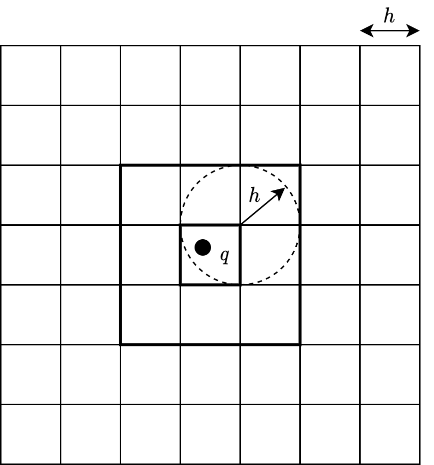
In order to find the particles that fall under the support of a kernel, a nearest neighbor particle searching (NNPS) algorithm is used. The uniform grid data structure is the most commonly used approach for NNPS. It works by dividing the particles into cells of size equal to the support radius. The neighbors of a particle are then searched in the neighboring $3^{d}$ boxes of the query particle as shown in figure 1, where $d$ is the number of dimensions. This method works efficiently when the support radius is constant for all particles, but when the support radius is variable, the cell size needs to be the maximum support radius which makes the uniform grid based approach inefficient as the cells become too large. To efficiently find neighbors in cases of variable support radius, a data structure with adaptive cell size needs to be used. The most common approach in these cases is to use an Octree (Hernquist and Katz, 1989; Springel, 2005). As part of PySPH, we provide the following algorithms for NNPS on the CPU:

• Spatial Hash. In this method, each cell in the uniform grid is mapped to an index in a hash table. Using a hash table allows storing of only the non-empty cells at the cost of a poor cache performance.

• Linked List (Dominguez et al., 2011). This method maps each cell to a flattened 1D cell ID which is mapped into a head array which stores the first particle of that cell. Another array next maps each particle to the next particle in that cell. This algorithm gives a better cache performance because of its compactness, but needs to allocate an array of size equal to the number of cells in the domain including the empty cells.

• Z-Order Space Filling Curve. Space filling curves are used to map 3D and 2D data to one-dimension while preserving spatial locality. A Z-Order SFC is constructed by sorting the particle IDs by keys that are generated using bit-interleaving (Morton, 1966). This method gives the best cache performance in uniform grids, but requires a sort in the build step which makes it slower overall than the linked list NNPS.

• Octree. In this method we recursively divide the space into 8 octants until a node has less than a specified number of particles. When querying neighbors, the tree is traversed in a top-down order and only the octants that intersect with the bounding box of the query region are traversed.

In addition to these, there are a few experimental NNPS algorithms implemented in PySPH which will be discussed in a later publication. Due to its highly parallel nature and a number of other restrictions, not all of the above algorithms can be efficiently implemented on a GPU. PySPH provides the Z-Order SFC, and the Octree algorithms for NNPS on the GPU.

Figure 1. Nearest neighbors of particle $q$ with support radius $h$ can be found in the 9 neighboring boxes of the cell that $q$ belongs to.

2.3. Schemes

The SPH method can be used to simulate a wide variety of problems. There are many schemes and variants of the basic scheme. The PySPH framework provides an implementation of many of these.

• In the weakly compressible SPH family, PySPH implements the classic scheme of (Monaghan, 1994), the corrections from (Hughes and Graham, 2010), the tensile instability correction (Monaghan, 2000), the $\delta$-SPH (Marrone et al., 2011) method, the Transport Velocity Formulation (TVF) (Adami et al., 2013), the Generalized TVF (GTVF) (Zhang et al., 2017), the Entropically Damped Artificial compressibility (EDAC) (Ramachandran and Puri, 2019), the Dual time SPH (DTSPH) (Ramachandran et al., 2019). Equations modeling surface tension (Morris, 2000; Adami et al., 2010) are also included in the framework.

• In the family of Incompressible SPH (ISPH) schemes, the projection method of (Cummins and Rudman, 1999), the Implicit ISPH (IISPH) (Ihmsen et al., 2014), the simple iterative ISPH (SISPH) (Muta et al., 2019).

• In the family of compressible SPH schemes, the Godunov SPH (GSPH) (Inutsuka, 2002), and the approximate Riemann solver with Godunov SPH (Puri and Ramachandran, 2014), the adaptive density kernel estimate (ADKE) method (Sigalotti et al., 2006), the Monaghan-Price-Morris (MPM) method (Price, 2012), and the conservative reproducible kernel SPH (Frontiere et al., 2017).

• For elastic dynamics PySPH implements the method of Gray-Monaghan (Gray et al., 2001), the Generalized TVF (GTVF) (Zhang et al., 2017), two way rigid-fluids coupling (Akinci et al., 2012) and rigid body dynamics.

• For the shallow water equations, PySPH implements the dynamic particle splitting and merging (Vacondio et al., 2013, 2012), Corrected SPH (CSPH) (Rodriguez-Paz and Bonet, 2005), and the Lax-Friedrichs flux based stabilization term (Riadh and Soulaïmani, 2005).

• Additional improvements and corrections that are available are the kernel and gradient corrections of (Bonet and Lok, 1999) and the shifting algorithms of (Xu et al., 2009; Skillen et al., 2013).

• Boundary conditions are also implemented in the framework which include, wall boundary conditions (Adami et al., 2012), inlet boundary conditions and various outlet boundary conditions which includes, Do nothing (Federico et al., 2012), Hybrid (Negi et al., 2020), Method of characteristics (Lastiwka et al., 2009), Mirror (Tafuni et al., 2018) boundary conditions.

We next discuss the implementation, usage and design of PySPH in considerable detail.

3. Implementation, usage, and design

PySPH may be installed using standard installation procedures available in the Python ecosystem. Documentation on this is available as part of the PySPH online documentation. The documentation is available at https://pysph.readthedocs.io and includes installation, tutorial, and reference material on PySPH.

3.1. Design overview

The overall design of PySPH can be broken down into the following pieces of infrastructure.

pysph.base:

provides utilities for the management of a large number of particles.

• The package provides a ParticleArray class which contains the functionality to create and remove particles, access and change their properties etc.

• The pysph.base package also implements many algorithms to find the nearest neighbors of particles in the vicinity of a given particle. These algorithms include ones for fixed and variable smoothing kernel radius as well as CPU and GPU algorithms as discussed in Section 2.2.

• The commonly used SPH kernels are also available in pysph.base.kernels.

pysph.sph:

provides functionality to write the low-level computations for SPH in pure Python. Internal functionality to convert the high-level Python code describing the SPH algorithms into high-performance code is provided here. This includes execution on multi-core CPUs and GPU architectures. The building blocks of many existing SPH formulations are also implemented in this package as Equations and Schemes which are discussed later.

pysph.solver:

provides the Application and Solver classes that combine the basic tools in the other packages to create easy-to-use command line applications that solve specific problems.

pysph.tools:

provides many general purpose miscellaneous tools for visualization, post-processing, input/output, etc.

pysph.parallel:

contains the code for distributed execution via MPI.

pysph.examples:

provides over 90 examples that simulate many benchmark problems. Some of these include post-processing and comparison with exact, experimental, and computational results. These examples are written in a way that they may be reused.

In order to perform the above efficiently, PySPH relies on general purpose functionality provided by the following sister packages.

• cyarray is a simple package that provides an interface to a typed C-like array. It also interfaces easily with NumPy (Oliphant, 2006) arrays.

• compyle allows a user to generate high-performance code from a restricted subset of pure Python. This can be used to write algorithms that use multi-core CPUs and GPUs efficiently but from the convenience of the Python programming language. More details are available in (Bhosale and Ramachandran, 2020).

• pyzoltan is a Python wrapper for the ZOLTAN(Boman et al., 1999, 2012) package. It is used to distribute the particles across multiple computers to scale up the computations (Puri et al., 2013).

These are currently separate packages but were originally part of the PySPH package. They are general purpose packages and may be used independently of PySPH.

3.2. An example problem

PySPH provides many low-level tools for a developer to create their own particle methods simulator. However, PySPH provides a high-level framework for the convenience of researchers whose focus is on the rapid implementation of an SPH code. In this section, this high-level framework is described. We look at a simple example problem and show how to implement this in PySPH. We then go over the details of how PySPH executes the resulting example internally.

We consider a simple dam-break problem in two dimensions with the standard weakly-compressible SPH formulation (Monaghan, 1994) whose equations are discussed in the earlier section. This example is available as part of the repository supporting this article, here. The file is about 125 lines of pure Python. We can immediately execute the example using the following:

$ python db2d.py

This will generate high-performance C++ code that runs on a single core of a CPU. As the simulation runs, output files are dumped into a db2d_output directory. The output files are in the form of NumPy NpzFiles or HDF5 files (if the package h5py is installed).

We may run the same code on all CPU cores with this invocation,

$ python db2d.py --openmp

Furthermore, if one has a GPU or OpenCL support, one can also invoke this as,

$ python db2d.py --opencl

If one is using MPI and has configured PySPH to use MPI, one may run this as,

$ mpirun -np 4 python db2d.py

No change to the code is needed. Although with the very few particles in this problem, it would be much slower to execute this on a GPU or on multiple CPUs with MPI. The ability for PySPH to execute the same unmodified Python code on different platforms efficiently is an important and powerful feature.

Thus, the Python file is really a specification for the SPH simulation and the framework takes care of generating the appropriate code. Since the code is Python, it promotes reuse and one may use the standard Python mechanisms for this.

The default application also supports many command line options, these may be seen by passing the --help option to the program which will print a help message with all command line options.

We now look at the details of how we implement this. The high-level PySPH framework employs an object-oriented design to minimize repetition and facilitate reuse. The first step in solving the dam-break problem is to create a new Application subclass that implements the necessary methods. We show an outline of such an example in the following listing 1.

Listing 1: Outline of 2d dam break example.

⬇

from pysph.solver.application import Application

class DamBreak2D(Application):

def create_particles(self):

# ...

def create_equations(self):

# ...

def create_solver(self):

# ...

if __name__ == ’__main__’:

app = DamBreak2D()

app.run()

The code in Listing 1 outlines the basic methods that one may overload to create an application. The important methods shown are the following:

• create_particles: where the user creates ParticleArray instances to represent the different physical entities as particles.

• create_equations: where the SPH equations are suitably grouped and instantiated. These equations typically implement the right-hand-side of the SPH discretized equations (7), (8).

• create_solver: where a Solver instance is suitably created. The solver manages an Integrator which in turn uses the generated equations to compute the acceleration terms.

We now show the details of the various methods. We begin with the creation of the particles.

3.2.1. Creation of particles

Listing 2: Implementation of the create_particles method.

⬇

import pysph.tools.geometry as G

from pysph.base.utils import get_particle_array_wcsph

class DamBreak2D(Application):

def create_particles(self):

dx, hdx, rho = 0.1, 1.2, 1000

xf, yf = G.get_2d_block(

dx=dx, length=1.0, height=2.0, center=[-1.5+dx, 1+dx]

)

m = dx**2 * rho

fluid = get_particle_array_wcsph(

name=’fluid’, x=xf, y=yf, h=hdx*dx, m=m, rho=rho

)

xt, yt = G.get_2d_tank(

dx=dx, length=4.0, height=4.0, num_layers=3

)

solid = get_particle_array_wcsph(

name=’solid’, x=xt, y=yt, h=hdx*dx, m=m, rho=rho

)

return [fluid, solid]

In the Listing 2, the code used to generate the geometry is shown. Here we make use of some functions provided in the pysph.tools.geometry module to create a tank and a block of particles. These functions return NumPy (Oliphant, 2006) arrays that define the particle positions. The fluid variable is a ParticleArray instance. The get_particle_array_wcsph method is merely a convenience that pre-defines several important default particle properties like the x, y, z, u, v, w, p which represent the position, velocity, and pressure. The property h is the smoothing length of the kernel and this parameter also determines the search radius for the NNPS when finding neighbors. It is important to note that all particle arrays should have a name that is a valid Python variable name. The solid particle array is also created similarly. The pysph.tools.geometry provides a few functions to create shapes used in standard benchmark problems in two and three dimensions. The geometry module has just been shown here for illustration and one may create the particles in any other way as a collection of points specified as NumPy arrays. Once the particle arrays are setup, they are returned from the create_particles method as a list. A ParticleArray manages a collection of properties and these are accessible in the manner shown in the following example:

⬇

>>> fluid.get_number_of_particles()

231

>>> fluid.x

array([-1.9, ..., -0.9])

>>> fluid.rho

array([1000., ..., 1000.])

Particle arrays allow us to operate on the entire collection of particles as a whole. This means that a property is something that has a potentially different value for each particle. One may add more properties using the fluid.add_property() method to the existing particle arrays. Each property illustrated in the code (x, y, u, v) has a single quantity per particle. For a vectorial or tensor quantities it is sometimes more convenient to associate 3 or 9 elements per particle as a single property. For these cases, particle arrays allow the specification of a “stride”. Hence for a vector quantity the stride would be set to 3. The data is still stored as a one-dimensional array but the user could use the stride when accessing the appropriate values.

Some properties like viscosity are constant for all the particles and can be added using fluid.add_constant(). In addition to this there are methods to add particles, remove particles, extract particles into another particle array etc. The key idea with particle arrays is that they allow us to represent distinct entities in the problem being solved and associate any number of properties or constants with these. These properties and constants may be operated upon by the equations and integrators which are described next.

We note that the pysph.tools.read_mesh module provides some simple functionality to read input geometry data in the form of an input file that describes a triangulation of a surface. The mesh2points function does this given a suitable desired spacing of points. This is done through the use of the meshio package which supports many different file formats. This functionality is currently quite basic but illustrates what is possible.

3.2.2. Setting up the particle interactions

Now that the particle arrays are defined, we need to specify the inter-particle interactions and this is done by the create_equations() method of the application. Before we discuss this in detail, we provide a broad overview.

Figure 2. Overview of a simple Euler integrator and the steps involved.

In order to solve the dam-break problem, we need to first discretize the entities involved and this has been performed in the previous section (see section 3.2.1). The equations we must solve are the continuity equation (7), which provides an ordinary differential equation (ODE) for the density of each particle. The equation of state, equation (6) which relates the pressure to the density and the momentum equation (8), and (9). Finally, we must move the particles according to equation (11). The equations are all ODEs and we must first compute the right-hand-sides (RHS) of these ODEs. In order to keep the example simple, we use a simple forward Euler integrator. The steps involved in this are as shown in Fig. 2. The implementation of the integrator is discussed in the Section 3.2.3. The inter-particle interactions are all computed in the block titled “Compute RHS”.

Figure 3. The inter-particle evaluations. The equation of state (EOS) is computed first for all particles before the continuity and momentum are evaluated in order to compute the correct pressure for all particles. This is denoted by the red dotted line grouping the individual steps.

The steps involved in computing the RHS for this particular problem are as shown in the Fig. 3. It is to be noted that the momentum equation requires the updated pressure of all the particles. The pressure is computed using the equation of state (EOS), equation (6). We therefore must complete the evaluation of the EOS on all particles before computing the momentum equation. This is shown in the figure with a red dotted line around each group of computations. Note that the RHS for both the continuity and momentum equations have no inter-dependencies and may be computed together.

Given this background, we now discuss the implementation of the above in PySPH. The Listing 3, shows the implementation of the create_equations method which describes the inter-particle interactions.

Listing 3: Implementation of the create_equations method.

⬇

# ...

from pysph.sph.equation import Equation, Group

class DamBreak2D(Application):

def create_particles(self):

# ...

def create_equations(self):

equations = [

Group(equations=[

EOS(dest=’fluid’, sources=None, rho0=1000, c0=10),

EOS(dest=’solid’, sources=None, rho0=1000, c0=10),

]),

Group(equations=[

ContinuityEquation(

dest=’fluid’, sources=[’fluid’, ’solid’]

),

ContinuityEquation(

dest=’solid’, sources=[’fluid’]

),

MomentumEquation(

dest=’fluid’, sources=[’fluid’, ’solid’]

)

])

]

return equations

In the above we have not defined the EOS, ContinuityEquation or the MomentumEquation. These are discussed later. However, we can see the structure with which the equations are defined and expressed. The structure is similar to that seen in Fig 3. Each equation has one dest and a list of sources with some additional arguments which are used by the equation in calculations. The dest is the name of the destination particle array for which we want to calculate the RHS. The sources contains the particle array names which influence the destination according to the equation in SPH form. The Group class merely ensures that its equations are completed first before the next group is executed. This is important as we must compute the pressure on all particles before the momentum equation is executed as discussed earlier.

The equations allow users to specify the inter-particle interactions expressed using certain conventions. We demonstrate the equations implemented here.

Listing 4: Implementing equations.

⬇

class EOS(Equation):

def __init__(self, dest, sources, rho0, c0, gamma=7):

self.rho0 = rho0

self.gamma = gamma

self.B = rho0*c0*c0/gamma

super(EOS, self).__init__(dest, sources)

def initialize(self, d_idx, d_p, d_rho):

tmp = pow(d_rho[d_idx]/self.rho0, self.gamma)

d_p[d_idx] = self.B*(tmp - 1.0)

class ContinuityEquation(Equation):

def initialize(self, d_idx, d_arho):

d_arho[d_idx] = 0.0

def loop(self, d_idx, s_idx, d_arho, s_m, DWIJ, VIJ):

vijdotdwij = (DWIJ[0]*VIJ[0] + DWIJ[1]*VIJ[1] + DWIJ[2]*VIJ[2])

d_arho[d_idx] += s_m[s_idx]*vijdotdwij

class MomentumEquation(Equation):

def initialize(self, d_idx, d_au, d_av, d_aw):

d_au[d_idx] = 0.0

d_av[d_idx] = -9.81

d_aw[d_idx] = 0.0

def loop(self, d_idx, s_idx, d_rho, s_rho, d_p, s_p,

d_au, d_av, d_aw, s_m, DWIJ):

tmp = (d_p[d_idx]/(d_rho[d_idx]**2) +

s_p[s_idx]/(s_rho[s_idx]**2))

d_au[d_idx] += -s_m[s_idx] * tmp * DWIJ[0]

d_av[d_idx] += -s_m[s_idx] * tmp * DWIJ[1]

d_aw[d_idx] += -s_m[s_idx] * tmp * DWIJ[2]

The Listing 4 shows the three different equations that are instantiated in the create_equations method. The first is the EOS. On inspection of the code, the equation takes two positional parameters called dest, sources which are as explained before. The other keyword arguments serve to set some constants that are used in the initialize method. The initialize method is called internally by PySPH for every particle of the corresponding dest particle array. For example, for the case where the ’fluid’ is the destination, this is called for each fluid particle and the index into this particle is passed by convention as d_idx. All method arguments prefixed with a d_ are destination array properties. As can be seen in the two lines of the method, the pressure of the particles are being set based on the density of the fluid.

The ContinuityEquation does not require any additional parameters. Its initialize method simply sets the density “acceleration” (or the right hand side of the continuity equation), arho property, to zero for each particle. The loop method is called internally by PySPH for all neighbors of each destination particle. Hence, in our case, all the fluid neighbors for each particle will be identified and for each neighbor, the method is called with d_idx being the destination index, and s_idx being the source index. All arguments prefixed with s_ are source array properties. Thus s_m will be the fluid mass array when the source is a fluid and the solid mass array when the solid is the source. All the fluid neighbors are processed and then the solid neighbors are processed. The special arguments to the loop method are DWIJ and VIJ. These represent the kernel gradient and the difference between the destination and source particle velocities as two 3-vectors. These occur commonly in most SPH calculations that they are provided as a convenience when the equation requests them in the arguments. They are only computed when required by the user. There are several other standard pre-defined values that are made available when required and are fully documented in the PySPH documentation.

The only major change in the MomentumEquation is the use of the au, av, aw properties that refer to the positional acceleration of the particles. These equations completely describe the inter-particle interactions and as can be seen are easy to write and do not require a large amount of programming.

It is important to note that all of the equations shown above are not used in their pure Python form. The high-level Python classes are internally compiled into a suitable high-performance language and transparently executed. This places some heavy restrictions on what can be written inside these methods. One should not create any Python or NumPy objects inside these methods. The idea is that the methods purely operate on properties and constants set in the particle array. Any constants that are set as attributes of the class, for example, self.rho0, self.gamma etc. may be used. All basic mathematical operations are available but not any arbitrary Python function. The equations therefore serve the purpose of specifying the inter-particle interactions written out in terms of the particle properties and basic mathematical operations. PySPH does allow users to write their own Python functions and use them but we discuss these in greater detail in the PySPH documentation. An outline of how the high-performance code is generated is discussed later in Section 3.3.

3.2.3. Setting up the integrator

The last part of the code is the application’s create_solver method. A simple implementation of this method is shown below.

Listing 5: Implementation of the create_solver method.

⬇

from pysph.solver.solver import Solver

from pysph.base.kernels import CubicSpline

class DamBreak2D(Application):

# other methods ...

def create_solver(self):

kernel = CubicSpline(dim=2)

integrator = EulerIntegrator(

fluid=EulerStep(), solid=EulerStep()

)

solver = Solver(

kernel=kernel, dim=2, integrator=integrator,

dt=2e-4, tf=1.0, pfreq=10

)

return solver

Listing 5 demonstrates a simple create_solver implementation. Here we instantiate the kernel to be used, PySPH provides many standard kernels (which are also implemented in Python but are not shown here). We import the standard CubicSpline kernel. We then create an integrator which defines how the particles are to be integrated. We use a EulerIntegrator and define a stepper which describes how the properties are stepped in time. Finally, a Solver is created which puts these together along with the time step, total time for integration, and returns the instance. The Solver instance manages the time integration. Note that here the time step is set directly whereas the time step is typically chosen carefully based on stability considerations. The pfreq parameter is the output frequency and in the above, output files are written every 10 iterations.

Listing 6: Implementation of integrators.

⬇

class EulerIntegrator(Integrator):

def one_timestep(self, t, dt):

self.compute_accelerations()

self.stage1()

self.update_domain()

self.do_post_stage(dt, 1)

class EulerStep(IntegratorStep):

def stage1(self, d_idx, d_u, d_v, d_au, d_av,

d_x, d_y, d_rho, d_arho, dt):

d_u[d_idx] += dt*d_au[d_idx]

d_v[d_idx] += dt*d_av[d_idx]

d_x[d_idx] += dt*d_u[d_idx]

d_y[d_idx] += dt*d_v[d_idx]

d_rho[d_idx] += dt*d_arho[d_idx]

Listing 6 shows the complete implementation of the integrator and stepper. They use similar conventions with the properties all prefixed with d_ and the integrator stepper methods being called once for each particle. The integrator provides a compute_accelerations() method that computes the RHS using the equations provided. This method also updates the neighbor information before computing the accelerations. The stage1() method calls the stepper for each particle array defined, and update_domain() performs any periodicity related modifications if needed. The do_post_stage method allows users to attach callbacks to perform operations after each stage is completed. Together, these implement the interactions of the particles and the solution of the ODEs as shown in Fig. 2.

This is a complete example and the repository supporting this article (gitlab.com/pypr/pysph_paper) includes a complete file that can be executed. When executed, this solves the dam break problem with SPH. We have only shown the features of PySPH necessary for this simple application. The application features many other methods that may be used to configure the application. For example, one may override add_user_options to add any additional command line argument options, create_domain to set periodic or mirror boundary conditions, post_process to post-process the simulation data. The pre_step, post_step, post_stage methods are called before or after each timestep or after each stage of the integrator is complete respectively and execute any Python code. Finally, one may also subclass the application we have just created, and override a few methods to change its behavior.

As noted before, there are many SPH schemes available, for example WCSPH, and EDAC-SPH. When the WCSPH scheme is used for different problems, one typically needs to use the same set of equations in different combinations. PySPH provides what are called Schemes which abstract out the required code to generate the equations and integrators. PySPH provides a variety of standard schemes like the WCSPHScheme, TVFScheme, EDACScheme, GSPHScheme, etc. which allow users to solve a problem by creating the particles and creating a suitably configured scheme. A SchemeChooser is also provided that allows one to choose a suitable scheme from the command line. These make it easy to create a single application which can be run with a variety of different schemes. Many of the PySPH examples use this approach.

3.2.4. Visualization, and other features

The example application that was created in the previous section may be immediately executed as discussed at the beginning of Section 3.2 for example,

$ python db2d.py --openmp

will execute the example using OpenMP to utilize multiple cores on the computer. As discussed earlier, the output is saved to the directory db2d_output.

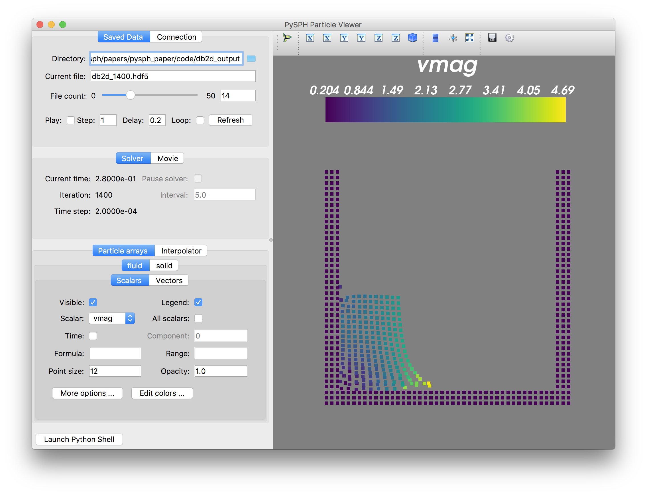
PySPH also ships with a simple 3D viewer that allows users to quickly visualize the generated output. When PySPH is installed it installs a script called pysph. The viewer is available as a sub-command of the pysph command. The viewer can be used to visualize the results of the simulation above using:

$ pysph view db2d_output

The resulting viewer after some configuration is as shown in Fig. 4. The viewer uses the Mayavi (Ramachandran and Varoquaux, 2011) Python package for 3D visualization and presents a customized UI suitable for particle visualization. One may quickly visualize a set of output files and view any number of particle arrays. The files may be viewed as a timeseries and animated. Both scalars and vectors can be viewed. In addition, the viewer may be customized with default visualization settings by overriding the Application.customize_output. This viewer is only suitable for desktops or workstations as it presents a desktop UI. It provides an interactive environment suitable for up to around 5 million particles (for a typical modern laptop or desktop).

For massive parallel simulations with many more particles one may wish to use other suitable visualization tools. The command pysph dump_vtk converts the output data files into the VTK format.

Figure 4. The built-in PySPH viewer visualizing a simple 2D dam-break problem. The color of the fluid particles indicates the velocity magnitude.

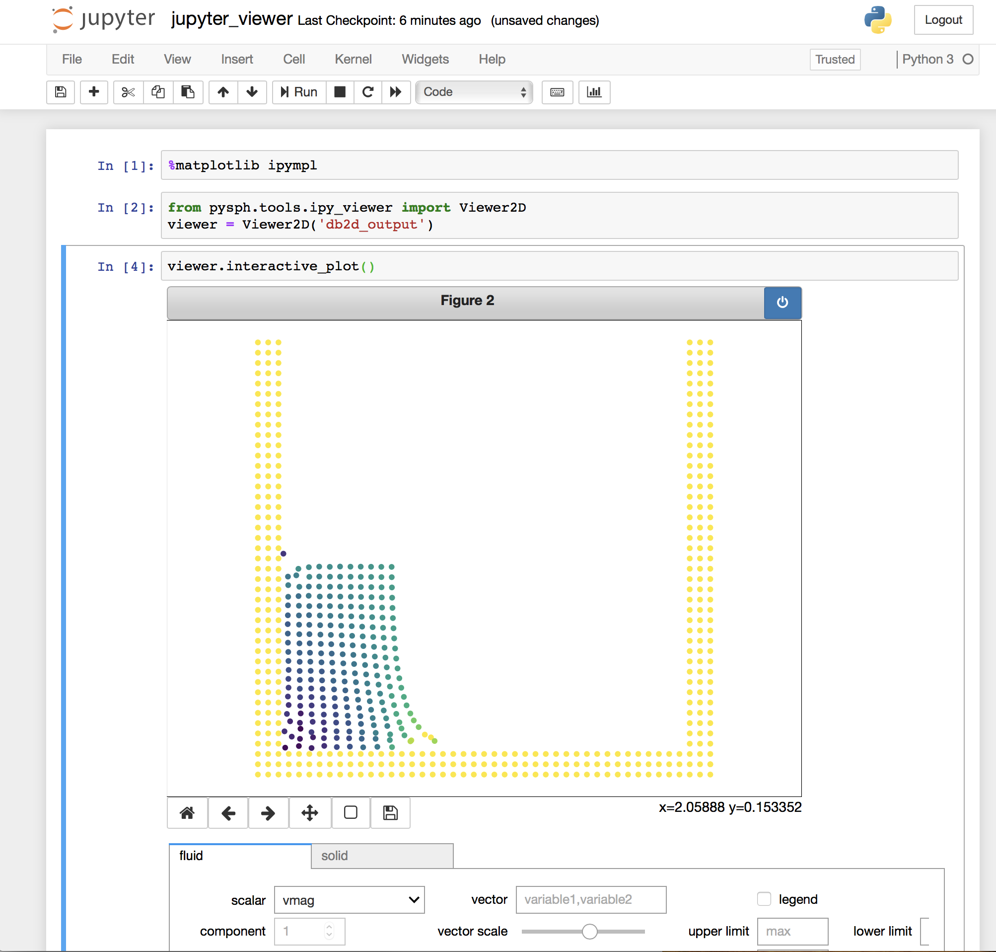
PySPH also features a viewer that allows one to share or visualize results using a Jupyter notebook (Kluyver et al., 2016). These can also be visualized on the web using a browser. This is shown in the Fig. 5. It is easy to share the results of a simulation online by hosting the files on a git repository on github.com or gitlab.com using the Binder project (Bussonnier et al., 2018). This is facilitated by the pysph binder command which when given a directory, generates suitable Jupyter notebook files as well as the other files required for the Binder project to work. One can then share this with a colleague and have a full fledged Python environment be created so anyone can view and interact with the data files. They may also perform their own analysis on the data provided in these environments.

We have created a repository with some sample results shown in this paper at https://gitlab.com/pypr/pysph_demo which contains the simulation data and can be viewed online using the binder launch link provided in the README.

Figure 5. The jupyter notebook viewer showing the 2D dam-break problem results in a browser.

For more specialized analysis, the generated output can be easily loaded into Python with a few lines of code.

⬇

from pysph.solver.utils import load

data = load(’db2d_output/db2d_4000.hdf5’)

fluid = data[’arrays’][’fluid’]

solid = data[’arrays’][’solid’]

print(fluid.x.max())

Here, the fluid and solid variables are ParticleArray instances with the saved values of the respective arrays. The last line simply prints the maximum value of the $x$-coordinate of the fluid. Any kind of post-processing and analysis may be performed using Python syntax.

In addition, PySPH provides many tools to perform a variety of post-processing using the same infrastructure that is used to run the simulations. This can be very powerful as shown in the following simple example,

⬇

from pysph.tools.interpolator import Interpolator

interp = Interpolator([fluid, solid], num_points=10000)

p = interp.interpolate(’p’)

The above example interpolates the pressure field due to the two given particle arrays, that were earlier read from the file, on a uniform mesh of 10000 points that encloses the domain. The interpolator uses the same infrastructure as the PySPH simulations and may also be passed additional parameters including a custom set of equations to change the nature of the implementation or an arbitrary distribution of points to evaluate the values on.

PySPH also provides a general purpose SPHEvaluator in the pysph.tools.sph_evaluator module. This may be passed a set of particle arrays and a collection of equations and a kernel. Internally, PySPH generates the high performance code, compiles it, and calls this code to evaluate the equations.

Thus, PySPH provides the basic building blocks to perform a variety of inter particle computations very efficiently from the convenience of high-level Python.

3.3. Underlying design

Now that the basic features of PySPH have been understood from the perspective of a user, we provide a high-level overview of how this is implemented. We explain this in the context of the Application.run() method that is called when one wishes to simulate any SPH problem (see Listing 1). The method internally performs the steps as follows:

1. Parsing of command line options passed to the script, setting up application logging, and passing the parsed command line arguments back to the user.

2. Create the solver via create_solver(), thereafter the equations using create_equations(), and then the particles by calling create_particles().

3. Optionally create any periodic or mirror boundary condition domains, and any inlets and outlets.

4. Instantiate a suitable nearest neighbor particle search (NNPS) algorithm to be used for the problem. PySPH features a variety of different NNPS algorithms as discussed in Section 2.2. These may be either set manually or be changed from the command-line.

5. The Solver.setup method is then called which passes the created particles, the equations, NNPS, and kernel to the solver. The solver is constructed with the integrator information as shown in Listing 5. This method now has all the necessary information to generate the required code for the equations and the integrator. An SPHCompiler object is delegated the task of generating the code, compiling it, and being able to call it from Python.

6. The application also sets up any user callback functions that need to be called after each step of iteration or after each stage of integration.

7. Finally, the Solver.solve method is called which performs the time integration. The integration process periodically dumps output files as configured by the user.

The generation of the high-performance code from the Python equations and integrators is an involved process. PySPH has two important classes to manage the integration of the particle properties. The Integrator steps the particle properties in time and computes the accelerations using another class called the AccelerationEval. These Python classes internally use a compiled module that implements all the high performance aspects of the computation. On the CPU, the compiled code is in the form of a Cython (Behnel et al., 2011) extension module. Whereas, on the GPU devices, these are implemented as functions provided by the underlying GPU wrapper (PyOpenCL and PyCUDA (Klöckner et al., 2012)). We discuss these in more detail in the following.

The AccelerationEval itself merely exposes a Python interface which can be called. The SPHCompiler uses an AccelerationEvalHelper class which generates the appropriate code and sets up the underlying high-performance module. A similar strategy is employed for the Integrator.

All the acceleration equations follow a very similar structure where the methods of a group of equations are invoked for each particle. Taking advantage of the similarity, we employ a technique commonly used in web development called templating to write the common code once and dynamically substitute the variable parts. PySPH uses the mako (Bayer et al., 06 ) template library for this and auto-generates the Cython code using a mako template.

To understand this better we consider the case of dam-break problem. We have two groups involving two different particle arrays and five different equations. We can break this up into pair-wise interactions between the respective particle arrays as below:

1. For all the fluid particles, evaluate the EOS.

2. For all the solid particles, evaluate the EOS.

3. For all the fluid particles (as destination), evaluate the ContinuityEquation and MomentumEquation due to the fluid particles.

4. For all the fluid particles (as destination), evaluate the ContinuityEquation and MomentumEquation due to the solid particles.

5. For all the solid particles (as destination), evaluate the ContinuityEquation due to the fluid particles.

Consider the continuity equation evaluated on the fluid by the fluid itself. The pseudo-code (written with a Python syntax) to evaluate this would be as shown in Listing 7. As can be seen in the listing, we first set the initial value of the property by calling the method implemented by the user and then call the loop with the appropriate neighbors. Clearly, executing this in parallel would require a lot more work and computation of the neighbors is itself fairly involved. However, the basic steps of the SPH computation are essentially what is shown in the algorithm. We write a mako function that generates the code necessary for each pair of particle arrays given a group of equations. Depending on the combination of particle arrays and equations, this is automatically expanded out into many lines of code. This is a very powerful approach because the template is written only once.

Listing 7: Pseudo-code for the evaluation of a single equation.

⬇

for d_idx in range(n_dest_particles):

continuity_fluid.initialize(d_idx, fluid.arho)

for d_idx in range(n_dest_particles):

for s_idx in fluid.neighbors(d_idx):

DWIJ = kernel.gradient(...)

VIJ = [fluid.u[d_idx] - fluid.u[s_idx], ...]

continuity_fluid.loop(

d_idx, s_idx, fluid.arho, fluid.m, DWIJ,

VIJ

)

The key part of generating the high performance implementation of the equations is delegated to the compyle package (Bhosale and Ramachandran, 2020; Ramachandran et al., 18 ). Since Cython is very similar to Python, we create equivalent Cython classes and determine the types of the variables passed to the equations using the type information from the particle arrays. The integrator is also similar and another mako template is used for this. All of the generated code (which includes the high-performance classes for equations and integrator steppers) is injected into a Cython file, automatically compiled and linked, and called transparently by PySPH.

Adding support for execution via OpenMP requires rewriting the generated acceleration evaluation to include OpenMP loops, managing issues like false sharing carefully, and dealing with the special variables like VIJ, DWIJ etc. However, all of this needs to be done just once and when implemented, the code can be executed on multiple cores. It is important to note that the user-facing code does not change.

On a GPU, this process is similar but requires a lot more effort. The first issue is that on OpenCL or CUDA we are not able to create classes that are analogous to the Cython ones. Instead we create GPU kernels for each function and invoke them. The user code in the equations and integrator steps also must be transpiled into OpenCL or CUDA. This is done by a special transpiler which takes low-level Python code and converts it to efficient C code. The transpiler is part of the compyle package. This allows PySPH to generate high-performance GPU code on the fly. The rest of the process is similar and uses mako templates to generate GPU code.

It is important to note that there are only 4 mako templates used in PySPH. There are two for the CPU code generation (one for the integrator and one for the acceleration evaluation) and two more for the GPU. Thus, by employing mako templates in this fashion we are able to significantly reduce the complexity of our implementation without losing a significant amount of readability.

As discussed earlier, there are some severe restrictions in what code can be written in the various equation methods. The Python programming language uses a global interpreter lock (GIL) in order to ensure thread safety. Hence, any computations involving multiple threads requires that no Python objects be manipulated. The PySPH particle arrays expose low-level memory views of the underlying properties and constants. The equations are therefore written to only manipulate these properties and constants. This can be done entirely in parallel and is one of the most time-consuming parts of an SPH simulation. Thus, we do not encourage users to write any arbitrary Python code in the equation methods. The compyle package also follows the same philosophy and users write a restricted subset of Python where only manipulation of one dimensional, contiguous numpy arrays are allowed. Memory allocation is not allowed and Python objects may not be created. More details on the restrictions are provided in (Bhosale and Ramachandran, 2020). Compyle provides important parallel algorithms like the elementwise operations, reductions, and scans. PySPH uses compyle for code generation, transpilation, and some of the parallel algorithms.

Thus far the general features and functioning of the high-level framework have been discussed. It is important to note that it is possible to use PySPH as a library too. Much of the functionality is usable outside of the context of the framework. For illustrative purposes, let us consider evaluating the continuity and momentum equations mentioned earlier on a particle array this can be done using the code shown in listing 8. Here, the SPHEvaluator can be used to evaluate the effect of the equations on the particles. This allow a user to reuse the infrastructure to perform a variety of computations with particles and their nearest neighbors.

Listing 8: Code to evaluate a collection of equations.

⬇

from pysph.base.utils import get_particle_array

from pysph.base.kernels import QuinticSpline

from pysph.tools.sph_evaluator import SPHEvaluator

pa = get_particle_array(name=’fluid’, x=x_data, y=y_data, ...)

eqs = [Group(equations=[

ContinuityEquation(dest=’fluid’, sources=[’fluid’]),

MomentumEquation(dest=’fluid’, sources=[’fluid’])]

)]

evaluator = SPHEvaluator(

arrays=[pa], equations=eqs, dim=2, kernel=QuinticSpline(dim=2)

)

evaluator.evaluate()

To summarize the overall design, PySPH uses a high-level Application class to abstract out the basic pieces involved in an SPH computation. Python is used to create the particles using numpy arrays, specify the particle interactions, and integration process. This information is then extracted in a systematic way and high-performance code is generated as necessary to compute the particle interactions on different HPC hardware.

3.4. Advanced features

PySPH also supports some advanced features that are useful in certain contexts. In this section we discuss two such features, iteration of a group of equations while evaluating the RHS and inlet and outlet boundary conditions. These features are used in some of the results presented.

3.4.1. Iterated groups

In SPH, some schemes like ISPH, pressure is determined using pressure Poisson equation (PPE), which is solved iteratively. In order to evaluate a group of equations ‘iteratively‘ in between other groups which are being solved once per time step, we have implemented iterated Groups in PySPH.

Iterated Groups are Groups as explained in Section 3.2 with an additional feature to iterate within a time step. In Listing 9, we show the set of equations which are to be iterated in order to get a converged solution. The equations PressureCoeffmatrixiterative and PPESolve (dest and sources are not shown) are grouped together and put in an iteration group as indicated by the iterate keyword. One may also specify the minimum and maximum number of iterations required. The equation PPESolve overloads a method called converged. This converged function returns $-1$ when the iterations have not converged and $+1$ otherwise. The entire group of equations is re-executed until all equations have converged or if the maximum number of iterations is reached. The convergence criterion is dependent on the algorithm chosen. For example, if one wishes to ensure that the average change to the pressure in the entire simulation is less than a prescribed tolerance, then one can continue iteration until this criterion is attained by returning a suitable value.

Listing 9: Code showing the usage and implementation of iterated Group in PySPH.

⬇

Group(equations=[

Group(equations=[

PressureCoeffMatrixIterative(...),

PPESolve(...)

])

], iterate=True, min_iterations=2,

max_iterations=1000)

In (Muta et al., 2019) we implement a simple iterated scheme for incompressible SPH where a system of equations is solved using Jacobi iterations. This is done using an iterated group.

3.4.2. Inlet/outlet boundary conditions

The imposition of inlet/outlet boundary condition is non-trivial in SPH. The method to implement differs from scheme to scheme. In (Negi et al., 2020), we explored various type of inlet/outlet boundaries. An inlet/outlet boundary generally requires ghost particles to obtain the properties from the fluid. PySPH provides the equations which are to be used for interpolation, the stepper to move the particles as explained in Section. 3.2, and a callback function to convert the inlet/outlet particles to fluids or vice-versa.

In PySPH, the class InletOutletManager (IOM) manages all the work needed for a inlet/outlet boundary. In order to create an InletOutletManager object, we need information of all inlets and outlets in the form of start/end coordinates, outward normal, additional equations etc. The IOM performs the following tasks:

1. Create a callback which adds or deletes the particles for fluid to inlet/outlet.

2. Create ghost particles.

3. Pass stepper functions to the solver.

4. Provide interpolation equations to the scheme.

Currently, PySPH implements all the inlets/outlets described in Negi et al. (2020).

3.5. Distributed execution

As discussed earlier, one may use MPI to run PySPH applications in a distributed mode. This works by making use of another sister package called PyZoltan (Puri et al., 13 ), which is a wrapper to the ZOLTAN package (Boman et al., 1999, 2012). PySPH uses PyZoltan to partition the particles across multiple computers. A ghost region is defined over each processor and any particle in these regions are shared between appropriate processors. PySPH implements the necessary parts that allow ZOLTAN to distribute and gather the particles. This is all managed by a ParallelManager available in the pysph.parallel package. The parallel manager is invoked each time the particles have moved and the properties are changed. Updated properties of particles in the ghost region are exchanged with other processors as required. Any particles that have moved outside the region of a given process are shifted to the appropriate processor. PyZoltan also manages the load balancing so the particles are evenly distributed. More details are available in Puri et al. (2013).

3.6. Reproducibility

PySPH aims to be a research tool that facilitates reproducible computational science. The first important feature in this context is that PySPH examples ship with the software and are designed to be reusable. When PySPH is installed, an executable pysph is made available and this can be used to execute any of the shipped examples. There are around 90 examples at various levels of maturity. Many of the standard benchmark problems seen in the literature are available and these also include post-processing of the results along with comparisons with exact or experimental results in some cases. For example, if we execute

$ pysph run taylor_green --help

We will see that we can execute this standard problem with 7 different SPH schemes that are already implemented in PySPH. The scheme can be chosen by using the --scheme scheme-name command line argument. When the problem finishes executing, the results are also compared with the exact solution. Many of these examples support command line arguments that make it possible to perform parametric studies.

Furthermore, as the examples are part of PySPH, a user may easily subclass the example to modify it with a minimum of code replication by importing the example class as from pysph.examples.taylor_green import TaylorGreen.

In addition to this, PySPH integrates with a sister package called automan (Ramachandran, 2018). The present work and our recent papers in the area of SPH are reproducible (Ramachandran and Puri, 2019; Muta et al., 2019; Negi et al., 2020; Ramachandran et al., 2019). What we mean by this is that every figure produced in these papers is fully automated. We provide a link to the repository so anyone may reproduce all the computations (or a part of them) by running a single command. The advantages of this to the readers and researchers are clear. We have also found that investing time in automation is also very valuable to the authors. This is discussed in detail in (Ramachandran, 2018).

Thus, PySPH is a powerful framework for reproducible research in particle methods in general and SPH in particular. Many of the tools created for PySPH may be used in other contexts.

3.7. Software engineering

PySPH follows some important and useful software engineering practices to improve the quality of the code.

• Open code and repository: Our code is open source and ships with a liberal BSD 3-clause license. While the code is copyrighted, it may be reused by anyone for any purpose and may also be redistributed. The code is openly available on https://github.com/pypr/pysph and does not require any formal process to access or download. git is used for version control.

• Testing: We have implemented a large number of unit tests and functional tests that ensure correctness of our code to the extent possible. The test coverage can be further improved, however, we already have close to 900 tests. These tests are executed on Linux and Windows computers. Links to the test results are available on the project page. The tests include checking that the kernels are accurate and satisfy the various integral properties, correctness of the nearest neighbor computations for the different methods and for the CPU and GPU backends, correctness of the various methods of the particle array. The parallel execution with OpenMP and MPI is tested as compared to a serial execution for some time steps for a few problems in two and three dimensions. The acceleration evaluation is tested for simple equations that exercise all of the various features on all the supported backends, the integrators are also tested on simple problems. All of the examples that are included are compiled and executed for a single time step. We do not test the specific schemes as that would be very time consuming. The current set of tests take about half an hour to execute on Travis-CI and about 15 to 20 minutes on appveyor. When a bug is found a suitable test case is introduced.

• Continuous Integration(CI): PySPH employs continuous integration testing. New features and bug fixes are added in the form of pull-requests. When these pull-requests are submitted, all the tests are executed on Linux and Windows machines automatically. This immediately ensures that any existing functionality is not broken by the new feature. This is standard practice for most popular open source software.

• Online documentation: The PySPH documentation, which is extensive, is automatically built every time the master branch of the code repository is changed. The documentation is hosted at https://pysph.readthedocs.io and is available for anyone to read.

• Support: Bug reports and issues may be filed on the github web interface by any user. These are attended to by the PySPH developers as time permits. A mailing list is also available at https://groups.google.com/d/forum/pysph-users where users may ask questions and also see any PySPH related announcements.

We believe that by using well established software engineering practices, PySPH will be easy to use, well supported, and retain good quality over time.

4. Sample results

In this section, we demonstrate the capabilities of PySPH by solving a wide variety of problems in different fields, including incompressible and compressible fluid dynamics, and elastic dynamics. At the end of this section we provide qualitative indicators analysing the performance of PySPH on CPU (both single and multi-cores) and GPU architectures. The results presented here are only indicative of the breadth of problems that can be handled. We do not provide all the details of the parameters used in the simulations. However, the source code for the simulations presented are available at the repository https://gitlab.com/pypr/pysph_paper.

4.1. Taylor-Green Vortex

Taylor-Green vortex is a standard test case for incompressible flows. This problem is periodic in both $x$ and $y$ directions and has no boundaries. This problem admits an exact solution given by,

$$\begin{split}u&=-Ue^{bt}\cos(2\pi x)\sin(2\pi y),\\ v&=Ue^{bt}\sin(2\pi x)\cos(2\pi y),\\ p&=-U^{2}e^{2bt}(\cos(4\pi x)+\cos(4\pi y))/4,\\ \end{split}$$

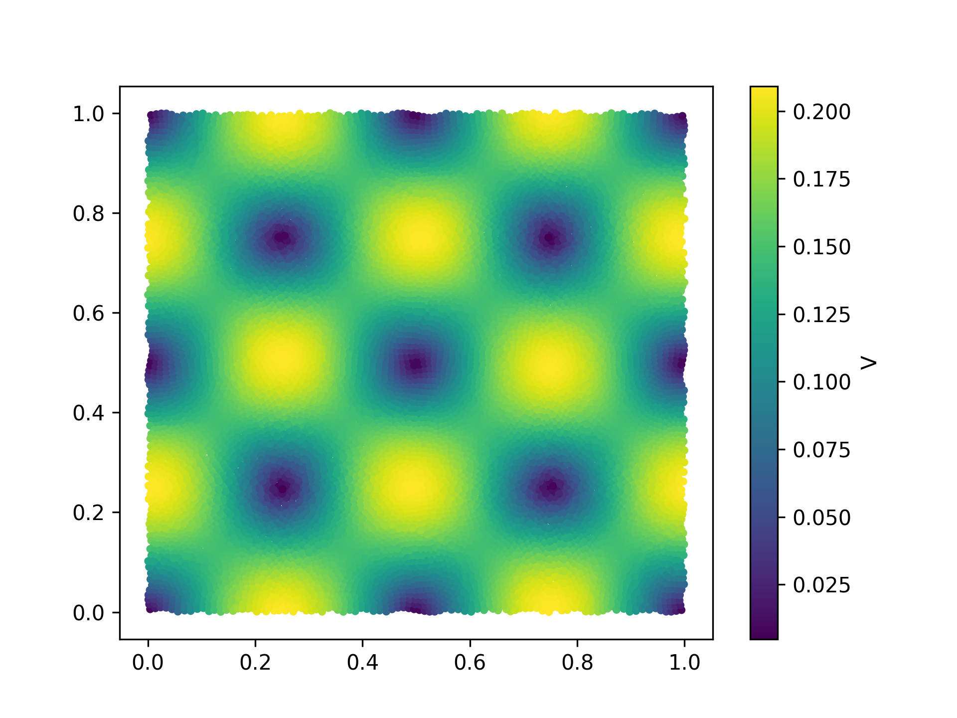
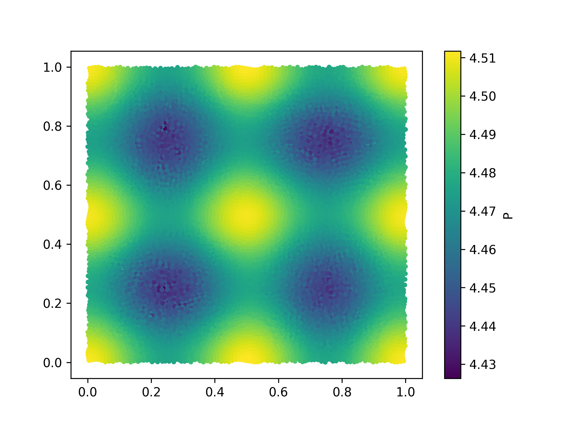
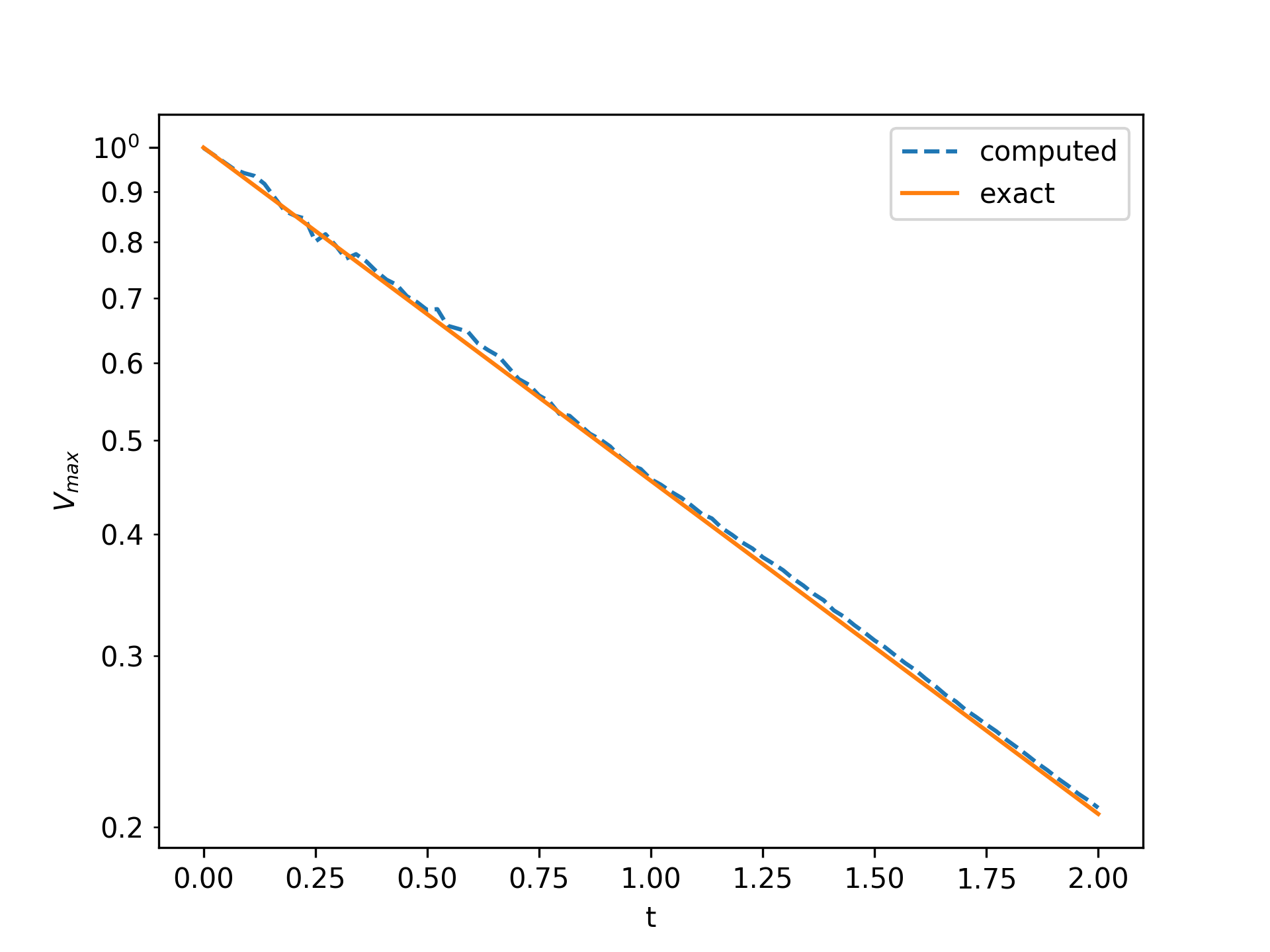
where $U$ is the maximum velocity, $b=-8\pi^{2}/Re$, and $Re$ is the Reynolds number. In order to simulate this problem, we consider a periodic domain of size $1m\times 1m$ and use the Entropically Damped Artificial Compressible SPH (EDAC-SPH) scheme (Ramachandran and Puri, 2019). The maximum velocity, $U$ and Reynolds number, $Re$ are set to $1$m/s and $100$ respectively. The domain is discretized by $100\times 100$ particles, and $h/\Delta x=1.2$, where $\Delta x$ is the particle spacing. In Fig. 6, we plot the velocity and pressure at $t=2$ seconds. The initial pattern is maintained, with the decay in velocities as expected. In Fig. 7, we plot the maximum velocity compared with the expected theoretical result and the results are in agreement.

Figure 6. Velocity magnitude, and pressure distribution for Taylor-Green vortex at $t=2$s using EDAC (Ramachandran and Puri, 2019).

Figure 7. Maximum velocity decay in Taylor-Green vortex compared with the exact solution.

4.2. Lid-driven cavity

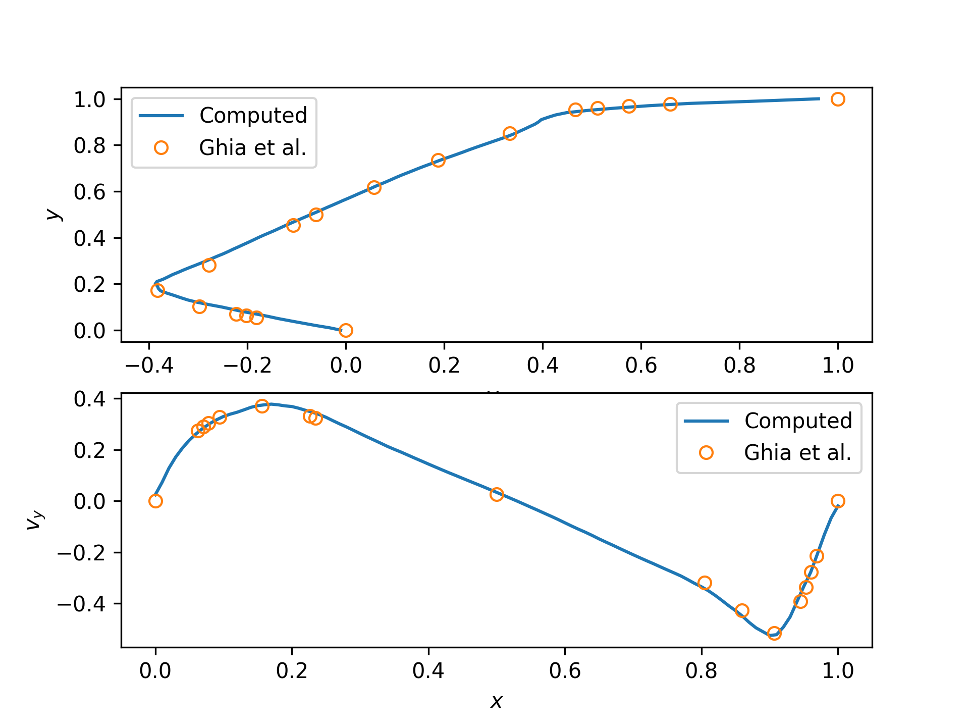
The lid-driven cavity is a classic benchmark problem. We consider a 2D cavity of size $1m\times 1m$ with the top boundary moving with a velocity $U=1$m/s and use the Transport Velocity Formulation (TVF) (Adami et al., 2013) scheme. The Reynolds number, $Re=1000$ is considered. $50\times 50$ particles are used to discretize the problem and $h/\Delta x=1.0$. The quintic spline kernel is used. In Fig. 8, we compare the velocity profile at the centerline with Ghia et al. (1982). The results are in agreement showing the validity of the TVF scheme for this problem.

Figure 8. Velocity profiles $u$ vs. $y$ and $v$ vs. $x$ for the lid-driven-cavity problem at Re = 1000. Particle discretization of $100\times 100$. We compare the results with those of Ghia et al. (1982).

4.3. Flow past a bluff body

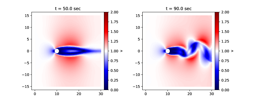
Here we simulate the flow past a circular cylinder in an internal flow. This test case is used to demonstrate the implementation of inlet outlet boundary conditions in SPH. The inlet velocity is set to $1$m/s, the diameter of the cylinder is $2$m, and the Reynolds number is 200. The domain is discretized such that there are $20$ particles along the diameter of the cylinder. The inlet continuously feeds the particles into the fluid domain with desired initial properties, while the outlet removes the fluid particles smoothly from the flow. Further details of the theory and implementation can be found at (Negi et al., 2020).

Fig. 9 shows the velocity magnitude of the flow past the cylinder. The vortex shedding at time $t=90$s is seen clearly. As a quantitative validation we determine the lift and drag coefficients for the cylinder, which have been found to be $1.524$ and $0.722$. There is a 5% difference from those reported by (Tafuni et al., 2018). The Strouhal frequency is found as 0.2 and this differs from other reported results by 2%.

Figure 9. The plots showing the velocity magnitude of the flow past a circular cylinder at $t=50.0$s and at $t=90.0$s.

4.4. Dam break in 3D

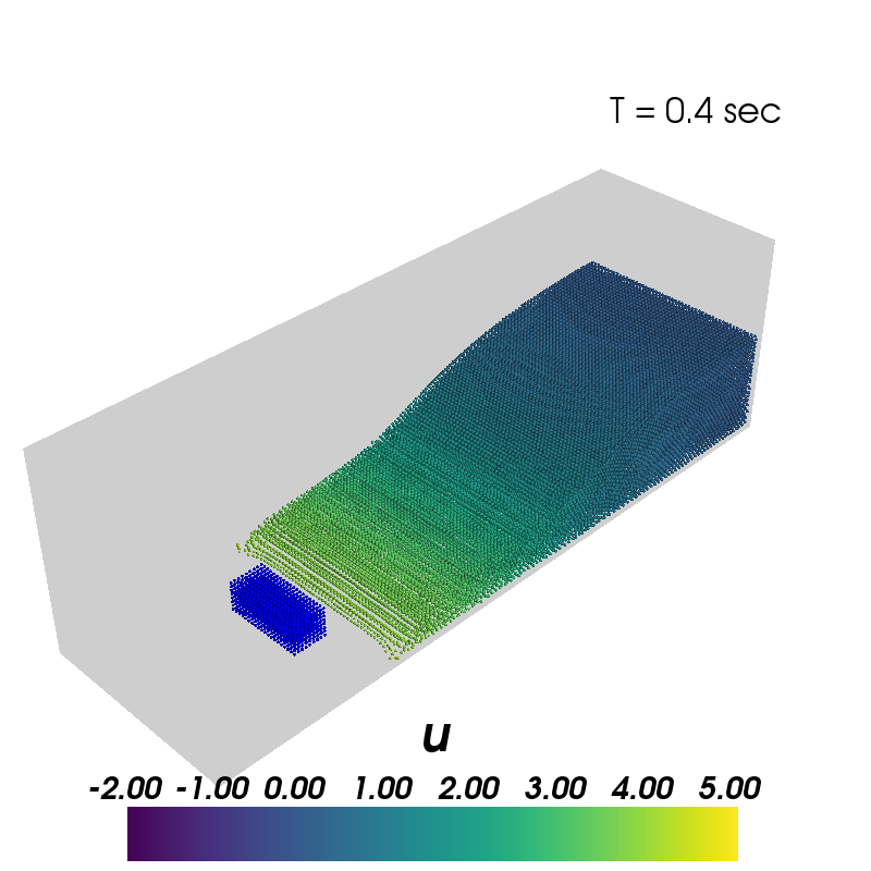
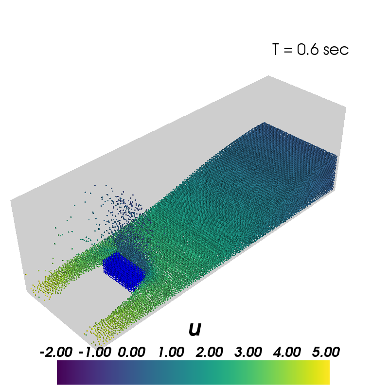
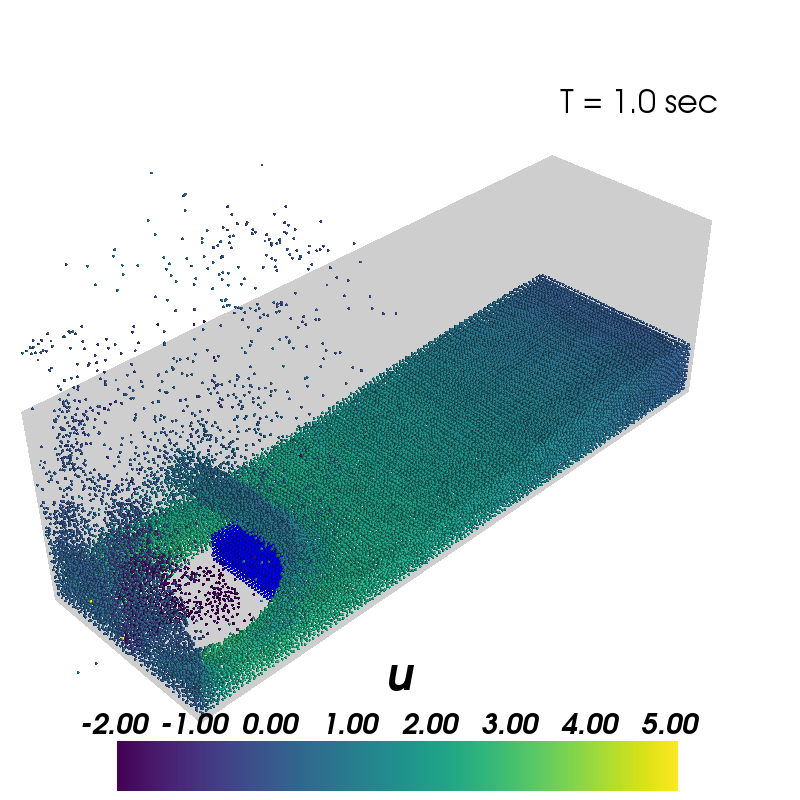
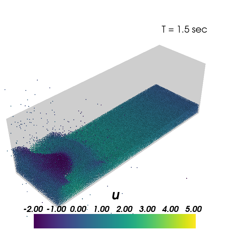
A three-dimensional dam break is simulated using a simple iterative ISPH (SISPH) scheme which is discussed in greater detail in Muta et al. (2019). This is an iterative incompressible scheme which uses the iterated Group feature as discussed in Section 3.4.1. A fluid column is released from one side of a tank under the influence of gravity, an obstacle is placed in the path of the fluid flow. In Fig. 10, we show the $x$-component of the velocity at different time steps. As can be seen, the flow splashes at the obstacle.

Figure 10. Figure showing the velocity magnitude of the particles in the three dimensional dam break simulation at various time instances.

4.5. Kelvin-Helmholtz instability

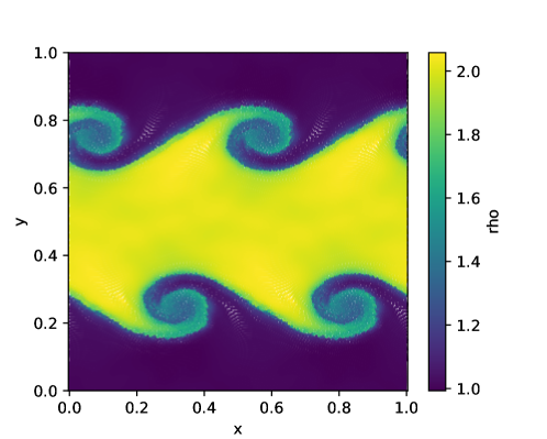
This example demonstrates the modeling of fluid instabilities and compressible flows in PySPH. We model Kelvin-Helmholtz instability, which exhibits the subsonic instabilities of a compressible gas. Kelvin-Helmholtz instability manifests at the interface of two fluids moving with two different velocity profiles. The problem is periodic in both $x$ and $y$ directions. A sinusoidal velocity perturbation is given in the $y$-direction as given in Robertson et al. (2010). This is simulated using the conservative reproducing kernel SPH (CRKSPH) (Frontiere et al., 2017) that is available in PySPH. The density profile of the particles is shown in Fig. 11. We expect to see the roll-up of the shear layer, which is captured well by the scheme.

Figure 11. Kelvin-Helmholtz instability simulation using CRKSPH (Frontiere et al., 2017) with $200\times 200$ particles. Shown is the density $\rho$ of the particles at $t=2$s.

4.6. Sod’s shock tube

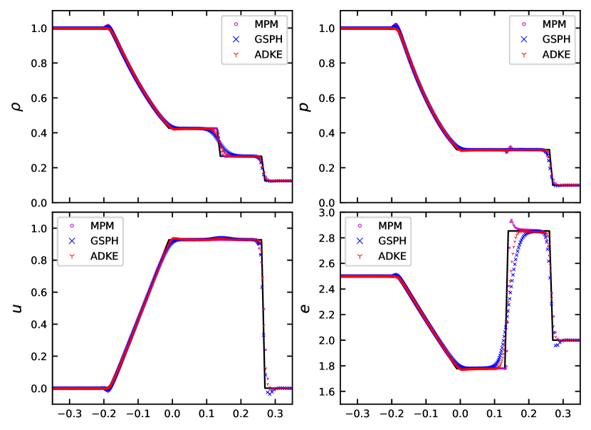
Sod’s shock tube problem, considered a classic 1D problem in compressible fluid dynamics. PySPH has several different compressible SPH schemes to solve such problems. Here we simulate the problem using three schemes: Adaptive Density Kernel Estimation technique (ADKE) (Sigalotti et al., 2006), Monaghan-Price-Morris (MPM) scheme (Price, 2012), Gudunov type Smoothed Particle Hydrodynamics (GSPH) (Puri and Ramachandran, 2014). For the simulation we use $720$ particles of which $640$ are placed with uniform spacing in the domain $x\in[-0.5,0)$ and $80$ are placed with uniform spacing in the domain $x\in[0,0.5]$. $(\rho_{l},p_{l},v_{l})=(1.0,1.0,0.0)$ and $(\rho_{r},p_{r},u_{r})=(0.125,0.1,0)$ on the left and right sides of the diaphragm which is placed at $x=0$. The results of the simulation are compared with the exact solution in Fig. 12. For a detailed discussion of this problem, see (Puri and Ramachandran, 2014).

Figure 12. 1D Sod’s shock tube at $t=0.1$. Three schemes, ADKE, MPM and GSPH are used for the simulation. Comparison of the exact solution vs profiles of density, pressure, velocity, and energy of all the particles is shown.

4.7. Elastic deformation of colliding rings

In this example we simulate collision of two rubber rings. This example is used to demonstrate the ability of PySPH in modelling elastic dynamics. We have implemented the formulation proposed by Gray et al. (2001) to model the elastic dynamics. Two rings are initialized with a velocity such that they are moving towards each other. Figure 13 shows the velocity magnitude at two different times. At $t=20\mu$s the rings have collided with each other and start to deform. At $50\mu$s, more significant deformation is seen, eventually the two rings reverse their velocities although this is not shown in the figure.

Figure 13. Velocity magnitude plots of the collision of elastic rings at times $t=20\mu$s and $t=50\mu$s.

4.8. Sand in a rotating drum

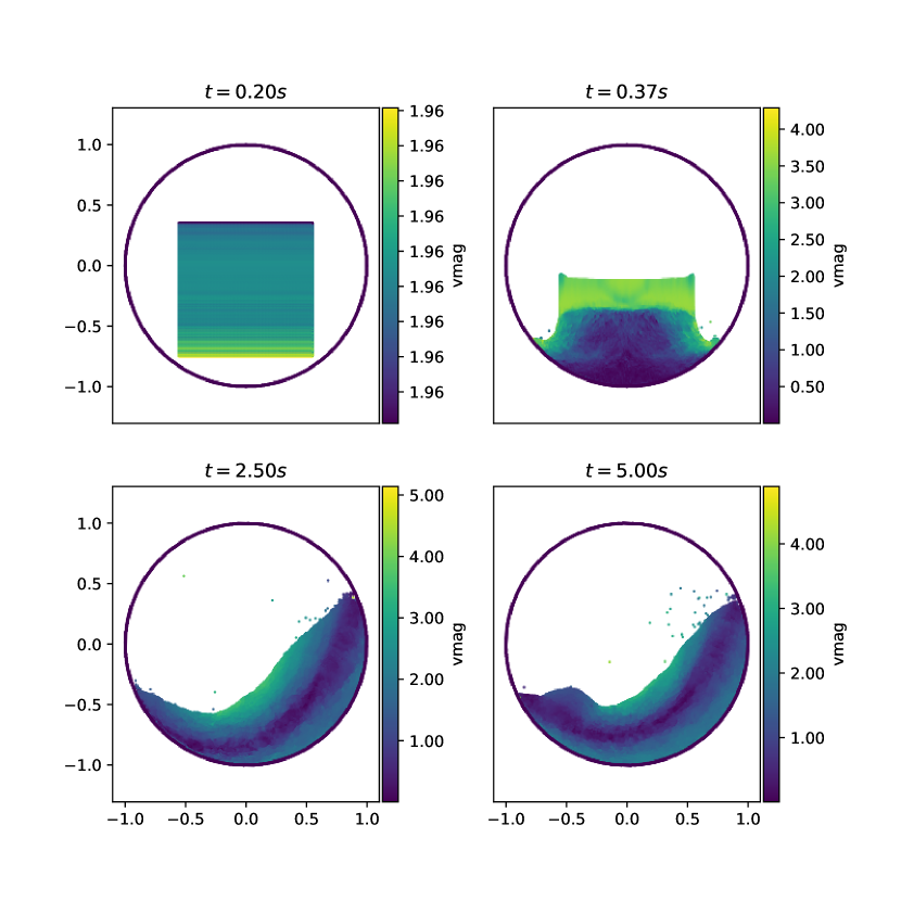
This example demonstrates an implementation of the Discrete Element Method (DEM) implemented using PySPH. The motion of sand in a rotating drum is simulated. The dynamics of the particles follow the formulation by Cundall and Strack (Cundall and Strack, 1979) and Luding (Luding, 2008). The drum is initially static and starts rotating with an angular velocity of 5 rad/s after the sand settles down. Fig. 14 shows the arrangement of the sand particles, the top row depicts the results when the drum is not rotating, while the bottom row is when the drum is rotating. This shows that PySPH provides the features required to implement a variety of different meshless methods.

Figure 14. Positions of the sand in a drum, color indicates the velocity magnitude. The top row depicts the results when the drum is not rotating, and the bottom row is when the drum is rotating.

4.9. Performance analysis

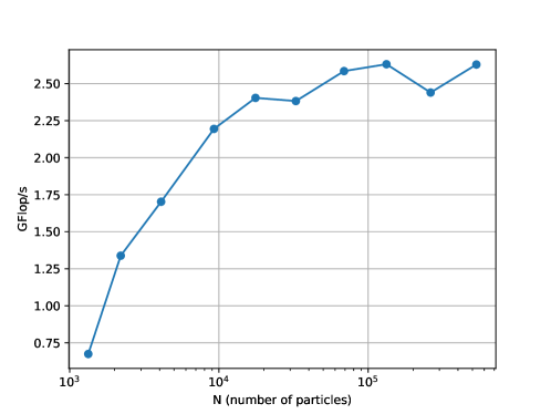
In this section we discuss the performance of PySPH. Fig. 15 shows the number of floating point operations per second (FLOPS) for a simple simulation of a cube-shaped block of water falling in free-space under the influence of gravity run on an i3-6100 CPU (single-core) while varying the number of particles. We note that we compute the fluid dynamic equations on the water particles during this computation. We use the Performance Application Programming Interface (PAPI) (Terpstra et al., 2010) to count the FLOPS using the CPU hardware counters.

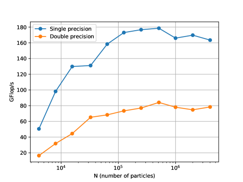
We see that on the CPU, the performance peaks at about $2.6$ GFlop/s. Our performance compares favorably with the singular value decomposition of an $800\times 800$ matrix using numpy.linalg.svd which uses the Intel MKL (Wang et al., 2014) implementation and is at $2.49$ GFlop/s that reduces as the matrix size increases. It is also comparable to a 1D discrete Fourier transform using numpy.fft.fft which also uses the MKL implementation and shows a peak performance of $4.18$ GFlop/s. On the GPU, counting the number of FLOPS accurately is more difficult. We measure the performance of the loop kernel that evaluates the equations for each pair of source and destination particles, which in the current example is the most expensive kernel call and takes 60% of the total execution time. Fig. 16 shows the FLOPS for the loop kernel on a Tesla T4 GPU using single and double precision. This performance peaks at about 180 GFlop/s using single precision, and about $80$ GFlop/s using double precision. We note that at this point our GPU code still requires optimizations and that the performance will be improved in the future.

Figure 15. FLOPS vs. number of particles for a cube shaped block of water in free-fall on an i3-6100 CPU.

Figure 16. FLOPS vs. number of particles for the loop kernel of a cube shaped block of water in free-fall using single and double precision on a Tesla T4 GPU.

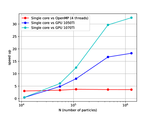
We show the performance and scale-up of PySPH on multi-core CPUs, and GPUs by comparing the time taken to simulate the dam break 3D problem discussed earlier in this section with varying number of particles on different platforms. We obtain the scale-up seen with respect to the time taken on a single-core CPU. We use an Intel i5-7400 CPU with 4 physical cores, an NVIDIA 1050Ti GPU, and an NVIDIA 1070Ti GPU. The speed-up obtained is shown in the Fig. 17. It can be seen that on a CPU with OpenMP there is nearly a 4 fold speed up. On the GPU with the same source code we obtain speed-up of around 17 and 32. It is to be noted that the GPU simulations are made with single precision.

Figure 17. The comparison of number of particles vs. speed-up on different platforms with respect to the time taken by single core CPU for the three dimensional dam break.

The multi-core CPU support in PySPH is more mature than the GPU support. To demonstrate its efficiency, we consider a 3D dam-break problem with $0.17$M and $1.4$M particles and measure the speed-up obtained when using OpenMP. Fig. 18 shows the results as the number of threads are increased on a machine with dual-Intel Xeon E5-2650 v3 CPUs resulting in a total of 20 physical cores. We obtain a speed-up of around $18$ with the 20 cores for both the problem sizes. This shows that the OpenMP implementation scales well.

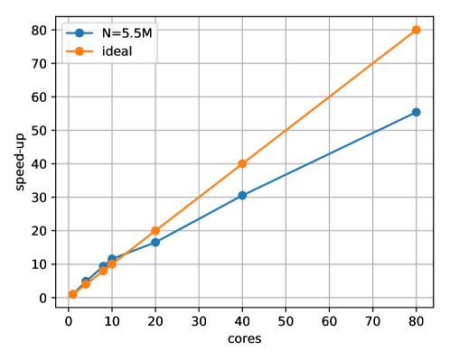
We show the speed-up with MPI for the same problem in the Fig. 19 with $5.5$M particles. We obtain a speed-up of $55$ with 80 MPI processes on a Cray cluster (with Cray OS, 2X Intel Skylake 6148 2.4 GHz 20C processors and Cray Aries with Dragonfly topology interconnect network) with respect to a single-core simulation. This shows that PySPH performance scales reasonably well when run in a distributed mode. We would like to add that this aspect of PySPH can be further optimized and this is something that will be done in the future.

	PySPH v1.0b1	DualSPHysics v5.0
1-core (in secs)	329.55	146.63
OpenMP 4-cores (in secs)	90.82	41.26

Table 2. Comparison of PySPH with DualSPHyics (Crespo et al., 2015) on single-core CPU, and with OpenMP on 4-cores.

In order to see how well PySPH performs with a well-established, fast implementation, we compare the performance of the CPU execution with that of DualSPHysics v5.0 (Crespo et al., 2015) on a Intel i5-7400 single and multi-core setup. In Table 2 we note that our performance is around twice as slow. This is because DualSPHysics uses a customized loop to compute the neighbors and the particle accelerations in one step. Although this is fast, it does not allow us to replace the NNPS algorithm easily or perform iterated evaluations of equations efficiently. We are contemplating using this approach in the future for the weakly-compressible schemes in PySPH. Our design allows us to implement this transparently.

In this section, we have demonstrated that the automatic code generation produces code that is easy to write but still retains good performance with good scaling on OpenMP and MPI. The code can be executed on a GPU, however, the performance still requires further optimization.

Figure 18. The OpenMP speed-up with respect to single core CPU with 0.17M and 1.4M particles in a 3D dam-break problem.

Figure 19. The MPI speed-up with respect to single core CPU with 5.5M particles in a 3D dam-break problem.

5. Conclusions and future directions

This article provides an overview of the design of PySPH, a powerful and general purpose framework for smoothed particle hydrodynamics simulations. We demonstrate how a standard problem can be solved using the framework using a minimum of code. The overall design and underlying details of how this is accomplished is shown. Various results demonstrating the wide applicability of PySPH are shown.

PySPH is a unique framework for the following reasons:

• One can implement an entire SPH formulation in pure Python with very little code. This includes, SPH kernels, inter-particle interactions, and integrators.

• This pure Python code can be executed without any changes on multi-core CPUs, GPUs, and on a cluster using MPI.

• It implements many of the current state-of-the-art SPH schemes with over twenty schemes supporting different problems including weakly-compressible, incompressible, compressible fluid flow, elastic dynamics, DEM, etc.

• It provides over ninety examples that can easily reused by researchers.

• It provides many useful utilities including a built-in 3D viewer, the ability to share results through jupyter notebooks, and Binder.

• Makes it easy to perform reproducible research in the area of particle methods.

These show that PySPH is a powerful tool that can be useful for research in particle methods. PySPH uses object-orientation to provide powerful interfaces that facilitate significant code reuse. Code generation is used heavily in PySPH so as to generate hardware specific implementations on both multi-core CPUs as well as GPUs from the same initial Python code. Finally, the use of standard software engineering practices improve quality, and accessibility to the software and documentation.

We plan the following improvements:

• Improved support for adaptive particle resolution.

• Improved performance on GPUs and support for multiple GPUs.

• Improved parallel performance with MPI.

• Implementation of tree-codes to facilitate gravitational interactions, long-range electromagnetic forces, and the like.

• Implementation of other meshless methods like the RKPM and MLS methods.

PySPH is already being used by some researchers across the world and we believe that its usage will increase given its many features.

References

- Lucy (1977) Lucy, L.B.. A numerical approach to testing the fission hypothesis. The Astronomical Journal 1977;82(12):1013–1024.
- Gingold and Monaghan (1977) Gingold, R.A., Monaghan, J.J.. Smoothed particle hydrodynamics: Theory and application to non-spherical stars. Monthly Notices of the Royal Astronomical Society 1977;181:375–389.
- Crespo et al. (2015) Crespo, A.J., Domínguez, J.M., Rogers, B.D., Gómez-Gesteira, M., Longshaw, S., Canelas, R., Vacondio, R., Barreiro, A., García-Feal, O.. Dualsphysics: Open-source parallel cfd solver based on smoothed particle hydrodynamics (sph). Computer Physics Communications 2015;187:204–216.
- Springel et al. (2020) Springel, V., Pakmor, R., Zier, O., Reinecke, M.. Simulating cosmic structure formation with the gadget-4 code. arXiv preprint arXiv:201003567 2020;.
- Cercos-Pita (2015) Cercos-Pita, J.L.. Aquagpusph, a new free 3d sph solver accelerated with opencl. Computer Physics Communications 2015;192:295–312.
- Price et al. (2018) Price, D.J., Wurster, J., Tricco, T.S., Nixon, C., Toupin, S., Pettitt, A., Chan, C., Mentiplay, D., Laibe, G., Glover, S., et al., . PHANTOM: A smoothed particle hydrodynamics and magnetohydrodynamics code for astrophysics. Publications of the Astronomical Society of Australia 2018;35:e031. doi:10.1017/pasa.2018.25.
- Koschier et al. (2019) Koschier, D., Bender, J., Solenthaler, B., Teschner, M.. Smoothed Particle Hydrodynamics Techniques for the Physics Based Simulation of Fluids and Solids. In: Jakob, W., Puppo, E., eds. Eurographics 2019 - Tutorials. The Eurographics Association; 2019:URL: https://diglib.eg.org:443/xmlui/handle/10.2312/egt20191035. doi:10.2312/egt.20191035.
- Shadloo et al. (2016) Shadloo, M.S., Oger, G., Touze, D.L.. Smoothed particle hydrodynamics method for fluid flows, toward industrial applications: Motivations, current state, and challenges. Computers & Fluids 2016;136:11–34.
- Hopkins (2015) Hopkins, P.F.. A new class of accurate, mesh-free hydrodynamic simulation methods. Monthly Notices of the Royal Astronomical Society 2015;450(1):53–110. doi:10.1093/mnras/stv195.
- Bilotta et al. (2016) Bilotta, G., Hérault, A., Cappello, A., Ganci, G., Del Negro, C.. Gpusph: a smoothed particle hydrodynamics model for the thermal and rheological evolution of lava flows. Geological Society, London, Special Publications 2016;426(1):387–408. doi:10.1144/SP426.24.
- Amicarelli et al. (2020) Amicarelli, A., Manenti, S., Albano, R., Agate, G., Paggi, M., Longoni, L., Mirauda, D., Ziane, L., Viccione, G., Todeschini, S., et al. Sphera v. 9.0. 0: A computational fluid dynamics research code, based on the smoothed particle hydrodynamics mesh-less method. Computer Physics Communications 2020;:107157doi:10.1016/j.cpc.2020.107157.
- Owen et al. (11 ) Owen, J.M., et al. SPHERAL++. 2011–. https://github.com/LLNL/spheral.
- Zhang et al. (2020) Zhang, C., Rezavand, M., Zhu, Y., Yu, Y., Wu, D., Zhang, W., Zhang, S., Wang, J., Hu, X.. Sphinxsys: An open-source meshless, multi-resolution and multi-physics library. Software Impacts 2020;6:100033. doi:10.1016/j.simpa.2020.100033.
- Prechelt (2000) Prechelt, L.. An empirical comparison of seven programming languages. Computer 2000;33(10):23–29. doi:10.1109/2.876288; conference Name: Computer.
- Gmys et al. (2020) Gmys, J., Carneiro, T., Melab, N., Talbi, E.G., Tuyttens, D.. A comparative study of high-productivity high-performance programming languages for parallel metaheuristics. Swarm and Evolutionary Computation 2020;57:100720. URL: http://www.sciencedirect.com/science/article/pii/S2210650220303734. doi:10.1016/j.swevo.2020.100720.
- van Rossum et al. (91 ) van Rossum, G., et al. The Python programming language. 1991–. http://www.python.org/.
- Perkel (2015) Perkel, J.M.. Pickup python. Nature 2015;518:125–126.
- Guo (2014) Guo, P.. Python is now the most popular introductory teaching language at top u.s. universities. 2014. http://goo.gl/iYc1qt.
- Cundall and Strack (1979) Cundall, P.A., Strack, O.D.. A discrete numerical model for granular assemblies. geotechnique 1979;29(1):47–65.
- Liu et al. (1995) Liu, W.K., Jun, S., Zhang, Y.F.. Reproducing kernel particle methods. International Journal for Numerical Methods in Fluids 1995;20(8-9):1081–1106. doi:10.1002/fld.1650200824.
- Dilts (1999) Dilts, G.A.. Moving-least-squares-particle hydrodynamics—i. consistency and stability. International Journal for Numerical Methods in Engineering 1999;44(8):1115–1155. doi:10.1002/(SICI)1097-0207(19990320)44:8<1115::AID-NME547>3.0.CO;2-L.
- Nguyen et al. (2008) Nguyen, V.P., Rabczuk, T., Bordas, S., Duflot, M.. Meshless methods: A review and computer implementation aspects. Mathematics and Computers in Simulation 2008;79(3):763 – 813. URL: http://www.sciencedirect.com/science/article/pii/S0378475408000062. doi:https://doi.org/10.1016/j.matcom.2008.01.003.
- Ramachandran (2016) Ramachandran, P.. PySPH: a reproducible and high-performance framework for smoothed particle hydrodynamics. In: Benthall, S., Rostrup, S., eds. Proceedings of the 15th Python in Science Conference. 2016:127 – 135. doi:10.25080/Majora-629e541a-011.
- Meyer et al. (2020) Meyer, N., Saburow, O., Hohberg, M., Hrymak, A.N., Henning, F., Kärger, L.. Parameter Identification of Fiber Orientation Models Based on Direct Fiber Simulation with Smoothed Particle Hydrodynamics. Journal of Composites Science 2020;4(2):77. URL: https://www.mdpi.com/2504-477X/4/2/77. doi:10.3390/jcs4020077.
- Arai et al. (2020) Arai, E., Tartakovsky, A., Holt, R.G., Grace, S., Ryan, E.. Comparison of surface tension generation methods in smoothed particle hydrodynamics for dynamic systems. Computers & Fluids 2020;203:104540. URL: http://www.sciencedirect.com/science/article/pii/S0045793020301122. doi:10.1016/j.compfluid.2020.104540.
- Li et al. (2018) Li, L., Shen, L., Nguyen, G.D., El-Zein, A., Maggi, F.. A smoothed particle hydrodynamics framework for modelling multiphase interactions at meso-scale. Computational Mechanics 2018;62(5):1071–1085. URL: https://doi.org/10.1007/s00466-018-1551-3. doi:10.1007/s00466-018-1551-3.
- Bao et al. (2019) Bao, Y., Li, L., Shen, L., Lei, C., Gan, Y.. Modified smoothed particle hydrodynamics approach for modelling dynamic contact angle hysteresis. Acta Mechanica Sinica 2019;35(3):472–485. URL: https://doi.org/10.1007/s10409-018-00837-8. doi:10.1007/s10409-018-00837-8.
- Violeau (2012) Violeau, D.. Fluid mechanics and the SPH method: theory and applications. 1st ed ed.; Oxford University Press; 2012. ISBN 978-0-19-965552-6. OCLC: ocn776772541.
- Monaghan (1992) Monaghan, J.J.. Smoothed particle hydrodynamics. Annual Review of Astronomy and Astrophysics 1992;30(1):543–574. URL: https://doi.org/10.1146/annurev.aa.30.090192.002551. doi:10.1146/annurev.aa.30.090192.002551. arXiv:https://doi.org/10.1146/annurev.aa.30.090192.002551.
- Monaghan (2005) Monaghan, J.J.. Smoothed Particle Hydrodynamics. Reports on Progress in Physics 2005;68:1703--1759.
- Gomez-Gesteria et al. (2010) Gomez-Gesteria, M., Rogers, B.D., Dalrymple, R.A., Crespo, A.J.. State-of-the-art classical SPH for free-surface flows. Journal of Hydraulic Research 2010;84:6--27.
- Hernquist and Katz (1989) Hernquist, L., Katz, N.. TREESPH - A unification of SPH with the hierarchical tree method. Astrophysical Journal Supplement Series 1989;70:419--446.
- Springel (2005) Springel, V.. The cosmological simulation code GADGET-2. Monthly Notices of the Royal Astronomical Society 2005;364:1105--1134.
- Dominguez et al. (2011) Dominguez, J.M., Crespo, A.J.C., Gomez-Gesteira, M., Marongiu, J.C.. Neighbour lists in smoothed particle hydrodynamics. International Journal for Numerical Methods in Fluids 2011;67(12):2026--2042. URL: http://dx.doi.org/10.1002/fld.2481. doi:10.1002/fld.2481.
- Morton (1966) Morton, G.. A computer oriented geodetic data base and a new technique in file sequencing. IBM 1966;.
- Monaghan (1994) Monaghan, J.J.. Simulating free surface flows with SPH. Journal of Computational Physics 1994;110:399--406.
- Hughes and Graham (2010) Hughes, J., Graham, D.. Comparison of incompressible and weakly-compressible SPH models for free-surface water flows. Journal of Hydraulic Research 2010;48:105--117.
- Monaghan (2000) Monaghan, J.J.. SPH without a tensile instability. Journal of Computational Physics 2000;159:290--311.
- Marrone et al. (2011) Marrone, S., Antuono, M., Colagrossi, A., Colicchio, G., Le Touzé, D., Graziani, G.. -SPH model for simulating violent impact flows. Computer Methods in Applied Mechanics and Engineering 2011;200:1526--1542. doi:10.1016/j.cma.2010.12.016.
- Adami et al. (2013) Adami, S., Hu, X., Adams, N.. A transport-velocity formulation for smoothed particle hydrodynamics. Journal of Computational Physics 2013;241:292--307. URL: http://linkinghub.elsevier.com/retrieve/pii/S002199911300096X. doi:10.1016/j.jcp.2013.01.043.
- Zhang et al. (2017) Zhang, C., Hu, X.Y.T., Adams, N.A.. A generalized transport-velocity formulation for smoothed particle hydrodynamics. Journal of Computational Physics 2017;337:216--232.
- Ramachandran and Puri (2019) Ramachandran, P., Puri, K.. Entropically damped artificial compressibility for SPH. Computers and Fluids 2019;179(30):579--594. doi:10.1016/j.compfluid.2018.11.023.
- Ramachandran et al. (2019) Ramachandran, P., Muta, A., Ramakrishna, M.. Dual-time smoothed particle hydrodynamics for incompressible fluid simulation. arXiv preprint arXiv:190400861 2019;.
- Morris (2000) Morris, J.P.. Simulating surface tension with smoothed particle hydrodynamics. International Journal for Numerical Methods in Fluids 2000;33(3):333--353. doi:10.1002/1097-0363(20000615)33:3<333::AID-FLD11>3.0.CO;2-7.
- Adami et al. (2010) Adami, S., Hu, X., Adams, N.. A new surface-tension formulation for multi-phase sph using a reproducing divergence approximation. Journal of Computational Physics 2010;229(13):5011 -- 5021. URL: http://www.sciencedirect.com/science/article/pii/S0021999110001324. doi:https://doi.org/10.1016/j.jcp.2010.03.022.
- Cummins and Rudman (1999) Cummins, S.J., Rudman, M.. An SPH projection method. Journal of Computational Physics 1999;152:584--607.
- Ihmsen et al. (2014) Ihmsen, M., Cornelis, J., Solenthaler, B., Horvath, C., Teschner, M.. Implicit incompressible SPH. IEEE Trans Vis Comput Graph 2014;20(3):426--435. URL: https://doi.org/10.1109/TVCG.2013.105. doi:10.1109/TVCG.2013.105.
- Muta et al. (2019) Muta, A., Ramachandran, P., Negi, P.. Simple iterative incompressible smoothed particle hydrodynamics. arXiv preprint arXiv:190801762 2019;.
- Inutsuka (2002) Inutsuka, S.. Reformulation of smoothed particle hydrodynamics with riemann solver. Journal of Computational Physics 2002;179(1):238 -- 267. URL: http://www.sciencedirect.com/science/article/pii/S0021999102970531. doi:https://doi.org/10.1006/jcph.2002.7053.
- Puri and Ramachandran (2014) Puri, K., Ramachandran, P.. Approximate riemann solvers for the godunov sph (gsph). Journal of Computational Physics 2014;270:432 -- 458. URL: http://www.sciencedirect.com/science/article/pii/S0021999114002423. doi:https://doi.org/10.1016/j.jcp.2014.03.055.
- Sigalotti et al. (2006) Sigalotti, L.D.G., López, H., Donoso, A., Sira, E., Klapp, J.. A shock-capturing sph scheme based on adaptive kernel estimation. Journal of Computational Physics 2006;212(1):124 -- 149. URL: http://www.sciencedirect.com/science/article/pii/S002199910500313X. doi:https://doi.org/10.1016/j.jcp.2005.06.016.
- Price (2012) Price, D.J.. Smoothed particle hydrodynamics and magnetohydrodynamics. Journal of Computational Physics 2012;231(3):759 -- 794. URL: http://www.sciencedirect.com/science/article/pii/S0021999110006753. doi:https://doi.org/10.1016/j.jcp.2010.12.011; special Issue: Computational Plasma Physics.
- Frontiere et al. (2017) Frontiere, N., Raskin, C.D., Owen, J.M.. CRKSPH - a conservative reproducing kernel smoothed particle hydrodynamics scheme. Journal of Computational Physics 2017;332(1):160--209. doi:10.1016/j.jcp.2016.12.004.
- Gray et al. (2001) Gray, J., Monaghan, J., Swift, R.. Sph elastic dynamics. Computer Methods in Applied Mechanics and Engineering 2001;190(49):6641 -- 6662. URL: http://www.sciencedirect.com/science/article/pii/S0045782501002547. doi:https://doi.org/10.1016/S0045-7825(01)00254-7.
- Akinci et al. (2012) Akinci, N., Ihmsen, M., Akinci, G., Solenthaler, B., Teschner, M.. Versatile rigid-fluid coupling for incompressible sph. ACM Trans Graph 2012;31(4):62:1--62:8. URL: http://doi.acm.org/10.1145/2185520.2185558. doi:10.1145/2185520.2185558.
- Vacondio et al. (2013) Vacondio, R., Rogers, B., Stansby, P., Mignosa, P.. Shallow water sph for flooding with dynamic particle coalescing and splitting. Advances in Water Resources 2013;58:10 -- 23. URL: http://www.sciencedirect.com/science/article/pii/S030917081300064X. doi:https://doi.org/10.1016/j.advwatres.2013.04.007.
- Vacondio et al. (2012) Vacondio, R., Rogers, B.D., Stansby, P.K.. Accurate particle splitting for smoothed particle hydrodynamics in shallow water with shock capturing. International Journal for Numerical Methods in Fluids 2012;69(8):1377--1410. URL: https://onlinelibrary.wiley.com/doi/abs/10.1002/fld.2646. doi:https://doi.org/10.1002/fld.2646. arXiv:https://onlinelibrary.wiley.com/doi/pdf/10.1002/fld.2646.
- Rodriguez-Paz and Bonet (2005) Rodriguez-Paz, M., Bonet, J.. A corrected smooth particle hydrodynamics formulation of the shallow-water equations. Computers & Structures 2005;83(17):1396 -- 1410. URL: http://www.sciencedirect.com/science/article/pii/S0045794905000714. doi:https://doi.org/10.1016/j.compstruc.2004.11.025; advances in Meshfree Methods.
- Riadh and Soulaïmani (2005) Riadh, A., Soulaïmani, A.. A stabilized sph method for inviscid shallow water flows. International Journal for Numerical Methods in Fluids 2005;47(2):139--159. doi:https://doi.org/10.1002/fld.801.
- Bonet and Lok (1999) Bonet, J., Lok, T.S.. Variational and momentum preservation aspects of smooth particle hydrodynamic formulations. Computer Methods in Applied Mechanics and Engineering 1999;180(1):97 -- 115. URL: http://www.sciencedirect.com/science/article/pii/S0045782599000511. doi:10.1016/S0045-7825(99)00051-1.
- Xu et al. (2009) Xu, R., Stansby, P., Laurence, D.. Accuracy and stability in incompressible sph (ISPH) based on the projection method and a new approach. Journal of Computational Physics 2009;228(18):6703--6725. doi:10.1016/j.jcp.2009.05.032.
- Skillen et al. (2013) Skillen, A., Lind, S., Stansby, P.K., Rogers, B.D.. Incompressible smoothed particle hydrodynamics (sph) with reduced temporal noise and generalised fickian smoothing applied to body–water slam and efficient wave–body interaction. Computer Methods in Applied Mechanics and Engineering 2013;265:163 -- 173. doi:10.1016/j.cma.2013.05.017.
- Adami et al. (2012) Adami, S., Hu, X., Adams, N.. A generalized wall boundary condition for smoothed particle hydrodynamics. Journal of Computational Physics 2012;231(21):7057--7075. URL: http://linkinghub.elsevier.com/retrieve/pii/S002199911200229X. doi:10.1016/j.jcp.2012.05.005.
- Federico et al. (2012) Federico, I., Marrone, S., Colagrossi, A., Aristodemo, F., Antuono, M.. Simulating 2D open-channel flows through an SPH model. European Journal of Mechanics - B/Fluids 2012;34:35 -- 46. URL: http://www.sciencedirect.com/science/article/pii/S0997754612000337. doi:https://doi.org/10.1016/j.euromechflu.2012.02.002.
- Negi et al. (2020) Negi, P., Ramachandran, P., Haftu, A.. An improved non-reflecting outlet boundary condition for weakly-compressible sph. Computer Methods in Applied Mechanics and Engineering 2020;367:113119.
- Lastiwka et al. (2009) Lastiwka, M., Basa, M., Quinlan, N.J.. Permeable and non-reflecting boundary conditions in SPH. International Journal for Numerical Methods in Fluids 2009;61(7):709--724. URL: https://onlinelibrary.wiley.com/doi/abs/10.1002/fld.1971. doi:10.1002/fld.1971.
- Tafuni et al. (2018) Tafuni, A., Domínguez, J., Vacondio, R., Crespo, A.J.C.. A versatile algorithm for the treatment of of open boundary conditions in smoothed particle hydrodynamics GPU models. Computer methods in applied mechanical engineering 2018;342:604--624. doi:10.1016/j.cma.2018.08.004.
- Oliphant (2006) Oliphant, T.. Guide to NumPy. 2006.
- Bhosale and Ramachandran (2020) Bhosale, A., Ramachandran, P.. Compyle: a Python package for parallel computing. In: Meghann Agarwal, , Chris Calloway, , Dillon Niederhut, , David Shupe, , eds. Proceedings of the 19th Python in Science Conference. 2020:32 -- 39. doi:10.25080/Majora-342d178e-005.
- Boman et al. (1999) Boman, E., Devine, K., Fisk, L.A., Heaphy, R., Hendrickson, B., Leung, V., Vaughan, C., Catalyurek, U., Bozdag, D., Mitchell, W.. Zoltan home page; 1999. http://www.cs.sandia.gov/Zoltan.
- Boman et al. (2012) Boman, E.G., Catalyurek, U.V., Chevalier, C., Devine, K.D.. The Zoltan and Isorropia parallel toolkits for combinatorial scientific computing: Partitioning, ordering, and coloring. Scientific Programming 2012;20(2):129--150.
- Puri et al. (2013) Puri, K., Ramachandran, P., Godbole, P.. Load balancing strategies for SPH. In: 2013 National Conference on Parallel Computing Technologies (PARCOMPTECH). IEEE; 2013:URL: https://doi.org/10.1109/parcomptech.2013.6621394. doi:10.1109/parcomptech.2013.6621394.
- Ramachandran and Varoquaux (2011) Ramachandran, P., Varoquaux, G.. Mayavi: 3D visualization of scientific data. Computing in Science and Engineering 2011;13(2):40--51. doi:10.1109/MCSE.2011.35.
- Kluyver et al. (2016) Kluyver, T., Ragan-Kelley, B., Pérez, F., Granger, B., Bussonnier, M., Frederic, J., Kelley, K., Hamrick, J., Grout, J., Corlay, S., Ivanov, P., Avila, D., Abdalla, S., Willing, C.. Jupyter notebooks -- a publishing format for reproducible computational workflows. In: Loizides, F., Schmidt, B., eds. Positioning and Power in Academic Publishing: Players, Agents and Agendas. IOS Press; 2016:87 -- 90.
- Bussonnier et al. (2018) Bussonnier, M., Forde, J., Freeman, J., Granger, B., Head, T., Holdgraf, C., Kelley, K., Nalvarte, G., Osheroff, A., Pacer, M., Panda, Y., Perez, F., Ragan-Kelley, B., Willing, C.. Binder 2.0 - Reproducible, interactive, sharable environments for science at scale. In: Fatih Akici, , David Lippa, , Dillon Niederhut, , Pacer, M., eds. Proceedings of the 17th Python in Science Conference. 2018:113 -- 120. doi:10.25080/Majora-4af1f417-011.
- Behnel et al. (2011) Behnel, S., Bradshaw, R., Citro, C., Dalcin, L., Seljebotn, D.S., Smith, K.. Cython: The best of both worlds. Computing in Science and Engineering 2011;13(2):31--39. doi:10.1109/MCSE.2010.118.
- Klöckner et al. (2012) Klöckner, A., Pinto, N., Lee, Y., Catanzaro, B., Ivanov, P., Fasih, A.. Pycuda and pyopencl: A scripting-based approach to gpu run-time code generation. Parallel Computing 2012;38(3):157--174. URL: http://dx.doi.org/10.1016/j.parco.2011.09.001. doi:10.1016/j.parco.2011.09.001.
- Bayer et al. (06 ) Bayer, M., et al. Mako templates. 2006--. https://www.makotemplates.org/.
- Ramachandran et al. (18 ) Ramachandran, P., Bhosale, A., Govind, R.. ComPyle: execute a subset of python on HPC platforms. 2018--. https://github.com/pypr/compyle.
- Puri et al. (13 ) Puri, K., Ramachandran, P., et al. PyZoltan: a python wrapper for the Zoltan library. 2013--. https://github.com/pypr/pyzoltan.
- Ramachandran (2018) Ramachandran, P.. automan: A python-based automation framework for numerical computing. Computing in Science & Engineering 2018;20(5):81--97. URL: doi.ieeecomputersociety.org/10.1109/MCSE.2018.05329818. doi:10.1109/MCSE.2018.05329818.
- Ghia et al. (1982) Ghia, U., Ghia, K.N., Shin, C.T.. High-Re solutions for incompressible flow using the Navier-Stokes equations and a multigrid method. Journal of Computational Physics 1982;48:387--411.
- Robertson et al. (2010) Robertson, B.E., Kravtsov, A.V., Gnedin, N.Y., Abel, T., Rudd, D.H.. Computational Eulerian hydrodynamics and Galilean invariance. Monthly Notices of the Royal Astronomical Society 2010;401(4):2463--2476. URL: https://doi.org/10.1111/j.1365-2966.2009.15823.x. doi:10.1111/j.1365-2966.2009.15823.x.
- Luding (2008) Luding, S.. Introduction to discrete element methods: basic of contact force models and how to perform the micro-macro transition to continuum theory. European journal of environmental and civil engineering 2008;12(7-8):785--826. doi:10.1080/19648189.2008.9693050.
- Terpstra et al. (2010) Terpstra, D., Jagode, H., You, H., Dongarra, J.. Collecting performance data with papi-c. In: Müller, M.S., Resch, M.M., Schulz, A., Nagel, W.E., eds. Tools for High Performance Computing 2009. Berlin, Heidelberg: Springer Berlin Heidelberg. ISBN 978-3-642-11261-4; 2010:157--173.
- Wang et al. (2014) Wang, E., Zhang, Q., Shen, B., Zhang, G., Lu, X., Wu, Q., Wang, Y.. Intel Math Kernel Library. ISBN 978-3-319-06485-7; 2014:167--188. doi:10.1007/978-3-319-06486-4_7.