Relativistic Lattice Boltzmann Methods: Theory and Applications.

Abstract

We present a systematic account of recent developments of the relativistic Lattice Boltzmann method (RLBM) for dissipative hydrodynamics. We describe in full detail a unified, compact and dimension-independent procedure to design relativistic LB schemes capable of bridging the gap between the ultra-relativistic regime, $k_{\rm B}T\gg mc^{2}$, and the non-relativistic one, $k_{\rm B}T\ll mc^{2}$. We further develop a systematic derivation of the transport coefficients as a function of the kinetic relaxation time in $d=1,2,3$ spatial dimensions. The latter step allows to establish a quantitative bridge between the parameters of the kinetic model and the macroscopic transport coefficients. This leads to accurate calibrations of simulation parameters and is also relevant at the theoretical level, as it provides neat numerical evidence of the correctness of the Chapman-Enskog procedure. We present an extended set of validation tests, in which simulation results based on the RLBMs are compared with existing analytic or semi-analytic results in the mildly-relativistic ($k_{\rm B}T\sim mc^{2}$) regime for the case of shock propagations in quark-gluon plasmas and laminar electronic flows in ultra-clean graphene samples. It is hoped and expected that the material collected in this paper may allow the interested readers to reproduce the present results and generate new applications of the RLBM scheme.

1 Introduction

Relativistic hydrodynamics and kinetic theory are comparatively mature disciplines, whose foundations have been laid down more than half a century ago, with the seminal works of Cattaneo, Lichnerowitz, Landau-Lifshitz, Eckart, Mueller, Israel and Stewart, to name but a few major pioneers [1, 2, 3, 4, 5, 6, 7].

Relativistic hydrodynamics deals with the collective motion of material bodies which move close to the speed of light, hence they have been traditionally applied mostly to large-scale problems in space-physics, astrophysics and cosmology [8, 9].

In the last ten-fifteen years, however, relativistic hydrodynamics and kinetic theory have witnessed a tremendous outburst of activity outside their traditional context of astrophysics and cosmology, particularly at the fascinating interface between high-energy physics, gravitation and condensed matter, (for a very enlightening review, see the recent book by Romatschke&Romatschke [10]).

In particular, experimental data from the Relativistic Heavy-Ion Collider (RHIC) and the Large Hadron Collider (LHC), have significantly boosted the interest for the study of viscous relativistic fluid dynamics, both at the level of theoretical formulations and also for the development of efficient numerical simulation methods, capable of capturing the collective behaviour observed in Quark Gluon Plasma (QGP) experiments (see [11] for a recent review), down to the ”smallest droplet ever made in the lab”, namely a fireball of QGP just three to five protons in size [12]. Relativistic hydrodynamics has also found numerous applications in condensed matter physics, particularly for the study of strongly correlated electronic fluids in exotic (mostly 2-d) materials, such as graphene sheets and Weyl semi-metals (see [13] for a recent review). Last but not least, gravitational wave observations from LIGO/VIRGO have added to the picture by providing measurements of black-hole non-hydrodynamic modes, as well as neutron star mergers, will likely play a key role in calibrating future relativistic viscous fluid dynamics simulations of compact stars. Hence, we appear to experience a truly golden-age of relativistic hydrodynamics!

From the theoretical side, a major boost has been provided by the famous AdS/CFT duality, which formulates a constructive equivalence between gravitational phenomena in $d+1$ dimensions and an associated field theory, living on the corresponding $d$ dimensional boundary [14].

More specifically, gravitational analogues of fluids have been discovered, which permit to formulate strongly interacting d-dimensional fluid problems as weakly interacting (d+1)-dimensional gravitational ones, and viceversa, whence the name of holographic fluid dynamics. Besides experimental excitement for genuinely new, extreme and exotic states of matter, this state of affairs has also raised very fundamental theoretical challenges.

On the one side, holographic fluids stand as the graveyard of kinetic theory, since they interact strongly to the point of invalidating the very cornerstone of kinetic theory, namely the notion of quasiparticles as weakly interacting collective degrees of freedom. Particles interact so strongly that they are instantaneously frozen to local equilibrium, thereby bypassing any kinetic stage.

On the other side, different studies, especially quark-gluon plasmas experiments with small systems, have highlighted the unanticipated ability of hydrodynamics to describe extreme nuclear matter under strong gradients, hence far from local equilibrium, which we refer to as to the beyond-hydro (BH)regimes [15].

Both findings call for a conceptual extension of the notion of hydrodynamics, to be placed in the more general framework of an effective field theory of slow degrees of freedom. This implies a corresponding paradigm shift towards an effective kinetic theory, to be –designed– top-down from the effective fields equations, rather than being –derived– bottom-up from an underlying microscopic theory of quantum relativistic fields.

By fine-graining the macro-equations instead of coarse-graining the microscopic ones, one can indeed enrich the hydrodynamic formulation with the desired BH features “on demand”, i.e tailored to the specific problem at hand, without being trapped by obscure and often intractable microscopic details.

Among others, a major bonus of the kinetic approach is that dissipation comes with built-in causality, since, by construction, kinetic theory treats space and time on the same footing, i.e. both first order. This stands in stark contrast with a straightforward extrapolation from non-relativistic fluid dynamics, in which, to leading order, dissipation is represented by second order derivatives, which imply infinite speed of propagation, hence breaking causality. The problem was of course spotted since the early days of relativistic kinetic theory, and mended by replacing static constitutive relations with first-order (hyperbolic) dynamic relaxation equations for the momentum-flux and heat tensors, the Maxwell-Cattaneo formulation [1], possibly the most popular version being the one due to Israel and Stewart [6, 7].

Nevertheless, such formulations remain empirical in nature, hence they leave some ambiguity as to the actual relation between the relaxation time scales and the actual value of the transport coefficients.

On the other hand, as we shall detail in this Review, kinetic theory is amenable to highly efficient lattice formulations which allow to simulate complex relativistic flows, thereby providing a numerical touchstone for the various analytical/asymptotic theories to compare with.

At this point, it is worth noting that the lattice kinetic program has been in action for nearly three decades in the context of classical (non-relativistic) fluids, and with a rather spectacular success across many scales of motion, from macroscopic turbulence, all the way down to micro and nanofluids of biological interest [16, 17], the name of the game being Lattice Boltzmann (LB).

LB provides a computationally efficient instance of effective field theory, whereby the effective degrees of freedom are selected by taking full advantage of the smoothness and symmetries of momentum space.

Lattice kinetic theory has indeed been extended to the relativistic case through a series of papers, starting with Mendoza et al. [18] and subsequently refined and extended in the last decade.

Yet, this is an unfinished program, and in this review, after discussing the historical developments of relativistic lattice Boltzmann (RLB), we shall outline future directions to go in order to accomplish the task of turning RLB into an operational tool to advance knowledge in relativistic hydrodynamics, the way that LB has been doing in the non-relativistic framework.

This work is structured as follows: after this Introduction, Sec. 2 introduces at a more technical level the state-of-the-art and outlines the major results obtained in the last two decades. Sections 3 and 4 briefly review non-dissipative and dissipative relativistic hydrodynamics, with a close look at the link between meso-scale parameters and transport coefficients; Sec. 5 describes in details the construction of our relativistic RLBMs, at the theoretical and numerical level. This is followed by Sec. 6, presenting more practical details on the development of RLBM codes. We then proceed with two sections discussing numerical results: Sec. 7 presents numerical evidence in favour of the Chapman-Enskog approach, while 8 discusses several validation exercises in several application areas and kinematic regimes. This is followed by concluding remarks and by several Appendices, with detailed mathematical derivations and results. The bulkiest mathematical results are made available as supplemental material.

2 Background

Following a standard approach, relativistic hydrodynamics can be formulated as a gradient expansion of relativistic kinetic theory, whose zeroth-order corresponds to ideal hydrodynamics. The formulation involving relativistic inviscid fluids is well established and widely used in astrophysics, but is not adequate to explain the quantitative behaviour of e.g. experimental observables in the QGP evolution for which, due to the ultra-high density conditions, dissipative effects need to be taken into account. First-order dissipative theory, known as relativistic Navier-Stokes (RNS) equations, are inconsistent with relativistic invariance, because second order derivatives in space and first order in time imply superluminal propagation, hence non-causal and unstable behaviour.

These problems have long been recognised, and several attempts to cure the issues of the RNS formulation have been proposed to this day. Historically, the hyperbolic formulation proposed by Israel and Stewart (IS) [6, 7] has been the first and most widely used formalism able to restore causal dissipation, and has served as the reference frame for several decades. However, recent work has highlighted both theoretical shortcomings [19] of the IS formulation, as well as poor agreement with numerical solutions of the Boltzmann equation [20, 21, 22]. As a result, in the recent years intense work has been directed to the definition of complete and self-consistent relativistic fluid-dynamic equations [23, 24, 25, 26, 27, 28, 19, 29, 30, 31, 32, 33, 34]; the debate is still very much open, no unique model having emerged to date.

In this context, the kinetic approach offers several advantages for the study of dissipative hydrodynamics in relativistic regimes. One of its key assets is that the emergence of viscous effects does not break relativistic invariance and causality, because space and time are treated on the same footing, i.e. both via first order derivatives (hyperbolic formulation). This overcomes many conceptual issues associated with the consistent formulation of relativistic transport phenomena. The second key aspect is that non-linear advection in configuration space is replaced by linear streaming in phase space, an operation that can be implemented error-free in the lattice, with major benefits for the numerical treatment of low-viscous regime, such as the ones characterizing strongly-interacting fluids.

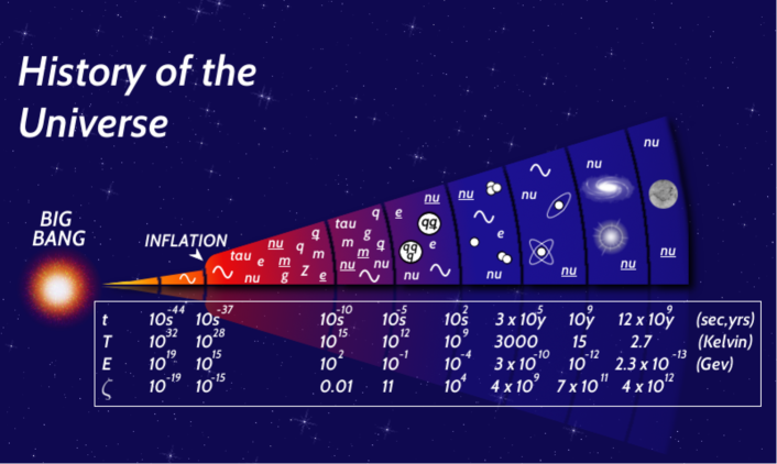
Figure 1: Sketch of the history of the universe as a function of time and temperature. As the universe evolves in time away from the big-bang, typical values of $\zeta$ for the proton change from about $10^{-19}$ at the Planck time to $10^{12}$ at the present day. Besides, a sequence of thermodynamic transitions takes place, starting from the electroweak transition ($\sim~{}10^{-9}~{}\rm s$), followed by the QCD transition ($\sim~{}10^{-6}~{}\rm s$) and by the $e^{+}e^{-}$ annihilation ($\sim~{}10^{2}~{}\rm s$) [35].

Relativistic Lattice Boltzmann schemes (usually referred to as Relativistic Lattice Boltzmann Methods (RLBMs) ) enter the game as a conceptual path to the construction of specific instances of kinetic models and as a computer-efficient numerical approach to the problem, meeting the obvious need of developing efficient and accurate numerical relativistic hydrodynamic solvers. These numerical tools are a clear must, as analytical methods suffer major limitations in describing complex phenomena which arise from strong nonlinearities and/or non-ideal geometries of direct relevance to experiments.

RLBMs have been developed in many variants starting from the beginning of the present decade and have emerged as a promising tool for the study of dissipative hydrodynamics in relativistic regimes. In this approach, the time evolution of the system is described by the one-particle distribution function, and macroscopic quantities are obtained as moments of this function.

The first model was developed by Mendoza et al. [18, 36] as an extension of the standard LB equation. The model is derived basing on Grad’s moment-matching technique and uses two different distribution functions, one for the particle number and one for energy and momentum.

Romatschke et al. [37] developed a scheme for an ultra-relativistic gas based on the expansion on orthogonal polynomials of the Maxwell-Jüttner distribution, following a procedure similar to the one used for non-relativistic LBM. This model is not compatible with a Cartesian lattice, thus requiring interpolation to implement the streaming phase, but has the advantage of supporting the description of systems in general space-time coordinates. Romatschke [38] has also shown that it is possible to extend the method to support non-ideal equations of state.

Li et al. [39] have extended the work of Mendoza et al. by using a multi relaxation-time collision operator. The model uses standard Cartesian lattices, and it is found that by independently tuning shear and bulk viscosity it is possible to cure numerical errors and discontinuities present in the original model. However, the model recovers only the first two moments of the distribution function, and does not allow accurate simulations of flows at large values of $\beta=u/c$, where $u$ is the fluid speed and $c$ the speed of light.

Mohseni et al. [40] have shown that it is possible to avoid multi-time relaxation schemes, still using a D3Q19 lattice and properly tuning the bulk viscosity for ultra-relativistic flows, so as to recover only the conservation of the momentum-energy tensor. This is a reasonable approximation in the ultra-relativistic regime, where the first order moment plays a minor role, but leaves open the problem of recovering higher order moments. A further step was taken in [41], with a relativistic lattice Boltzmann method (RLBM) able to recover higher order moments on a Cartesian lattice. This model provides an efficient tool for simulations in the ultra-relativistic regime in the Minkowski space-time.

All these developments use pseudo-particles of zero proper mass $m$. The extension of the model to account for massive particles was presented in [42], with the derivation of a unified scheme, allowing to conceptually bridge the gap between the ultra-relativistic regime ($\beta\simeq 1$), all the way down to the non-relativistic one ($\beta\rightarrow 0$).

Another significant algorithmic development was presented in [43], where the authors describe a systematic procedure to define quadrature rules at high orders, giving the possibility to go well beyond hydrodynamics and to handle flows from a strongly interacting near-inviscid regime, all the way to the ballistic regime. The model is restricted to flows of massless particles and has been so far applied only to one-dimensional flows. From a conceptual point of view, further extensions of this model could be of great interest to analyse the transition between hydrodynamic and non-hydrodynamic regimes in the framework of QGP.

Indeed QGP in possibly the most natural field of application for RLBM methods. In this context it has been used to investigate several problems of shock waves propagation [18, 36, 39, 44, 40, 41, 42, 45, 43] and other standard benchmarks, such as the 1-d Bjorken flow [37, 43, 46].

However, to the best of our knowledge, a fully-fledged implementation for simulating nuclear collisions has not been reported, as yet.

Another related application for RLBM is the theoretical study of relativistic transport coefficients. Based on RLBM simulations, recent works [45, 47, 48, 49] have reported an accurate analysis of the relativistic transport coefficients in the single-relaxation time approximation, presenting numerical evidence that the Chapman Enskog expansion accurately relates kinetic transport coefficients and macroscopic hydrodynamic parameters in dissipative relativistic fluid dynamics, confirming recent theoretical results.

Finally, several authors have attempted to adapt RLBM schemes to the study of $(2+1)$-dimensional relativistic hydrodynamics, motivated by the interest for the study of pseudo-relativistic systems such as the electrons flow in graphene. A series of theoretical works have taken into consideration the possibility of observing Rayleigh-Bénard instability [50, 51], Kelvin-Helmholtz instability [52], current whirlpools [53], as well as preturbulent regimes [54, 55] in a electronic fluid.

Most of these works and the results here summarized, have been based, with few exceptions, on formulations in three spatial dimensions with focus on the ultra-relativistic regime, in that they consider massless one-particle distribution functions; this is reflected at the macroscopic level by the emergence of an ultra-relativistic equation-of-state ($\epsilon=3P$, with $\epsilon$ the energy density and P the pressure). On the other hand, one would like to explore all kinematic regimes, as characterized by the dimensionless parameter

$$\zeta=\frac{mc^{2}}{k_{\rm B}T}\quad,$$ (1)

($m$ is a typical particle mass and $T$ a typical temperature). We shall make extensive reference to this parameter throughout the paper; while in many high-energy astrophysics contexts $\zeta\approx 0$, mildly relativistic regimes ($\zeta\approx 1\cdots 5$), which are typical of the QGP physics [56, 57, 11], indicate that ultra-relativistic treatments are not appropriate in this case. An interesting remark is that, as one follows the history of the Universe $\zeta$ gradually increases from $\zeta\approx 0$ towards $\zeta\rightarrow\infty$ (see Fig. 1).

Another important area is the study of low-dimensional systems, as it has been recently realised that “relativistic” fluid dynamics in $2d$ is relevant to the dynamics of electrons in graphene sheets or wider classes of $2d$ “exotic” materials governed, to a good approximation, by the dispersion relation $\epsilon_{\rm F}=v_{\rm F}|\bm{p}|$ (formally equivalent to that of a ultra-relativistic particle with $c$ replaced by the Fermi velocity $v_{\rm F}$).

A further open problem has been the lack of (conceptually and numerically)-accurate calibration procedures, relating the mesoscopic parameters (relaxation time) to the macroscopic transport coefficients e.g., shear and bulk viscosity and thermal conductivity.

The latter is not only a computational problem but a conceptual one as well, since the time-honored approaches to derive transport coefficients from the Boltzmann equation (such as Grad’s method and the Chapman-Enskog expansion, see later for details) yield different results in the relativistic regime.

These problems have been recently addressed in a series of papers [42, 45, 53, 49] that have: i) extended the kinematic regime from ultra-relativistic, all the way to near non-relativistic, using finite-mass pseudo-particles, ii) included the two-dimensional case as well and, iii) developed an accurate calibration procedure of the mesoscopic vs. macroscopic transport coefficients.

The present paper builds on these results and considerably extends them as follows: i) collects and summarizes in a structured way all the formal developments of early works; ii) extends algorithmic developments to in principle any number of spatial dimensions (in practice, $1\leq d\leq 3$) including external forcing as well, and using Gauss-type quadratures on space-filling Cartesian lattices, preserving the computational advantages of the classic LBM; iii) recasts early results in a more compact mathematical format; iv) extensively and accurately compares the relationship between mesoscopic and macroscopic transport coefficients in $1-2-3$ spatial dimensions, across all kinematic regimes, and finally, v) presents a wider set of validation benchmarks.

For validation purposes, we consider several flows in which approximate analytical solutions can be worked out and compared with numerical simulations based on the RLBMs described in this paper. In detail, we present results of simulations solving the Riemann problem for a quark-gluon plasma, showing good agreement with previous results obtained using other solvers present in the literature. We also present simulation results of laminar flows in ultra-clean graphene samples; we consider geometrical setups actually used in experiments, and provide numerical evidence of the formation of electron back-flows (“whirlpools”, in the jargon of graphene practitioners) in the proximity of current injectors.

3 Ideal Relativistic Hydrodynamics

In this section we introduce the hydrodynamic equations of an ideal relativistic fluid starting from the basic principles of relativistic kinetic theory, which will serve as the stepping stone for the derivation of the RLBM. A few fundamental references on the formulation of relativistic kinetic theory are the books by De Groot [8], Cercignani and Kremer [58], along with the recent monograph of Rezzolla and Zanotti [9] and the review by Paul and Ulrike Romatschke [10].

We consider an ideal non-degenerate relativistic fluid, consisting at the kinetic level of a system of interacting particles of mass $m$. The particle distribution function $f((x^{\alpha}),(p^{\alpha}))$, depending on space-time coordinates $\left(x^{\alpha}\right)=\left(ct,\bm{x}\right)$ and momenta $\left(p^{\alpha}\right)=\left(p^{0},\bm{p}\right)=\left(E/c,\bm{p}\right)$ ($c$ is the speed of light, $E$ the particle energy, with $E=cp^{0}=c\sqrt{|\bm{p}|^{2}+m^{2}c^{2}}$, and $\bm{x}$, $\bm{p}\in\mathbb{R}^{d}$), describes the probability of finding a particle with momentum $\bm{p}$ at a given time $t$ and position $\bm{x}$. We adopt Einstein’s summation convention over repeated indexes, and use Greek indexes to denote $(d+1)$ space-time coordinates and Latin indexes for $d$ dimensional spatial coordinates.

The particle distribution function obeys the relativistic Boltzmann equation, here taken in the Anderson-Witting [59, 60] relaxation-time approximation:

$$p^{\alpha}\frac{\partial f}{\partial x^{\alpha}}+mK^{\alpha}\frac{\partial f}{\partial p^{\alpha}}=\frac{U^{\alpha}p_{\alpha}}{\tau c^{2}}(f^{\rm eq}-f)\quad,$$ (2)

with $\tau$ the relaxation (proper-)time, $U^{\alpha}$ the macroscopic relativistic $(d+1)$-velocity (defined such that $U^{\alpha}U_{\alpha}=c^{2}$), and $K^{\alpha}$ the external forces acting on the system, assumed for simplicity not to depend on the momentum $(d+1)$-vector. The local equilibrium $f^{\rm eq}$ is given by the Maxwell-Jüttner distribution:

$$f^{\rm eq}=B(n,T)\exp{\left(-\frac{U^{\alpha}p_{\alpha}}{k_{\rm B}T}\right)}\quad,$$ (3)

with $k_{\rm B}$ the Boltzmann constant and $B$ a $d$-dependent normalization factor to be defined later in the text.

The Anderson-Witting model ensures the local conservation of particle number, energy and momentum, meaning that the particle four flow $N^{\alpha}$ and the energy momentum tensor $T^{\alpha\beta}$, defined respectively as the first and second moment of $f$

$$N^{\alpha} =c\int fp^{\alpha}\frac{\mathop{}\!\mathrm{d}^{d}p}{p_{0}}\quad,$$ (4)

$$T^{\alpha\beta} =c\int fp^{\alpha}p^{\beta}\frac{\mathop{}\!\mathrm{d}^{d}p}{p_{0}}\quad,$$ (5)

are conserved:

$$\partial_{\alpha}N^{\alpha} =0\quad,$$ (6)

$$\partial_{\beta}T^{\alpha\beta} =0\quad.$$ (7)

The conservation equations do not provide any dynamical property of the fluid until a specific decomposition of $N^{\alpha}$ and $T^{\alpha\beta}$ is specified. For an ideal fluid at the equilibrium it can be shown that

$$N^{\alpha}_{E}= ~{}nU^{\alpha}\quad,$$ (8)

$$T^{\alpha\beta}_{E}= ~{}\left(\epsilon+P\right)\frac{U^{\alpha}U^{\beta}}{c^{2}}-P\eta^{\alpha\beta}\quad,$$ (9)

where $\epsilon$ ($n$) is the energy (particle) density, $P$ the hydrostatic pressure and $\eta^{\alpha\beta}$ the Minkowski metric tensor. In the following we will use $\eta^{\alpha\beta}=diag(1,-\mathds{1})$, with $\mathds{1}=\left(1,\dots,1\right)\in\mathbb{N}^{d}$.

The closure for the conservation equations is given by an appropriate Equation of State (EOS). In order to derive the EOS for a perfect gas in $(d+1)$ space-time coordinates in a relativistic regime, we first define the normalization factor $B(n,T)$ in Eq. 3 in order to satisfy the constraint given by Eq. 8. Therefore we write:

$$c\int f^{\rm eq}p^{\alpha}\frac{\mathop{}\!\mathrm{d}^{d}p}{p_{0}}=cB\int e^{-\frac{p_{\mu}U^{\mu}}{k_{\rm B}T}}p^{\alpha}\frac{\mathop{}\!\mathrm{d}^{d}p}{p_{0}}=c~{}B~{}Z^{\alpha}=nU^{\alpha}\quad,$$ (10)

and together with the analytical expression for the integral $Z^{\alpha}$ (see Appendix B for details), we can determine the correct normalization factor for the equilibrium distribution function

$$B(n,T)=\left(\frac{c}{k_{\rm B}T}\right)^{d}\frac{n}{2^{\frac{d+1}{2}}\pi^{\frac{d-1}{2}}\zeta^{\frac{d+1}{2}}K_{\frac{d+1}{2}}(\zeta)}\quad;$$ (11)

the relativistic parameter $\zeta=\frac{mc^{2}}{k_{\rm B}T}$ has been already defined in the previous section, and $K_{i}(\zeta)$ is the modified Bessel function of the second kind of index $i$. Next, we take the definition of the momentum-energy tensor (Eq. 5), and use the normalization factor $B(n,T)$ together with the analytical expression for $Z^{\alpha\beta}$ (see again Appendix B), giving

$$c\int f^{\rm eq}p^{\alpha}p^{\beta}\frac{\mathop{}\!\mathrm{d}^{d}p}{p_{0}}=c~{}B~{}Z^{\alpha\beta}=PG_{d}\frac{U^{\alpha}U^{\beta}}{c^{2}}-nk_{\rm B}T\eta^{\alpha\beta}\quad,$$ (12)

where we have introduced the dimensionless parameter

$$G_{d}=\frac{\epsilon+P}{P}=\zeta\frac{K_{\frac{d+3}{2}}(\zeta)}{K_{\frac{d+1}{2}}(\zeta)}\quad.$$ (13)

In order to identify the equation of state it is sufficient to match the terms with the same tensor structure in Eq. 12 and Eq. 9; one finally obtains:

$$\begin{array}[]{rll}\epsilon&=&P\left(G_{d}-1\right)\quad,\\ P&=&nk_{\rm B}T\quad.\end{array}$$ (14)

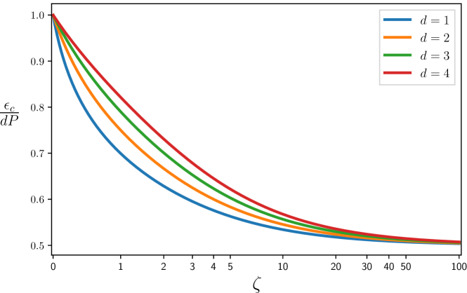
Figure 2: Ratio of kinetic energy density (normalized on the number of spatial dimensions $d$) and pressure for an ideal gas. For better readability the coordinate on the horizontal axis is rescaled as $\zeta\rightarrow\log(\zeta+\sqrt{1+\zeta^{2}})$. The correct limiting value for kinetic energy density is recovered both in the classical and in the ultra-relativistic regime.

For example, in $(3+1)$ dimensions we have:

$$\begin{array}[]{rll}\epsilon&=&P\left(\zeta\frac{K_{3}(\zeta)}{K_{2}(\zeta)}-1\right)=P\left(3+\zeta\frac{K_{1}(\zeta)}{K_{2}(\zeta)}\right)\quad.\\ P&=&nk_{\rm B}T\quad.\end{array}$$ (15)

a result already derived many years ago [61].

It is interesting to look at the asymptotic behaviour of Eq. 14: it is simple to show that taking the limit $\zeta\rightarrow 0$, for which $G_{d}\rightarrow d+1$, we obtain the well known ultra-relativistic EOS:

$$\epsilon_{\rm ur} =dP\quad.$$ (16)

For the non-relativistic limit we define the kinetic energy density $\epsilon_{c}=\epsilon-n~{}mc^{2}$ and take the limit for $\zeta\rightarrow\infty$ . Using the fact that $(x~{}K_{\alpha}(x)/K_{\alpha-1}(x)-x)\rightarrow\alpha-1/2$ as $x\rightarrow\infty$ one recovers the well known non-relativistic expression for the EOS of an ideal gas:

$$\epsilon_{c} =\frac{d}{2}P\quad.$$ (17)

Finally, Fig. 2 plots the ratio of kinetic energy divided by pressure (and rescaled by the number of spatial dimensions) for several values of $d$ and in a wide kinematic range, showing a continuous crossover from the ultra-relativistic to the classical regimes.

From the EOS it is straightforward to derive a few thermodynamic quantities (see e.g. [58] for their formal definition) which will be useful in the coming sections, such as the heat capacity at constant volume $c_{v}$:

$$c_{v}=\frac{\partial(\epsilon/n)}{\partial T}=k_{\rm B}\left[(2+d)G_{d}+\zeta^{2}-G_{d}^{2}-1\right]\quad,$$ (18)

the heat capacity at constant pressure $c_{P}$ ( $h_{e}=(\epsilon+P)/n$ is the relativistic enthalpy per particle) :

$$c_{P}=\frac{\partial h_{e}}{\partial T}=k_{\rm B}\left[(2+d)G_{d}+\zeta^{2}-G_{d}^{2}\right]\quad,$$ (19)

and the adiabatic sound speed $c_{s}$:

$$c_{s}=c\sqrt{\frac{P}{\epsilon+P}\frac{c_{p}}{c_{v}}}=c\sqrt{\frac{(2+d)G_{d}+\zeta^{2}-G_{d}^{2}-1}{G_{d}\left((2+d)G_{d}+\zeta^{2}-G_{d}^{2}\right)}}\quad.$$ (20)

4 Dissipative Effects and Transport Coefficients

When dissipative effects are taken into account, the definition of the non-equilibrium component of $N^{\alpha}$ and $T^{\alpha\beta}$ is ambiguous as it depends on the choice of the local rest frame, with the two most common choices being the one suggested by Eckart [3] and by Landau and Lifshitz [5]. The Anderson-Witting model is based on the Landau-Lifshitz decomposition, where the fluid velocity $U^{\alpha}$ is defined such as to satisfy

$$T^{\alpha\beta}U_{\beta}=\epsilon~{}U^{\alpha}\quad,$$ (21)

and for which, assuming a linear combination of the contribution due to the equilibrium and the non-equilibrium part, it follows that

$$N^{\alpha} =N^{\alpha}_{E}-\frac{1}{h_{e}}q^{\alpha}\quad,$$ (22)

$$T^{\alpha\beta} =T^{\alpha\beta}_{E}-\varpi\Delta^{\alpha\beta}+\pi^{<\alpha\beta>}\quad,$$ (23)

where $q^{\alpha}$ is the heat flux, $\pi^{<\alpha\beta>}$ the pressure deviator, $\varpi$ the dynamic pressure, and

$$\Delta^{\alpha\beta}=\eta^{\alpha\beta}-\frac{1}{c^{2}}U^{\alpha}U^{\beta}\quad,$$ (24)

is the (Minkowski-)orthogonal projector to the fluid velocity $U^{\alpha}$ (see Appendix A for complete definition of all tensorial objects that we use and [58] for a full treatment of the problem).

The non-equilibrium contribution to $N^{\alpha}$ and $T^{\alpha\beta}$ can be used to define the transport coefficients which enter the linear relations between thermodynamic forces and fluxes:

$$q^{\alpha} =\lambda\left(\nabla^{\alpha}T-\frac{T}{nh_{e}}\nabla^{\alpha}P\right)\quad,$$ (25)

$$\pi^{<\alpha\beta>} =\eta\left(\Delta^{\alpha}_{\gamma}\Delta^{\beta}_{\delta}+\Delta^{\alpha}_{\delta}\Delta^{\beta}_{\gamma}-\frac{1}{d}\Delta^{\alpha\beta}\Delta_{\gamma\delta}\right)\nabla^{\gamma}U^{\delta}\quad,$$ (26)

$$\varpi =-\mu\nabla_{\alpha}U^{\alpha}\quad;$$ (27)

$\lambda$ is the thermal conductivity, $\eta$ and $\mu$ the shear and bulk viscosities, and we have used the shorthand notation

$$\begin{array}[]{lcl}\nabla^{\alpha}&=&\Delta^{\alpha\beta}\partial_{\beta}\quad,\\ \Delta^{\alpha}_{\beta}&=&\Delta^{\alpha\gamma}\Delta_{\gamma\beta}\quad.\end{array}$$ (28)

The transport coefficients provide the link between the kinetic and the macroscopic layer. In non-relativistic regimes, the derivation of appropriate transport coefficients is typically obtained with either Grad’s method of moments [62] or the Chapman-Enskog (CE) expansion [63]; both techniques provide a consistent connection between kinetic theory and hydrodynamics, i.e. they provide the same expressions for the transport coefficients. However, it is well known that the two methods give different results in the relativistic regime.

In recent times, the problem has been extensively studied. Theoretical works and numerical investigations seem to converge towards the results provided by the CE approach but the question is still open to debate.

Here we consider both the CE and Grad’s method of moments expansion in a general $(d+1)$ space-time coordinate system, deriving all transport coefficients for the relativistic Boltzmann equation in the RTA. Derivations of some of these coefficients have appeared sparsely in the literature, often for specific quantities and specific space dimensions [27, 19, 64, 30, 65, 66, 67, 68, 69, 70, 71]. For this reason, we consider it useful to gather here for reference the full set of results using both approaches. We follow closely the procedure presented in [58] for the $(3+1)$-dimensional case. In the following we review the procedure used to derive these results, with full details and results collected in Appendix C.

4.1 Chapman-Enskog expansion

The Chapman-Enskog expansion consists in splitting the particle distribution function $f$ in two additive terms: the equilibrium distribution $f^{\rm eq}$ and a non equilibrium part $f^{\rm neq}$. When working in a hydrodynamic regime, it is reasonable to approximate $f^{\rm neq}$ with a small deviation from the equilibrium:

$$f=f^{\rm eq}+f^{\rm neq}\sim f^{\rm eq}(1+\phi)\quad.$$ (29)

with $\phi$ of the order of the Knudsen number $\rm Kn$, defined as the ratio between the mean free path and a typical macroscopic length scale. The general idea is to determine an analytical expression for the deviation from the equilibrium $f^{\rm eq}\phi$. We start from Eq. 2 (let us ignore for the moment the forcing term), insert Eq. 29 and retain only terms $\mathcal{O}(\rm{Kn})$, giving:

$$p^{\alpha}\frac{\partial f^{\rm eq}}{\partial x^{\alpha}}=-\frac{p^{\alpha}U_{\alpha}}{c^{2}\tau}f^{\rm eq}\phi\quad.$$ (30)

To derive the transport coefficients one then proceeds with the following steps:

1. Compute the derivative $p^{\alpha}\partial_{\alpha}f^{\rm eq}$ and derive the constitutive equations of a relativistic Eulerian fluid.

2. Use the balance equations for energy and momentum to eliminate the convective time derivatives and derive the analytic expression of $\phi$.

3. Use the now known expression for $f^{\rm eq}\phi$ to compute the first and second order tensors (via their integral definitions), compare against their definition in the Landau frame and work out the expression for the transport coefficients.

See Appendix C for a full discussion and full analytical expressions in an arbitrary number of space dimensions. Here we only mention the ultra-relativistic limit:

$$\lambda_{\rm ur} =\frac{d+1}{d}c^{2}k_{\rm B}n\tau\quad,$$ (31)

$$\mu_{\rm ur} =0\quad,$$ (32)

$$\eta_{\rm ur} =\frac{d+1}{d+2}P\tau\quad.$$ (33)

4.2 Grad’s moments method

The starting point for the derivation of Grad’s method of moments is similar to that of the Chapman Enskog expansion, with the splitting of the particle distribution function into two terms, the equilibrium and the non-equilibrium part. The way the non-equilibrium part is derived is however significantly different; while CE makes use of a small parameter of the order of the Knudsen number, Grad’s method is based on the expansion of the distribution function onto a set of orthonormal basis functions. The expansion is then truncated, setting to zero the kinetic moments beyond a prescribed order. When applying this formalism in the non-relativistic framework, the expansion is based on the Hermite polynomials, since their projection coefficients deliver the kinetic moments of the distribution function. In Appendix F we define a set relativistic polynomials having this same property, which we will use as the expansion basis for Grad’s method. It is important to stress that this approach, which was also used in the 14-moment approximation of Israel-Stewart, presents significant pitfalls which have been identified and corrected by Denicol et al [19]. In particular these authors have shown the importance of using a irreducible set of tensors, such as for example $\{1,\Delta^{\alpha\beta}p_{\beta},p^{<\alpha}p^{\beta>},\dots\}$. For these reasons, we remark that the procedure sketched here (and described in full details in Appendix C) should be improved as described in Ref. [19], and extended to an arbitrary number of space dimensions.

We start giving the definition of the entropy density $s$:

$$s=-\frac{k_{\rm B}}{nc}U^{\alpha}\int p_{\alpha}f\ln{f}\frac{d^{d}p}{p_{0}}\quad.$$ (34)

The derivation, constrained to the maximization of $s$, can be summarized in the following steps:

1. Using Lagrange multipliers method, find an expansion for $f$ that extremizes the entropy density $s$, with the constraints given by definition of $N^{\alpha}U_{\alpha}$, $U_{\alpha}T^{\alpha\beta}$ and $U_{\alpha}T^{\alpha<\beta\gamma>}$ (see Appendix C).

2. Using Grad’s ansatz for $f$ we compute the third order moment $T^{\alpha\beta\gamma}$.

3. The above expression is then plugged into Eq. 2 to determine the non-equilibrium components of the energy-momentum tensor.

4. By applying appropriate projectors it is then possible to derive the constitutive equations for the heat-flux, dynamic pressure and the pressure deviator. The expressions for the transport coefficients are derived by comparison with Eq. 25, Eq. 26, and Eq. 27.

Once again, detailed derivations and results are collected in Appendix C; in the ultra-relativistic limit we have:

$$\lambda_{\rm ur} =\frac{d+1}{d+2}c^{2}k_{\rm B}n\tau\quad,$$ (35)

$$\mu_{\rm ur} =0\quad,$$ (36)

$$\eta_{\rm ur} =\frac{d+1}{d+3}P\tau\quad.$$ (37)

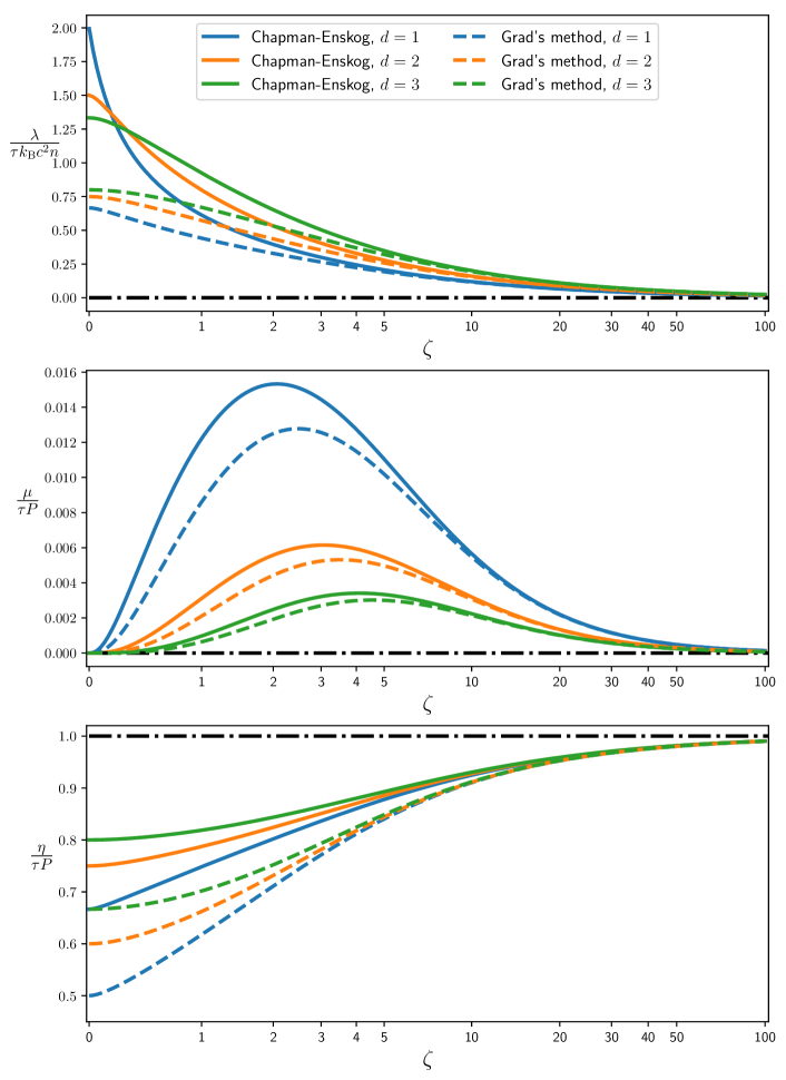
Figure 3: Comparison of the non-dimensional thermal conductivity, shear and bulk viscosity in $1,2,3$-dimensions, obtained applying the Chapman-Enskog expansion and Grad’s method of moments to the relativistic Boltzmann equation in the relaxation time approximation. The black dotted line represents the limit for $d\rightarrow\infty$; this result is the same using both CE and Grad’s method, and shows that in this limit all transport coefficients are classical.

As already remarked, the two methods give different results for the values of all transport coefficients, even if they tend to agree as one approaches the non relativistic regime. This is clearly shown in Fig. 3 where the behavior of $\eta$, $\mu$ and $\lambda$, as predicted by the two approaches, is shown as a function of $\zeta$. Lacking any realistic option for experimental verification, we will see in later sections that our numerical experiments strongly point to the CE approach. A mathematically nice result (although of little interest for physical purposes) is that, in the limit of an infinite number of spatial dimensions, all coefficients remain constant at their non relativistic value over the full kinematic range.

Finally, the behavior of the thermal conductivity needs a further explanation. It is well known, and it can directly be seen from Eq. 25, that the heat flux present a significant difference between the relativistic and the non-relativistic form; indeed for a relativistic iso-thermal fluid there could be a non-zero heat-flux due to a pressure gradient. Looking at Fig. 3 one may be puzzled as $\lambda$ seems to go to $0$ in the non-relativistic limit. This is so because, for later convenience, we plot $\frac{\lambda}{\tau k_{B}c^{2}n}$. If one recasts the expression as $\frac{\lambda m}{k_{\rm B}P\tau}$ and considers the limit for large $\zeta$, one obtains

$$\lambda=\frac{k_{\rm B}}{m}P\tau\left(\frac{d+2}{2}-\frac{3(d+2)}{2\zeta}+\dots\right)\quad,$$ (38)

whose first term is the well-known non-relativistic value.

5 Relativistic Lattice Boltzmann Methods

In recent times, numerical schemes based on the Lattice Boltzmann Method (LBM) have emerged as a promising tool for the study of dissipative relativistic hydrodynamics [18, 37, 38, 41, 42, 43, 47]. The advantage of this approach is that by working at a mesoscopic level viscous effects are naturally included, with relativistic invariance and causality preserved by construction.

In this section we present in full details the algorithmic extension of the LBM to the study of relativistic fluids, describing the derivation of a model which allows to cover a wide range of relativistic regimes, in principle all the way from fluids of ultra-relativistic massless particles down to non-relativistic fluids.

5.1 From continuum to the lattice

We here outline the procedure followed to derive the relativistic lattice Boltzmann equation, following a procedure similar to the one used with non-relativistic [72, 73, 74, 75] and earlier ultra-relativistic LBMs [37, 41]. In this section, we use natural units, $c=k_{\rm B}=1$, which helps write many formulas in a more compact form.

1. We start by writing Eq. 2 in terms of quantities that can be discretized on a regular lattice, by dividing the left and right hand sides by $p^{0}$:

   $$\partial_{t}f+v^{i}\nabla_{i}f=\frac{U^{\alpha}p_{\alpha}}{\tau p^{0}}(f^{\rm eq}-f)-\frac{mK^{\alpha}}{p^{0}}\frac{\partial f}{\partial p^{\alpha}}\quad,$$ (39)

   with $v^{i}=p^{i}/p^{0}$ the components of the microscopic velocity. In Eq. 39 the time-derivative and the propagation term are the same as in the non-relativistic regime; the price to pay is an additional dependence on $p^{0}$ of the relaxation (and forcing) term.

2. Next, we expand $f^{\rm eq}$ in an orthogonal basis; we adopt Cartesian coordinates and use a basis of polynomials orthonormal with respect to a weight $\omega(p^{0})$ given by the Maxwell-Jüttner distribution in the fluid rest frame (where $U^{i}=0$).

   Following a Gram-Schmidt procedure one then derives a set of polynomials $\{J^{(i)},i=1,2\dots\}$, which are used to build the expansion:

   $$f^{\rm eq}((p^{\mu}),(U^{\mu}),T)=\omega(p^{0})\sum_{k=0}^{\infty}a^{(k)}((U^{\mu}),T)J^{(k)}((p^{\mu}))\quad,$$ (40)

   where $a^{(k)}$ are the projection coefficients defined as

   $$a^{(k)}((U^{\mu}),T)=\int f^{\rm eq}((p^{\mu}),(U^{\mu}),T)J^{(k)}((p^{\mu}))\frac{\mathop{}\!\mathrm{d}^{d}p}{p^{0}}\quad.$$ (41)

   The polynomials are derived in such a way that the coefficients $a^{(k)}$ coincide by construction with the moments of the distribution function; as a result the quantity $f_{N}^{\rm eq}((p^{\mu}),(U^{\mu}),T)$, obtained truncating the summation in Eq. 40 to $N$, correctly preserves the moments of the distribution up to the $N$-th order. Observe that until now the discussion holds its validity in the continuum.

3. We now find a Gauss-like quadrature on a regular Cartesian grid able to reproduce correctly the moments of the original distribution up to order $N$. We proceed in such a way as to preserve exact streaming, meaning that all quadrature points $v^{l}_{i}=p^{l}_{i}/p^{0}$ must sit on lattice sites. At this point, the discrete version of the equilibrium function reads as follows:

   $$f_{iN}^{\rm eq}=w_{i}\sum_{k}a^{(k)}((U^{\mu}),T)J^{(k)}((p^{\mu}_{i}))\quad,$$ (42)

   with $w_{i}$ appropriate weights, $(p^{\mu}_{i})$ the linked abscissae, and the summation running on the total number of orthogonal polynomials up to the order $N$.

4. Once a quadrature rule is defined, it is possible to write down the discrete relativistic Boltzmann equation:

   $$f_{i}(\bm{x}+\bm{v}^{i}\Delta t,t+\Delta t)-f_{i}(\bm{x},t)=\Delta t~{}\frac{p_{i}^{\alpha}U_{\alpha}}{p^{0}_{i}\tau}(f_{i}^{\rm eq}-f_{i})+F^{\rm ext}_{i}\quad,$$ (43)

   where $F^{\rm ext}_{i}$ is the discretization of the total external forces acting on the system, more details will be given in Section 5.4.

5.2 Polynomial expansion of the equilibrium distribution function

In this section we define the polynomial expansion of the Maxwell-Jüttner distribution in $(d+1)$-dimensions. It turns out that using non-dimensional quantities is very useful here; to this purpose, we introduce a reference temperature $T_{0}$ (and a corresponding energy scale $k_{B}T_{0}$) and define the following quantities: $\tilde{T}=T/T_{0}$, $\tilde{m}=mc^{2}/(k_{B}T_{0})$, $\tilde{p}^{\alpha}=cp^{\alpha}/(k_{B}T_{0})$. $T_{0}$ is in principle arbitrary; we will see in the following that $T_{0}$ is needed to translate between lattice and physical units; for the moment the reader may consider $T_{0}$ as a typical temperature/energy scale of the system under study.

We start by constructing a set of polynomials in the variables $\tilde{p}^{\alpha}$, orthogonal with respect to a weighting function given by the equilibrium distribution in the co-moving frame:

$$\omega(p^{0},T_{0})=C(\tilde{m},T_{0})\exp{\left(-\tilde{p}^{0}\right)}\quad;$$ (44)

$C$ is a normalization factor, which deserves a further remark: while the normalization factor $B(n,T)$ in Eq. 3 carries an important physical meaning (as discussed in Section 3), $C$ can be chosen in the most expedient way. In most cases we will find it convenient to take the normalization factor $C$ such to satisfy the condition

$$\int\omega(p^{0},T_{0})\frac{\mathop{}\!\mathrm{d}^{d}p}{p^{0}}=(\frac{k_{B}T_{0}}{c})^{d-1}\int\omega(p^{0},T_{0})\frac{\mathop{}\!\mathrm{d}^{d}\tilde{p}}{\tilde{p}^{0}}=1\quad,$$ (45)

implying

$$C(\tilde{m},T_{0})=\frac{1}{2^{\frac{d+1}{2}}\pi^{\frac{d-1}{2}}\tilde{m}^{\frac{d-1}{2}}K_{\frac{d-1}{2}}\left(\tilde{m}\right)}~{}\frac{c}{k_{B}T_{0}^{d-1}}\quad.$$ (46)

Starting from the set $\mathcal{V}=\{1,\tilde{p}^{\alpha},\tilde{p}^{\alpha}\tilde{p}^{\beta},\dots\}$ we apply the Gram-Schmidt procedure to derive the polynomials up to a desired order. We label the polynomials with the notation $J^{(n)}_{\alpha_{1}\cdots\alpha_{n}}$, where $n$ is the order of the polynomial and the $\alpha$ indexes corresponds to the components of $(\tilde{p}^{\alpha})$ they depend upon. All integrals needed to carry out this procedure are computed in Appendix B. The first polynomials (up to order $1$) in $(d+1)$ dimensions are easily written:

$$J^{(0)} =1\quad,$$

$$J^{(1)}_{0} =\frac{\tilde{p}^{0}-\tilde{G}_{d-2}}{\sqrt{\tilde{m}^{2}-\tilde{G}_{d-2}^{2}+d\tilde{G}_{d-2}}}\quad,$$

$$J^{(1)}_{i} =\frac{\tilde{p}^{i}}{\sqrt{\tilde{G}_{d-2}}}\quad;$$

here we use the shorthand notation $\tilde{G}_{d-2}=G_{d-2}(\tilde{m})$, with $G_{d}$ defined in Eq. 13. Their ultra-relativistic limit is given by:

$$J^{(0)} =1\quad,$$

$$J^{(1)}_{0} =\frac{\tilde{p}^{0}}{\sqrt{d-1}}-\sqrt{d-1}\quad,$$

$$J^{(1)}_{i} =\frac{\tilde{p}^{i}}{\sqrt{d-1}}\quad.$$

The corresponding projection coefficients (defined through 41 and taking into account the normalization of $f^{\rm eq}$ given by Eq. 11) are given by:

$$a^{(0)} =\frac{cn}{k_{B}T_{0}}~{}\frac{1}{G_{d-2}\tilde{T}}\quad,$$

$$a^{(1)}_{0} =\frac{cn}{k_{B}T_{0}}~{}\left(U^{0}-\frac{\tilde{G}_{d-2}}{\tilde{T}G_{d-2}}\right)\frac{1}{\sqrt{\tilde{m}^{2}+\tilde{G}_{d-2}(d-\tilde{G}_{d-2})}}\quad,$$

$$a^{(1)}_{i} =\frac{cn}{k_{B}T_{0}}~{}\frac{U^{i}}{\sqrt{\tilde{G}_{d-2}}}\quad;$$

where $G_{d-2}$ (as opposed to $\tilde{G}_{d-2}$) is again a shorthand for $G_{d-2}=G_{d-2}(m/T)\equiv G_{d-2}(\tilde{m}/\tilde{T})$. The ultra-relativistic limit reads:

$$a^{(0)} =\frac{cn}{k_{B}T_{0}}~{}\frac{1}{(d-1)\tilde{T}}\quad,$$

$$a^{(1)}_{0} =\frac{cn}{k_{B}T_{0}}~{}\left(\frac{U^{0}}{\sqrt{d-1}}-\frac{1}{\tilde{T}\sqrt{d-1})}\right)\quad,$$

$$a^{(1)}_{i} =\frac{cn}{k_{B}T_{0}}~{}\frac{U^{i}}{\sqrt{d-1}}\quad.$$

Having derived both the polynomials and the projections we can then write down the first order expansion version of the Maxwell-Jüttner distribution in $(d+1)$-dimension:

$$f^{\rm eq} =\frac{cn}{k_{B}T_{0}}~{}\omega(\tilde{p}^{0})\left(\frac{1}{G_{d-2}\tilde{T}}+\frac{(\tilde{p}^{0}-\tilde{G}_{d-2})}{\tilde{G}_{d-2}(d-\tilde{G}_{d-2})+\tilde{m}^{2}}\left(U^{0}-\frac{\tilde{G}_{d-2}}{\tilde{T}G_{d-2}}\right)-\frac{1}{\tilde{G}_{d-2}}p^{i}U_{i}\right)\quad.$$

The expression in the ultra-relativistic limit is slightly simpler:

$$f^{\rm eq} =\frac{cn}{k_{B}T_{0}}~{}\omega(\tilde{p}^{0})~{}\frac{d/\tilde{T}+U^{0}\tilde{p}^{0}-(d-1)U^{0}-\tilde{p}^{i}U_{i}}{d-1}\quad.$$

Expressions at higher orders are rather bulky and are therefore given as supplementary material [76]. Here we only stress the general structure of the expansion:

• all polynomials are adimensional and written in terms of $\tilde{p}^{\alpha}$ and of $\tilde{m}$;

• all expansion coefficients are the product of $\frac{cn}{k_{B}T_{0}}$ and again an adimensional expression, that depends on $U^{\alpha}$, $\tilde{T}$ and $\tilde{m}$;

• the resulting expressions for $f^{\rm eq}$ are again the product of $\frac{cn}{k_{B}T_{0}}$ and an adimensional expression.

This structure will make it very simple to relate lattice-defined quantities with the corresponding physical ones. See later on this point.

Fig. 4 shows the expansion of $f^{\rm eq}$ up to the fifth order in $(2+1)$ dimensions in the massless limit and compares with the analytical expression. $f^{\rm eq}$ is plotted as a function of $\bm{\tilde{p}}=(\tilde{p}_{x},0)$ with $n$, $\tilde{T}$ and $T$ all equal to unity and $\beta=|U^{i}|/U^{0}=0.5$.

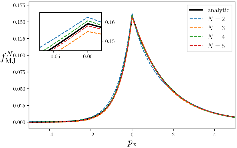
Figure 4: Comparison of the analytic Maxwell Jüttner distribution in $(2+1)$ dimensions against approximations at various orders $N$, computed using an orthogonal polynomial basis. The distributions are shown as functions of $\bm{p}=(p_{x},0)$, having fixed all the other parameters to $\tilde{m}=0$, $\tilde{T}=1$, $n=1$ and $\beta=|U^{i}|/U^{0}=0.5$.

The massless limit in $(1+1)$ dimensions needs special care, as the normalization factor of $\omega(p^{0},T_{0})$ defined by Eq. 46 is in this case proportional to $1/K_{0}(\tilde{m})$ and diverges when $\tilde{m}\rightarrow 0$, so the weighting function is ill-defined. In this case, in order to define a valid kernel for the Gram-Schmidt procedure, we use for $\omega(p^{0},T_{0})$ a normalization factor analogous to the one defined in Eq. 11, that, in this case, writes

$$C(\tilde{m},T_{0})=\frac{c}{k_{B}T_{0}}\frac{1}{2\tilde{m}K_{1}(\tilde{m})}\quad.$$ (47)

We denote with $\mathcal{J}^{(n)}_{\alpha_{1}\cdots\alpha_{n}}$ the polynomials derived starting from the above defined weighting function, which up to order $1$ take the following form:

$$\mathcal{J}^{(0)} =\frac{1}{\sqrt{\frac{\tilde{G}_{1}-2}{\tilde{m}^{2}}}}\quad,$$

$$\mathcal{J}^{(1)}_{0} =\frac{\tilde{p}^{0}}{\sqrt{-\frac{\tilde{m}^{2}}{\tilde{G}_{1}-2}+\tilde{G}_{1}-1}}-\frac{\tilde{m}^{2}}{\left(\tilde{G}_{1}-2\right)\sqrt{-\frac{\tilde{m}^{2}}{\tilde{G}_{1}-2}+\tilde{G}_{1}-1}}\quad,$$

$$\mathcal{J}^{(1)}_{i} =\tilde{p}^{i}\quad.$$

For the projections, we have:

$$\mathcal{A}^{(0)} =\frac{n}{T_{0}}\frac{(G_{1}-2)\tilde{T}}{\tilde{m}^{2}\sqrt{\frac{\tilde{G}_{1}-2}{\tilde{m}^{2}}}}\quad,$$

$$\mathcal{A}^{(1)}_{0} =\frac{n}{T_{0}}\frac{U^{0}}{\sqrt{-\frac{\tilde{m}^{2}}{\tilde{G}_{1}-2}+\tilde{G}_{1}-1}}-\frac{(G_{1}-2)\tilde{T}}{\left(\tilde{G}_{1}-2\right)\sqrt{-\frac{\tilde{m}^{2}}{\tilde{G}_{1}-2}+\tilde{G}_{1}-1}}\quad,$$

$$\mathcal{A}^{(1)}_{i} =\frac{n}{T_{0}}U^{i}\quad.$$

One may now check that while independent limits of polynomials and projections are still divergent, the limit of the product of each polynomial with its corresponding projection is convergent also in the massless limit; the limiting value for $f_{N}^{\rm eq}((\tilde{p}^{\mu}),(U^{\mu}),\tilde{T})$ is then well-behaved:

$$f_{N}^{\rm eq}((\tilde{p}^{\mu}),(U^{\mu}),\tilde{T})=\omega(p^{0},T_{0})\sum_{k=0}^{N}\lim_{\tilde{m}\rightarrow 0}\left(a^{(k)}((U^{\mu}),\tilde{T})J^{(k)}((\tilde{p}_{i}^{\mu}))\right)\quad.$$ (48)

Up to first order, one obtains:

$$f^{\rm eq}=\frac{cn\omega(\tilde{p}_{0})}{k_{B}T_{0}}\left[\frac{1-\tilde{p}^{0}}{\tilde{T}}+\tilde{p}^{0}U^{0}+\tilde{p}^{x}U^{x}\right]$$ (49)

This expression has the same structure as for the general case that we have discussed before. Note however, that the fact that polynomials and projections do not have independent finite limits in the massless case will require special care for the construction of Gaussian quadratures.

5.3 Gauss-type quadratures with prescribed abscissas

The discrete formulation of the theory discussed above is based on a Gauss-type quadrature on a Cartesian grid. As we move onto this discrete lattice, from now on we use natural units ($c=1$ and $k_{B}=1$) allowing to write down mathematically slimmer expressions; as ultimately all grid-defined quantities are adimensional, any specific choice on the preferred dimensional units will only affect the conversion factors between physical and numerical units (see later for details).

In order to ensure that all quadrature points lie on lattice sites, and to preserve the moments of a distribution up to a desired order $N$, we need to determine the weights and the abscissas of a quadrature such to satisfy the orthonormal conditions [77]:

$$\int\omega(p^{0},T_{0})J_{l}^{(m)}((\tilde{p}^{\mu}))J_{k}^{(n)}((\tilde{p}^{\mu}))\frac{\mathop{}\!\mathrm{d}^{d}\tilde{p}}{\tilde{p}^{0}}=\sum_{i}w_{i}J_{l}^{(m)}((\tilde{p}^{\mu}_{i}))J_{k}^{(n)}((\tilde{p}^{\mu}_{i}))=\delta_{lk}\delta_{mn}\quad,$$ (50)

with $(\tilde{p}^{\mu}_{i})$ the discrete $(d+1)$ momentum vectors. A convenient parametrization of $(\tilde{p}^{\mu}_{i})$ writes as follows:

$$(\tilde{p}^{\mu}_{i})=p^{0}_{i}(1,v_{0}n_{i})\quad,$$ (51)

where $n_{i}\in\mathbb{Z}^{d}$ are the vectors forming the stencil $G=\{n_{i}~{}|~{}i=1,2,\dots,i_{max}\}$ defined by the (on-lattice) quadrature points, $v_{0}$ is a free parameter that can be freely chosen such that $v_{i}=v_{0}||n_{i}||<1,\forall i$, and $\tilde{p}_{i}^{0}$ is defined as

$$\tilde{p}_{i}^{0}=\tilde{m}\gamma_{i}=\tilde{m}\frac{1}{\sqrt{1-|v_{i}|^{2}}}\quad.$$ (52)

In order to determine a quadrature we proceed as follows: i) select a specific value for $\tilde{m}$, ii) choose a set of velocity vectors $G$, containing a sufficient number of elements such that the left hand side of Eq. 50 is a full ranked matrix, iii) look for a solution of Eq. 50 formed by non-negative weights $(w_{i}\geq 0,\forall i)$.

Observe that while the parametrization in Eq. 51 is general and can be used to determine quadratures for wide ranges of values of $\tilde{m}$, the limit case of massless particles requires a slightly different approach, as Eq. 52 is not well defined for $\tilde{m}=0$; in this case we let $\tilde{p}^{0}_{i}$ be free parameters (as already suggested in [41]) to be determined such as to satisfy Eq. 50. We can have several energy shells associated to each vector and therefore we add a second index to Eq. 51:

$$\left(\tilde{p}^{\mu}_{i,j}\right)=\tilde{p}^{0}_{j}\left(1,\frac{n_{i}}{||n_{i}||}\right)\quad,$$ (53)

where the index $j$ labels different energy shells, and $||n_{i}||$ has to be the same for all the stencil vectors since all particles travel at the same speed $v_{i}=c=1,\forall i$. Examples of stencils in $2d$ for the massive and massless case are shown in Fig. 5.

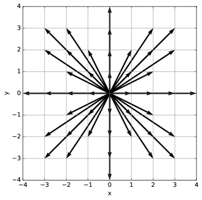
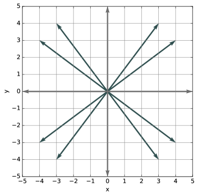
Figure 5: Two examples of stencil compatible with a third order quadrature, respectively for $\tilde{m}=5$ (left) and $\tilde{m}=0$ (right). The points forming the stencil for $\tilde{m}=0$ lie on the intersection between the Cartesian grid and a circle of radius $5$.

As a concrete example, we consider the $(2+1)$ dimensional case and solve Eq. 50 with $\{J^{(i)},i=1,2\dots\}$ the orthogonal polynomials in Appendix F, $(\tilde{p}^{\mu}_{i})$ the three-momentum vectors following the parametrization in Eq. 51 and $w_{i}$ suitable weights. We follow the procedure described in [78, 79], building a stencil by adding as many symmetric groups as necessary to match the number of linearly independent components of Eq. 50. For example, considering quadratures giving a second-order approximation, the system of Eqs. 50 has $6$ linearly independent components, so one needs to build a stencil with (at least) $6$ different symmetric groups. Likewise, at third order there are $10$ independent components, so we need $10$ groups. Yet higher order approximations require stencils with even larger numbers of groups.

Having selected a numerical value for the rest mass $\tilde{m}$, and a stencil $G=\{n_{i}~{}|~{}i=1,2,\dots,i_{max}\}$, Eq. 50 leads to a linear system of equations, parametric on $v_{0}$:

$$A(v_{0})\bm{w}=\bm{b}\quad.$$ (54)

Here $A$ is a $l\times k$ matrix ($l$ being the number of possible combinations of the orthogonal polynomials, $k$ the number of groups forming the stencil), $\bm{b}$ is a known binary vector, and $\bm{w}$ is the vector of unknowns. Since the Gaussian quadrature requires strictly positive weights in order to guarantee numerical stability, we need to select values of $v_{0}$ (if they exist) such that $w_{i}>0~{}\forall i$. For low-order approximations it is possible to compute an analytic solution, writing each weight $w_{i}$ as an explicit function of the free parameter $v_{0}$, but this become quickly very hard and, already at the second-order, numerical solutions are necessary. A possible formulation of the problem writes as follows:

$$\min \begin{bmatrix}-\bm{c}_{1}\\ ~{}~{}\bm{c}_{2}\end{bmatrix}^{T}\begin{bmatrix}\bm{w}^{-}\\ \bm{w}^{+}\end{bmatrix}\quad$$ , (55)

$$s.t.{} A(v_{0})\bm{w}=\bm{b}\quad$$ ,

$$0<v_{0}\leq v_{\rm max}\quad$$ .

The vector of unknowns $\bm{w}$ has been split into two sub vectors, respectively $\bm{w}^{+}$ formed by its nonnegative components, and $\bm{w}^{-}$ accounting the negative components. Vectors $\bm{c}_{1}$ and $\bm{c}_{2}$ are all-ones vectors matching the dimensions of $\bm{w}^{-}$ and $\bm{w}^{+}$. We also assume that $A(v_{0})$ is a fully-ranked matrix. This can be achieved applying a pre-processing phase where redundant rows are removed, for example by applying a $\rm QR$ or $\rm LU$ factorization. Note that an implicit constraint on $\bm{w}$ is given by normalization factor chosen for the weighting function $\omega(\tilde{p}^{0})$. For example, if the normalization factor is taken such to satisfy Eq. 45 it follows directly that the weights will sum to unity:

$$\sum_{i}w_{i}=1\quad.$$ (56)

Observe that in Eq. 55 we have not constrained $\bm{w}$ to be nonnegative. By allowing negative values for $\bm{w}$, it is simple to find solutions using, for example, a line search method to scan the feasible region spanned by the admissible values for $v_{0}$. Each solution of the minimization procedure is then accepted only in the case $w_{i}\geq 0~{}\forall i$, as this requirement improves numerical stability and is consistent with a (pseudo-)particle interpretation of the RLBM.

In general, many different solutions to the quadrature problem exist. We have performed a detailed exploration of the available phase-space, implementing a solver for Eq. 55 based on the LAPACK library with several instances running in parallel on a cluster of CPUs. The solver takes as input a stencil $G$ and tries to find a solution for Eq. 55 by scanning several values of $v_{0}$ with a simple line search strategy.

To give an example, we look for a second order quadrature in $2d$ at $\tilde{m}=5$ using the stencil $G=\{(0,0)$ $\bigcup(\pm 1,0)_{\texttt{FS}}$ $\bigcup(\pm 1,\pm 1)_{\texttt{FS}}$ $\bigcup(\pm 2,0)_{\texttt{FS}}$ $\bigcup(\pm 2,\pm 1)_{\texttt{FS}}$ $\bigcup(\pm 2,\pm 2)_{\texttt{FS}}$ $\}$, where $\rm FS$ stands for full-symmetric. With this stencil, the longest displacement is given by the set of vectors with length $2\sqrt{2}$, and therefore the range of validity of the parameter $v_{0}$ is $0<v_{0}<1/(2\sqrt{2})$ (this is due to the requirement $v_{0}||n_{i}||\leq 1,\forall i$, used in the definition of discrete momentum vectors in Eq. 51). A visual representation of the solution for Eq. 55 is given in Fig. 6a, with the minimum found at $v_{0}\sim 0.3005$; in this case we cannot determine a solution for which all the weights of the quadrature are positive. We then consider a different stencil $G=\{(0,0)$ $\bigcup(\pm 1,0)_{\texttt{FS}}$ $\bigcup(\pm 1,\pm 1)_{\texttt{FS}}$ $\bigcup(\pm 2,\pm 1)_{\texttt{FS}}$ $\bigcup(\pm 2,\pm 2)_{\texttt{FS}}$ $\bigcup(\pm 3,\pm 1)_{\texttt{FS}}$ $\}$, for which the parameter $v_{0}$ takes values in $0<v_{0}<1/\sqrt{10})$. From Fig. 6b we see that there is a small range of values of $v_{0}$ where all the weights take nonnegative values.

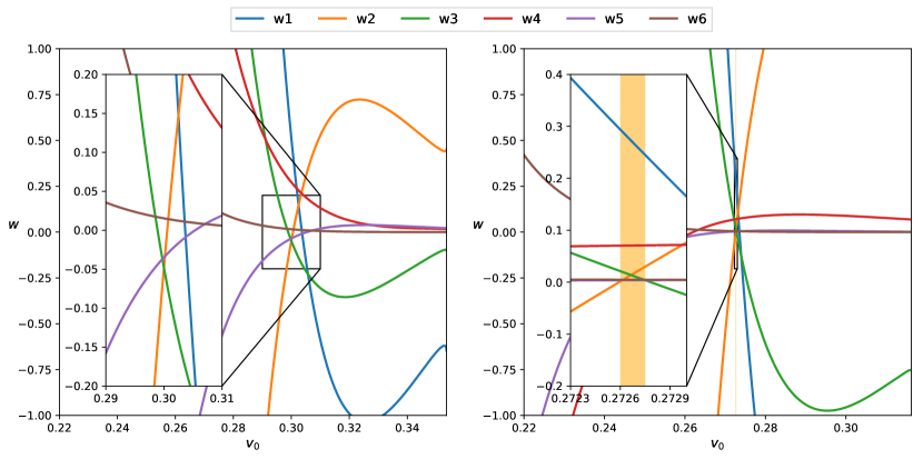
Figure 6: Visual representation of the parametric solution of Eq. 50, having chosen $\tilde{m}=5$. The left panel makes use of the stencil $G=\{(0,0)\bigcup(\pm 1,0)_{\texttt{FS}}\bigcup(\pm 1,\pm 1)_{\texttt{FS}}\bigcup(\pm 2,0)_{\texttt{FS}}\bigcup(\pm 2,\pm 1)_{\texttt{FS}}$ $\bigcup(\pm 2,\pm 2)_{\texttt{FS}}\}$. The panel on the right was obtained using the stencil $G=\{(0,0)\bigcup(\pm 1,0)_{\texttt{FS}}\bigcup(\pm 1,\pm 1)_{\texttt{FS}}\bigcup(\pm 2,\pm 1)_{\texttt{FS}}\bigcup(\pm 2,\pm 2)_{\texttt{FS}}$ $\bigcup(\pm 3,\pm 1)_{\texttt{FS}}\}$. In this second case we can identify a region for which $w_{i}(v_{0})\geq 0~{}\forall i$ (orange colored interval), giving a set of solutions that can be used to build a numerically stable quadrature.

Taking for example $v_{0}=0.2726$, the corresponding weights for the quadrature are:

$$w_{1}=0.2938928682119484\dots~{},\quad w_{2}=0.00136644441345044\dots~{},$$

$$w_{3}=0.0212650236700010\dots~{},\quad w_{4}=0.07032872215612153\dots~{},$$

$$w_{5}=0.0036974948602444\dots~{},\quad w_{6}=0.00477018784553696\dots~{}.$$

Particularly convenient values of $v_{0}$ are those located at the boundaries of the orange colored interval in Fig. 6b, since some weights become zero thus allowing the pruning of certain lattice velocities. In our example one can reduce the full set of $29$ velocities to $25$ by setting either $w_{2}$ to zero (with $v_{0}=0.27259285465\dots$), or $w_{3}$ to zero ($v_{0}=0.27278322823\dots$).

Typically, for a given value of $\tilde{m}$ several different stencils are possible; however, each stencil works correctly only in a certain range of $\tilde{m}$. Still, a reasonably small set of stencils allows to treat $\tilde{m}\geq 0.5$ at the second order and $\tilde{m}\geq 1.2$ at the third order, offering the possibility to cover a very large kinematic regime, from almost ultra-relativistic to non-relativistic.

In general, the process of finding quadratures becomes harder and harder as the order is increased and as $\tilde{m}$ takes smaller and smaller values. The reason is that for $\tilde{m}\rightarrow 0$ the pseudo-particles tend to move all with similar velocities, close to the speed of light, making it difficult to identify a stencil where all particles travel in one time step at different (yet very similar) distances, and still hop from a point of the grid to a neighboring one.

For the limiting case where $\tilde{m}=0$ this translates in restricting to stencils whose elements sit at the intersection between a Cartesian grid and a sphere of given radius. In this case we introduce the parametrization presented in Eq. 53, where following [41] we associate several energy shells to each momentum vector. To give an example, we consider a second order quadrature rule for $\tilde{m}=0$ and solve Eq. 50 by taking the stencil $G=\{(\pm 3,\pm 4)_{\texttt{FS}},(\pm 5,0)_{\texttt{FS}}\}$ (Fig. 5b) and the parametrization in Eq. 53 where three different energy shells get associated to each momentum vector. The solution reads as follows:

$$\tilde{p}_{1}^{0}=0.41577455678\dots ~{}~{}~{}~{}~{}~{}~{}~{}~{}w_{11}=0 w_{21}=0.08888662624\dots$$

$$\tilde{p}_{2}^{0}=2.29428036027\dots ~{}~{}~{}~{}~{}~{}~{}~{}~{}w_{12}=0 w_{22}=0.03481471669\dots$$

$$\tilde{p}_{3}^{0}=6.28994508293\dots ~{}~{}~{}~{}~{}~{}~{}~{}~{}w_{13}=0.00175356541\dots w_{23}=0.00042187435\dots$$

The procedure can be iterated at higher orders, although already at order 4 in 2 spatial dimensions one needs to employ stencils with vectors of length $5\sqrt{13}$, which is impractical from a computational point of view since implies using very large grids to achieve an adequate spatial resolution; things become even more problematic in $(3+1)$ dimensions. Higher orders would most probably require different strategies, e.g. off-lattice schemes, which drastically improve the spatial resolution of the grid, but have as drawbacks the need for interpolation and the introduction of artificial dissipation effects [47, 80, 43]; we do not consider these strategies in this paper.

A special treatment is needed in the $(1+1)$ dimensional case for the massless limit. Indeed, as already remarked in the previous section, in this case the massless limit of both polynomials and projections diverges. It follows that we cannot derive the quadrature through Eq. 50. However, we can exploit the fact that it is still possible to obtain an expression for the expansion of the equilibrium distribution using Eq. 48. We can then express the quadrature problem via the following system of equations:

$$\int f^{\rm eq}((\tilde{p}^{\alpha}),(U^{\alpha}),\tilde{T})\tilde{p}^{\alpha}\dots\tilde{p}^{\omega}\frac{\mathop{}\!\mathrm{d}\tilde{p}^{d}}{\tilde{p}^{0}}=\sum_{i}\sum_{j}w_{ij}f_{N}^{\rm eq}((\tilde{p}_{ij}^{\alpha}),(U^{\alpha}),\tilde{T})\tilde{p}_{ij}^{\alpha}\dots\tilde{p}_{ij}^{\omega},$$ (57)

where we explicitly require the preservation of all the moments of the distribution up to a desired order $N$ and use all the techniques described before to look for the unknown weights $w_{ij}$.

A graphical view of (a subset) of all stencils that we have found at the $2$-nd and $3$-rd order is shown in Appendix H, .

5.4 Forcing Scheme

The definition of force in relativity is subject to a certain degree of arbitrariness due to the lack of certain general properties such as, for example, Newton’s third law. In the following we will use the definition of Minkowski force [58]:

$$K^{\alpha}=\frac{\mathop{}\!\mathrm{d}p^{\alpha}}{\mathop{}\!\mathrm{d}\tau}\quad,$$ (58)

where $\mathop{}\!\mathrm{d}\tau=\frac{1}{\gamma}\mathop{}\!\mathrm{d}t$ is the proper time. From the definition it follows that the spatial components of $(K^{\alpha})$ obey

$$\bm{K}=\gamma~{}\bm{F}\quad,$$ (59)

with $\bm{F}$ the non-relativistic force vector, whereas the time component is such to satisfy

$$K^{\alpha}p_{\alpha}=K^{0}p^{0}-\bm{K}\cdot\bm{p}=0\quad.$$ (60)

Starting from Eq. 39, our task consists in discretizing the term

$$F^{\rm ext}=\frac{mK^{\alpha}}{p^{0}}\frac{\partial f}{\partial p^{\alpha}}\quad.$$ (61)

by taking into consideration the effects of external forces on the (pseudo)-particles used in our description.

Following [81], we assume the distribution function to be not far from equilibrium,

$$\frac{\partial f}{\partial p^{\alpha}}\approx\frac{\partial f^{\rm eq}}{\partial p^{\alpha}}\quad;$$ (62)

at this point, we use the polynomial expansion of the equilibrium distribution

$$\frac{\partial f}{\partial p^{\alpha}}\approx\frac{\partial f^{\rm eq}}{\partial p^{\alpha}}=\omega(p^{0})\sum_{k=0}^{\infty}b^{(k)}((U^{\mu}),T)J^{(k)}((p^{\mu}))\quad,$$ (63)

with the projection coefficients defined as

$$b^{(k)}((U^{\mu}),T)=\int\frac{\partial f^{\rm eq}((p^{\mu}),(U^{\mu}),T)}{\partial p^{\alpha}}J^{(k)}((p^{\mu}))\frac{\mathop{}\!\mathrm{d}^{d}p}{p^{0}}\quad;$$ (64)

an even simpler approach starts from the observation that the derivative of the analytic Maxwell-Jüttner distribution is given by

$$\frac{\partial f^{\rm eq}}{\partial p^{\alpha}}=-\frac{U_{\alpha}}{T}f^{\rm eq}\quad,$$ (65)

leading to

$$F^{\rm ext}\approx-\frac{m}{T}\frac{K^{\alpha}U_{\alpha}}{p_{0}}f^{\rm eq}\quad,$$ (66)

which has the clear advantage of requiring one single evaluation of the equilibrium distribution. Both approaches yield consistent results, as we show later on.

As a general remark, the use of the polynomial expansion of the equilibrium distribution is not particularly useful in the relativistic case as it is non trivial to identify the relationship between the coefficients $a^{(k)}$ and $b^{(k)}$ leading to cumbersome analytical form of the resulting expressions and significant computational overheads in the evaluation of the external force; this is even more so, as in our case it is not possible – as customary in non relativistic LB methods – to translate the effect of an external force into a shift in the macroscopic variables of interest [82, 83, 84, 85].

6 Numerical recipes

In this section we provide details on how to implement a RLBM simulation. We discuss the conversion from physics to lattice units, the numerical scheme and a few practical aspects related to implementations on modern parallel architectures.

6.1 From Physical to Lattice units

To relate physical space and time units with the corresponding lattice units, it is convenient to start by assigning the physical length $\delta x$, corresponding to one lattice spacing. Suppose we use $N$ grid points to represent the physical length $L$, the corresponding lattice spacing $\delta x$ is then:

$$\delta x=\frac{L}{N}\quad.$$ (67)

Time and space units are implicitly linked via Eq. 43, where at each time step pseudo-particles move from position $\bm{x}$ to $\bm{x}+\bm{v}^{i}\delta t$. Since we constrain both source and destination positions to lie on a Cartesian grid, it follows:

$$v_{0}N_{i}\delta t=N_{i}\delta x\quad,$$ (68)

with $N_{i}\in\mathbb{Z}^{d}$. This, in turn, provides the following relation between time and space units in the lattice:

$$v_{0}=\frac{\delta x}{\delta t}\quad,\frac{v_{0}}{c}=\frac{\delta x}{c\delta t}$$ (69)

The conversion of all mass and energy related quantities is performed by choosing a value for the reference temperature $T_{0}$ and a corresponding value for the reference energy $k_{B}T_{0}$, already encountered in the previous sections in the definition of non-dimensional quantities on the lattice. While the choice of $T_{0}$ is in principle arbitrary, a sensible choice can have a major impact on the accuracy of the results. In fact one can expect better results when $T_{0}$ is chosen such that the numerical values of the temperature in lattice units are $\sim 1$, since such value was used as expansion origin for the equilibrium distribution function.

At this point we have defined the translation of lengths, time and mass units between physics and lattice. The conversion of other derived quantities follows straight. In the following, we provide a few examples, where we distinguish between physics and lattice units, indicating quantities with a $p$ or $l$ subscript respectively. The conversion of the particle number density writes as

$$n_{p}=n_{l}\frac{1}{(\delta x)^{d}}\quad.$$ (70)

Similarly, a generic velocity can be converted using

$$v_{p}=v_{l}\frac{\delta x}{\delta t}=v_{l}~{}v_{0}\quad.$$ (71)

As a final example we translate in lattice units the shear viscosity, for which we take the general expression

$$\eta_{p}=f(\zeta)P_{p}\tau_{p}\quad,$$ (72)

with $f(\zeta)$ a function solely depending on the dimensionless relativistic parameter $\zeta$. Using the EOS of an ideal gas we can write:

$$\eta_{p}=f(\zeta)n_{p}k_{B}T_{p}\tau_{p}=f(\zeta)\frac{n_{l}}{(\delta x)^{d}}T_{l}k_{B}T_{0}\tau_{L}\delta t=\eta_{L}k_{B}T_{0}\frac{\delta t}{(\delta x)^{d}}\quad.$$ (73)

6.2 Relativistic Lattice Boltzmann Algorithms

The initial conditions for the RLBM algorithm consist in prescribing the values of $f_{i}(\bm{x},t_{0})$ at the initial time $t_{0}$. A typical choice is to prescribe the equilibrium distribution function with a given initial profile for temperature, density and velocity, thus setting $f_{i}(\bm{x},t_{0})=f_{i}^{\rm eq}$.

For each time step, the following operations are performed to evolve the distribution function at each single grid point:

1. We start by computing the first and second moment of the distribution:

   $$N^{\alpha}=\sum_{i}f_{i}\tilde{p}^{\alpha}_{i}\quad,$$

   $$T^{\alpha\beta}=\sum_{i}f_{i}\tilde{p}^{\alpha}_{i}\tilde{p}^{\beta}_{i}\quad.$$

2. The energy density $\epsilon$ and the four velocity $U^{\alpha}$ are obtained solving the eigenvalue problem:

   $$\epsilon U^{\alpha}=T^{\alpha\beta}U_{\beta}\quad,$$

   with $\epsilon$ corresponding to the largest eigenvalue of $T^{\alpha\beta}$, and $U^{\alpha}$ being the correspondent eigenvector.

3. Next, we compute the particle density from

   $$n=U_{\alpha}N^{\alpha}\quad.$$

4. We then compute the temperature from the EOS (see Section 3).

5. We now have all the fields required to compute the equilibrium distribution function:

   $$f_{iN}^{\rm eq}((\tilde{p}^{\mu}),(U^{\mu}),\tilde{T})=w_{i}\sum_{k=0}^{N}a^{(k)}((U^{\mu}),\tilde{T})J^{(k)}((\tilde{p}_{i}^{\mu}))\quad.$$

6. If present, we compute the Minkowski forcing term (see Section 5.4).

7. We determine the local value of the relaxation time $\tau$ (which typically is either a constant or determined in such a way that the ratio of shear viscosity and entropy density $\eta/s$ is constant).

8. Finally, we evolve the system over one time step, via the discrete Boltzmann equation:

   $$f_{i}(\bm{x}+\bm{v}^{i}\Delta t,t+\Delta t)=\left(1-\Omega\right)f_{i}(\bm{x},t)+\Omega f_{i}^{\rm eq}(\bm{x},t)+F_{i}^{\rm ext}$$

   where

   $$\Omega=\Delta t~{}\frac{\tilde{p}_{i}^{\mu}U_{\mu}}{\tilde{p}^{0}\tau}\quad.$$

   is the dimensionless relaxation parameter controlling the transport coefficients.

6.3 Parallel implementation on GPUs.

One of the main reasons for the widespread resort to LBM algorithms is computational efficiency [86]. The strength of LBM is embedded in the stream-collide paradigm, which, being numerically -exact- (zero roundoff), stands in contrast with the advection-diffusion scheme used in a macroscopic fluid-flow representation.

The streaming phase consists in moving particles according to the discrete velocities defined by the stencil, and thus, unlike advection, following a regular pattern regardless of the complexity of the fluid flow. Moreover, streaming is exact in the sense that there is no round-off error since it consists only of memory shifts, with no floating-point operations involved. We remark that efficient memory access has become a main point of optimization in the modern large-scale implementations [87, 88, 89, 86].

Instead, the collide step performs all the floating-point operations required to implement the collisional operator. The locality of the collisional operator makes it possible to update each grid point in parallel, making LBM an excellent target for highly scalable implementations on modern HPC architectures.

The relativistic formulation presented in the previous sections preserves all the computational virtues of the classical algorithm. The complexities in the analytic expressions of the polynomial expansion of the distribution, in the EOS (etc..), reflects in a significantly higher demand of floating point operations required to update a single grid point, easily one or two orders of magnitude more with respect to the classical LBM.

In Tab 1, we collect a few figures of merit regarding the performances of RLBM codes in 2 and 3 dimensions on a recent NVIDIA Pascal GPU. The simulation parameters are the same used in the Green-Taylor vortex benchmark described in Section 7.1. We simulate the specific case $\zeta=5$ on a periodic square grid of $512^{2}$ points in 2d, and $192^{3}$ points in 3d, using the following stencils: $G=\{(0,0)$ $\bigcup(\pm 1,0)_{\texttt{FS}}$ $\bigcup(\pm 1,\pm 1)_{\texttt{FS}}$ $\bigcup(\pm 2,0)_{\texttt{FS}}$, $\bigcup(\pm 2,\pm 1)_{\texttt{FS}}$ $\bigcup(\pm 2,\pm 2)_{\texttt{FS}}$ $\bigcup(\pm 3,0)_{\texttt{FS}}$, $\bigcup(\pm 3,\pm 2)_{\texttt{FS}}$ $\bigcup(\pm 3,\pm 3)_{\texttt{FS}}$ $\bigcup(\pm 4,0)_{\texttt{FS}}$ $\}$, for the 2d case, and $G=\{(0,0,0)$ $\bigcup(\pm 1,0,0)_{\texttt{FS}}$ $\bigcup(\pm 1,\pm 1,\pm 1)_{\texttt{FS}}$ $\bigcup(\pm 2,0,0)_{\texttt{FS}}$ $\bigcup(\pm 2,\pm 1,\pm 1)_{\texttt{FS}}$ $\bigcup(\pm 2,\pm 2,0)_{\texttt{FS}}$ $\bigcup(\pm 2,\pm 2,\pm 1)_{\texttt{FS}}$ $\bigcup(\pm 2,\pm 2,\pm 2)_{\texttt{FS}}$ $\bigcup(\pm 3,0,0)_{\texttt{FS}}$ $\bigcup(\pm 3,\pm 1,\pm 1)_{\texttt{FS}}$ $\bigcup(\pm 3,\pm 2,0)_{\texttt{FS}}$ $\}$ for the 3d case, where we recall FS stands for full-symmetric.

Thanks to the high arithmetic intensity of the algorithm (defined as the ratio of total floating-point operations to total data movement), it is comparatively simple to sustain a large fraction of the performance peak of the target architecture. A detailed analysis on the GPU-porting and optimization of RLBM will be reported elsewhere.

	2D RLBM ($\zeta=5$)	3D RLBM ($\zeta=5$)
Stencil vectors	45	143
FLOP/site	$\sim 66000$	$\sim 210000$
Arithmetic intensity	92	92
Collide MLUPS	55	14
Collide TFLOPS (${\cal E}_{c}$ %)	3.7 (70 %)	3.1 (60 %)

Table 1: Overview of the performances of a NVIDIA Pascal P100 GPU (1792 cores for a performance peak of 5.3 TFLOPS in double precision arithmetics) running our RLBM codes in 2 and 3 space dimensions. We list the number of floating point operations (FLOP) required to update one grid point, the arithmetic intensity and the performance of the collide kernel, expressed both in MLUPS (Million Lattice Updates per Second) and TFLOP per second. ${\cal E}_{c}$ is an estimate of the GPU sustained performance with respect to peak performance.

7 Numerical Results I: Calibration of Transport Coefficients

In section 4 we have summarized the steps needed to derive the analytical expressions for the transport coefficients of an ideal relativistic gas in $(d+1)$ dimensions, using both Chapman-Enskog and Grad’s moments method. Unfortunately, to the best of our knowledge, no experimental setup is available to discern which (if any) of the two methods gives the correct results. For this reason, the lattice kinetic scheme developed in the previous pages can be used to tell the two methods apart.

Here we summarize and extend the results presented in [45, 47, 49, 90], which show that the transport coefficients calculated following Chapman-Enskog’s approach are in better agreement with numerical results than those obtained via using Grad’s method. We present numerical results for the shear viscosity, thermal conductivity and of the bulk viscosity as well. In addition, we extend previous results to $1,2,3$ space dimensions.

The numerical results presented in this section base on schemes using third order quadratures, which are made available as supplemental information [76].

7.1 Shear viscosity

As discussed in Section 4, the analytic form for the shear viscosity predicted by the Chapman-Enskog expansion and Grad’s method of moments is different. Both methods provide results in the form

$$\eta=f(\zeta)P\tau\quad,$$ (74)

but with a different dependence on the relativistic parameter $\zeta$, as expressed in the above equation by the function $f(\zeta)$ (see Appendix C for the analytic expression of $f(\zeta)$ in the two cases and for a full comparison).

Here, we describe the procedure followed to measure $f(\zeta)$ from simulations. We first consider an almost divergence-free flow, which allows to neglect compressible effects, and to simplify the energy-momentum tensor to

$$T^{\alpha\beta}=(\epsilon+P)U^{\alpha}U^{\beta}-P\eta^{\alpha\beta}+\pi^{<\alpha\beta>}\quad.$$ (75)

As a benchmark, we take the Taylor-Green vortex [91], a well known example of a decaying flow, exhibiting an exact solution for the classical Navier-Stokes equations, and for which we can derive an approximate solution in the relativistic regime. We start from the following initial conditions, in a $d>1$ periodic domain,

$$u_{x} =\phantom{-}u_{0}\cos(x)\sin(y)\quad x,y\in[0,2\pi]\quad,$$ (76)

$$u_{y} =-u_{0}\cos(y)\sin(x)\quad,$$

$$u_{z} =u_{w}=\dots=0\quad.$$

with $u_{0}$ a given value for the initial velocity, and assume that the time dependent solution takes the same form as in the classical case:

$$u_{x} =\phantom{-}u_{0}\cos(x)\sin(y)F(t)\quad x,y\in\left[0,2\pi\right]\quad,$$ (77)

$$u_{y} =-u_{0}\cos(y)\sin(x)F(t)\quad,$$

$$u_{z} =u_{w}=\dots=0\quad.$$

In order to determine the analytic expression of $F(t)$, we solve the conservation equations by inserting, starting from Eq. 75:

$$\partial_{\beta}T^{\alpha\beta}=(\epsilon+P)U^{\alpha}\partial_{\beta}U^{\alpha}+\partial_{\beta}\pi^{<\alpha\beta>}=0$$ (78)

Next, we plug Eq. 77 into Eq. 78 and perform a first order expansion of the resulting expression, giving

$$\begin{bmatrix}0\\ \phantom{-}U^{0}(\epsilon+P)\sin{(x)}\cos{(y)}F^{\prime}(t)\\ -U^{0}(\epsilon+P)\cos{(x)}\sin{(y)}F^{\prime}(t)\\ 0\end{bmatrix}+\begin{bmatrix}0\\ \phantom{-}2\eta U^{0}F(t)\sin{(x)}\cos{(y)}\\ -2\eta U^{0}F(t)\cos{(x)}\sin{(y)}\\ 0\end{bmatrix}=\begin{bmatrix}0\\ 0\\ 0\\ 0\end{bmatrix}$$ (79)

where for improved readability we have kept separated the two additive terms of Eq. 78.

From the above we directly get the following differential equation:

$$2\eta F(t)+(P+\epsilon)F^{{}^{\prime}}(t)=0\quad,$$ (80)

which can be solved under the assumption of an (approximately) constant value of $P+\epsilon$:

$$F(t)=\exp{\left(-\frac{2\eta}{P+\epsilon}t\right)}F(0)\quad.$$ (81)

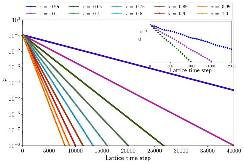
Figure 7: Simulated time evolution of $\bar{u}$ for selected $\tau$ values on a $L=400$ square lattice. Simulation are performed using a $(3+1)$-dimensional solver, with initial numerical parameters $\zeta=0$, $u_{0}=0.2$, $n=1$, $T=1$. Dashed lines are fits to the exponential decay predicted by Eq. 81. The inset shows non-linear effects in the early phases of the flow.

Next, it is expedient to introduce an observable $\bar{u}(t)$,

$$\bar{u}^{2}(t)=\int_{0}^{2\pi}\int_{0}^{2\pi}\left(u_{x}^{2}(t,x,y)+u_{y}^{2}(t,x,y)\right)\mathop{}\!\mathrm{d}x\mathop{}\!\mathrm{d}y\quad,$$ (82)

that is directly proportional to $F(t)$, as easily seen from Eqs 77. We perform several simulations of the Taylor-Green vortex, on periodic boxes of side $L=400$. Temperature and density are set to unity on each grid point, while the velocity fields is initialized using Eq. 76 and with $u_{0}=0.2$. In order to better characterise the numerical fit of $f(\zeta)$, we consider a broad range of $\zeta$ values, smoothly bridging between ultra-relativistic to near non-relativistic regimes. The relaxation of time is set to a constant value throughout each simulation, with numerical values spanning between $0.6$ and $1.0$; at fixed time intervals we then get an estimate for $\bar{u}^{2}(t)$, calculated as:

$$\bar{u}^{2}(t)=\frac{1}{L^{2}}\sum_{i=1}^{L}\sum_{j=1}^{L}u_{x}(t,i,j)^{2}+u_{y}(t,i,j)^{2}\quad.$$ (83)

In Fig. 7, we show a few example of simulations, featuring the time evolution of $\bar{u}$, with $\zeta=0$ and for several different values of the relaxation time, clearly exhibiting an exponential decay.

For each set of mesoscopic values, we perform a linear fit of $\log(\bar{u})$ extracting a corresponding value of $\eta$ via Eq. 81. Finally, by comparison with Eq. 74, we estimate the value of $f(\zeta)$ at different values of $\zeta$. In Table 2, we show a few results obtained following this procedure in the $(3+1)$-dimensional case. One appreciates that, for each different value of $\zeta$, measurements of $\eta(\tau)$ yield a constant value of $f(\zeta)$.

	$f(\zeta)$
$\tau$	$\zeta$ = 0	$\zeta$ = 1.6	$\zeta$ = 2	$\zeta$ = 3	$\zeta$ = 4	$\zeta$ = 5	$\zeta$ = 10
0.600	0.8003	0.8319	0.8448	0.8587	0.8892	0.8994	0.9311
0.700	0.8002	0.8318	0.8447	0.8584	0.8888	0.8990	0.9302
0.800	0.8002	0.8318	0.8447	0.8583	0.8887	0.8989	0.9300
0.900	0.8002	0.8318	0.8447	0.8583	0.8887	0.8988	0.9299
1.000	0.8002	0.8317	0.8446	0.8582	0.8887	0.8988	0.9299

Table 2: Selected sample values for the estimate of the parameter $f(\zeta)$ for several values of $\tau$ and $\zeta$. Statistical errors for all entries are smaller than $1$ in the last displayed digit.

Moreover, from the second column of Tab. 2, we obtain $f(0)=4/5$ to very high accuracy, which is consistent with the result of the Chapman-Enskog expansion in the ultra-relativistic limit (see Eq. 31). In Fig. 8, we show that the CE prediction almost perfectly matches the results of the simulations (and we remark that no free parameters are involved in this comparison) over a broad range of values of $\zeta$, in both $(2+1)$ and $(3+1)$-dimensions. For the $(1+1)$-dimensional case, we only show the analytic results since in this case we do not have a suitable benchmark with an approximate analytic solution that can be used to numerically fit the curve.

To conclude, in the inset in Fig. 8 we show two effects: i) the impact of the grid resolution on the quality of the estimate ii) the way different quadratures provide slightly different results. In the example shown we have focused in the case $d=2$, $\zeta=2$. We perform simulations using two different quadratures, with the green dots obtained using the stencil $QA=\{(0,0)$, $(\pm 1,\pm 1)_{\texttt{FS}}$, $(\pm 2,\pm 2)_{\texttt{FS}}$, $(\pm 3,\pm 4)_{\texttt{FS}}$, $(\pm 5,0)_{\texttt{FS}}$, $(\pm 5,\pm 5)_{\texttt{FS}}$, $(\pm 6,\pm 2)_{\texttt{FS}}$, $(\pm 6,\pm 3)_{\texttt{FS}}$, $(\pm 6,\pm 4)_{\texttt{FS}}$, $(\pm 7,\pm 1)_{\texttt{FS}}$ $\}$, while the black ones base on the stencil $QB=\{(0,0)$, $(\pm 1,\pm 2)_{\texttt{FS}}$, $(\pm 3,\pm 4)_{\texttt{FS}}$, $(\pm 4,\pm 4)_{\texttt{FS}}$, $(\pm 5,\pm 5)_{\texttt{FS}}$, $(\pm 6,0)_{\texttt{FS}}$, $(\pm 6,\pm 3)_{\texttt{FS}}$, $(\pm 6,\pm 4)_{\texttt{FS}}$, $(\pm 7,\pm 1)_{\texttt{FS}}$, $(\pm 7,\pm 2)_{\texttt{FS}}$ $\}$. For each quadrature we perform a convergence test with respect to the grid size, showing that the estimates tend to stabilize to a constant values as soon as $L\geq 200$. We attribute the differences observed in the results provided by the two quadratures in the different error committed in the approximation of the higher order tensors; note that the corresponding results differ from each other by approximately 1-2%, which we can consider an estimate of our systematic error.

Figure 8: Comparison of the non-dimensional shear viscosity for a relativistic gas in (1+1), (2+1) and (3+1) dimensions, obtained using Chapman-Enskog and Grad’s methods. Dots represent numerical measurements of the shear viscosity simulating the time decay of Taylor-Green vortex using RLBM. The inset shows a grid-convergence test for the estimated value of the shear in viscosity in the bidimensional case at $\zeta=2$; black and green dots represent the estimates obtained using two different third order quadratures (see the main text for their definition), showing small discrepancies of about $2\%$.

7.2 Thermal conductivity

The numerical measurements of the thermal conductivity follow the same general steps described in detail in the previous section. We consider a numerical setup for simulating two parallel plates, kept at different constant temperatures $T_{\rm hi}$ and $T_{\rm lo}$, with $\Delta T=T_{\rm hi}-T_{\rm lo}$. For sufficiently small values of $\Delta T$, the flow can be approximated to be non-relativistic and as a consequence Eq. 25 reduces to Fourier’s law:

$$q^{\alpha}=\lambda\nabla^{\alpha}T\quad.$$ (84)

Under these settings, simulations reach a steady state with an approximately constant temperature gradient, and a constant heat flux $q^{\alpha}$ which can be calculated in simulations using Eq. 22:

$$q^{\alpha}=h_{e}(N_{E}^{\alpha}-N^{\alpha})\quad.$$ (85)

Combining the two equations above, it is possible to estimate the thermal conductivity $\lambda$ and discern between the expressions predicted respectively by Chapman-Enskog and Grad’s methods (once again, refer to Appendix C for the d-dimensional analytical form of $\lambda$ for the two cases).

Similarly to the case of shear viscosity $\eta$, we perform several simulations varying the mesoscopic parameters $\tau$ and $\zeta$. The simulations are performed on a rod represented using $1600$ points along the $x$ axis, with all the other dimensions represented by $1$ single point, with periodic boundary conditions. The leftmost and rightmost points are kept stationary by imposing the equilibrium distribution calculated with a temperature in numerical units of respectively $T_{\rm hi}=1.005$ and $T_{\rm lo}=0.995$, zero velocity, while the density is obtained by linear interpolation from the neighboring interior points. In order to calculate an estimate for the thermal conductivity the system is evolved until a steady state is reached. From the final configuration we then compute an approximation of the temperature gradient using central finite difference. Next, we compute spatial averages of the quantities $<\nabla^{\alpha}T>_{x}$ and $<q^{x}>_{x}$ which we use in combination with Eq. 84 to get an estimate for $\lambda$.

The results obtained are summarized in the plots in Fig. 9, showing that in 1, 2 and 3 spatial dimensions, the numerics are in excellent agreement with the predictions of the Chapman-Enskog expansion.

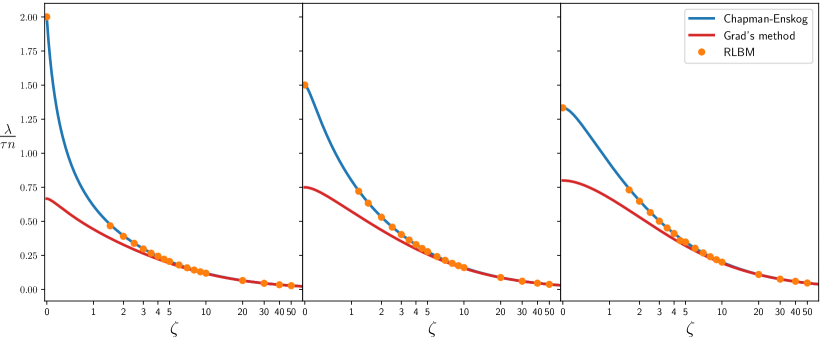
Figure 9: Comparison of the non-dimensional thermal conductivity for a relativistic gas in (1+1), (2+1) and (3+1) dimensions, obtained using Chapman-Enskog and Grad’s methods. Dots represent numerical measurements from RLBM simulations.

7.3 Bulk viscosity

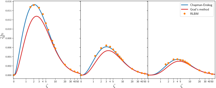
Figure 10: Comparison of the non-dimensional bulk viscosity for a relativistic gas in (1+1), (2+1) and (3+1) dimensions, obtained using Chapman-Enskog and Grad’s methods. Dots represent numerical measurements from RLBM simulations.

The measurement of the bulk viscosity requires the analysis of a flow with sizable compressibility effects. A popular example that serves our purpose is the Riemann problem and the generation of shock waves (which will be studied in detail in the forthcoming sections). However, the presence of strong discontinuities makes the numerical analysis challenging and the error committed in our data-fits too large to discriminate between the predictions of the analytic form of the bulk viscosity $\mu$ due to Chapman-Enskog and Grad’s method. We therefore turn to the analysis of a time decaying sinusoidal wave, which still gives the possibility to observe compressible effects, yet with the advantage of well behaved derivatives.

We consider a periodic domain with the following initial condition:

$$u_{x} =u_{0}\sin(x)\quad x\in[0,2\pi]\quad,$$ (86)

$$u_{y} =u_{z}=\dots=0\quad.$$

with $u_{0}$ a given initial velocity. Particle density and temperature are initially set to a constant value. In the simulations we measure the dynamic pressure $\varpi$ from the trace of the energy momentum tensor (Eq. 23):

$$\varpi=-\frac{1}{d}(T^{\mu}_{\mu}-{T_{E}}_{\mu}^{\mu})\quad.$$ (87)

By combining the above equation with Eq. 27 it is then possible to perform numerical measurements of the bulk viscosity through

$$\mu=-\frac{\varpi}{\nabla_{\alpha}U^{\alpha}}\quad.$$ (88)

We perform simulations on a mono-dimensional system with $1600$ used to represent the $x$ axis, and $1$ single point for all the other components and periodic boundary conditions. Density and temperature are set to unit, while the initial amplitude of the wave is set to $u_{0}=10^{-5}$. Like in the previous cases discussed in this section, we perform several simulations with different values of the mesoscopic parameters $\tau$ and $\zeta$, and perform the following steps to obtain accurate measures of the bulk viscosity: i) we follow the time evolution of the system for half a period of the sine wave and at each time step $t$ we compute $\varpi$ via Eq. 87 and calculate an estimate of $\nabla_{\alpha}U^{\alpha}$ using a central finite difference scheme. ii) we calculate the spatial average $<\mu(t)>_{x}$ from Eq. 88, ignoring points where $|\nabla_{\alpha}U^{\alpha}|<10^{-10}$. iii) we improve our estimate for $\mu$ by averaging on several time steps.

The results results presented in Fig. 10 lead to the same conclusions as for $\eta$ and $\lambda$, with clear evidence that the Chapman-Enskog procedure is in excellent agreement with the numerical results.

We conclude this section with a remark: As shown in Fig 8- 10 our simulations do not cover the domain $0<\zeta\lesssim 1$. The reason, as it has been explained in Section 5.3, is that in this parameter range the definition of quadratures lying on Cartesian grid becomes a hard task since the physical constrains that one needs to satisfy are not suitable for a lattice formulation. While off-lattice quadratures would allow the description of wider a kinematic range, the numerical evaluation of the transport coefficients would have been weakened by the numerical artifacts introduced by an interpolation scheme.

8 Numerical Results II: Benchmark and Validation

In this section we provide a few validation tests together with example of applications of the RLBM. We start with the validation of the forcing scheme which we use to reproduce the results of a simple non-relativistic Poiseuille-flow. We then consider the Riemann problem, a benchmark commonly used in both non-relativistic and relativistic numerical hydrodynamics, in order to assess the stability and the accuracy of numerical solvers. We validate the code in a nearly inviscid regime, for which analytic solutions are available, then explore viscous regimes for fluid of both mass-less and massive particles, comparing with other numerical solvers available in the literature.

Next, we give an example of simulation in three spatial dimensions, relevant for the study of the early stage formation of the quark-gluon plasma.

We conclude by presenting simulations of the electrons flow in graphene, studying realistic setups which have been recently used in actual experiments.

8.1 Validation of the forcing scheme

In Section 5.4 we have presented two approaches to introduce a generic Minkowski force $K^{\alpha}$ in the numerical scheme. Benchmark that can be adopted for testing the correctess of the forcing scheme are not abundant: among them we list Ref. [92], in which a computation of electric conductivity in a QGP [92] is performed. Here we follow an even simpler approach and take into consideration the effect of applying a weak gravitational field to the (pseudo)-particles forming a relativistic fluid. In the non-relativistic case, the most standard benchmark is given by the Poiseuille-flow, describing the motion of a fluid between two parallel plates under the effect of gravity (or of a pressure gradient).

In the following, we will then directly compare with the analytic solution of the classical Poiseuille-flow, assuming a sufficiently small gravity acceleration $\bm{g}$. Starting from Eq. 59, we can define the Minkowski force in terms of $\bm{g}$ as

$$\bm{K}=\gamma~{}\bm{F}=\gamma~{}m\bm{g}=\frac{p^{0}}{c}\bm{g}\quad.$$ (89)

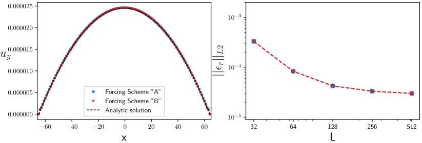
Figure 11: Validation of the forcing scheme for the RLBM algorithm by solving a non-relativistic Poiseuille flow. In the left panel we show the parabolic velocity profile obtained using a RLBM scheme in two spatial dimensions, working on a $L\times 64$ grid, and considering two different implementations of the forcing scheme: In scheme ”A” the forcing term is discretized using a polynomial expansion, while for scheme ”B” we compute explicitly the derivative of the Maxwell-Jüttner distribution (see Section 5.4 for details). The panel on the right shows the relative error, computed with respect to the analytic solution. Both solution provide the same level of accuracy, with the error decreasing as the grid size is increased.

In Fig. 11 we validate the two different implementations of the forcing scheme described in section 5.4: We call scheme ”A” the forcing term discretized using a polynomial expansion, while scheme ”B” refers to the case where we compute explicitly the derivative of the Maxwell-Jüttner distribution. We work in two spatial dimensions and perform simulations on grids of size $L\times 64$. Periodic boundary conditions are applied along the $y$-axis, while at $x=0$ and $x=L-1$ no-slip boundary conditions are used to simulate two parallel plates. We apply a gravity-like force acting parallel to the wall boundaries, of magnitude $|\bm{g}|=10^{-8}$ in numerical units.

In the left panel in Fig. 11 we can see that both implementations of the forcing term correctly reproduce the parabolic profile of the fluid flow. On the right panel we also show a more quantitative comparison, with the relative error as a function of the number of points $L$ used to represent the box width. The right panel in Fig. 11 shows the relative error computed with respect to the analytic solution as:

$$\epsilon_{r}=\sqrt{\frac{\sum_{x}\left(u_{y}(x)-u^{\rm ref}_{y}(x)\right)^{2}}{\sum_{x}\left(u^{\rm ref}_{y}(x)\right)^{2}}}\quad,$$ (90)

where we consider the analytic solution of the classic Poiseuille flow:

$$u^{\rm ref}_{y}(x)=\frac{|\bm{g}|}{2\nu}x(x-L)\quad.$$ (91)

The relative error shows saturation at a plateau value of about $10^{-5}$. This is due to the specific procedure adopted to apply the non-slip boundary conditions at the solid walls, which consists of imposing a local equilibrium at zero flow speed. This provides a dramatic gain in simplicity at the cost of ignoring non-equilibrium effects due to the near-wall velocity gradient. The standard bounce-back technique, ensuring second order accuracy is conceptually straightforward but extremely laborious in the presence of solid boundaries, due to the large number of discrete velocities implied. For the purpose of the present benchmark, we have opted for simplicity, also on account of the fact that, consistently with previous work [93], for slow flows such as those of Fig. 11, the relative error appears to be quite negligible. Should the physical problem require the handling of fast flows with strong near-wall gradients, a more accurate treatment of boundary conditions would certainly be needed.

While the differences between scheme ”A” and ”B” are negligible in terms of precision, they are instead relevant in terms of computational requirements. Comparing the execution time for the simulations used to produce the results in Fig. 11 we observe that scheme ”A” is $1.5-1.7$ times more expensive than ”B”, due to the necessity to compute the extra terms in the polynomial expansion of the force term. These overheads can be even larger in 3-dimensions, where the coefficients of the expansions depend on Bessel functions.

8.2 Relativistic Sod’s Shock tube

The 1-d Riemann shock tube test is a widely adopted benchmark for the validation of numerical hydrodynamics methods. This benchmark has an exact time-dependent solution, both in the non-relativistic [94] and in the relativistic [95, 9] regimes, and can be used to test the ability of a numerical solver to evolve flows in the presence of strong discontinuities and large gradients.

From a physical point of view, the problem consists of a tube filled with a gas which initially is in two different thermodynamical states on either side of a membrane placed at $x=0$. As a result, the macroscopic quantities describing the fluid present a discontinuity at the membrane. Once the membrane is removed the discontinuities decay producing shock/rarefaction waves, depending on the initial configuration chosen for the two different chambers.

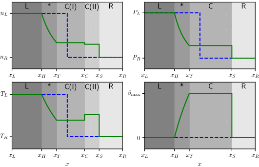
Figure 12: Example of analytic solution of the Sod’s shock tube problem in the inviscid limit, for an ultra-relativistic equation of state in $(3+1)$ dimensions. Region $L$ and $R$ have not been reached yet by the rarefaction wave and preserve therefore their initial state; region $*$ contains the rarefaction wave. The shock wave is present in regions $C(I)$ and $C(II)$ and the interface between these regions is associated to discontinuities in density and temperature. The blue dotted lines represent the initial conditions while the green lines represent the solution at a certain time $t>0$.

The Sod’s shock tube problem is a particular instance of the Riemann problem, with the following initial conditions:

$$(P,n,\beta)=\begin{cases}(P_{\rm L},n_{\rm L},0)&x<0\\ (P_{\rm R},n_{\rm R},0)&x>0\end{cases}\quad.$$ (92)

Let us assume $n_{\rm L}>n_{\rm R}$ and $P_{\rm L}>P_{\rm R}$, where the subscript $\rm L$ and $\rm R$ refer respectively to the left and right sides of the membrane. With these initial conditions, the time evolution of the flow is characterized by two distinct components: a rarefaction wave traveling from the initial field discontinuity to the left, and a shock wave traveling from the initial field discontinuity to the right.

If we consider an inviscid fluid, it is possible to describe the time evolution of the system analytically by solving the conservation equations. However, the derivation of a solution in regimes other than the classical and ultra-relativistic one is a hard task which necessarily requires numerical integrations [95]. For this reason we restrict the first part of our analysis to the ultra-relativistic regime.

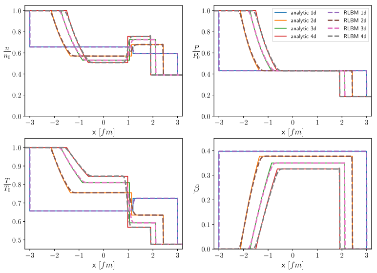
Figure 13: Sod’s shock tube for a gas of massless particles in (d+1)-dimensions (d=1,2,3,4), at $t=3.0~{}\rm{fm/c}$. Lines represent the analytic solution, while dotted lines are result of RLBM simulations at $\eta/s=0.002$. Top: left) temperature profile right) pressure profile. Bottom: left) density profile right) $\beta=|U^{i}|/U^{0}$. All macroscopic quantities are plotted in non-dimensional units by dividing for their correspondent initial values at $x=-3.0~{}\rm{fm}$. All numerical results are obtained using third order quadratures (see Appendix H.2 for details on the velocity sets), using $6400\times 1\times 1$ grids.

At a given time $t>0$, the flow domain can be characterized by defining the different macroscopic quantities in the five regions shown in Fig. 12. Their definition, together with the general d-dimensional analytical solution, is reported in Appendix D.

For testing the inviscid regime we consider the following initial setup: $P_{\rm L}=5.43~{}\rm{GeV/fm^{3}}$ and $P_{\rm R}=1~{}\rm{GeV/fm^{3}}$, with corresponding initial temperatures $T_{\rm L}=400~{}\rm{MeV}$ and $T_{\rm R}=190~{}\rm{MeV}$. In order to convert from physics to lattice units we follow the discussion in section 6.1. We start by setting our reference temperature $T_{0}$ equal to $T_{\rm L}$, thus $T_{0}=T_{\rm L}=400~{}\rm{MeV}$, which translates the initial temperatures on the lattice to $T_{\rm L}=1$ and $T_{\rm R}=0.475$. We also choose the initial values for the particle number density to be $n_{\rm L}=1$ and $n_{\rm R}=0.39$, which correctly reproduce the ratio $P_{\rm L}/P_{\rm R}$.

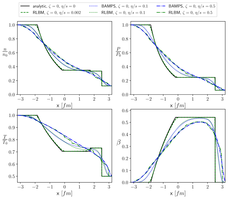
Figure 14: Sod’s shock tube for a gas of massless particles at $t=3.2~{}\rm{fm/c}$, for several values of $\eta/s$. The results of simulations of the RLBM (green lines) at $\eta/s=0.1$ and $\eta/s=0.5$ are compared against the results provided by BAMPS (blue lines). Top: left) density profile right) pressure profile. Bottom: left) temperature profile right) $\beta=|U^{i}|/U^{0}$. Density, temperature and pressure are plotted in non-dimensional units by dividing for their correspondent initial values at $x=-3.2~{}\rm{fm}$. The simulations have been performed on grids of size $6400\times 1\times 1$, using the ultra-relativistic third order quadrature in Appendix H.2.

We perform our tests on a grid of size $L_{x}\times 1\times 1$, half of which represents the physical domain defined in the interval $(-3.2~{}\rm{fm},3.2~{}\rm{fm})$, while the other half forms a mirror image that allows using periodic boundary conditions. Taking for example $L_{x}=6400$, it follows that on our grid $6.4~{}\rm{fm}$ corresponds to $3200$ grid points, that is $\delta x=0.002~{}\rm{fm}$. The corresponding value of $\Delta t$ is quadrature dependent; considering for example the third order quadrature for $\zeta=0$ in (3+1)-dimensions given in Appendix H.2 and having $v_{0}=1/\sqrt{41}$, we obtain $\Delta t\approx 0.013~{}\rm{fm/c}$. Since RLBM algorithms cannot handle zero-viscosity flows, we approximate the inviscid regime using the lowest sustainable ratio between the shear viscosity and the entropy density ($\eta/s$). In Fig. 13 we show a validation of the code in 1,2,3 and 4 spatial dimensions at $t=3.0~{}\rm{fm/c}$, where in all simulations we have used $\eta/s=0.002$. The macroscopic profiles compare well with the analytical solution, and indeed we can clearly recognise the five different regions characterizing the flow.

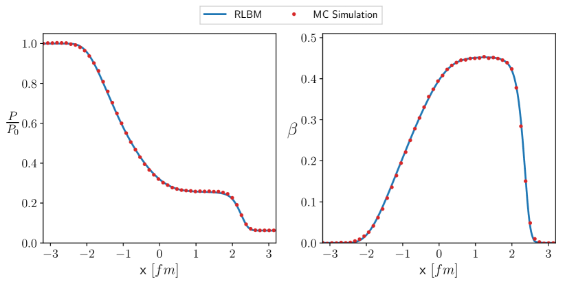
Figure 15: Sod’s shock tube for a gas of massive particles $(m=800~{}\rm{MeV})$ at $t=3.2~{}\rm{fm/c}$, at $\eta/s=1/2\pi$. The results of simulations of the RLBM (lines) are compared with those obtained solving the RBE with a Monte Carlo approach. Left: pressure profile. Right) $\beta=|U^{i}|/U^{0}$. RLBM simulations have been performed on grids of size $6400\times 1\times 1$, using a third order quadrature identified by the velocity set $G_{\rm C}^{(\rm o3)}$ in Table 3.

When a non-zero viscosity is introduced, dissipation smoothens the interfaces between the different regions. Since in the viscous regime it is not possible to provide an exact solution, we compare with the results of other numerical solvers, such as the Boltzmann approach multi-parton scattering program (BAMPS) [96, 97].

The initial conditions in this case are: $P_{\rm L}=5.43~{}\rm{GeV/fm^{3}}$, $P_{\rm R}=0.339~{}\rm{GeV/fm^{3}}$, $T_{\rm L}=400~{}\rm{MeV}$ and $T_{\rm R}=200~{}\rm{MeV}$. We use a $(3+1)$-dimensional EOS, and the same relation for the entropy density used in BAMPS: $s=4n-n\ln{(n/n^{\rm eq})}$, where $n^{\rm eq}$ comes from the equilibrium function, $n^{\rm eq}=d_{\rm G}T^{3}/\pi^{2}$, with $d_{\rm G}=16$ the degeneracy of the gluons [98].

In Fig. 14 we present the results of simulations for a few selected values of $\eta/s$, corresponding to different viscous regimes: $\eta/s=0.002$ is the nearly inviscid hydrodynamic regime discussed above, a highly viscous flow at $\eta/s=0.1$ where an hydrodynamic approach is still justified, and finally $\eta/s=0.5$ where we enter a transition towards a ballistic regime (thus going beyond hydrodynamics). For $\eta/s=0.1$ the RLBM simulation is in excellent agreement with the results provided by BAMPS. Here we can observe that as the viscosity is increased, the interfaces between the different regions becomes smoother, and eventually cannot be distinguished anymore when we move to $\eta/s=0.5$: in this last example we are transitioning towards a ballistic regime, where the hydrodynamic approach becomes questionable.

We conclude this section taking into consideration relativistic shock waves for fluids of massive particles, a setup which has been rarely addressed in previous studies [9]. Lacking an analytical solution to the problem, we compare the results of RLBM simulations against the results produced by another numerical solver, which solves the full relativistic Boltzmann equation using a Monte-Carlo approach based on the test-particles method [99, 100, 101, 102]. In Fig. 15 we show an example for a gas of particles of mass $m=800~{}\rm{MeV}$ and the same initial conditions used in the previous case: $T_{\rm L}=400~{}\rm{MeV}$, $T_{\rm R}=200~{}\rm{MeV}$, $P_{\rm L}=5.43~{}\rm{GeV/fm^{3}}$ and $P_{\rm R}=0.339~{}\rm{GeV/fm^{3}}$. The ratio $\eta/s$ is kept fixed to the value $1/2\pi$. We appreciate an excellent agreement in both the pressure and velocity profiles. A more detailed analysis will be reported elsewhere.

8.3 Quark-gluon plasma

The study of quark-gluon plasma is the most natural application ground for the RLBM. In this section, we provide a very preliminary example in which we simulate the evolution of the initial stages of heavy-ion collisions. We consider the same numerical setup used in [103], with an initial Gaussian distribution for the temperature profile

$$T=T_{\rm r}~{}g(x,y,z),\quad g(x,y,z)=\exp{(-\frac{x^{2}}{2\sigma_{x}^{2}}-\frac{y^{2}}{2\sigma_{y}^{2}}-\frac{z^{2}}{2\sigma_{z}^{2}})}\quad,$$ (93)

and likewise for the particle density $n=n_{\rm r}~{}g(x,y,z)$.

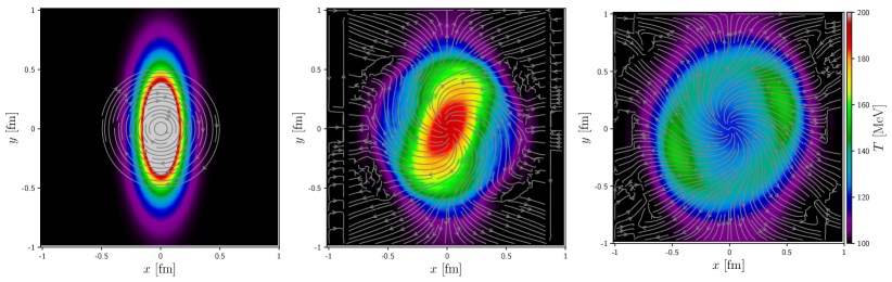
Figure 16: Temperature profile of the system in the $x-y$ plane at $z=0~{}{\rm fm}$, at three different time steps, from left to right $t=0~{}{\rm fm/c},t=0.35~{}{\rm fm/c},t=0.7~{}{\rm fm/c}$. White lines represent the velocity streamlines of the fluid.

The initial temperature at the center of the fireball is $T_{\rm r}=200~{}{\rm MeV}$, with $n_{\rm r}=1.25~{}{\rm fm^{-3}}$, and the particles mass $m=1~{}{\rm GeV}$. We also add a background temperature of $T=100~{}{\rm MeV}$ and density of $n_{\rm r}=0.625~{}{\rm fm^{-3}}$ to avoid numerical instabilities far from the center of the fireball, where we would have a zero temperature which cannot be sustained by the RLBM solver.

The initial velocity profile is given by

$$U^{\alpha}=\gamma\left(1,-h(r)y,h(r)x,0\right),\quad h(r)=\frac{1}{r}\tanh{(\frac{r}{r_{0}})}$$ (94)

with $r$ the distance from the center of the fireball, and $r_{0}$ a parameter describing the strength of the flow. We take $r_{0}=1~{}{\rm fm}$.

Under these initial conditions, the evolution of the system is triggered by an initial rotation around the $z$ axis. In Fig. 16 we show the temperature profile of the system in the x-y plane at $z=0~{}{\rm fm}$, at three different time steps. We can see that the symmetry of the rotating ellipsoid is quickly broken, with the single source splitting into two separate hot spots. The evolution is qualitatively similar to the one portrayed in [103], with a more quantitative analysis left to future detailed work.

8.4 Hydrodynamic flow of electrons in graphene

We now take into consideration an “exotic” application of dissipative relativistic hydrodynamics and apply the RLBM to the study of the dynamics of the electrons in graphene sheets. The motivation for adopting these type of solvers comes from the fact that electrons in graphene sheets follow an ultra-relativistic dispersion relation, so they can be regarded as a fluid of massless (quasi-) particles whose energy depends on momentum as $\epsilon_{\rm F}=v_{\rm F}|\bm{p}|$, with the Fermi speed $v_{\rm F}\sim 10^{6}m/s$ mimicking the role of the speed of light in true relativistic systems.

In this section we provide a validation of this numerical approach by simulating steady-state flows in the so-called ”vicinity-geometry”, which has been subject of several theoretical and experimental studies [104, 105, 106] to outline phenomena such as negative nonlocal resistance, current whirlpools, and measuring the Hall viscosity of graphene’s electrons fluid. The geometrical setup is sketched in Fig. 18, which represents a single-layer graphene sheet of dimension $L\times W$ (usually encapsulated between one or more layers of dielectric materials, such as boron nitride), in which two electrodes are used to inject and drain a constant current within the device.

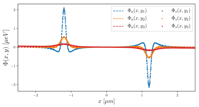
Figure 17: Electrochemical potential measured at several fixed distances from the side of the graphene sample, respectively $y_{1}=0.1~{}\rm{\mu m}$, $y_{2}=0.2~{}\rm{\mu m}$, $y_{3}=0.4~{}\rm{\mu m}$. With $\Phi_{s}(x,y)$ we indicate the results of a numerical simulation, which are compared with the analytic solution $\Phi_{a}(x,y)$ for the benchmark (Eq. 95).

Experimental measurements have shown voltage drops in the proximity of the injectors, which are found to be dependent on the viscosity of the electron fluid [104]. An accurate analytic approximation of the experimental results for the electrochemical potential is derived in the same paper:

$$\Phi(x,y)=\frac{m\nu I}{\bar{n}e^{2}W^{2}}\left[F_{2}(x-x_{0},y)-F_{2}(x+x_{0},y)\right]\quad,$$ (95)

where for single layer graphene the effective mass $m$ is defined as $m=\epsilon_{\rm F}/v_{\rm F}^{2}$, $I$ is the magnitude of the injected current, $\bar{n}$ the equilibrium density, $W$ the width of the device, $e$ the elementary charge, $\nu$ the kinematic viscosity, and

$$F_{2}(x,y)=\pi\frac{1+\cosh(\pi x/W)\cos(\pi y/W)}{\left[\cosh(\pi x/W)\cos(\pi y/W)\right]^{2}}\quad.$$ (96)

The expression above has been obtained by assuming an infinitely long sample. In our simulations, we use a grid with aspect ratio $L/W=4$. Regarding boundary conditions, current is set to zero at the boundaries of the sample, while the equilibrium value of the distribution is imposed at the grid points used to represent the contacts [17].

Since $\Phi$ is not a direct observable of our lattice formulation, we need to perform a parameter matching procedure (see [55] for details) in order to compare with Eq. 95:

$$\Phi(x,y)=\varphi(x,y)-\frac{\delta P(x,y)}{e\bar{n}}\quad,$$ (97)

where $\varphi({\bm{r}},t)$ is the electrical potential self-induced by the electrons motion withing the $2d$ graphene layer, and $\delta P(x,y)\approx T(x,y)(n(x,y)-\bar{n}(x,y))$ is the local pressure difference. Fig. 17 compares our simulation against the analytical prediction of Eq. 95, showing very good agreement at several distances from the boundary layer.

For a treatment of the problem closer to the experimental setup, it is important to include not only effects due to electric forces but also interactions with phonons and impurities. To this end, we have included an external forcing term:

$$\bm{F}=-e\nabla\varphi-\frac{1}{\tau_{\rm D}}n\bm{u}\quad;$$ (98)

the first term is the contribution due to the electric field, which in principle would require the solution of the full Poisson equation; since this approach is computationally expensive, we compute $\varphi(x,y)$ by employing a local capacitance approximation [107]:

$$\varphi(x,y)=-\frac{e}{C_{\rm g}}\bar{n}(x,y)\quad,$$ (99)

with $C_{g}$ the geometrical capacitance per unit area, depending on both the geometrical and permittivity properties of the dielectric layer. The second term in Eq. 98 is used to parametrize phonon-electron scattering as a friction term, with $\tau_{\rm D}$ the single scattering time. Albeit very simple, this parametrization has proven successful in describing experiments in the linear-response regime [108, 109, 110].

\begin{overpic}[width=401.09981pt]{fig18a} \put(46.0,15.0){$W$} \put(49.0,1.5){$L$} \end{overpic}

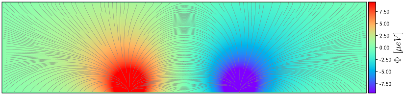
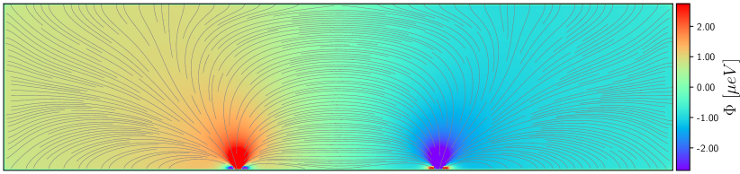
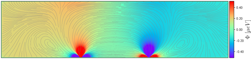
Figure 18: a) Sketch of the ”vicinity-geometry” used in simulations: Two contacts are used to inject (red area) and drain (green area) a current from a graphene sheet of width $W$. The current is zero at the boundaries of the sample (black areas). b-d) Snapshot of three different simulations at the steady-state, all using $W=2\mu m$, $\bar{n}=2\cdot 10^{-12}~{}\rm cm^{-2}$, $I=10^{-7}~{}\rm A$, $\nu=0.005~{}m^{2}/s$ and $C_{g}/e^{2}=3.03\cdot 10^{35}~{}J^{-1}m^{-2}$, and for different values of $\tau_{\rm D}$. In b) $\tau_{\rm D}=1~{}\rm{ps}$, in c) $\tau_{\rm D}=20~{}\rm{ps}$, in d) $\tau_{\rm D}=200~{}\rm{ps}$ The color map describes the electrochemical potential. Lines represent the electrons velocity streamlines.

In Fig. 18 we show a few examples which qualitatively summarize the results of the simulations. The simulations are conducted using the following physical parameter: $W=2\mu m$, $\bar{n}=2\cdot 10^{-12}~{}\rm cm^{-2}$, $I=10^{-7}~{}\rm A$, $\nu=0.005~{}m^{2}/s$ and $C_{g}/e^{2}=3.03\cdot 10^{35}~{}J^{-1}m^{-2}$. In panel b), we show a simulation with $\tau_{D}=1~{}\rm ps$, in which the interaction with phonons is sufficiently strong to prevent the onset of a hydrodynamic regime. In panel c), we show the result of a simulation with $\tau_{D}=20~{}\rm ps$, where we observe a weak signature of a hydrodynamic behavior in the proximity on the current injector (note the formation of a negative potential). Finally in panel d) we show that for $\tau_{D}=200~{}\rm ps$ we observe the formation of current whirlpools.

For the geometric setup here analyzed the authors in [105] predicted the formation of backflow near the injectors for arbitrarily small values of the vorticity diffusion parameter $D_{\nu}=\sqrt{\nu\tau_{\rm D}}$. However, for similar geometries they also found that the transition occurs when a specific threshold is overrun, i.e. $D_{\nu}>W/(\sqrt{2}\pi)$, which can be expressed in a more explicit form as

$$\nu>\nu_{*}=\frac{W^{2}}{2\pi^{2}~{}\tau_{D}}\quad.$$ (100)

The above expression is in good agreement with our simulations since for the parameters used in panel b) we get $\nu_{*}\approx 0.2~{}\rm m^{2}/s$, for panel c), where we observe the first signatures of the hydrodynamic regime we have $\nu_{*}\approx 0.01~{}\rm m^{2}/s$, thus a figure about the same order of magnitude of the actual viscosity, and finally $\nu_{*}\approx 0.001~{}\rm m^{2}/s$ for the parameters used in the simulation corresponding to panel d).

9 Conclusions

This paper has presented an exhaustive account of the conceptual and mathematical development of a suite of Lattice Boltzmann methods capable of describing relativistic dissipative fluid flows over a wide kinematic range, ranging from ultra-relativistic ($\zeta\to 0$) to near non-relativistic ($\zeta\rightarrow\infty$), and – in principle – in any number of space dimensions. All these methods are based on the expansion of the Jüttner distribution onto an appropriate basis of orthogonal polynomials and on its discretization, via Gauss-like quadrature, on a regular and uniform lattice. Quadratures have been studied up to the fifth order, even though – on computational efficiency grounds – only the third order can be tackled in practice. While building largely on previous developments, the present work considerably streamlines previous formulations with a uniform treatment of all spatial dimensions.

The main advantage of the kinetic approach to relativistic hydrodynamics is to ensure built-in relativistic covariance and causality also in the presence of dissipative effects. This is welcome but still leaves an open question as to the connection between the meso-scale relaxation time and the macroscopic transport coefficients. This problem is as practical as it is conceptual, since different theoretical treatments yield different results in the relativistic regime; several recent developments suggest that the Chapman Enskog expansion as the correct route. It would be obviously interesting to have this result confirmed by a carefully planned experimental setup, hopefully to be available in the coming years. Meanwhile, this work provides a neat numerical answer: we have compared in detail the predictions of the CE approach and of Grad’s moment and gathered convincing numerical evidence that, in $1$, $2$ and $3$ spatial dimensions, the CE approach is the one correctly linking all macroscopic transport coefficients, $\lambda$, $\eta$ and $\mu$ to the mesoscopic relaxation time $\tau$. This solves the problem in the relaxation-time approximation but, given the universal nature of the macroscopic coefficients, strongly suggests that this is likely to offer the correct path also for more complex formulations of the Boltzmann equation.

In any case, the analysis described above provides a neat and accurate calibration procedure that enables the present RLB scheme for the simulation of a variety of relativistic hydrodynamic problems.

The computational framework derived from the present RLB method has been extensively validated in several contexts where analytical results or semi-analytical approximations are available, and over a broad range of kinematic regimes. Our tests also include an ”exotic” application to the electron dynamics in graphene sheets, opening the way to accurate and realistic numerical simulations of these materials.

We have made a specific effort to describe in detail all steps of our derivations and results, so as to allow the interested reader to reproduce them.

The RLB method can hopefully find potential use for a wealth of different relativistic fluid problems across scales, from astrophysics and cosmology to high-energy physics and material science.

Much is left for the future. At the methodological level, new lines of development may include – in the short time frame – comparison with different solvers, with a close eye on the trade-off between computational efficiency and physical accuracy, development of accurate boundary conditions, and – on a longer time frame – an analysis of the relevance of quantum effects, as described for instance by quantum versions of the Maxwell-Jüttner distribution. Moreover, off-lattice scheme could represent an efficient solution to further extend the parameter regimes supported by the method, allowing covering BH-regimes, and fluids consisting of particles of vanishingly-small non-zero mass.

As to applications, the customization of the RLB scheme to the detailed study of quark-gluon plasmas dynamics in current and future high-energy experiments, appears a very appealing topic for future research.

Appendix A Notation

In this appendix we summarize the notation used throughout this work. We also introduce useful projector operators, including some of their relevant properties, which have been often used in the main text and on which we extensively rely for the calculation of the transport coefficients.

We work in a flat (d+1) dimensional space-time, parametrized by the coordinates

$$\left(x^{\alpha}\right)=\left(ct,\bm{x}\right)\quad,$$ (101)

with the first component giving the time coordinate, while the second term represents the usual spatial coordinates in a $d$ dimensional Euclidean space.

The notation $\left(A^{\alpha}\right)$ is used to represent a vector $\in\mathbb{R}^{d+1}$ (for simplicity, we refer to these vectors as four vectors in the text, even when $d\neq 3$) while the boldface notation $\bm{A}$ is used for vectors $\in\mathbb{R}^{d}$. Greek indexes are used to denote $(d+1)$ space-time coordinates and Latin indexes for $d$ dimensional spatial coordinates. Einstein’s summation convention over repeated indexes is adopted.

We use the metric tensor $\eta^{\alpha\beta}=diag(1,-\mathds{1})$, with $\mathds{1}=\left(1,\dots,1\right)\in\mathbb{N}^{d}$.

The Minkowski-orthogonal projector to the fluid velocity $U^{\alpha}$ is defined as

$$\Delta^{\alpha\beta} =\eta^{\alpha\beta}-\frac{1}{c^{2}}U^{\alpha}U^{\beta}\quad,$$ (102)

$$\Delta_{\alpha\beta} =\eta_{\alpha\beta}-\frac{1}{c^{2}}U_{\alpha}U_{\beta}\quad.$$ (103)

By construction, the product of $\Delta_{\alpha\beta}$ with the quadri-velocity $U^{\beta}$ is therefore equal to zero, and its trace equals the number of spatial dimensions:

$$\Delta^{\alpha\beta}U_{\beta} =\Delta_{\alpha\beta}U^{\beta}=0\quad,$$ (104)

$$\Delta^{\alpha}_{\alpha} =d\quad.$$ (105)

It is useful to introduce the short-hand notation

$$\Delta^{\alpha}_{\gamma}=\Delta^{\alpha\beta}\Delta_{\beta\gamma}=\delta^{\alpha}_{\gamma}-\frac{1}{c^{2}}U^{\alpha}U_{\gamma}\quad,$$ (106)

together with the following easily verifiable properties:

$$\Delta_{\alpha}^{\gamma}\Delta_{\gamma\beta} =\Delta_{\alpha\beta}\quad,$$ (107)

$$\Delta^{\alpha}_{\gamma}\Delta^{\gamma}_{\beta} =\Delta^{\alpha}_{\beta}\quad.$$ (108)

These projectors can be applied to express a generic quadri-vector $A^{\alpha}$ as the sum of two terms, respectively orthogonal and parallel to $U^{\alpha}$:

$$A^{\alpha}=\Delta^{\alpha\beta}A_{\beta}+\frac{1}{c^{2}}U^{\alpha}U^{\beta}A_{\beta}\quad.$$ (109)

Likewise, we can decompose a generic tensor $T^{\alpha\beta}$ in order to identify the symmetric $U^{\alpha}$-orthogonal components $T^{(\alpha\beta)}$:

$$T^{(\alpha\beta)}=\frac{1}{2}\left(\Delta^{\alpha}_{\gamma}\Delta^{\beta}_{\delta}+\Delta^{\beta}_{\gamma}\Delta^{\alpha}_{\delta}\right)T^{\gamma\delta}=\frac{1}{2}\left(\Delta^{\alpha\gamma}\Delta^{\beta\delta}+\Delta^{\beta\gamma}\Delta^{\alpha\delta}\right)T_{\gamma\delta}\quad,$$ (110)

the antisymmetric $U^{\alpha}$-orthogonal components $T^{[\alpha\beta]}$:

$$T^{[\alpha\beta]}=\frac{1}{2}\left(\Delta^{\alpha}_{\gamma}\Delta^{\beta}_{\delta}-\Delta^{\beta}_{\gamma}\Delta^{\alpha}_{\delta}\right)T^{\gamma\delta}=\frac{1}{2}\left(\Delta^{\alpha\gamma}\Delta^{\beta\delta}-\Delta^{\beta\gamma}\Delta^{\alpha\delta}\right)T_{\gamma\delta}\quad,$$ (111)

and the symmetric, traceless, $U^{\alpha}$-orthogonal components $T^{<\alpha\beta>}$:

$$T^{<\alpha\beta>}=T^{(\alpha\beta)}-\frac{1}{d}\Delta^{\alpha\beta}\Delta_{\gamma\delta}T^{(\gamma\delta)}\quad.$$ (112)

The following properties naturally follow from the definitions above:

$$U_{\alpha}T^{(\alpha\beta)} =0 \eta_{\alpha\beta}T^{(\alpha\beta)} =\Delta_{\mu\nu}T^{\mu\nu} \Delta_{\alpha\beta}T^{(\alpha\beta)} =\Delta_{\mu\nu}T^{\mu\nu}\quad,$$ (113)

$$U_{\alpha}T^{[\alpha\beta]} =0 \eta_{\alpha\beta}T^{[\alpha\beta]} =0 \Delta_{\alpha\beta}T^{[\alpha\beta]} =0\quad,$$ (114)

$$U_{\alpha}T^{<\alpha\beta>} =0 \eta_{\alpha\beta}T^{<\alpha\beta>} =0 \Delta_{\alpha\beta}T^{<\alpha\beta>} =0\quad.$$ (115)

It is at times useful to introduce a decomposition also for the quadri-gradient $\partial_{\alpha}$, by defining the convective time derivative $D$ and its orthogonal component $\nabla^{\alpha}$:

$$\partial^{\alpha}=\Delta^{\alpha\beta}\partial_{\beta}+\frac{1}{c^{2}}U^{\alpha}U^{\beta}\partial_{\beta}=\nabla^{\alpha}+\frac{1}{c^{2}}U^{\alpha}D\quad,$$ (116)

with the following useful properties:

$$U_{\alpha}\nabla^{\alpha} =0\quad,$$ (117)

$$\nabla^{\alpha}U_{\alpha} =\partial^{\alpha}U_{\alpha}\quad.$$ (118)

Appendix B Integrals of the Maxwell-Jüttner distribution

We compute here some integrals often used in the development of the numerical methods presented in this work and in the definition of the transport coefficients.

B.1 Integrals $Z^{\alpha_{1}\dots\alpha_{n}}$

Let

$$Z= \int e^{-\frac{p_{\mu}U^{\mu}}{k_{\rm B}T}}\frac{\mathop{}\!\mathrm{d}^{d}p}{p_{0}}$$ (119)

$$Z^{\alpha_{1}\dots\alpha_{n}}= \int e^{-\frac{p_{\mu}U^{\mu}}{k_{\rm B}T}}p^{\alpha_{1}}\dots p^{\alpha_{n}}\frac{\mathop{}\!\mathrm{d}^{d}p}{p_{0}}\quad.$$ (120)

$Z^{\alpha_{1}\dots\alpha_{n}}$ is obtained via differentiation of $Z$ with respect to $U_{\alpha_{1}}\dots U_{\alpha_{n}}$:

$$Z^{\alpha_{1}\dots\alpha_{n}}=(-k_{\rm B}T)^{n}\frac{\partial Z}{\partial U_{\alpha_{1}}\dots\partial U_{\alpha_{n}}}\quad.$$ (121)

$Z$ is a Lorentz-invariant quantity which depends only on $U_{\alpha}U^{\alpha}=c^{2}$; however, as we need to compute derivatives with respect to $U^{\alpha}$, we first derive the result for an unconstrained $U_{\alpha}U^{\alpha}$ and, after performing the derivatives, evaluate the result for $U_{\alpha}U^{\alpha}=c^{2}$.

We write:

$$Z=\int e^{-\frac{p_{0}\sqrt{U^{\mu}U_{\mu}}}{k_{\rm B}T}}\frac{d^{d}p}{p_{0}}=\int e^{-\frac{\sqrt{U^{\mu}U_{\mu}}}{k_{\rm B}T}\sqrt{m^{2}c^{2}+p^{2}}}\frac{d^{d}p}{\sqrt{m^{2}c^{2}+p^{2}}}\quad,$$ (122)

and then switch to spherical coordinates:

$$d^{d}p=p^{d-1}dp~{}d\Omega \int d\Omega=\frac{d\pi^{\frac{d}{2}}}{\Gamma\left(1+\frac{d}{2}\right)}\quad,$$ with

giving

$$Z=\frac{d\pi^{\frac{d}{2}}}{\Gamma\left(1+\frac{d}{2}\right)}\int_{0}^{+\infty}e^{-\frac{\sqrt{U^{\mu}U_{\mu}}}{k_{\rm B}T}\sqrt{m^{2}c^{2}+p^{2}}}\frac{p^{d-1}dp}{\sqrt{m^{2}c^{2}+p^{2}}}\quad.$$

Changing integration variable $p=mc\sqrt{t^{2}-1}$ and defining $\zeta=mc^{2}/k_{B}T$, we have

$$Z=\frac{d\pi^{\frac{d}{2}}}{\Gamma\left(1+\frac{d}{2}\right)}(mc)^{d-1}\int_{1}^{+\infty}(t^{2}-1)^{\frac{d-1}{2}-\frac{1}{2}}e^{-\frac{\zeta t}{c}\sqrt{U^{\mu}U_{\mu}}}dt\quad.$$

Recalling one useful definition of the modified Bessel function of the second kind [111]:

$$K_{\nu}(z)=\frac{\pi^{1/2}(z/2)^{\nu}}{\Gamma\left(\nu+1/2\right)}\int_{1}^{+\infty}e^{-zt}(t^{2}-1)^{\nu-1/2}dt\quad,$$

we finally obtain:

$$Z=\pi^{\frac{d-1}{2}}2^{\frac{d+1}{2}}\zeta^{\frac{d-1}{2}}\left(\frac{k_{\rm B}T}{\sqrt{c}}\right)^{d-1}\frac{K_{\frac{d-1}{2}}\left(\frac{\zeta}{c}\sqrt{U^{\mu}U_{\mu}}\right)}{(U^{\mu}U_{\mu})^{\frac{d-1}{4}}}\quad.$$

All integrals can now be obtained using Eq. 121; tedious but straightforward manipulations yield a nice and regular structure. Indeed, defining the coefficients $A_{n}$:

$$A_{n}=2^{\frac{d+1}{2}}\pi^{\frac{d-1}{2}}\zeta^{n+\frac{d-1}{2}}K_{n+\frac{d-1}{2}}(\zeta)\quad,$$ (123)

one obtains:

$$Z= \left(\frac{k_{\rm B}T}{c}\right)^{d-1}A_{0}$$

$$Z^{\alpha}= \left(\frac{k_{\rm B}T}{c}\right)^{d}A_{1}\frac{U^{\alpha}}{c}$$

$$Z^{\alpha\beta}= \left(\frac{k_{\rm B}T}{c}\right)^{d+1}\left[A_{2}\frac{U^{\alpha}U^{\beta}}{c^{2}}-A_{1}\eta^{\alpha\beta}\right]$$

$$Z^{\alpha\beta\gamma}= \left(\frac{k_{\rm B}T}{c}\right)^{d+2}\left[A_{3}\frac{U^{\alpha}U^{\beta}U^{\gamma}}{c^{3}}-A_{2}\left(\frac{\eta^{\alpha\beta}U^{\gamma}+\eta^{\gamma\beta}U^{\alpha}+\eta^{\alpha\gamma}U^{\beta}}{c}\right)\right]$$

$$\dots$$

$$Z^{\alpha_{1}\alpha_{2}\dots\alpha_{n}}= \left(\frac{k_{\rm B}T}{c}\right)^{d+n-1}\sum_{k=0}^{\lfloor\frac{n}{2}\rfloor}(-1)^{k}A_{n-k}\frac{\prec U_{n-2k}\eta_{k}\succ}{c^{n-2k}}$$

Where

$$\prec U_{n-2k}\eta_{k}\succ=\underbrace{\eta^{\alpha_{1}\alpha_{2}}\dots\eta^{\alpha_{2k-1}\alpha_{2k}}}_{\tiny\text{k terms}}\underbrace{U^{\alpha_{2k+1}}U^{\alpha_{2k+2}}\dots U^{\alpha_{n}}}_{\tiny\text{(n-2k) terms}}+\mbox{permutations of indexes}.$$

In the above, terms like $\eta^{\alpha\beta}$, $\eta^{\beta\alpha}$ and $U^{\alpha}U^{\beta}$, $U^{\beta}U^{\alpha}$ are counted only once. To give an example, for $n=4$, $k=1$, we have:

$$\prec U_{2}\eta_{1}\succ =\eta^{\alpha_{1}\alpha_{2}}U^{\alpha_{3}}U^{\alpha_{4}}+\eta^{\alpha_{1}\alpha_{3}}U^{\alpha_{2}}U^{\alpha_{4}}+\eta^{\alpha_{2}\alpha_{3}}U^{\alpha_{1}}U^{\alpha_{4}}$$

$$+\eta^{\alpha_{1}\alpha_{4}}U^{\alpha_{3}}U^{\alpha_{2}}+\eta^{\alpha_{4}\alpha_{3}}U^{\alpha_{2}}U^{\alpha_{1}}+\eta^{\alpha_{2}\alpha_{4}}U^{\alpha_{1}}U^{\alpha_{3}}\quad.$$

B.2 Integrals $K^{\alpha_{1}\dots\alpha_{n}}$

Let

$$K^{\alpha_{1}\dots\alpha_{n}}=\int f^{\rm eq}\frac{p^{\alpha_{1}}\dots p^{\alpha_{s}}}{p_{\mu}U^{\mu}}\frac{\mathop{}\!\mathrm{d}^{d}p}{p_{0}}=B(n,T)\int e^{-\frac{p_{\mu}U^{\mu}}{k_{\rm B}T}}\frac{p^{\alpha_{1}}\dots p^{\alpha_{s}}}{p_{\mu}U^{\mu}}\frac{\mathop{}\!\mathrm{d}^{d}p}{p_{0}}\quad,$$ (124)

with $B(n,T)$ defined in Eq. 11. We include this normalization factor as these integrals are only encountered in the derivation of the transport coefficients following the Chapman-Enskog expansion. It immediately follows from the definition that:

$$U_{\alpha_{n}}K^{\alpha_{1}\dots\alpha_{n}}=B(n,T)Z^{\alpha_{1}\dots\alpha_{n-1}}\quad.$$ (125)

The tensorial structure of $K^{\alpha_{1}\dots\alpha_{n}}$ is similar to that of $Z^{\alpha_{1}\dots\alpha_{n}}$:

$$K^{\alpha} =\frac{n}{ck_{\rm B}T}a_{11}U^{\alpha}$$

$$K^{\alpha\beta} =\frac{n}{c}\left[a_{21}\frac{U^{\alpha}U^{\beta}}{c^{2}}-a_{22}\eta^{\alpha\beta}\right]$$

$$K^{\alpha\beta\gamma} =\frac{nk_{\rm B}T}{c^{2}}\left[a_{31}\frac{U^{\alpha}U^{\beta}U^{\gamma}}{c^{3}}-a_{32}\left(\frac{\eta^{\alpha\beta}U^{\gamma}+\eta^{\gamma\beta}U{\alpha}+\eta^{\alpha\gamma}U^{\beta}}{c}\right)\right]$$

$$\dots$$

$$K^{\alpha_{1}\dots\alpha_{n}} =\frac{n(k_{\rm B}T)^{n-2}}{c^{n-3}}\sum_{k=0}^{\lfloor\frac{n}{2}\rfloor}(-1)^{k}a_{n(k+1)}\frac{\prec U_{n-2k}\eta_{k}\succ}{c^{n-2k}}$$

with (limiting ourselves to up to 4 Lorentz indexes):

$$a_{11} =\frac{1}{\zeta^{2}}\left(G_{d}-(d+1)\right)$$

$$a_{21} =1+\chi a_{22}=\chi$$

$$a_{31} =G_{d}+2 a_{32}=1$$

$$a_{41} =\frac{3G_{d}-3\zeta^{2}\chi}{d+2}+(d+6)G_{d}+\zeta^{2} a_{42}=\frac{(3d+7)G_{d}-\zeta^{2}\chi}{d+2} a_{43}=\frac{G_{d}-\zeta^{2}\chi}{d+2}\quad;$$

$G_{d}$ is defined in Eq. 13 and $\chi$ is:

$$\chi=\left\{\begin{array}[]{ll}\frac{1}{d!!}\sum_{k=0}^{\lfloor\frac{d-1}{4}\rfloor}\zeta^{2k}\left(g^{(k+1)}_{\frac{d+1}{2}-2k}-G_{d}~{}g^{(k+1)}_{\frac{d+1}{2}-2k-1}+(-1)^{\frac{d+1}{2}}\zeta^{\frac{d-1}{2}}\frac{Ki_{1}(\zeta)}{K_{\frac{d+1}{2}}(\zeta)}\right)&\mbox{for odd d}\\ \frac{1}{d!!}\sum_{k=0}^{\lfloor\frac{d-1}{4}\rfloor}\zeta^{2k}\left(h^{(k+1)}_{\frac{d}{2}-2k}-G_{d}~{}h^{(k+1)}_{\frac{d}{2}-2k-1}+(-1)^{\frac{d}{2}}\zeta^{\frac{d-2}{2}}\sqrt{\frac{\pi}{2}}\frac{\Gamma(0,\zeta)}{K_{\frac{d+1}{2}}(\zeta)}\right)&\mbox{for even d}\end{array}\right.$$

Finally, the coefficients $g^{(i)}_{j}$ and $h^{(i)}_{j}$ are defined as:

$$g^{(i)}_{j}=\begin{cases}0\\ 1\\ 2j~{}g^{(i)}_{j-1}+(2j-3)!!\\ 2(j+2i-2)~{}g^{(i)}_{j-1}+~{}g^{(i-1)}_{j}\end{cases}h^{(i)}_{j}=\begin{cases}0&\mbox{for }j=0\\ 1&\mbox{for }j=1\\ 2j~{}h^{(i)}_{j-1}+(2j-1)!!&\mbox{for }i=1\\ 2(j+2i-\frac{3}{2})~{}h^{(i)}_{j-1}+~{}h^{(i-1)}_{j}&\mbox{else}\\ \end{cases}$$

We write explicitly a few cases:

$$\chi =1-\frac{Ki_{1}}{K_{1}} d=1$$

$$\chi =\frac{1}{2}\left(1-\zeta^{2}\frac{e^{\zeta}\Gamma(0,\zeta)}{1+\zeta}\right) d=2$$

$$\chi =\frac{1}{3}\left(5-G_{d}+\zeta\frac{Ki_{1}}{K_{2}}\right) d=3$$

$$\chi =\frac{1}{8}\left(5-G_{d}+\zeta^{4}\frac{e^{\zeta}\Gamma(0,\zeta)}{\zeta^{2}+3\zeta+3}\right) d=4$$

In the above expressions

$$Ki_{\alpha}=\int_{0}^{\infty}e^{-\zeta\cosh(t)}\left(\cosh(t)\right)^{-\alpha}\mathop{}\!\mathrm{d}t\quad,$$

is the Bickley-Naylor function and

$$\Gamma(\alpha,x)=\int_{x}^{\infty}y^{\alpha-1}e^{-y}\mathop{}\!\mathrm{d}y\quad,$$

is the upper incomplete gamma function.

Appendix C Derivation of transport coefficients

In this appendix section we present the detailed derivation of the transport coefficients for the relativistic Boltzmann equation in the relaxation time approximation. We present the analytical derivation in a general $(d+1)$-dimensional Minkowski space-time following both the Chapman Enskog expansion and Grad’s method of moments. Useful for both cases are the constitutive equations for the heat flux, the dynamic pressure and the pressure deviator, which can be identified by applying suitable projectors, defined in Appendix A, to the non equilibrium components of the first and second order tensors of the particles distribution function (Eq. 22 and Eq. 23). The resulting expressions write as follows:

$$q^{\alpha} =-h_{e}\Delta^{\alpha\beta}N_{\alpha}\quad,$$ (126)

$$\varpi =-P-\frac{1}{d}\Delta_{\alpha\beta}T^{\alpha\beta}\quad,$$ (127)

$$\pi^{<\alpha\beta>} =\Delta^{<\alpha}_{\mu}\Delta^{\beta>}_{\nu}T^{\mu\nu}=\left(\Delta^{\alpha}_{\mu}\Delta^{\beta}_{\nu}-\frac{1}{d}\Delta^{\alpha\beta}\Delta_{\mu\nu}\right)T^{\mu\nu}\quad.$$ (128)

C.1 Chapman-Enskog expansion

The Chapman-Enskog expansion consists in splitting the particle distribution function $f$ in two additive terms: the equilibrium distribution $f^{\rm eq}$ and a non equilibrium part $f^{\rm neq}$. When working in a hydrodynamic regime, it is reasonable to approximate $f^{\rm neq}$ with a small deviation from the equilibrium:

$$f=f^{\rm eq}+f^{\rm neq}\sim f^{\rm eq}(1+\phi)\quad.$$ (129)

with $\phi$ of the order of the Knudsen number $\rm Kn$, defined as the ratio between the mean free path and a typical macroscopic length scale. Before going in details, we briefly outline the conceptual steps of the expansion. The general idea is to determine an analytical expression for the deviation from the equilibrium $f^{\rm eq}\phi$. We start from Eq. 2 (let us ignore for the moment the forcing term), insert Eq. 129 and retain only terms $\mathcal{O}(\rm{Kn})$, giving:

$$p^{\alpha}\partial_{\alpha}f^{\rm eq}=-\frac{p^{\alpha}U_{\alpha}}{c^{2}\tau}f^{\rm eq}\phi\quad.$$ (130)

To derive the transport coefficients we will then proceed with the following steps:

1. Compute the derivative $p^{\alpha}\partial_{\alpha}f^{\rm eq}$ and derive the constitutive equations of a relativistic Eulerian fluid.

2. Use the balance equations for energy and momentum to eliminate the convective time derivatives and derive the analytic expression of $\phi$.

3. Use the now known expression for $f^{\rm eq}\phi$ to compute the first and second order tensors (via their integral definitions), compare against their definition in the Landau frame and work out the expression for the transport coefficients.

C.1.1 Constitutive equations of a relativistic Eulerian fluid

From Eq. 22 and Eq. 23 we infer the following constraints on the particle distribution function:

$$nc^{2} =U^{\alpha}N_{\alpha}=cU^{\alpha}\int f^{\rm eq}p_{\alpha}\frac{\mathop{}\!\mathrm{d}^{d}p}{p_{0}}=cU^{\alpha}\int fp_{\alpha}\frac{\mathop{}\!\mathrm{d}^{d}p}{p_{0}}\quad,$$ (131)

$$\epsilon c^{2} =U^{\alpha}U^{\beta}T_{\alpha\beta}=U^{\alpha}U^{\beta}c\int f^{\rm eq}p_{\alpha}p_{\beta}\frac{\mathop{}\!\mathrm{d}^{d}p}{p_{0}}=U^{\alpha}U^{\beta}c\int fp_{\alpha}p_{\beta}\frac{\mathop{}\!\mathrm{d}^{d}p}{p_{0}}\quad.$$ (132)

These conditions together with Eq. 129 lead to the following constraints for the non-equilibrium part of the distribution:

$$U_{\alpha}\int p^{\alpha}\phi f^{\rm eq}\frac{d^{d}p}{p_{0}} =0\quad,$$ (133)

$$U_{\alpha}U_{\beta}\int p^{\alpha}p^{\beta}\phi f^{\rm eq}\frac{d^{d}p}{p_{0}} =0\quad.$$ (134)

Furthermore, we multiply Eq. 130 by $\{1,p^{\beta}\}$ and integrate in momentum space, getting:

$$\int p^{\alpha}\partial_{\alpha}f^{\rm eq}\frac{d^{d}p}{p_{0}} =-\frac{1}{c^{2}\tau}U_{\alpha}\int p^{\alpha}\phi f^{\rm eq}\frac{d^{d}p}{p_{0}}=0\quad,$$ (135)

$$\int p^{\beta}p^{\alpha}\partial_{\alpha}f^{\rm eq}\frac{d^{d}p}{p_{0}} =-\frac{1}{c^{2}\tau}U_{\alpha}\int p^{\beta}p^{\alpha}\phi f^{\rm eq}\frac{d^{d}p}{p_{0}}=0\quad.$$ (136)

We now use the definition of the Maxwell-Jüttner distribution (Eq. 3) to calculate $p^{\alpha}\partial_{\alpha}f^{\rm eq}$:

$$p^{\alpha}\partial_{\alpha}f^{\rm eq}=f^{\rm eq}p^{\alpha}\left[\frac{\partial_{\alpha}n}{n}+\left(1-G_{d}\right)\frac{\partial_{\alpha}T}{T}\right]+f^{\rm eq}\frac{p^{\alpha}p^{\beta}}{k_{\rm B}T}\left[\frac{U_{\beta}\partial_{\alpha}T}{T}-\partial_{\alpha}U_{\beta}\right]\quad.$$ (137)

Plugging Eq. 137 into Eq. 135 and Eq. 136 gives

$$\left[\frac{\partial_{\alpha}n}{n}+\left(1-G_{d}\right)\frac{\partial_{\alpha}T}{T}\right]Z^{\alpha}+\frac{1}{k_{\rm B}T}\left[\frac{U_{\beta}\partial_{\alpha}T}{T}-\partial_{\alpha}U_{\beta}\right]Z^{\alpha\beta} =0\quad,$$ (138)

$$\left[\frac{\partial_{\alpha}n}{n}+\left(1-G_{d}\right)\frac{\partial_{\alpha}T}{T}\right]Z^{\alpha\beta}+\frac{1}{k_{\rm B}T}\left[\frac{U_{\beta}\partial_{\alpha}T}{T}-\partial_{\alpha}U_{\beta}\right]Z^{\alpha\beta\gamma} =0\quad,$$ (139)

with details on the calculation of integrals $Z^{\alpha_{1}\dots\alpha_{n}}$ given in Appendix B.

It is possible to rearrange the above equations as

$$0 =Dn+n\nabla^{\alpha}U_{\alpha}\quad,$$ (140)

$$0 =-\partial^{\beta}(nT)+n\frac{U^{\beta}DT}{c^{2}}\left[(2+d)G_{d}+\zeta^{2}-G_{d}^{2}\right]+G_{d}nT\frac{DU^{\beta}}{c^{2}}\quad.$$ (141)

The first equation above is immediately recognized as the relativistic counterpart of the continuity equation, while the balance equations for energy and momentum stem from the second equation. To summarize we get:

$$Dn+n\nabla^{\alpha}U_{\alpha} =0\quad,$$ (142)

$$nc_{v}DT+P\nabla_{\alpha}U^{\alpha} =0\quad,$$ (143)

$$\nabla^{\gamma}P-\left(P+\epsilon\right)\frac{DU^{\gamma}}{c^{2}} =0\quad,$$ (144)

where Eq. 143 and Eq. 144 have been derived by multiplying Eq. 141 respectively by $U_{\beta}$ and $\Delta^{\gamma}_{\beta}$, using the EOS in Eq. 14, and having identified the general expression for the heat capacity $c_{v}$ [58]:

$$c_{v}=k_{\rm B}\left[(2+d)G_{d}+\zeta^{2}-G_{d}^{2}-1\right]\quad.$$ (145)

C.1.2 Approximation of the non-equilibrium term of the particle distribution function

Combining Eq. 130 with Eq. 137 it is possible to define an analytic expression for $\phi$. The final result reads as

$$\phi=-\frac{c^{2}\tau}{p^{\mu}U_{\mu}}p^{\alpha}\left[\frac{\partial_{\alpha}n}{n}+\left(1-G_{d}\right)\frac{\partial_{\alpha}T}{T}+p^{\beta}\frac{U_{\beta}\partial_{\alpha}T}{k_{\rm B}T^{2}}-\frac{p^{\beta}\partial_{\alpha}U_{\beta}}{k_{\rm B}T}\right]\quad.$$ (146)

By knowing the deviation of the Maxwell-Jüttner distribution function it is now possible to determine the transport coefficients from the integral definition of the moments of the distribution. We start by taking into consideration the thermal conductivity.

C.1.3 Thermal Conductivity

In order to determine the analytic expression for the thermal conductivity we consider the integral definition of the particle flow tensor together with Eq. 129:

$$N^{\beta} =c\int p^{\beta}f\frac{\mathop{}\!\mathrm{d}^{d}p}{p_{0}}$$

$$=c\int p^{\beta}f^{\rm eq}\frac{\mathop{}\!\mathrm{d}^{d}p}{p_{0}}+c\int p^{\beta}\phi f^{\rm eq}\frac{\mathop{}\!\mathrm{d}^{d}p}{p_{0}}\quad.$$ (147)

We then insert Eq. 146, giving

$$N^{\beta}=cBZ^{\beta}-c^{3}\tau\left[\frac{\partial_{\nu}n}{n}K^{\nu\beta}+\left(1-G_{d}\right)\frac{\partial_{\nu}T}{T}K^{\nu\beta}+\frac{\partial_{\nu}T}{k_{\rm B}T^{2}}BZ^{\beta\nu}-\frac{\partial_{\nu}U_{\delta}}{k_{\rm B}T}K^{\delta\nu\beta}\right]\quad.$$ (148)

Next, we apply to the above equation the projector $\Delta^{\alpha}_{\beta}$, giving

$$\Delta^{\alpha}_{\beta}N^{\beta}=-c^{2}\tau\left[-a_{22}\nabla^{\alpha}n-a_{22}\left(1-G_{d}\right)\frac{n\nabla^{\alpha}T}{T}-\frac{n\nabla^{\alpha}T}{T}+\frac{n}{c^{2}}DU^{\alpha}\right]\quad,$$ (149)

in which we have used the integrals $K^{\alpha_{1}\dots\alpha_{n}}$ defined in Appendix B, together with the definition of the normalization factor $B(n,T)$ from Eq. 11.

Using the balance equations 142, 144 and 143 it is possible to rearrange Eq. 149 as

$$\Delta^{\alpha}_{\beta}N^{\beta}=-nc^{2}\tau\frac{a_{22}G_{d}-1}{T}\left[\nabla^{\alpha}T-\frac{T}{P+\epsilon}\nabla^{\alpha}P\right]\quad.$$ (150)

To conclude, we combine Eq. 150 with Eq. 126, getting:

$$q^{\alpha}=-h_{e}\Delta^{\alpha}_{\beta}N^{\beta}=c^{2}k_{\rm B}n\tau G_{d}\left(a_{22}G_{d}-1\right)\left[\nabla^{\alpha}T-\frac{T}{P+\epsilon}\nabla^{\alpha}P\right]\quad,$$ (151)

from which, by direct comparison with Eq. 25, we conclude that the thermal conductivity $\lambda$ is defined as

$$\lambda=c^{2}k_{\rm B}n\tau G_{d}\left(a_{22}G_{d}-1\right)\quad.$$ (152)

To give a few examples:

$$\lambda =c^{2}k_{\rm B}n\tau G_{d}\left(G_{d}-1-G_{d}\frac{Ki_{1}}{K_{1}}\right) \quad\quad\quad d=1$$

$$\lambda =c^{2}k_{\rm B}n\tau G_{d}\left(\frac{G_{d}}{2}-1-G_{d}\frac{\zeta^{2}e^{\zeta}\Gamma(0,\zeta)}{2(\zeta+1)}\right) \quad\quad\quad d=2$$

$$\lambda =c^{2}k_{\rm B}n\tau G_{d}\left(\frac{G_{d}}{3}(5-G_{d})-1+G_{d}\zeta\frac{Ki_{1}}{3K_{2}}\right) \quad\quad\quad d=3$$

$$\lambda =c^{2}k_{\rm B}n\tau G_{d}\left(\frac{G_{d}}{8}(5-G_{d})-1+G_{d}\frac{\zeta^{4}e^{\zeta}\Gamma(0,\zeta)}{8(\zeta^{2}+3\zeta+3)}\right) \quad\quad\quad d=4$$

In the ultra relativistic limit ($\zeta\rightarrow 0$), the above expression simplifies to

$$\lambda_{\rm ur}=\frac{d+1}{d}c^{2}k_{\rm B}n\tau\quad.$$ (153)

C.1.4 Bulk Viscosity

In order to determine the analytic expression for the bulk viscosity we take the integral definition of the energy-momentum tensor together with Eq. 129:

$$T^{\alpha\beta} =c\int p^{\alpha}p^{\beta}f\frac{d^{d}p}{p_{0}}$$

$$=c\int p^{\alpha}p^{\beta}f^{\rm eq}\frac{\mathop{}\!\mathrm{d}^{d}p}{p_{0}}+c\int p^{\alpha}p^{\beta}\phi f^{\rm eq}\frac{\mathop{}\!\mathrm{d}^{d}p}{p_{0}}\quad.$$ (154)

next, we insert Eq. 146, giving

$$T^{\alpha\beta}=cBZ^{\alpha\beta}-c^{3}\tau\left[\frac{\partial_{\nu}n}{n}K^{\nu\alpha\beta}+(1-G_{d})\frac{\partial_{\nu}T}{T}K^{\nu\alpha\beta}+\frac{\partial_{\nu}T}{k_{\rm B}T^{2}}BZ^{\nu\alpha\beta}-\frac{\partial_{\nu}U_{\delta}}{k_{\rm B}T}K^{\delta\nu\alpha\beta}\right]\quad.$$ (155)

By applying the projector $\Delta_{\alpha\beta}$ and using the results of the integrals $K^{\alpha_{1}\dots\alpha_{n}}$ given in Appendix B, we obtain:

$$\Delta_{\alpha\beta}T^{\alpha\beta}=-dP+\tau d\left[k_{\rm B}TDn+(1-G_{d})nk_{\rm B}DT+G_{d}nk_{\rm B}DT+Pa_{43}(1+\frac{2}{d})\Delta^{\nu}U_{\nu}\right]\quad.$$ (156)

By comparing Eq. 156 with Eq. 127 we directly get

$$\varpi=-\tau\left[k_{\rm B}TDn+(1-G_{d})nk_{\rm B}DT+G_{d}nk_{\rm B}DT+Pa_{43}\left(1+\frac{2}{d}\right)\Delta^{\nu}U_{\nu}\right]\quad.$$ (157)

We then use balance equations 142, 144 and 143 to remove the convective derivatives $Dn$ and $DT$, leading to:

$$\varpi=P\tau\left[\left(1+\frac{k_{\rm B}}{c_{v}}\right)+a_{43}\left(1+\frac{2}{d}\right)\right]\Delta^{\nu}U_{\nu}\quad,$$ (158)

which implies, by direct comparison with Eq. 27, the following expression for the bulk viscosity $\mu$:

$$\mu=P\tau\left[a_{43}\left(1+\frac{2}{d}\right)-\frac{\zeta^{2}-G_{d}^{2}+(d+2)G_{d}}{\zeta^{2}-G_{d}^{2}+(d+2)G_{d}-1}\right]\quad.$$ (159)

To give a few examples:

$$\mu =P\tau\left(\frac{\zeta^{4}+G_{d}^{3}-4G_{d}^{2}+4G_{d}-\zeta^{2}G_{d}^{2}+2\zeta^{2}G_{d}}{-\zeta^{2}+G_{d}^{2}-3G_{d}+1}+\zeta^{2}\frac{Ki_{1}}{K_{1}}\right) \quad d=1$$

$$\mu =P\tau\left(\frac{\zeta^{4}+3\zeta^{2}+2G_{d}^{3}-12G_{d}^{2}+18G_{d}-\zeta^{2}G_{d}^{2}+2\zeta^{2}G_{d}}{4\left(-\zeta^{2}+G_{d}^{2}-4G_{d}+1\right)}+\frac{e^{\zeta}\zeta^{4}\Gamma(0,\zeta)}{4(\zeta+1)}\right) \quad d=2$$

$$\mu =P\tau\left(\frac{5\zeta^{4}+4\zeta^{2}+3G_{d}^{3}-18G_{d}^{2}+30G_{d}+\zeta^{2}G_{d}^{3}-8\zeta^{2}G_{d}^{2}-\zeta^{4}G_{d}+13\zeta^{2}G_{d}}{9\left(-\zeta^{2}+G_{d}^{2}-3G_{d}+1\right)}-\zeta^{3}\frac{Ki_{1}}{9K_{2}}\right) \quad d=3$$

$$\mu =P\tau\left(\frac{\zeta^{4}G_{d}-\zeta^{2}G_{d}^{3}+13\zeta^{2}G_{d}^{2}-35\zeta^{2}G_{d}-8G_{d}^{3}+80G_{d}^{2}-200G_{d}-7\zeta^{4}-25\zeta^{2}}{32\left(-G_{d}^{2}+6G_{d}+\zeta^{2}-1\right)}+\frac{e^{\zeta}\zeta^{6}\Gamma(0,\zeta)}{32(\zeta^{2}+3\zeta+3)}\right) \quad d=4$$

The bulk viscosity of a monoatomic ultra-relativistic gas vanishes independently with respect to the number of spatial dimensions:

$$\mu_{\rm ur}=0\quad.$$ (160)

C.1.5 Shear Viscosity

In order to determine the analytic expression for the shear viscosity $\eta$ we start from the definition of the pressure deviator given in Eq. 128:

$$(\Delta_{\alpha}^{\gamma}\Delta_{\beta}^{\delta}-\frac{1}{d}\Delta^{\gamma\delta}\Delta_{\alpha\beta})T^{\alpha\beta}=\pi^{<\alpha\beta>}\quad.$$ (161)

We can determine the LHS of the above equation by using the same expression for $T^{\alpha\beta}$ previously identified in the calculation of the bulk viscosity (Eq. 155). We split the task in two parts and start by considering the first term of the LHS, which consists in applying the projector $\Delta_{\alpha}^{\gamma}\Delta_{\beta}^{\delta}$ to the energy-momentum tensor:

$$\Delta_{\alpha}^{\gamma}\Delta_{\beta}^{\delta}T^{\alpha\beta} =c\Delta_{\alpha}^{\gamma}\Delta_{\beta}^{\delta}Z^{\alpha\beta}-c^{3}\tau\left[\frac{\partial_{\nu}n}{n}\Delta_{\alpha}^{\gamma}\Delta_{\beta}^{\delta}K^{\nu\alpha\beta}+(1-G_{d})\frac{\partial_{\nu}T}{T}\Delta_{\alpha}^{\gamma}\Delta_{\beta}^{\delta}K^{\nu\alpha\beta}\right.$$

$$~{}~{}~{}~{}~{}~{}~{}~{}~{}~{}~{}~{}~{}~{}~{}~{}~{}~{}~{}~{}~{}~{}~{}~{}~{}~{}~{}~{}\left.+\frac{\partial_{\nu}T}{k_{\rm B}T^{2}}\Delta_{\alpha}^{\gamma}\Delta_{\beta}^{\delta}Z^{\nu\alpha\beta}-\frac{\partial_{\nu}U_{\mu}}{k_{\rm B}T}\Delta_{\alpha}^{\gamma}\Delta_{\beta}^{\delta}K^{\mu\nu\alpha\beta}\right]\quad.$$ (162)

Using the integral definitions in Appendix B we obtain:

$$\Delta_{\alpha}^{\gamma}\Delta_{\beta}^{\delta}T^{\alpha\beta}=-Pd\Delta^{\gamma\delta}+\tau\left[k_{\rm B}TDn\Delta^{\gamma\delta}+nk_{\rm B}DT\Delta^{\gamma\delta}+Pa_{43}(\nabla^{\gamma}U^{\delta}+\nabla^{\delta}U^{\gamma}+\Delta^{\delta\gamma}\partial_{\nu}U^{\nu})\right]\quad.$$ (163)

By using the balance equations for energy and momentum we get

$$\Delta_{\alpha}^{\gamma}\Delta_{\beta}^{\delta}T^{\alpha\beta} =-P\Delta^{\gamma\delta}+P\tau\left[\left(a_{43}-1-\frac{k_{\rm B}}{c_{v}}\right)\Delta^{\delta\gamma}\nabla_{\nu}U^{\nu}+a_{43}(\nabla^{\gamma}U^{\delta}+\nabla^{\delta}U^{\gamma})\right]$$ (164)

$$=-P\Delta^{\gamma\delta}+\mu\Delta^{\delta\gamma}\nabla_{\nu}U^{\nu}+P\tau a_{43}\left[-\frac{2}{d}\Delta^{\delta\gamma}\nabla_{\nu}U^{\nu}+(\nabla^{\gamma}U^{\delta}+\nabla^{\delta}U^{\gamma})\right]\quad.$$

We now consider the second term on the LHS of Eq. 161 and apply the projection $-\frac{1}{d}\Delta^{\gamma\delta}\Delta_{\alpha\beta}$ to the energy momentum tensor, giving:

$$-\frac{1}{d}\Delta^{\gamma\delta}\Delta_{\alpha\beta}T^{\alpha\beta}=\Delta^{\gamma\delta}(P+\varpi)=\Delta^{\gamma\delta}(P-\mu\nabla^{\mu}U_{\mu})\quad.$$ (165)

Putting all the pieces together we get

$$\pi^{<\gamma\delta>}=(\Delta_{\alpha}^{\gamma}\Delta_{\beta}^{\delta}-\frac{1}{d}\Delta^{\gamma\delta}\Delta_{\alpha\beta})T^{\alpha\beta}=P\tau a_{43}\left[\nabla^{\gamma}U^{\delta}+\nabla^{\delta}U^{\gamma}-\frac{2}{d}\Delta^{\delta\gamma}\nabla_{\nu}U^{\nu}\right]\quad.$$ (166)

To conclude, we expand the RHS of Eq. 26:

$$\pi^{<\gamma\delta>}=2\eta\nabla^{<\gamma}U^{\delta>}=\eta\left[\nabla^{\gamma}U^{\delta}+\nabla^{\delta}U^{\gamma}-\frac{2}{d}\Delta^{\delta\gamma}\nabla_{\nu}U^{\nu}\right]\quad.$$ (167)

which we compare with Eq. 166 to identify the analytical expression for the shear viscosity $\eta$:

$$\eta=P\tau a_{43}\quad.$$ (168)

To give a few examples:

$$\eta =\frac{P\tau}{3}\left(G_{d}-\zeta^{2}+\zeta^{2}\frac{Ki_{1}}{K_{1}}\right) \quad\quad\quad d=1$$

$$\eta =\frac{P\tau}{8}\left(2G_{d}-\zeta^{2}+\frac{e^{\zeta}\zeta^{4}\Gamma(0,\zeta)}{\zeta+1}\right) \quad\quad\quad d=2$$

$$\eta =\frac{P\tau}{15}\left(3G_{d}-5\zeta^{2}+G_{d}\zeta^{2}-\zeta^{3}\frac{Ki_{1}}{K_{2}}\right) \quad\quad\quad d=3$$

$$\eta =\frac{P\tau}{48}\left(8G_{d}-7\zeta^{2}+G_{d}\zeta^{2}+\frac{e^{\zeta}\zeta^{6}\Gamma(0,\zeta)}{\zeta^{2}+3\zeta+3}\right) \quad\quad\quad d=4$$

In the ultra relativistic limit ($\zeta\rightarrow 0$), the above expression simplifies to

$$\eta_{\rm ur}=\frac{d+1}{d+2}P\tau\quad.$$ (169)

C.2 Grad’s Method of Moments

The derivation of the transport coefficients following Grad’s method is based on the moments of the particle distribution function $f$. Likewise for the Chapman Enskog procedure, the starting point consists in defining the non-equilibrium part of $f$, which follows from an expansion in the Hilbert Space of momenta around the equilibrium:

$$f=f^{\rm eq}(1+a_{\alpha}p^{\alpha}+a_{\alpha\beta}p^{\alpha}p^{\beta}+\dots)\quad.$$ (170)

Most of the analytical derivation revolves around determining the expansion coefficients $a_{\alpha_{1}\dots\alpha_{N}}$ by imposing suitable constraints on the fields of interest; in the most standard approach one includes the fourteen fields $n,U^{\alpha},T,q^{\alpha},\varpi,\pi^{<\alpha\beta>}$ which are used in the decomposition of the tensors $N^{\alpha}$ and $T^{\alpha\beta}$ (Eq. 22 and Eq. 23). Note that, as already discussed in the main text, it has been shown [19] that this representation is not based on irreducible tensors, and cannot guarantee that the exact form of the expansion coefficients are obtained once the expansion is truncated.

We follow the same procedure described in [58], where the constraints on the fourteen fields stem from the maximization of the entropy density $s$, and consisting of the following steps:

1. Using Lagrange multipliers method, we find an expansion for $f$, in the form of Eq. 170, that extremizes the entropy density $s$, with the constraints given by definition of $N^{\alpha}U_{\alpha}$, $U_{\alpha}T^{\alpha\beta}$ and $U_{\alpha}T^{\alpha<\beta\gamma>}$.

2. Using Grad’s ansatz for $f$ we compute the third order moment $T^{\alpha\beta\gamma}$.

3. The above expression is then plugged into Eq. 2 to determine the non-equilibrium components of the energy-momentum tensor.

4. By applying the projectors $\Delta^{\delta}_{\beta}U_{\gamma}$, $\Delta_{\beta\gamma}$, and $\Delta^{(\delta}_{\beta}\Delta^{\epsilon)}_{\gamma}-\frac{1}{d}\Delta_{\beta\gamma}\Delta^{\delta\epsilon}$ is it then possible to derive the constitutive equations for the heat-flux, dynamic pressure and the pressure deviator. The expressions for the transport coefficients are finally derived by comparison with Eq. 25, Eq. 26, and Eq. 27.

C.2.1 Moments expansion of the particle distribution function

We start from the definition of the entropy per particle $s$ [58]:

$$s[f]=-\frac{k_{\rm B}}{nc}U^{\alpha}\int p_{\alpha}f\ln{f}\frac{d^{d}p}{p_{0}}\quad.$$ (171)

Next, we define the following constraints which follow from the definitions of $U_{\alpha}N^{\alpha}$, $U_{\alpha}T^{\alpha\beta}$ and $U_{\alpha}T^{\alpha<\beta\gamma>}$:

$$g[f] =U_{\alpha}N^{\alpha}-cU_{\alpha}\int p^{\alpha}f\frac{d^{d}p}{p_{0}}\quad,$$ (172)

$$g^{\beta}[f] =U_{\alpha}T^{\alpha\beta}-cU_{\alpha}\int p^{\alpha}p^{\beta}f\frac{d^{d}p}{p_{0}}\quad,$$ (173)

$$g^{<\gamma\beta>}[f] =U_{\alpha}T^{\alpha<\beta\gamma>}-cU_{\alpha}\int p^{\alpha}p^{<\beta}p^{\gamma>}f\frac{d^{d}p}{p_{0}}\quad.$$ (174)

We then apply Lagrange multipliers method, and look for the expression of $f$ that extremizes the functional $F[f]$, defined as

$$F[f]=s[f]-\lambda g[f]-\lambda_{\beta}g^{\beta}[f]-\lambda_{<\gamma\beta>}g^{<\gamma\beta>}[f]\quad,$$ (175)

and from which follows

$$0=\frac{\partial F}{\partial f}=-\int p_{\alpha}U^{\alpha}\left[\frac{k_{\rm B}}{nc}\left(\ln{f}+1\right)+c\left(\lambda+\lambda_{\beta}p^{\beta}+\lambda_{<\gamma\beta>}p^{<\gamma}p^{\beta>}\right)\right]\frac{d^{d}p}{p_{0}}\quad,$$ (176)

$$f=\exp{\left(-1-\frac{nc^{2}}{k_{\rm B}}(\lambda+\lambda_{\beta}p^{\beta}+\lambda_{<\gamma\beta>}p^{<\gamma}p^{\beta>})\right)}\quad.$$ (177)

Since we know that at the equilibrium the above expression needs to reduce to the Maxwell-Jüttner distribution, we can split the coefficients into two parts, the equilibrium (which we label as $(\rm E)$), and the non-equilibrium part (which we label as $(\rm NE)$):

$$\lambda=\lambda^{(\rm E)}+\lambda^{(\rm NE)}\quad,$$ (178)

$$\lambda_{\beta}=\lambda^{(\rm E)}_{\beta}+\lambda^{(\rm NE)}_{\beta}\quad,$$ (179)

$$\lambda_{<\gamma\beta>}=\lambda^{(\rm E)}_{<\gamma\beta>}+\lambda^{(\rm NE)}_{<\gamma\beta>}\quad,$$ (180)

to then write:

$$f =f^{\rm eq}\exp\left(-\frac{nc^{2}}{k_{\rm B}}(\lambda^{(\rm NE)}+\lambda_{\beta}^{(\rm NE)}p^{\beta}+\lambda_{<\gamma\beta>}^{(\rm NE)}p^{<\gamma}p^{\beta>})\right)\quad.$$ (181)

Under the assumption of processes not far from equilibrium ($\lambda^{(\rm NE)}\ll 1$, $\lambda_{\beta}^{(\rm NE)}\ll 1$, $\lambda_{<\gamma\beta>}^{(\rm NE)}\ll 1$) it is possible to linearly expand the exponential:

$$f\sim f^{\rm eq}\left[1-\frac{nc^{2}}{k_{\rm B}}(\lambda^{(\rm NE)}+\lambda_{\beta}^{(\rm NE)}p^{\beta}+\lambda_{<\gamma\beta>}^{(\rm NE)}p^{<\gamma}p^{\beta>})\right]\quad.$$ (182)

Applying the projectors defined in Appendix A, we can decompose the vector $\lambda_{\beta}^{(\rm NE)}$ and the Lagrange coefficients tensor, $\lambda_{\gamma\beta}^{(\rm NE)}$ in the following way:

$$\lambda_{\beta}^{(\rm NE)} =\tilde{\lambda}U_{\beta}+\tilde{\lambda}_{\gamma}\Delta_{\beta}^{\gamma}\quad,$$ (183)

$$\lambda_{<\gamma\beta>}^{(\rm NE)} =\Lambda U_{\gamma}U_{\beta}+\frac{1}{2}\Lambda_{\alpha}(\Delta_{\gamma}^{\alpha}U_{\beta}+\Delta_{\beta}^{\alpha}U_{\gamma})+\Lambda_{\alpha\delta}(\Delta_{\gamma}^{\alpha}\Delta_{\beta}^{\delta}-\frac{1}{d}\Delta^{\alpha\delta}\Delta_{\gamma\beta})\quad.$$ (184)

The expression for Grad’s distribution function now reads as:

$$f=f^{\rm eq} \left[1-\frac{nc^{2}}{k_{\rm B}}\left(\lambda^{(\rm NE)}+\tilde{\lambda}U_{\beta}p^{\beta}+\tilde{\lambda}_{\gamma}\Delta_{\beta}^{\gamma}p^{\beta}+\Lambda U_{\gamma}U_{\beta}p^{\gamma}p^{\beta}\right.\right.$$

$$\left.\left.+\Lambda_{\alpha}\Delta_{\gamma}^{\alpha}U_{\beta}p^{\gamma}p^{\beta}+\Lambda_{\alpha\delta}\Delta_{\gamma}^{<\alpha}\Delta_{\beta}^{\delta>}p^{\gamma}p^{\beta}\right)\right]\quad,$$ (185)

where we have used the identity $\lambda_{<\gamma\beta>}^{(\rm NE)}p^{<\gamma}p^{\beta>}=\lambda_{<\gamma\beta>}^{(\rm NE)}p^{\gamma}p^{\beta}$.

The next step consists in finding the unknowns $\lambda^{(\rm NE)}$, $\tilde{\lambda}$, $\tilde{\lambda}_{\gamma}$, $\Lambda$, $\Lambda_{\alpha}$, $\Lambda_{\alpha\delta}$. In order to do so, we plug Eq. C.2.1 in the integral definition of $N^{\epsilon}$ and $T^{\mu\nu}$ (Eq. 4 and Eq. 5):

$$N^{\epsilon}=cBZ^{\epsilon}-B\frac{nc^{3}}{k_{\rm B}} \left[\lambda^{(\rm NE)}Z^{\epsilon}+\tilde{\lambda}U_{\beta}Z^{\beta\epsilon}+\tilde{\lambda}_{\gamma}\Delta_{\beta}^{\gamma}Z^{\beta\epsilon}+\Lambda U_{\gamma}U_{\beta}Z^{\epsilon\gamma\beta}\right.$$

$$\left.+\Lambda_{\alpha}\Delta_{\gamma}^{\alpha}U_{\beta}Z^{\epsilon\gamma\beta}+\Lambda_{\alpha\delta}\Delta_{\gamma}^{<\alpha}\Delta_{\beta}^{\delta>}Z^{\epsilon\gamma\beta}\right]\quad,$$ (186)

$$T^{\mu\nu}=cBZ^{\mu\nu}-B\frac{nc^{3}}{k_{\rm B}} \left[\lambda^{(\rm NE)}Z^{\mu\nu}+\tilde{\lambda}U_{\beta}Z^{\beta\mu\nu}+\tilde{\lambda}_{\gamma}\Delta_{\beta}^{\gamma}Z^{\beta\mu\nu}+\Lambda U_{\gamma}U_{\beta}Z^{\mu\nu\gamma\beta}\right.$$

$$\left.+\Lambda_{\alpha}\Delta_{\gamma}^{\alpha}U_{\beta}Z^{\mu\nu\gamma\beta}+\Lambda_{\alpha\delta}\Delta_{\gamma}^{<\alpha}\Delta_{\beta}^{\delta>}Z^{\mu\nu\gamma\beta}\right]\quad,$$ (187)

with integrals $Z^{\alpha_{1}\dots\alpha_{n}}$ computed in appendix B. Combining the above equations with Eq. 131, and Eq. 132, and together with the constitutive equations Eq. 126, Eq. 127, Eq. 128 it is possible to obtain the following linear system of equations for the Lagrange coefficients:

$$\begin{cases}0&=\lambda^{(\rm NE)}+\tilde{\lambda}k_{\rm B}T(G_{d}-1)+\Lambda k_{\rm B}^{2}T^{2}\left(dG_{d}+\zeta^{2}\right)\\ 0&=\Lambda_{\alpha}\Delta^{\alpha\epsilon}k_{\rm B}^{2}T^{2}\left[(d+2)G_{d}+\zeta^{2}\right]+k_{\rm B}TG_{d}\tilde{\lambda}_{\gamma}\Delta^{\gamma\epsilon}\\ 0&=\lambda^{(\rm NE)}(G_{d}-1)+k_{\rm B}T\tilde{\lambda}\left(dG_{d}+\zeta^{2}\right)+k_{\rm B}^{2}\Lambda T^{2}\left[d^{2}G_{d}+d\left(\zeta^{2}+2G_{d}\right)+\zeta^{2}(G_{d}-1)\right]\\ q^{\mu}&=-k_{\rm B}c^{2}n^{2}T^{2}G_{d}\left(\tilde{\lambda}_{\gamma}\Delta^{\gamma\mu}+\Lambda_{\alpha}\Delta^{\alpha\mu}G_{d}k_{\rm B}T\right)\\ \varpi&=-c^{2}n^{2}T\left(G_{d}k_{\rm B}T\tilde{\lambda}+k_{\rm B}^{2}\Lambda T^{2}\left[(d+2)G_{d}+\zeta^{2}\right]+\lambda^{(\rm NE)}\right)\\ \pi^{<\epsilon\lambda>}&=-2n^{2}k_{\rm B}^{2}T^{3}G_{d}\Lambda^{<\epsilon\lambda>}\end{cases}$$

The solution reads as:

$$\lambda^{(\rm NE)} =-\frac{\zeta^{2}\left(d(G_{d}+1)-(G_{d}-1)^{2}\right)+dG_{d}(d-2G_{d}+2)+\zeta^{4}}{\zeta^{2}(d-2G_{d})+G_{d}(-d+G_{d}-1)(-d+2G_{d}-2)}\frac{\varpi}{c^{2}n^{2}T}\quad,$$ (188)

$$\tilde{\lambda} =-\frac{d\left(G_{d}(d-G_{d}+3)+\zeta^{2}\right)}{\zeta^{2}(d-2G_{d})+G_{d}(-d+G_{d}-1)(-d+2G_{d}-2)}\frac{\varpi}{c^{2}k_{\rm B}n^{2}T^{2}}\quad,$$ (189)

$$\Lambda =\frac{\omega\left(G_{d}(d-G_{d}+2)+\zeta^{2}-1\right)}{\zeta^{2}(d-2G_{d})+G_{d}(-d+G_{d}-1)(-d+2G_{d}-2)}\frac{\varpi}{c^{2}k_{\rm B}^{2}n^{2}T^{3}}\quad,$$ (190)

$$\tilde{\lambda}^{\nu}\Delta_{\nu\mu} =\frac{(d+2)G_{d}+\zeta^{2}}{G_{d}(-(d+2)G_{d}-\zeta^{2}+G_{d}^{2})}\frac{q_{\mu}}{c^{2}k_{\rm B}n^{2}T^{2}}\quad,$$ (191)

$$\Lambda^{\nu}\Delta_{\nu\mu} =\frac{1}{(d+2)G_{d}+\zeta^{2}-G_{d}^{2}}\frac{q_{\mu}}{c^{2}k_{\rm B}^{2}n^{2}T^{3}}\quad,$$ (192)

$$\Lambda_{<\mu\nu>} =-\frac{\pi_{<\mu\nu>}}{2G_{d}k_{\rm B}^{2}n^{2}T^{3}}\quad,$$ (193)

which together with Eq. C.2.1 completely determines Grad’s ansatz for the distribution function.

C.2.2 Third order moment

Having determined an expression for the particle distribution function $f$, we can now calculate its third order moment directly from the integral definition

$$T^{\alpha\beta\gamma} =c\int p^{\alpha}p^{\beta}p^{\gamma}f\frac{d^{d}p}{p_{0}}\quad,$$ (194)

$$T^{\alpha\beta\gamma} =cBZ^{\alpha\beta\gamma}-B\frac{nc^{3}}{k_{\rm B}}\left[\lambda^{(\rm NE)}Z^{\alpha\beta\gamma}+\tilde{\lambda}U_{\mu}Z^{\mu\alpha\beta\gamma}+\tilde{\lambda}_{\mu}\Delta_{\nu}^{\mu}Z^{\nu\alpha\beta\gamma}+\Lambda U_{\mu}U_{\nu}Z^{\mu\nu\alpha\beta\gamma}\right.$$ (195)

$$~{}~{}~{}~{}~{}~{}~{}~{}~{}~{}~{}~{}~{}~{}~{}~{}~{}~{}~{}~{}~{}~{}~{}~{}~{}~{}~{}~{}~{}\left.+\Lambda_{\epsilon}\Delta_{\nu}^{\epsilon}U_{\mu}Z^{\mu\nu\alpha\beta\gamma}+\Lambda_{\gamma\delta}\Delta_{\mu}^{<\gamma}\Delta_{\nu}^{\delta>}Z^{\mu\nu\alpha\beta\gamma}\right]\quad,$$

$$T^{\alpha\beta\gamma} =(nC_{1}+\omega C_{2})U^{\alpha}U^{\beta}U^{\gamma}+(nD_{1}+\omega D_{2})(U^{\alpha}\eta^{\beta\gamma}+U^{\beta}\eta^{\gamma\alpha}+U^{\gamma}\eta^{\beta\alpha})$$ (196)

$$+C_{3}\left(q^{\gamma}\eta^{\alpha\beta}+q^{\beta}\eta^{\alpha\gamma}+q^{\alpha}\eta^{\gamma\beta}\right)+D_{3}\left(q^{\alpha}U^{\gamma}U^{\beta}+q^{\gamma}U^{\alpha}U^{\beta}+q^{\beta}U^{\gamma}U^{\alpha}\right)$$

$$+C_{4}\left[U^{\alpha}\pi^{<\beta\gamma>}+U^{\beta}\pi^{<\alpha\gamma>}+U^{\gamma}\pi^{<\alpha\beta>}\right]\quad,$$

with coefficients

$$C_{1}= ((d+3)G_{d}+\zeta^{2})\left(\frac{k_{\rm B}T}{c^{2}}\right)^{2}\quad,$$

$$C_{2}= \frac{(d+3)G_{d}\left(d^{2}+(d+6)G_{d}^{2}-(d+2)(d+6)G_{d}+5d+6\right)}{\zeta^{2}(d-2G_{d})+G_{d}(-d+G_{d}-1)(-d+2G_{d}-2)}$$

$$+ \frac{\zeta^{2}(-3dG_{d}+d+2(G_{d}-5)G_{d}+2)-2\zeta^{4}}{\zeta^{2}(d-2G_{d})+G_{d}(-d+G_{d}-1)(-d+2G_{d}-2)}\left(\frac{k_{\rm B}T}{c^{4}}\right)\quad,$$

$$C_{3}= \frac{G_{d}}{G_{d}^{2}-(d+2)G_{d}-\zeta^{2}}\left(\frac{k_{\rm B}T}{c^{2}}\right),\quad C_{4}=\frac{(d+3)G_{d}+\zeta^{2}}{G_{d}}\left(\frac{k_{\rm B}T}{c^{2}}\right)\quad,$$

$$D_{1}= -\frac{c^{2}}{d+3}(C_{1}-m^{2}),\quad D_{2}=-\frac{c^{2}}{d+3}C_{2},\quad D_{3}=\frac{-G_{d}^{2}\left(d+\zeta^{2}+3\right)+(d+2)\zeta^{2}G_{d}+\zeta^{4}}{c^{2}G_{d}^{2}}C_{3}\quad.$$

C.2.3 Grad’s transport coefficients

In order to determine the transport coefficients we now plug the third order moment, defined in the previous section, into the relativistic Boltzmann equation, multiply left and right by $cp^{\beta}p^{\gamma}$ and integrate in momentum space, leading to:

$$c\int p^{\beta}p^{\gamma}p^{\alpha}\frac{\partial f}{\partial x^{\alpha}}\frac{d^{d}p}{p_{0}}=-\frac{U_{\alpha}}{c\tau}\int p^{\alpha}p^{\beta}p^{\gamma}\left(f-f^{\rm eq}\right)\frac{d^{d}p}{p_{0}}\quad.$$ (197)

Next, we take the derivative out the integral

$$U_{\alpha}(T^{\alpha\beta\gamma}-T^{\alpha\beta\gamma}_{E})=-c^{2}\tau\partial_{\alpha}T^{\alpha\beta\gamma}\quad,$$ (198)

and use the Maxwellian iteration method so that only the equilibrium part of $T^{\alpha\beta\gamma}$ is left in the derivative:

$$U_{\alpha}(T^{\alpha\beta\gamma}-T^{\alpha\beta\gamma}_{E})=-c^{2}\tau\partial_{\alpha}T^{\alpha\beta\gamma}_{E}\quad.$$ (199)

Note that the third order moment at the equilibrium, $T^{\alpha\beta\gamma}_{E}$, can be obtained directly from Eq. 196 by setting to zero the non-equilibrium quantities $q^{\alpha}=0$, $\varpi=0$ and $\pi^{<\alpha\beta>}=0$:

$$T^{\alpha\beta\gamma}_{E}=nC_{1}U^{\alpha}U^{\beta}U^{\gamma}+nD_{1}(U^{\alpha}\eta^{\beta\gamma}+U^{\beta}\eta^{\gamma\alpha}+U^{\gamma}\eta^{\beta\alpha})\quad.$$

We now multiply both sides of equation Eq. 199 by respectively $\Delta^{\delta}_{\beta}U_{\gamma}$, $\Delta_{\beta\gamma}$, and $\Delta^{(\delta}_{\beta}\Delta^{\epsilon)}_{\gamma}-\frac{1}{d}\Delta_{\beta\gamma}\Delta^{\delta\epsilon}$ to obtain:

$$c^{2}q^{\delta}(C_{3}+c^{2}D_{3}) =nc^{4}\tau(D_{1}+\zeta\partial_{\zeta}D_{1})\frac{\nabla^{\delta}T}{T}-c^{2}\tau\left(\frac{D_{1}}{k_{\rm B}T}+\frac{n(c^{2}C_{1}+D_{1})}{P+\epsilon}\right)\nabla^{\delta}P\quad,$$

$$-c^{4}\frac{d}{d+3}\varpi C_{2} =-n\tau c^{2}\left(2D_{1}+\frac{k_{\rm B}}{c_{v}}d\zeta\partial_{\zeta}D_{1}\right)\nabla_{\alpha}U^{\alpha}\quad,$$

$$c^{2}C_{4}\pi^{<\delta\epsilon>} =-2c^{2}n\tau D_{1}\nabla^{<\delta}U^{\epsilon>}\quad.$$

By direct comparison of the above equations with respectively Eq. 25, Eq. 26, and Eq. 27, we can define the analytic form for the relativistic transport coefficients $\lambda$, $\mu$, and $\eta$:

$$\lambda =-c^{2}k_{\rm B}n\tau G_{d}\frac{\left((d+2)G_{d}+\zeta^{2}-G_{d}^{2}\right)^{2}}{-G_{d}^{2}\left(d+\zeta^{2}+2\right)+(d+2)\zeta^{2}G_{d}+\zeta^{4}}\quad,$$ (200)

$$\mu =P\tau\frac{\left(\zeta^{2}(d-2G_{d})+G_{d}(-d+G_{d}-1)(-d+2G_{d}-2)\right)^{2}}{d\left(G_{d}(d-G_{d}+2)+\zeta^{2}-1\right)}\times$$ (201)

$$\frac{1}{G_{d}^{2}\left(d^{2}+8d-2\zeta^{2}+12\right)-G_{d}\left(d^{2}+d\left(5-3\zeta^{2}\right)-10\zeta^{2}+6\right)+\zeta^{2}\left(-d+2\zeta^{2}-2\right)-(d+6)G_{d}^{3}}\quad,$$

$$\eta =\frac{G_{d}^{2}P\tau}{(d+3)G_{d}+\zeta^{2}}\quad.$$ (202)

The ultra-relativistic limit ($\zeta\rightarrow 0$) of the above expressions writes as:

$$\lambda_{\rm ur} =\frac{d+1}{d+2}c^{2}\tau nk_{\rm B}\quad,$$ (203)

$$\mu_{\rm ur} =0\quad,$$ (204)

$$\eta_{\rm ur} =\frac{d+1}{d+3}P\tau\quad.$$ (205)

Appendix D Sod’s shock tube: analytic solution in $(d+1)$ dimensions

In this appendix section, we present details on the derivation of a semi-analytical solution for the Sod’s shock tube problem. We follow the same approach used in [95], where the analytical solution to the special relativistic shock-tube problem was presented for the first time (see also [43] for a comprehensive summary). We extend the original calculations to account for the evolution of an inviscid ultra-relativistic gas in $(d+1)$-dimensions.

The initial conditions of the benchmark write as follows:

$$(P,n,\beta)=\begin{cases}(P_{\rm L},n_{\rm L},0)&x<0\\ (P_{\rm R},n_{\rm R},0)&x>0\end{cases}\quad,$$ (206)

where we assume $n_{\rm L}>n_{\rm R}$ and $P_{\rm L}>P_{\rm R}$, with the subscript $\rm L$ and $\rm R$ referring respectively to the left and right sides of a membrane placed at the origin. Once the membrane is removed the discontinuities decay, and the time evolution of the flow is characterized by two distinct components: a rarefaction wave traveling from the initial field discontinuity to the left, and a shock wave traveling from the initial field discontinuity to the right. Therefore, at a generic time $t>0$ we can identify four distinct zones, portrayed in the example in Fig. 12 in the main text:

• The unperturbed left zone (L), where all fields keep their initial values.

• The rarefaction zone (*), with a rarefaction wave traveling to the left. We define $x_{\rm H}$ as the coordinate corresponding to the head of the rarefaction wave, separating zones (L) and (*), while $x_{\rm T}$, corresponding to the tail of the rarefaction zone separates (*) from the shock zone (C).

• The shock zone (C), characterized by the presence of the shock wave. In this area some fields present a discontinuity, such as for example the density and temperature fields. We distinguish by labeling with $I$ and $II$ the different values at the two sides of the discontinuity, thus writing $n_{I}$ and $n_{II}$ for the density, and $T_{I}$, $T_{II}$ for the temperature. For fields that do not exhibit a discontinuity, such as pressure and velocity, we have $P_{I}=P_{II}=P_{\rm C}$ and $\beta_{I}=\beta_{II}=\beta_{\rm C}$. The coordinate of the discontinuity is given by $x_{\rm C}$, while $x_{\rm S}$ corresponds to the front of the shock wave.

• The unperturbed left zone (R), where, again, all fields keep their initial values.

In what follows we will determine the unknown fields by solving the relativistic Euler equations, starting by taking into consideration the rarefaction zone.

D.1 Rarefaction wave

We start from the conservation equations, which we find convenient to rewrite here for the specific case of a ultra-relativistic gas:

$$Dn+n\nabla^{\alpha}U_{\alpha} =0\quad,$$ (207)

$$\nabla^{\beta}P-\frac{P+\epsilon}{c^{2}}DU^{\beta} =0\quad,$$ (208)

$$DP+P\Gamma\nabla_{\alpha}U^{\alpha} =0\quad.$$ (209)

where

$$c_{v} =k_{\rm B}d\quad,$$

$$c_{P} =k_{\rm B}(d+1)\quad,$$

$$\Gamma =\frac{c_{P}}{c_{v}}=\left(1+\frac{k_{\rm B}}{c_{v}}\right)=\left(1+\frac{1}{d}\right)\quad,$$

and we recall the ultra-relativistic equation of state:

$$P =nk_{\rm B}T\quad,$$

$$\epsilon =dnk_{\rm B}T\quad.$$

The rarefaction wave is self-similar with respect to the variable $w=x/t$. We can therefore express the conservation equations in terms of $w$, getting:

$$\left(\beta-\frac{w}{c}\right)\partial_{w}n =-n\gamma^{2}\left(1-\beta\frac{w}{c}\right)\partial_{w}\beta\quad,$$ (210)

$$\left(\beta-\frac{w}{c}\right)\partial_{w}\beta =-\frac{1}{(P+\epsilon)\gamma^{2}}\left(1-\beta\frac{w}{c}\right)\partial_{w}P\quad,$$ (211)

$$\left(\beta-\frac{w}{c}\right)\partial_{w}P =-\gamma^{2}\Gamma\left(1-\beta\frac{w}{c}\right)\partial_{w}\beta\quad.$$ (212)

Combining the last two equations it is possible to eliminate the pressure derivative:

$$\left(\beta-\frac{w}{c}\right)^{2}=\left(1-\beta\frac{w}{c}\right)\left(\frac{c_{s}}{c}\right)^{2}\quad,$$ (213)

where

$$c_{s}=c\sqrt{\frac{\Gamma P}{P+\epsilon}}=\frac{c}{\sqrt{d}}\quad,$$ (214)

is the adiabatic speed of sound for an ultra-relativistic fluid.

It is then possible to calculate $w$:

$$w_{\pm}=c\left(\frac{\beta\mp 1/\sqrt{d}}{1\mp\beta/\sqrt{d}}\right)\quad.$$ (215)

In what follows we only take into account $w_{+}$, since $w_{-}$ represents a rarefaction wave moving to the right. We therefore plug $w_{+}$ into equations 210 and 212, giving:

$$\frac{1}{\sqrt{d}}\frac{\partial_{w}n}{n} =-\gamma^{2}\partial_{w}\beta\quad,$$ (216)

$$\frac{\sqrt{d}}{d+1}\frac{\partial_{w}P}{P} =-\gamma^{2}\partial_{w}\beta\quad.$$ (217)

Next, we integrate both equations in $\mathop{}\!\mathrm{d}w$, which allows to identify the following Riemann invariant quantities:

$$n\left(\frac{1+\beta}{1-\beta}\right)^{\frac{\sqrt{d}}{2}}=k_{n}=\text{cost.}\quad,$$ (218)

$$P\left(\frac{1+\beta}{1-\beta}\right)^{\frac{d+1}{2\sqrt{d}}}=k_{P}=\text{cost.}\quad.$$ (219)

At the head of the rarefaction wave, where $\beta=\beta_{L}=0$, we have $k_{n}=n_{\rm L}$ and $k_{p}=P_{\rm L}$. It directly follows that along the rarefaction wave (we label quantities in this area with a $*$) density and pressure are given by

$$n_{*} =n_{\rm L}~{}\left(\frac{1-\beta_{*}}{1+\beta_{*}}\right)^{\frac{\sqrt{d}}{2}}\quad,$$ (220)

$$P_{*} =P_{\rm L}~{}\left(\frac{1-\beta_{*}}{1+\beta_{*}}\right)^{\frac{d+1}{2\sqrt{d}}}\quad,$$ (221)

with

$$\beta_{*} =\frac{\frac{w_{+}}{c}+\frac{1}{\sqrt{d}}}{1+\frac{w_{+}}{c\sqrt{d}}}\quad.$$ (222)

D.2 Shock wave

In the shock wave zone the hydrodynamic fields present a discontinuity. It is useful to consider a reference frame $K^{\prime}$ in which the shock front is at rest. In what follows we label with a ^′ quantities evaluated in the reference frame $K^{\prime}$. The conditions that relate the states on either side of the shock are defined by the Rankine Hugoniot junction conditions [112]. These conditions stem from imposing the continuity of the normal component of the energy momentum tensor $T^{\alpha\beta}$ across the interfaces.

The Rankine Hugoniot conditions applied on the $C(II)-R$ interface write al follows:

$$n_{II}\gamma^{{}^{\prime}}_{\rm C}\beta^{{}^{\prime}}_{\rm C} =n_{\rm R}\gamma^{{}^{\prime}}_{\rm R}\beta^{{}^{\prime}}_{\rm R}\quad,$$ (223)

$$P_{\rm C}+(n_{II}\epsilon_{\rm C}+P_{\rm C})\gamma_{\rm C}^{{}^{\prime}2}\beta_{\rm C}^{{}^{\prime}2} =P_{\rm R}+(n_{\rm R}\epsilon_{\rm R}+P_{\rm R})\gamma_{\rm R}^{{}^{\prime}2}\beta_{\rm R}^{{}^{\prime}2}\quad,$$ (224)

$$(n_{II}\epsilon_{\rm C}+P_{\rm C})\gamma_{\rm C}^{{}^{\prime}2}\beta^{{}^{\prime}}_{\rm C} =(n_{\rm R}\epsilon_{\rm R}+P_{\rm R})\gamma_{\rm R}^{{}^{\prime}2}\beta^{{}^{\prime}}_{\rm R}\quad.$$ (225)

Simple manipulations allow to recast the above equations into

$$n_{II}\gamma^{{}^{\prime}}_{\rm C}\beta^{{}^{\prime}}_{\rm C} =n_{r}\gamma^{{}^{\prime}}_{\rm R}\beta^{{}^{\prime}}_{\rm R}\quad,$$ (226)

$$\gamma_{\rm C}^{{}^{\prime}2}P_{\rm C}\left[1+\beta_{\rm C}^{{}^{\prime}2}d\right] =\gamma_{\rm R}^{{}^{\prime}2}P_{\rm R}\left[1+\beta_{\rm R}^{{}^{\prime}2}d\right]\quad,$$ (227)

$$P_{\rm C}\gamma_{\rm C}^{{}^{\prime}2}\beta^{{}^{\prime}}_{\rm C} =P_{\rm R}\gamma_{\rm R}^{{}^{\prime}2}\beta^{{}^{\prime}}_{\rm R}\quad,$$ (228)

and by solving Eq. 227 and Eq. 228 for $\beta^{{}^{\prime}}_{\rm C}$ and $\beta^{{}^{\prime}}_{\rm R}$ we obtain:

$$\beta^{{}^{\prime}}_{\rm C}=-\sqrt{\frac{P_{\rm C}+dP_{\rm R}}{d(P_{\rm R}+dP_{\rm C})}}\quad,\quad \beta^{{}^{\prime}}_{\rm R}=-\sqrt{\frac{P_{\rm R}+dP_{\rm C}}{d(P_{\rm C}+dP_{\rm R})}}\quad.$$ (229)

The above expressions need to be converted back to the frame $K$ in which the unperturbed fluid is at rest. We do so by applying a Lorenz boost with velocity $\beta_{s}$, where $\beta_{s}$ represents the shock front velocity:

$$\begin{bmatrix}(U^{0}_{\rm C})^{{}^{\prime}}\\ (U^{z}_{\rm C})^{{}^{\prime}}\end{bmatrix}=\begin{bmatrix}\gamma_{s}&-\gamma_{s}\beta_{s}\\ -\gamma_{s}\beta_{s}&\gamma_{s}\end{bmatrix}\begin{bmatrix}U^{0}_{\rm C}\\ U^{z}_{\rm C}\end{bmatrix}\quad,\quad\begin{bmatrix}(U^{0}_{\rm R})^{{}^{\prime}}\\ (U^{z}_{\rm R})^{{}^{\prime}}\end{bmatrix}=\begin{bmatrix}\gamma_{s}&-\gamma_{s}\beta_{s}\\ -\gamma_{s}\beta_{s}&\gamma_{s}\end{bmatrix}\begin{bmatrix}U^{0}_{\rm R}\\ U^{z}_{\rm R}\end{bmatrix}$$

from which it follows

$$\beta^{{}^{\prime}}_{\rm C}=\frac{\beta_{\rm C}-\beta_{s}}{1-\beta_{s}\beta_{\rm C}}\quad,\quad \beta^{{}^{\prime}}_{\rm R}=\frac{\beta_{\rm R}-\beta_{s}}{1-\beta_{s}\beta_{\rm R}}\quad.$$ (230)

In the frame $K$ the velocity at the right of the shock front is zero ($\beta_{\rm R}=0$), therefore we have

$$\beta_{s} =-\beta^{{}^{\prime}}_{\rm R}$$

$$\beta_{\rm C} =\frac{\beta^{{}^{\prime}}_{\rm C}-\beta^{{}^{\prime}}_{\rm R}}{1-\beta^{{}^{\prime}}_{\rm R}\beta^{{}^{\prime}}_{\rm C}}$$

and finally

$$\beta_{s}=\sqrt{\frac{P_{\rm R}+dP_{\rm C}}{d[P_{\rm C}+dP_{\rm R}]}}\quad,\quad \beta_{\rm C}=\sqrt{\frac{d(P_{\rm C}-P_{\rm R})^{2}}{[P_{\rm R}+dP_{\rm C}][P_{\rm C}+dP_{\rm R}]}}\quad.$$ (231)

From Eq. 226 we can calculate $n_{II}$:

$$n_{II}=n_{r}\frac{\gamma^{{}^{\prime}}_{\rm R}\beta^{{}^{\prime}}_{\rm R}}{\gamma^{{}^{\prime}}_{\rm C}\beta^{{}^{\prime}}_{\rm C}}=n_{\rm R}\sqrt{\frac{P_{\rm C}[P_{\rm R}+dP_{\rm C}]}{P_{\rm R}[P_{\rm C}+dP_{\rm R}]}}\quad.$$ (232)

Next, we consider the contact point between zones $*$ and $C(I)$, having spatial coordinate $x_{\rm T}$. From Eq. 221 determine the self-similarity variable $w_{\rm T}=x_{\rm T}/t$:

$$w_{\rm T}=c\frac{1-1/\sqrt{d}-(1+1/\sqrt{d})\left(\frac{P_{\rm C}}{P_{\rm L}}\right)^{\frac{2\sqrt{d}}{d+1}}}{1-1/\sqrt{d}+(1+1/\sqrt{d})\left(\frac{P_{\rm C}}{P_{\rm L}}\right)^{\frac{2\sqrt{d}}{d+1}}}\quad.$$ (233)

The pressure on the central plateau $P_{\rm C}$ can be found by numerically solving the equation $\beta_{*}(w_{\rm T})=\beta_{\rm C}$, thus:

$$\frac{\left(\frac{P_{\rm L}}{P_{\rm C}}\right)^{\frac{2\sqrt{d}}{d+1}}-1}{\left(\frac{P_{\rm L}}{P_{\rm C}}\right)^{\frac{2\sqrt{d}}{d+1}}+1}-\sqrt{\frac{d(P_{\rm C}-P_{\rm R})^{2}}{[P_{\rm R}+dP_{\rm C}][P_{\rm C}+dP_{\rm R}]}}=0\quad.$$ (234)

Finally, the density field $n_{I}$ can be obtained from Eq. 220:

$$n_{I}=n_{*}(w_{\rm T})=n_{\rm L}\left(\frac{P_{\rm C}}{P_{\rm L}}\right)^{\frac{d}{d+1}}\quad.$$ (235)

D.3 Full Solution

To conclude this section we summarize the full solution of the relativistic Sod’s shock tube for a inviscid ultra-relativistic gas in $(d+1)$-dimensions.

$$x_{\rm H} =-\frac{c~{}t}{\sqrt{d}}$$

$$x_{\rm T} =\frac{\beta_{\rm C}-1/\sqrt{d}}{1-\beta_{\rm C}/\sqrt{d}}c~{}t$$

$$x_{\rm C} =\beta_{\rm C}~{}c~{}t$$

$$x_{\rm S} =\beta_{s}~{}c~{}t$$

$$\beta(x,t)=\begin{cases}\beta_{L}&x<x_{\rm H}\\ \beta_{*}=\frac{w/c+1/\sqrt{d}}{1+\frac{w}{c\sqrt{d}}}&x_{\rm H}<x<x_{\rm T}\\ \beta_{\rm C}=\sqrt{\frac{d(P_{\rm C}-P_{\rm R})^{2}}{[P_{\rm R}+dP_{\rm C}][P_{\rm C}+dP_{\rm R}]}}&x_{\rm T}<x<x_{\rm S}\\ \beta_{\rm R}&x>x_{\rm S}\end{cases}$$

$$n(x,t)=\begin{cases}n_{L}&x<x_{\rm H}\\ n_{*}=n_{L}\left(\frac{(1-1/\sqrt{d})(1-w/c)}{(1+1/\sqrt{d})(1+w/c)}\right)^{\frac{\sqrt{d}}{2}}&x_{\rm H}<x<x_{\rm T}\\ n_{I}=n_{L}\left(\frac{P_{\rm C}}{P_{\rm L}}\right)^{\frac{d}{d+1}}&x_{\rm T}<x<x_{\rm C}\\ n_{II}=n_{\rm R}\sqrt{\frac{P_{\rm C}[P_{\rm R}+dP_{\rm C}]}{P_{\rm R}[P_{\rm C}+dP_{\rm R}]}}&x_{\rm C}<x<x_{\rm S}\\ n_{\rm R}&x>x_{\rm S}\end{cases}$$

$$P(x,t)=\begin{cases}P_{\rm L}&x<x_{\rm H}\\ P_{*}=P_{\rm L}\left(\frac{(1-1/\sqrt{d})(1-w/c)}{(1+1/\sqrt{d})(1+w/c)}\right)^{\frac{d+1}{2\sqrt{d}}}&x_{\rm H}<x<x_{\rm T}\\ P_{\rm C}&x_{\rm T}<x<x_{\rm S}\\ P_{\rm R}&x>x_{\rm S}\end{cases}$$

where $w=\frac{x}{t}$, $\beta_{s}$ is

$$\beta_{s} =\sqrt{\frac{P_{\rm R}+dP_{\rm C}}{d[P_{\rm C}+dP_{\rm R}]}}$$

and the pressure value $P_{\rm C}$ can be found by numerically solving the equation:

$$\frac{\left(\frac{P_{\rm L}}{P_{\rm C}}\right)^{\frac{2\sqrt{d}}{d+1}}-1}{\left(\frac{P_{\rm L}}{P_{\rm C}}\right)^{\frac{2\sqrt{d}}{d+1}}+1}=\sqrt{\frac{d(P_{\rm C}-P_{\rm R})^{2}}{[P_{\rm R}+dP_{\rm C}][P_{\rm C}+dP_{\rm R}]}}$$ (236)

Appendix E Numerical Evaluation of Bessel Functions

The implementation of a RLBM simulation in mildly relativistic regimes requires the evaluation of several coefficients containing Bessel functions. An example is the quantity:

$$G_{d}=\zeta\frac{K_{\frac{d+3}{2}}(\zeta)}{K_{\frac{d+1}{2}}(\zeta)}\quad.$$ (237)

For even dimensions, the above expression simplifies to ratios of well behaved polynomials, since Bessel functions of fractional order reduce to reverse Bessel polynomials [113]. For odd dimensions, we employ the approximations provided by Abramowitz and Stegun [111], which we report here for completeness:

For $0<x\leq 2$, with $t=x/2$

$$K_{0}(x)= -\log(t)I_{0}(x)-0.57721566+0.42278420t^{2}+0.23069756t^{4}+0.03488590t^{6}$$

$$+0.00262698t^{8}+0.00010750t^{10}+0.00000740t^{12}+\epsilon$$ (238)

$$xK_{1}(x)= x\log(t)I_{1}(x)+1+0.15443t^{2}-0.67278579t^{4}-0.18156897t^{6}$$

$$-0.01919402t^{8}-0.00110404t^{10}-0.00004686t^{12}+\epsilon$$ (239)

For $x\geq 2$, with $t=2/x$

$$x^{\frac{1}{2}}e^{x}K_{0}(x)= 1.25331414-0.07832358t+0.02189568t^{2}-0.01062446t^{3}+0.00587872t^{4}$$

$$-0.00251540t^{5}+0.00053208t^{6}+\epsilon$$ (240)

$$x^{\frac{1}{2}}e^{x}K_{1}(x)= 1.25331414+0.23498619t-0.03655620t^{2}+0.01504268t^{3}-0.00780353t^{4}$$

$$+0.00325614t^{5}-0.00068245t^{6}+\epsilon$$ (241)

In the above $I_{0}$ and $I_{1}$ are modified Bessel function of the first kind, which can be approximated for $0\leq x\leq 3.75$, with $t=x/3.75$

$$I_{0}(x)= 1+3.5156229t^{2}+3.0899424t^{4}+1.20674t^{6}+0.2659732t^{8}+0.03607t^{10}$$

$$+0.00458t^{12}+\epsilon$$ (242)

$$\frac{I_{1}(x)}{x}= 0.5+0.87890594t^{2}+0.51498869t^{4}+0.15084934t^{6}+0.2658733t^{8}+0.00301532t^{10}$$

$$+0.00032411t^{12}+\epsilon$$ (243)

For $x\geq 3.75$, with $t=3.75/x$

$$x^{\frac{1}{2}}e^{x}I_{0}(x)= 0.39894228+0.01328592t+0.00225319t^{2}-0.00157565t^{3}+0.00916281t^{4}$$

$$-0.02057706t^{5}+0.02635537t^{6}-0.01647633t^{7}+0.00392377t^{8}+\epsilon$$ (244)

$$x^{\frac{1}{2}}e^{x}I_{1}(x)= 0.39894228-0.03988t-0.00362018t^{2}+0.00163801t^{3}-0.01031555t^{4}$$

$$+0.02282967t^{5}-0.02895312t^{6}+0.01787654t^{7}-0.00420059t^{8}+\epsilon$$ (245)

Bessel functions of higher indexes can be calculated starting from $K_{0}$ and $K_{1}$ using the recurrence relation

$$K_{\nu+1}(x)=K_{\nu-1}(x)-\frac{2\nu}{x}K_{\nu}(x)\quad.$$ (246)

We remark that since in general we are mostly interested in approximated ratios of Bessel functions, the above expressions can be further optimized, allowing in particular to avoid the calculation of exponential functions.

The calculation of transport coefficient requires the evaluation of Bickley-Naylor functions, in odd dimensions, and of the incomplete Euler Gamma function, in even dimensions. We report a few useful expressions for their numerical approximation:

For $x>4$

$$Ki_{1}(x)=e^{-x}(1.253314x^{-3.5}(-2.592773+x(1.007812+x(-0.625+x))))$$ (247)

And for $x<4$

$$Ki_{1}(x) =1.570796-1.115931x-0.120772x^{3}-0.005674x^{5}-0.000129x^{7}$$ (248)

$$-1.740915\cdot 10^{-6}x^{9}-1.535233\cdot 10^{-8}x^{11}-9.574254\cdot 10^{-11}x^{13}$$

$$+x\log(x)(1+0.083333x^{2}+0.003125x^{4}+0.000062x^{6}+7.535204\cdot 10^{-7}x^{8}$$

$$+6.165167\cdot 10^{-9}x^{10}+3.622694\cdot 10^{-11}x^{12})$$

For $x<2.27238$:

$$\Gamma(0,x) =-8.193389712664089\cdot 10^{-13}x^{14}+1.2353110643708935\cdot 10^{-11}x^{13}$$

$$-1.7397297489890083\cdot 10^{-10}x^{12}+2.27746439867652\cdot 10^{-9}x^{11}$$

$$-2.755731922398589\cdot 10^{-8}x^{10}+3.0619243582206544\cdot 10^{-7}x^{9}$$

$$-3.1001984126984127\cdot 10^{-6}x^{8}+0.0000283447x^{7}-0.000231481x^{6}+0.00166667$$

$$x^{5}-0.0104167x^{4}+0.0555556x^{3}-0.25x^{2}+x-1.\log(x)-0.577216$$ (249)

For $2.27238<x<7.43645$

$$\Gamma(0,x) =4.178709619181551\cdot 10^{-11}x^{14}-3.0381052760184365\cdot 10^{-9}x^{13}$$

$$+1.0237477782471583\cdot 10^{-7}x^{12}-2.121002724219454\cdot 10^{-6}x^{11}$$

$$+0.0000302179x^{10}-0.000313651x^{9}+0.00245114x^{8}-0.0146941x^{7}$$

$$+0.0681914x^{6}-0.245306x^{5}+0.67964x^{4}-1.42611x^{3}+2.18696x^{2}-2.25643x+1.22105$$ (250)

For $x>7.43645$

$$\Gamma(0,x) =0.1175e^{-x}\log\left(\frac{1}{x}+1\right)+0.44125e^{-x}\log\left(\frac{2}{x}+1\right)$$ (251)

Appendix F Relativistic Orthogonal Polynomials

In this appendix we list the relativistic orthogonal polynomials, up to the second order in $(3+1)$, $(2+1)$ and $(1+1)$ dimensions. Third order polynomials are available as supplemental material [76]. All polynomials have been derived following a Gram-Schmidt procedure starting from the set $\mathcal{V}=\{1,p^{\alpha},p^{\alpha}p^{\beta}\dots\}$ ($\alpha,\beta\in\{0,x,y,z,w\}$), and using a weighting function $\omega$, which is specified for each case.

We label polynomials of order $n$ using the notation $J^{(n)}_{m_{1}\dots m_{n}}$, $m_{i}\in{0,x,y,z}$, with the subscript $m$ referring to the corresponding element of the generating basis $\mathcal{V}$ . Throughout in this appendix, $\tilde{m}=m/T_{0}$, $\tilde{p}^{\alpha}=p^{\alpha}/T_{0}$ and $\zeta=m/T$.

F.1 (1+1) dimensions

We use the weighting function

$$\omega(p^{0},T_{0})=\frac{1}{2K_{0}(\tilde{m})}\exp{\left(-\tilde{p}^{0}\right)}\quad,$$ (252)

and the shorthands

$$G=\zeta\frac{K_{1}\left(\zeta\right)}{K_{0}\left(\zeta\right)},\quad\quad\tilde{G}=\tilde{m}\frac{K_{1}\left(\tilde{m}\right)}{K_{0}\left(\tilde{m}\right)}\quad.$$

$$J^{(0)} =1$$

$$J^{(1)}_{0} =\frac{\tilde{p}^{0}}{\sqrt{-\tilde{G}^{2}+\tilde{G}+\tilde{m}^{2}}}-\frac{\tilde{G}}{\sqrt{-\tilde{G}^{2}+\tilde{G}+\tilde{m}^{2}}}$$

$$J^{(1)}_{x} =\frac{\tilde{p}^{x}}{\sqrt{\tilde{G}}}$$

$$J^{(2)}_{00} =\frac{\left(\tilde{p}^{0}\right)^{2}}{\sqrt{\tilde{G}\left(3-\frac{\tilde{G}}{-\tilde{G}^{2}+\tilde{G}+\tilde{m}^{2}}\right)+2\tilde{m}^{2}}}+\frac{\tilde{p}^{0}\left(\tilde{m}^{2}-\left(\tilde{G}-2\right)\tilde{G}\right)}{\left(\left(\tilde{G}-1\right)\tilde{G}-\tilde{m}^{2}\right)\sqrt{\tilde{G}\left(3-\frac{\tilde{G}}{-\tilde{G}^{2}+\tilde{G}+\tilde{m}^{2}}\right)+2\tilde{m}^{2}}}$$

$$+\frac{\tilde{G}\tilde{m}^{2}-\tilde{G}^{2}\left(\tilde{m}^{2}+1\right)+\tilde{m}^{4}}{\left(\left(\tilde{G}-1\right)\tilde{G}-\tilde{m}^{2}\right)\sqrt{\tilde{G}\left(3-\frac{\tilde{G}}{-\tilde{G}^{2}+\tilde{G}+\tilde{m}^{2}}\right)+2\tilde{m}^{2}}}$$

$$J^{(2)}_{0x} =\frac{\tilde{p}^{0}\tilde{p}^{x}}{\sqrt{-\frac{\tilde{m}^{4}}{\tilde{G}}+\left(\tilde{G}-1\right)\tilde{m}^{2}+2\tilde{G}}}+\frac{\tilde{p}^{x}\left(-2\tilde{G}-\tilde{m}^{2}\right)}{\tilde{G}\sqrt{-\frac{\tilde{m}^{4}}{\tilde{G}}+\left(\tilde{G}-1\right)\tilde{m}^{2}+2\tilde{G}}}$$

As discussed in the main-text, it can be useful to define the polynomials in the 1D case also in terms of the weighting function

$$\omega(p^{0},T_{0})=\frac{1}{2\tilde{m}T_{0}K_{1}(\tilde{m})}\exp{\left(-\tilde{p}^{0}\right)}\quad;$$ (253)

in this case, we define:

$$G=\zeta\frac{K_{2}\left(\zeta\right)}{K_{1}\left(\zeta\right)},\quad\quad\tilde{G}=\tilde{m}\frac{K_{2}\left(\tilde{m}\right)}{K_{1}\left(\tilde{m}\right)}\quad.$$

$$\mathcal{J}^{(0)} =\frac{1}{\sqrt{\frac{\tilde{G}-2}{\tilde{m}^{2}}}}$$

$$\mathcal{J}^{(1)}_{0} =\frac{\tilde{p}^{0}}{\sqrt{-\frac{\tilde{m}^{2}}{\tilde{G}-2}+\tilde{G}-1}}-\frac{\tilde{m}^{2}}{\left(\tilde{G}-2\right)\sqrt{-\frac{\tilde{m}^{2}}{\tilde{G}-2}+\tilde{G}-1}}$$

$$\mathcal{J}^{(1)}_{x} =\tilde{p}^{x}$$

$$\mathcal{J}^{(2)}_{00} =\frac{\left(\tilde{p}^{0}\right)^{2}}{\sqrt{\frac{\tilde{G}-2}{-\left(\tilde{G}-3\right)\tilde{G}+\tilde{m}^{2}-2}+2\tilde{G}-1}}+\frac{\tilde{p}^{0}\left(\tilde{m}^{2}-\left(\tilde{G}-2\right)\tilde{G}\right)}{\left(\left(\tilde{G}-3\right)\tilde{G}-\tilde{m}^{2}+2\right)\sqrt{\frac{\tilde{G}-2}{-\left(\tilde{G}-3\right)\tilde{G}+\tilde{m}^{2}-2}+2\tilde{G}-1}}$$

$$+\frac{\tilde{m}^{2}\left(\left(\tilde{G}-3\right)\tilde{G}-\tilde{m}^{2}+1\right)}{\left(-\left(\tilde{G}-3\right)\tilde{G}+\tilde{m}^{2}-2\right)\sqrt{\frac{\tilde{G}-2}{-\left(\tilde{G}-3\right)\tilde{G}+\tilde{m}^{2}-2}+2\tilde{G}-1}}$$

$$\mathcal{J}^{(2)}_{0x} =\frac{\tilde{p}^{0}\tilde{p}^{x}}{\sqrt{\tilde{m}^{2}-\left(\tilde{G}-3\right)\tilde{G}}}-\frac{\tilde{p}^{x}\tilde{G}}{\sqrt{\tilde{m}^{2}-\left(\tilde{G}-3\right)\tilde{G}}}$$

F.2 (2+1) dimensions

For the polynomials in 2 space dimensions, we use the weighting function

$$\omega(p^{0},T_{0})=\frac{e^{\tilde{m}}}{2\pi T_{0}}\exp{\left(-\tilde{p}^{0}\right)}\quad,$$ (254)

and the shorthand

$$G=\zeta+1,\quad\quad\tilde{G}=\tilde{m}+1\quad.$$

$$J^{(0)} =1$$

$$J^{(1)}_{0} =\tilde{p}^{0}-\tilde{G}$$

$$J^{(1)}_{x} =\frac{\tilde{p}^{x}}{\sqrt{\tilde{G}}}$$

$$J^{(1)}_{y} =\frac{\tilde{p}^{y}}{\sqrt{\tilde{G}}}$$

$$J^{(2)}_{00} =\tilde{p}^{0}\left(-\tilde{m}-2\right)+\frac{1}{2}\tilde{m}\left(\tilde{m}+4\right)+\frac{\left(\tilde{p}^{0}\right)^{2}}{2}+1$$

$$J^{(2)}_{0x} =\frac{\tilde{p}^{0}\tilde{p}^{x}\left(\tilde{m}+1\right)}{\tilde{G}\sqrt{\frac{2\tilde{m}\left(\tilde{m}+3\right)+3}{\tilde{G}}}}+\frac{\tilde{p}^{x}\left(-\tilde{m}\left(\tilde{m}+3\right)-3\right)}{\tilde{G}\sqrt{\frac{2\tilde{m}\left(\tilde{m}+3\right)+3}{\tilde{G}}}}$$

$$J^{(2)}_{xx} =-\frac{\left(\tilde{p}^{0}\right)^{2}}{2\sqrt{3\tilde{G}+\tilde{m}^{2}}}+\frac{\left(\tilde{p}^{x}\right)^{2}}{\sqrt{3\tilde{G}+\tilde{m}^{2}}}+\frac{\tilde{m}^{2}}{2\sqrt{3\tilde{G}+\tilde{m}^{2}}}$$

$$J^{(2)}_{0y} =\frac{\tilde{p}^{0}\tilde{p}^{y}\left(\tilde{m}+1\right)}{\tilde{G}\sqrt{\frac{2\tilde{m}\left(\tilde{m}+3\right)+3}{\tilde{G}}}}+\frac{\tilde{p}^{y}\left(-\tilde{m}\left(\tilde{m}+3\right)-3\right)}{\tilde{G}\sqrt{\frac{2\tilde{m}\left(\tilde{m}+3\right)+3}{\tilde{G}}}}$$

$$J^{(2)}_{xy} =\frac{\tilde{p}^{x}\tilde{p}^{y}}{\sqrt{3\tilde{G}+\tilde{m}^{2}}}$$

F.3 (3+1) dimensions

In 3D we use the weighting function

$$\omega(p^{0},T_{0})=\frac{1}{4\pi\tilde{m}T_{0}^{2}K_{1}(\tilde{m})}\exp{\left(-\tilde{p}^{0}\right)}\quad,$$ (255)

and the shorthands

$$G=\zeta\frac{K_{2}\left(\zeta\right)}{K_{1}\left(\zeta\right)},\quad\quad\tilde{G}=\tilde{m}\frac{K_{2}\left(\tilde{m}\right)}{K_{1}\left(\tilde{m}\right)}\quad.$$

$$J^{(0)} =1$$

$$J^{(1)}_{0} =\frac{\tilde{p}^{0}}{\sqrt{\tilde{m}^{2}-\left(\tilde{G}-3\right)\tilde{G}}}-\frac{\tilde{G}}{\sqrt{\tilde{m}^{2}-\left(\tilde{G}-3\right)\tilde{G}}}$$

$$J^{(1)}_{x} =\frac{\tilde{p}^{x}}{\sqrt{\tilde{G}}}$$

$$J^{(1)}_{y} =\frac{\tilde{p}^{y}}{\sqrt{\tilde{G}}}$$

$$J^{(1)}_{z} =\frac{\tilde{p}^{z}}{\sqrt{\tilde{G}}}$$

$$J^{(2)}_{00} =\frac{\left(\tilde{p}^{0}\right)^{2}}{\sqrt{3\tilde{G}\left(\frac{3\tilde{G}}{\left(\tilde{G}-3\right)\tilde{G}-\tilde{m}^{2}}+5\right)+6\tilde{m}^{2}}}+\frac{\sqrt{3}\tilde{p}^{0}\left(\tilde{m}^{2}-\left(\tilde{G}-4\right)\tilde{G}\right)}{\left(\left(\tilde{G}-3\right)\tilde{G}-\tilde{m}^{2}\right)\sqrt{\tilde{G}\left(\frac{3\tilde{G}}{\left(\tilde{G}-3\right)\tilde{G}-\tilde{m}^{2}}+5\right)+2\tilde{m}^{2}}}$$

$$+\frac{3\tilde{G}\tilde{m}^{2}-\tilde{G}^{2}\left(\tilde{m}^{2}+3\right)+\tilde{m}^{4}}{\left(\left(\tilde{G}-3\right)\tilde{G}-\tilde{m}^{2}\right)\sqrt{3\tilde{G}\left(\frac{3\tilde{G}}{\left(\tilde{G}-3\right)\tilde{G}-\tilde{m}^{2}}+5\right)+6\tilde{m}^{2}}}$$

$$J^{(2)}_{0x} =\frac{\tilde{p}^{0}\tilde{p}^{x}}{\sqrt{-\frac{\tilde{m}^{4}}{\tilde{G}}+\left(\tilde{G}-3\right)\tilde{m}^{2}+4\tilde{G}}}+\frac{\tilde{p}^{x}\left(-4\tilde{G}-\tilde{m}^{2}\right)}{\tilde{G}\sqrt{-\frac{\tilde{m}^{4}}{\tilde{G}}+\left(\tilde{G}-3\right)\tilde{m}^{2}+4\tilde{G}}}$$

$$J^{(2)}_{xx} =-\frac{\left(\tilde{p}^{0}\right)^{2}}{2\sqrt{3}\sqrt{4\tilde{G}+\tilde{m}^{2}}}+\frac{\sqrt{3}\left(\tilde{p}^{x}\right)^{2}}{2\sqrt{4\tilde{G}+\tilde{m}^{2}}}+\frac{\tilde{m}^{2}}{2\sqrt{3}\sqrt{4\tilde{G}+\tilde{m}^{2}}}$$

$$J^{(2)}_{0y} =\frac{\tilde{p}^{0}\tilde{p}^{y}}{\sqrt{-\frac{\tilde{m}^{4}}{\tilde{G}}+\left(\tilde{G}-3\right)\tilde{m}^{2}+4\tilde{G}}}+\frac{\tilde{p}^{y}\left(-4\tilde{G}-\tilde{m}^{2}\right)}{\tilde{G}\sqrt{-\frac{\tilde{m}^{4}}{\tilde{G}}+\left(\tilde{G}-3\right)\tilde{m}^{2}+4\tilde{G}}}$$

$$J^{(2)}_{xy} =\frac{\tilde{p}^{x}\tilde{p}^{y}}{\sqrt{4\tilde{G}+\tilde{m}^{2}}}$$

$$J^{(2)}_{yy} =-\frac{\left(\tilde{p}^{0}\right)^{2}}{2\sqrt{4\tilde{G}+\tilde{m}^{2}}}+\frac{\left(\tilde{p}^{x}\right)^{2}}{2\sqrt{4\tilde{G}+\tilde{m}^{2}}}+\frac{\left(\tilde{p}^{y}\right)^{2}}{\sqrt{4\tilde{G}+\tilde{m}^{2}}}+\frac{\tilde{m}^{2}}{2\sqrt{4\tilde{G}+\tilde{m}^{2}}}$$

$$J^{(2)}_{0z} =\frac{\tilde{p}^{0}\tilde{p}^{z}}{\sqrt{-\frac{\tilde{m}^{4}}{\tilde{G}}+\left(\tilde{G}-3\right)\tilde{m}^{2}+4\tilde{G}}}+\frac{\tilde{p}^{z}\left(-4\tilde{G}-\tilde{m}^{2}\right)}{\tilde{G}\sqrt{-\frac{\tilde{m}^{4}}{\tilde{G}}+\left(\tilde{G}-3\right)\tilde{m}^{2}+4\tilde{G}}}$$

$$J^{(2)}_{xz} =\frac{\tilde{p}^{x}\tilde{p}^{z}}{\sqrt{4\tilde{G}+\tilde{m}^{2}}}$$

$$J^{(2)}_{yz} =\frac{\tilde{p}^{y}\tilde{p}^{z}}{\sqrt{4\tilde{G}+\tilde{m}^{2}}}$$

Appendix G Relativistic Orthogonal Projections

In this appendix we list the expressions of the orthogonal projections, up to the second order in $(3+1)$, $(2+1)$ and $(1+1)$ dimensions. Third order coefficients are available as supplemental material [76].

The notation used for the projection coefficients is the same previously introduced for the orthogonal polynomials; we write

$$a^{k}=b^{k}\frac{n}{T_{0}}$$

G.1 (1+1) dimensions

For the polynomials derived using the weighting function

$$\omega(p^{0},T_{0})=\frac{1}{2K_{0}(\tilde{m})}\exp{\left(-\tilde{p}^{0}\right)}\quad,$$ (256)

and with the shorthands

$$G=\zeta\frac{K_{1}\left(\zeta\right)}{K_{0}\left(\zeta\right)},\quad\quad\tilde{G}=\tilde{m}\frac{K_{1}\left(\tilde{m}\right)}{K_{0}\left(\tilde{m}\right)}\quad.$$

we have:

$$b^{(0)} =\frac{1}{G\tilde{T}}$$

$$b^{(1)}_{0} =\frac{U^{0}}{\sqrt{-\tilde{G}^{2}+\tilde{G}+\tilde{m}^{2}}}-\frac{\tilde{G}}{G\tilde{T}\sqrt{-\tilde{G}^{2}+\tilde{G}+\tilde{m}^{2}}}$$

$$b^{(1)}_{x} =\frac{U^{x}}{\sqrt{\tilde{G}}}$$

$$b^{(2)}_{00} =\frac{\left(U^{0}\right)^{2}\left(2G\tilde{T}^{2}+\tilde{m}^{2}\right)}{G\tilde{T}\sqrt{\tilde{G}\left(3-\frac{\tilde{G}}{-\tilde{G}^{2}+\tilde{G}+\tilde{m}^{2}}\right)+2\tilde{m}^{2}}}+\frac{U^{0}\left(\tilde{m}^{2}-\left(\tilde{G}-2\right)\tilde{G}\right)}{\left(\left(\tilde{G}-1\right)\tilde{G}-\tilde{m}^{2}\right)\sqrt{\tilde{G}\left(3-\frac{\tilde{G}}{-\tilde{G}^{2}+\tilde{G}+\tilde{m}^{2}}\right)+2\tilde{m}^{2}}}$$

$$+\frac{G\tilde{m}^{2}\tilde{T}^{2}+\tilde{G}\left(G\tilde{T}^{2}+\tilde{m}^{2}\right)-\tilde{G}^{2}\left(G\tilde{T}^{2}+\tilde{m}^{2}+1\right)+\tilde{m}^{4}}{G\tilde{T}\left(\left(\tilde{G}-1\right)\tilde{G}-\tilde{m}^{2}\right)\sqrt{\tilde{G}\left(3-\frac{\tilde{G}}{-\tilde{G}^{2}+\tilde{G}+\tilde{m}^{2}}\right)+2\tilde{m}^{2}}}$$

$$b^{(2)}_{0x} =\frac{U^{0}U^{x}\tilde{T}\left(\frac{\tilde{m}^{2}}{\tilde{T}^{2}}+2G\right)}{G\sqrt{-\frac{\tilde{m}^{4}}{\tilde{G}}+\left(\tilde{G}-1\right)\tilde{m}^{2}+2\tilde{G}}}-\frac{U^{x}\left(2\tilde{G}+\tilde{m}^{2}\right)}{\tilde{G}\sqrt{-\frac{\tilde{m}^{4}}{\tilde{G}}+\left(\tilde{G}-1\right)\tilde{m}^{2}+2\tilde{G}}}$$

For the polynomials $\mathcal{J}^{(n)}_{\alpha_{1}\cdots\alpha_{n}}$, defined using the weighting function

$$\omega(p^{0},T_{0})=\frac{1}{2\tilde{m}T_{0}K_{1}(\tilde{m})}\exp{\left(-\tilde{p}^{0}\right)}\quad,$$ (257)

we define the projections

$$\mathcal{A}^{k}=\mathcal{B}^{k}\frac{n}{T_{0}}\quad,$$

and using the shorthands

$$G=\zeta\frac{K_{2}\left(\zeta\right)}{K_{1}\left(\zeta\right)},\quad\quad\tilde{G}=\tilde{m}\frac{K_{2}\left(\tilde{m}\right)}{K_{1}\left(\tilde{m}\right)}\quad.$$

we have:

$$\mathcal{B}^{(0)} =\frac{(G-2)\tilde{T}}{\tilde{m}^{2}\sqrt{\frac{\tilde{G}-2}{\tilde{m}^{2}}}}$$

$$\mathcal{B}^{(1)}_{0} =\frac{U^{0}}{\sqrt{-\frac{\tilde{m}^{2}}{\tilde{G}-2}+\tilde{G}-1}}-\frac{(G-2)\tilde{T}}{\left(\tilde{G}-2\right)\sqrt{-\frac{\tilde{m}^{2}}{\tilde{G}-2}+\tilde{G}-1}}$$

$$\mathcal{B}^{(1)}_{x} =U^{x}$$

$$\mathcal{B}^{(2)}_{00} =\frac{G\left(U^{0}\right)^{2}\tilde{T}}{\sqrt{\frac{\tilde{G}-2}{-\left(\tilde{G}-3\right)\tilde{G}+\tilde{m}^{2}-2}+2\tilde{G}-1}}+\frac{U^{0}\left(\tilde{m}^{2}-\left(\tilde{G}-2\right)\tilde{G}\right)}{\left(\left(\tilde{G}-3\right)\tilde{G}-\tilde{m}^{2}+2\right)\sqrt{\frac{\tilde{G}-2}{-\left(\tilde{G}-3\right)\tilde{G}+\tilde{m}^{2}-2}+2\tilde{G}-1}}$$

$$-\frac{\tilde{T}\left(-G\tilde{m}^{2}+(G-1)\left(\tilde{G}-3\right)\tilde{G}+\tilde{m}^{2}+G\right)}{\left(\left(\tilde{G}-3\right)\tilde{G}-\tilde{m}^{2}+2\right)\sqrt{\frac{\tilde{G}-2}{-\left(\tilde{G}-3\right)\tilde{G}+\tilde{m}^{2}-2}+2\tilde{G}-1}}$$

$$\mathcal{B}^{(2)}_{0x} =\frac{GU^{0}U^{x}\tilde{T}}{\sqrt{\tilde{m}^{2}-\left(\tilde{G}-3\right)\tilde{G}}}-\frac{U^{x}\tilde{G}}{\sqrt{\tilde{m}^{2}-\left(\tilde{G}-3\right)\tilde{G}}}$$

G.2 (2+1) dimensions

We use the shorthands

$$G=\zeta+1,\quad\quad\tilde{G}=\tilde{m}+1\quad.$$

$$b^{(0)} =\frac{1}{\tilde{m}+\tilde{T}}$$

$$b^{(1)}_{0} =U^{0}-\frac{\tilde{G}}{\tilde{m}+\tilde{T}}$$

$$b^{(1)}_{x} =\frac{U^{x}}{\sqrt{\tilde{G}}}$$

$$b^{(1)}_{y} =\frac{U^{y}}{\sqrt{\tilde{G}}}$$

$$b^{(2)}_{00} =\frac{1}{2}\left(U^{0}\right)^{2}\tilde{T}\left(\frac{\tilde{m}^{2}}{G\tilde{T}^{2}}+3\right)+\frac{1}{2}\left(\frac{\tilde{m}\left(\tilde{m}+4\right)+2}{\tilde{m}+\tilde{T}}-\tilde{T}\right)+U^{0}\left(-\tilde{m}-2\right)$$

$$b^{(2)}_{0x} =\frac{U^{0}U^{x}\left(\tilde{m}+1\right)\tilde{T}\left(\frac{\tilde{m}^{2}}{\tilde{T}^{2}}+3G\right)}{G\tilde{G}\sqrt{\frac{2\tilde{m}\left(\tilde{m}+3\right)+3}{\tilde{G}}}}-\frac{U^{x}\left(\tilde{m}\left(\tilde{m}+3\right)+3\right)}{\tilde{G}\sqrt{\frac{2\tilde{m}\left(\tilde{m}+3\right)+3}{\tilde{G}}}}$$

$$b^{(2)}_{xx} =-\frac{\left(U^{0}\right)^{2}\left(3G\tilde{T}^{2}+\tilde{m}^{2}\right)}{2G\tilde{T}\sqrt{3\tilde{G}+\tilde{m}^{2}}}+\frac{\left(U^{x}\right)^{2}\tilde{T}\left(\frac{\tilde{m}^{2}}{\tilde{T}^{2}}+3G\right)}{G\sqrt{3\tilde{G}+\tilde{m}^{2}}}+\frac{3G\tilde{T}^{2}+\tilde{m}^{2}}{2G\tilde{T}\sqrt{3\tilde{G}+\tilde{m}^{2}}}$$

$$b^{(2)}_{0y} =\frac{U^{0}U^{y}\left(\tilde{m}+1\right)\tilde{T}\left(\frac{\tilde{m}^{2}}{\tilde{T}^{2}}+3G\right)}{G\tilde{G}\sqrt{\frac{2\tilde{m}\left(\tilde{m}+3\right)+3}{\tilde{G}}}}-\frac{U^{y}\left(\tilde{m}\left(\tilde{m}+3\right)+3\right)}{\tilde{G}\sqrt{\frac{2\tilde{m}\left(\tilde{m}+3\right)+3}{\tilde{G}}}}$$

$$b^{(2)}_{xy} =\frac{U^{x}U^{y}\tilde{T}\left(\frac{\tilde{m}^{2}}{\tilde{T}^{2}}+3G\right)}{G\sqrt{3\tilde{G}+\tilde{m}^{2}}}$$

G.3 (3+1) dimensions

We use the shorthands

$$G=\zeta\frac{K_{2}\left(\zeta\right)}{K_{1}\left(\zeta\right)},\quad\quad\tilde{G}=\tilde{m}\frac{K_{2}\left(\tilde{m}\right)}{K_{1}\left(\tilde{m}\right)}\quad.$$

$$b^{(0)} =\frac{1}{G\tilde{T}}$$

$$b^{(1)}_{0} =\frac{U^{0}}{\sqrt{\tilde{m}^{2}-\left(\tilde{G}-3\right)\tilde{G}}}-\frac{\tilde{G}}{G\sqrt{\tilde{m}^{2}-\left(\tilde{G}-3\right)\tilde{G}}\tilde{T}}$$

$$b^{(1)}_{x} =\frac{U^{x}}{\sqrt{\tilde{G}}}$$

$$b^{(1)}_{y} =\frac{U^{y}}{\sqrt{\tilde{G}}}$$

$$b^{(1)}_{z} =\frac{U^{z}}{\sqrt{\tilde{G}}}$$

$$b^{(2)}_{00} =\frac{\left(\tilde{m}^{2}+4G\tilde{T}^{2}\right)\left(U^{0}\right)^{2}}{G\sqrt{6\tilde{m}^{2}+3\tilde{G}\left(\frac{3\tilde{G}}{\left(\tilde{G}-3\right)\tilde{G}-\tilde{m}^{2}}+5\right)}\tilde{T}}+\frac{3\left(\tilde{m}^{2}-\left(\tilde{G}-4\right)\tilde{G}\right)U^{0}}{\left(\left(\tilde{G}-3\right)\tilde{G}-\tilde{m}^{2}\right)\sqrt{6\tilde{m}^{2}+3\tilde{G}\left(\frac{3\tilde{G}}{\left(\tilde{G}-3\right)\tilde{G}-\tilde{m}^{2}}+5\right)}}$$

$$+\frac{\tilde{m}^{4}+G\tilde{T}^{2}\tilde{m}^{2}+3\tilde{G}\left(\tilde{m}^{2}+G\tilde{T}^{2}\right)-\tilde{G}^{2}\left(\tilde{m}^{2}+G\tilde{T}^{2}+3\right)}{G\left(\left(\tilde{G}-3\right)\tilde{G}-\tilde{m}^{2}\right)\sqrt{6\tilde{m}^{2}+3\tilde{G}\left(\frac{3\tilde{G}}{\left(\tilde{G}-3\right)\tilde{G}-\tilde{m}^{2}}+5\right)}\tilde{T}}$$

$$b^{(2)}_{0x} =\frac{U^{0}U^{x}\left(\frac{\tilde{m}^{2}}{\tilde{T}^{2}}+4G\right)\tilde{T}}{G\sqrt{-\frac{\tilde{m}^{4}}{\tilde{G}}+\left(\tilde{G}-3\right)\tilde{m}^{2}+4\tilde{G}}}-\frac{U^{x}\left(\tilde{m}^{2}+4\tilde{G}\right)}{\tilde{G}\sqrt{-\frac{\tilde{m}^{4}}{\tilde{G}}+\left(\tilde{G}-3\right)\tilde{m}^{2}+4\tilde{G}}}$$

$$b^{(2)}_{xx} =-\frac{\left(\tilde{m}^{2}+4G\tilde{T}^{2}\right)\left(U^{0}\right)^{2}}{2\sqrt{3}G\sqrt{\tilde{m}^{2}+4\tilde{G}}\tilde{T}}+\frac{\tilde{m}^{2}+4G\tilde{T}^{2}}{2\sqrt{3}G\sqrt{\tilde{m}^{2}+4\tilde{G}}\tilde{T}}+\frac{\left(U^{x}\right)^{2}\left(\tilde{m}^{2}+4G\tilde{T}^{2}\right)\sqrt{3}}{2G\sqrt{\tilde{m}^{2}+4\tilde{G}}\tilde{T}}$$

$$b^{(2)}_{0y} =\frac{U^{0}U^{y}\left(\frac{\tilde{m}^{2}}{\tilde{T}^{2}}+4G\right)\tilde{T}}{G\sqrt{-\frac{\tilde{m}^{4}}{\tilde{G}}+\left(\tilde{G}-3\right)\tilde{m}^{2}+4\tilde{G}}}-\frac{U^{y}\left(\tilde{m}^{2}+4\tilde{G}\right)}{\tilde{G}\sqrt{-\frac{\tilde{m}^{4}}{\tilde{G}}+\left(\tilde{G}-3\right)\tilde{m}^{2}+4\tilde{G}}}$$

$$b^{(2)}_{xy} =\frac{U^{x}U^{y}\left(\frac{\tilde{m}^{2}}{\tilde{T}^{2}}+4G\right)\tilde{T}}{G\sqrt{\tilde{m}^{2}+4\tilde{G}}}$$

$$b^{(2)}_{yy} =-\frac{\left(\tilde{m}^{2}+4G\tilde{T}^{2}\right)\left(U^{0}\right)^{2}}{2G\sqrt{\tilde{m}^{2}+4\tilde{G}}\tilde{T}}+\frac{\left(U^{y}\right)^{2}\left(\tilde{m}^{2}+4G\tilde{T}^{2}\right)}{G\sqrt{\tilde{m}^{2}+4\tilde{G}}\tilde{T}}+\frac{\left(U^{x}\right)^{2}\left(\tilde{m}^{2}+4G\tilde{T}^{2}\right)}{2G\sqrt{\tilde{m}^{2}+4\tilde{G}}\tilde{T}}+\frac{\tilde{m}^{2}+4G\tilde{T}^{2}}{2G\sqrt{\tilde{m}^{2}+4\tilde{G}}\tilde{T}}$$

$$b^{(2)}_{0z} =\frac{U^{0}U^{z}\left(\frac{\tilde{m}^{2}}{\tilde{T}^{2}}+4G\right)\tilde{T}}{G\sqrt{-\frac{\tilde{m}^{4}}{\tilde{G}}+\left(\tilde{G}-3\right)\tilde{m}^{2}+4\tilde{G}}}-\frac{U^{z}\left(\tilde{m}^{2}+4\tilde{G}\right)}{\tilde{G}\sqrt{-\frac{\tilde{m}^{4}}{\tilde{G}}+\left(\tilde{G}-3\right)\tilde{m}^{2}+4\tilde{G}}}$$

$$b^{(2)}_{xz} =\frac{U^{x}U^{z}\left(\frac{\tilde{m}^{2}}{\tilde{T}^{2}}+4G\right)\tilde{T}}{G\sqrt{\tilde{m}^{2}+4\tilde{G}}}$$

$$b^{(2)}_{yz} =\frac{U^{y}U^{z}\left(\frac{\tilde{m}^{2}}{\tilde{T}^{2}}+4G\right)\tilde{T}}{G\sqrt{\tilde{m}^{2}+4\tilde{G}}}$$

Appendix H Quadratures

In this appendix we present a collection of Gauss-type quadratures that can be used to implement an RLBM on a Cartesian grid, in the massive and massless cases in $(3+1)$, $(2+1)$ and $(1+1)$ dimensions. Examples are given at several order $N$; the order of a quadrature coincides with the maximum order of the polynomials for which the orthonormality conditions are satisfied:

$$\int\omega(p^{0},T_{0})J_{l}((\tilde{p}^{\mu}))J_{k}((\tilde{p}^{\mu}))\frac{\mathop{}\!\mathrm{d}\bm{\tilde{p}}}{\tilde{p}^{0}}=\sum_{i}w_{i}J_{l}((\tilde{p}^{\mu}_{i}))J_{k}((\tilde{p}^{\mu}_{i}))=\delta_{lk}\quad,$$ (258)

where $J^{(k)}$ are the orthogonal polynomials introduced in the previous appendix, $(\tilde{p}^{\mu}_{i})$ the discrete $(D+1)$ momentum vectors, and $w_{i}$ the quadrature weights.

H.1 Mildly relativistic regime

We use the following parametrization of the momentum vectors:

$$(\tilde{p}^{\mu}_{i})=\tilde{m}\gamma_{i}(1,v_{0}n_{i})\quad,$$ (259)

where $n_{i}\in\mathbb{Z}^{D}$ are the vectors forming the stencil $G=\{n_{i}~{}|~{}i=1,2,\dots,i_{max}\}$ defined by the (on-lattice) quadrature points, $v_{0}$ is a free parameter that can be freely chosen such that $v_{i}=v_{0}||n_{i}||<1,\forall i$, $\tilde{m}$ is the non-dimensional rest mass in terms of a reference temperature $T_{0}$, and $\gamma_{i}$ is the Lorentz factor associated to $v_{i}$.

In the following we present a few selected stencils, alongside a graphical view of their correspondent working range in terms of the parameter $\bar{m}$, that can be used to build a numerically stable quadrature at both 2nd and 3rd order. The list of weights for each specific stencil is available as supplemental material [76].

H.1.1 $(3+1)$ dimensions

Order 2
$G_{\rm A}^{(\rm o2)}=\{\bigcup n_{i}\}$	$G_{\rm B}^{(\rm o2)}=\{\bigcup n_{i}\}$	$G_{\rm C}^{(\rm o2)}=\{\bigcup n_{i}\}$	$G_{\rm D}^{(\rm o2)}=\{\bigcup n_{i}\}$	$G_{\rm E}^{(\rm o2)}=\{\bigcup n_{i}\}$
$(\phantom{\pm}0,\phantom{\pm}0,\phantom{\pm}0)_{\phantom{\texttt{FS}}}$	$(\phantom{\pm}0,\phantom{\pm}0,\phantom{\pm}0)_{\phantom{\texttt{FS}}}$	$(\phantom{\pm}0,\phantom{\pm}0,\phantom{\pm}0)_{\phantom{\texttt{FS}}}$	$(\phantom{\pm}0,\phantom{\pm}0,\phantom{\pm}0)_{\phantom{\texttt{FS}}}$	$(\phantom{\pm}0,\phantom{\pm}0,\phantom{\pm}0)_{\phantom{\texttt{FS}}}$
$(\pm 1,\phantom{\pm}0,\phantom{\pm}0)_{\texttt{FS }}$	$(\pm 2,\pm 1,\pm 1)_{\texttt{FS }}$	$(\pm 1,\phantom{\pm}1,\phantom{\pm}0)_{\texttt{FS }}$	$(\pm 1,\phantom{\pm}1,\phantom{\pm}0)_{\texttt{FS }}$	$(\pm 2,\pm 2,\phantom{\pm}0)_{\texttt{FS }}$
$(\pm 1,\phantom{\pm}1,\phantom{\pm}0)_{\texttt{FS }}$	$(\pm 2,\pm 2,\pm 1)_{\texttt{FS }}$	$(\pm 2,\pm 2,\pm 2)_{\texttt{FS }}$	$(\pm 4,\pm 4,\pm 2)_{\texttt{FS }}$	$(\pm 4,\pm 4,\pm 2)_{\texttt{FS }}$
$(\pm 1,\phantom{\pm}1,\phantom{\pm}1)_{\texttt{FS }}$	$(\pm 3,\pm 1,\phantom{\pm}0)_{\texttt{FS }}$	$(\pm 3,\pm 2,\pm 1)_{\texttt{FS }}$	$(\pm 5,\pm 4,\phantom{\pm}0)_{\texttt{FS }}$	$(\pm 5,\pm 4,\phantom{\pm}0)_{\texttt{FS }}$
$(\pm 2,\phantom{\pm}0,\phantom{\pm}0)_{\texttt{FS }}$	$(\pm 3,\pm 2,\phantom{\pm}0)_{\texttt{FS }}$	$(\pm 3,\pm 3,\pm 1)_{\texttt{FS }}$	$(\pm 6,\pm 2,\phantom{\pm}0)_{\texttt{FS }}$	$(\pm 6,\pm 2,\phantom{\pm}0)_{\texttt{FS }}$
$(\pm 2,\pm 1,\phantom{\pm}0)_{\texttt{FS }}$	$(\pm 3,\pm 1,\pm 1)_{\texttt{FS }}$	$(\pm 4,\phantom{\pm}0,\phantom{\pm}0)_{\texttt{FS }}$	$(\pm 4,\pm 4,\pm 3)_{\texttt{FS }}$	$(\pm 6,\pm 2,\pm 1)_{\texttt{FS }}$
Order 3
$G_{\rm A}^{(\rm o3)}=\{\bigcup n_{i}\}$	$G_{\rm B}^{(\rm o3)}=\{\bigcup n_{i}\}$	$G_{\rm C}^{(\rm o3)}=\{\bigcup n_{i}\}$	$G_{\rm D}^{(\rm o3)}=\{\bigcup n_{i}\}$	$G_{\rm E}^{(\rm o3)}=\{\bigcup n_{i}\}$
$(\phantom{\pm}0,\phantom{\pm}0,\phantom{\pm}0)_{\phantom{\texttt{FS}}}$	$(\phantom{\pm}0,\phantom{\pm}0,\phantom{\pm}0)_{\phantom{\texttt{FS}}}$	$(\phantom{\pm}0,\phantom{\pm}0,\phantom{\pm}0)_{\phantom{\texttt{FS}}}$	$(\phantom{\pm}0,\phantom{\pm}0,\phantom{\pm}0)_{\phantom{\texttt{FS}}}$	$(\phantom{\pm}0,\phantom{\pm}0,\phantom{\pm}0)_{\phantom{\texttt{FS}}}$
$(\pm 1,\phantom{\pm}0,\phantom{\pm}0)_{\texttt{FS }}$	$(\pm 1,\phantom{\pm}0,\phantom{\pm}0)_{\texttt{FS }}$	$(\pm 1,\phantom{\pm}0,\phantom{\pm}0)_{\texttt{FS }}$	$(\pm 2,\pm 1,\pm 1)_{\texttt{FS }}$	$(\pm 2,\pm 1,\pm 1)_{\texttt{FS }}$
$(\pm 1,\phantom{\pm}1,\phantom{\pm}0)_{\texttt{FS }}$	$(\pm 1,\phantom{\pm}1,\phantom{\pm}1)_{\texttt{FS }}$	$(\pm 4,\phantom{\pm}0,\phantom{\pm}0)_{\texttt{FS }}$	$(\pm 3,\pm 3,\pm 1)_{\texttt{FS }}$	$(\pm 3,\pm 3,\pm 1)_{\texttt{FS }}$
$(\pm 1,\phantom{\pm}1,\phantom{\pm}1)_{\texttt{FS }}$	$(\pm 2,\phantom{\pm}0,\phantom{\pm}0)_{\texttt{FS }}$	$(\pm 4,\pm 1,\phantom{\pm}0)_{\texttt{FS }}$	$(\pm 4,\pm 4,\phantom{\pm}0)_{\texttt{FS }}$	$(\pm 4,\pm 1,\pm 1)_{\texttt{FS }}$
$(\pm 2,\phantom{\pm}0,\phantom{\pm}0)_{\texttt{FS }}$	$(\pm 2,\pm 2,\phantom{\pm}0)_{\texttt{FS }}$	$(\pm 4,\pm 4,\phantom{\pm}0)_{\texttt{FS }}$	$(\pm 4,\pm 1,\pm 1)_{\texttt{FS }}$	$(\pm 4,\pm 3,\pm 1)_{\texttt{FS }}$
$(\pm 2,\pm 1,\phantom{\pm}0)_{\texttt{FS }}$	$(\pm 2,\pm 1,\pm 1)_{\texttt{FS }}$	$(\pm 4,\pm 3,\pm 2)_{\texttt{FS }}$	$(\pm 4,\pm 3,\pm 1)_{\texttt{FS }}$	$(\pm 4,\pm 3,\pm 2)_{\texttt{FS }}$
$(\pm 2,\pm 2,\phantom{\pm}0)_{\texttt{FS }}$	$(\pm 2,\pm 2,\pm 1)_{\texttt{FS }}$	$(\pm 4,\pm 3,\pm 3)_{\texttt{FS }}$	$(\pm 4,\pm 3,\pm 2)_{\texttt{FS }}$	$(\pm 4,\pm 4,\pm 2)_{\texttt{FS }}$
$(\pm 2,\pm 1,\pm 1)_{\texttt{FS }}$	$(\pm 2,\pm 2,\pm 2)_{\texttt{FS }}$	$(\pm 5,\pm 1,\phantom{\pm}0)_{\texttt{FS }}$	$(\pm 4,\pm 3,\pm 3)_{\texttt{FS }}$	$(\pm 5,\pm 2,\pm 1)_{\texttt{FS }}$
$(\pm 2,\pm 2,\pm 1)_{\texttt{FS }}$	$(\pm 3,\phantom{\pm}0,\phantom{\pm}0)_{\texttt{FS }}$	$(\pm 5,\pm 3,\phantom{\pm}0)_{\texttt{FS }}$	$(\pm 5,\pm 3,\phantom{\pm}0)_{\texttt{FS }}$	$(\pm 5,\pm 3,\pm 1)_{\texttt{FS }}$
$(\pm 2,\pm 2,\pm 2)_{\texttt{FS }}$	$(\pm 3,\pm 2,\phantom{\pm}0)_{\texttt{FS }}$	$(\pm 5,\pm 2,\pm 1)_{\texttt{FS }}$	$(\pm 5,\pm 2,\pm 1)_{\texttt{FS }}$	$(\pm 5,\pm 2,\pm 2)_{\texttt{FS }}$
$(\pm 3,\phantom{\pm}0,\phantom{\pm}0)_{\texttt{FS }}$	$(\pm 3,\pm 1,\pm 1)_{\texttt{FS }}$	$(\pm 5,\pm 2,\pm 2)_{\texttt{FS }}$	$(\pm 5,\pm 2,\pm 2)_{\texttt{FS }}$	$(\pm 6,\phantom{\pm}0,\phantom{\pm}0)_{\texttt{FS }}$

Table 3: Example of stencils that can be used to construct a numerically stable quadrature, both at the second and third order, for a RLBM in $(3+1)$ dimensions. In the figure horizontal bars represent the working range of values $\bar{m}$ of each quadrature.

H.1.2 $(2+1)$ dimensions

Order 2
$G_{\rm A}^{(\rm o2)}=\{\bigcup n_{i}\}$	$G_{\rm B}^{(\rm o2)}=\{\bigcup n_{i}\}$	$G_{\rm C}^{(\rm o2)}=\{\bigcup n_{i}\}$	$G_{\rm D}^{(\rm o2)}=\{\bigcup n_{i}\}$	$G_{\rm E}^{(\rm o2)}=\{\bigcup n_{i}\}$
$(\phantom{\pm}0,\phantom{\pm}0)_{\phantom{\texttt{FS}}}$	$(\phantom{\pm}0,\phantom{\pm}0)_{\phantom{\texttt{FS}}}$	$(\phantom{\pm}0,\phantom{\pm}0)_{\phantom{\texttt{FS}}}$	$(\phantom{\pm}0,\phantom{\pm}0)_{\phantom{\texttt{FS}}}$	$(\phantom{\pm}0,\phantom{\pm}0)_{\phantom{\texttt{FS}}}$
$(\pm 1,\phantom{\pm}0)_{\texttt{FS }}$	$(\pm 1,\phantom{\pm}0)_{\texttt{FS }}$	$(\pm 3,\pm 3)_{\texttt{FS }}$	$(\pm 3,\pm 1)_{\texttt{FS }}$	$(\pm 5,\pm 2)_{\texttt{FS }}$
$(\pm 1,\pm 1)_{\texttt{FS }}$	$(\pm 1,\pm 1)_{\texttt{FS }}$	$(\pm 4,\pm 2)_{\texttt{FS }}$	$(\pm 4,\pm 2)_{\texttt{FS }}$	$(\pm 5,\pm 3)_{\texttt{FS }}$
$(\pm 2,\phantom{\pm}0)_{\texttt{FS }}$	$(\pm 2,\pm 2)_{\texttt{FS }}$	$(\pm 4,\pm 3)_{\texttt{FS }}$	$(\pm 4,\pm 3)_{\texttt{FS }}$	$(\pm 5,\pm 4)_{\texttt{FS }}$
$(\pm 2,\pm 1)_{\texttt{FS }}$	$(\pm 3,\pm 2)_{\texttt{FS }}$	$(\pm 5,\phantom{\pm}0)_{\texttt{FS }}$	$(\pm 5,\phantom{\pm}0)_{\texttt{FS }}$	$(\pm 6,\phantom{\pm}0)_{\texttt{FS }}$
$(\pm 2,\pm 2)_{\texttt{FS }}$	$(\pm 4,\phantom{\pm}0)_{\texttt{FS }}$	$(\pm 5,\pm 1)_{\texttt{FS }}$	$(\pm 5,\pm 1)_{\texttt{FS }}$	$(\pm 6,\pm 2)_{\texttt{FS }}$
Order 3
$G_{\rm A}^{(\rm o3)}=\{\bigcup n_{i}\}$	$G_{\rm B}^{(\rm o3)}=\{\bigcup n_{i}\}$	$G_{\rm C}^{(\rm o3)}=\{\bigcup n_{i}\}$	$G_{\rm D}^{(\rm o3)}=\{\bigcup n_{i}\}$	$G_{\rm E}^{(\rm o3)}=\{\bigcup n_{i}\}$
$(\phantom{\pm}0,\phantom{\pm}0)_{\phantom{\texttt{FS}}}$	$(\phantom{\pm}0,\phantom{\pm}0)_{\phantom{\texttt{FS}}}$	$(\phantom{\pm}0,\phantom{\pm}0)_{\phantom{\texttt{FS}}}$	$(\phantom{\pm}0,\phantom{\pm}0)_{\phantom{\texttt{FS}}}$	$(\phantom{\pm}0,\phantom{\pm}0)_{\phantom{\texttt{FS}}}$
$(\pm 1,\pm 1)_{\texttt{FS }}$	$(\pm 1,\pm 1)_{\texttt{FS }}$	$(\pm 1,\phantom{\pm}0)_{\texttt{FS }}$	$(\pm 1,\phantom{\pm}0)_{\texttt{FS }}$	$(\pm 1,\phantom{\pm}0)_{\texttt{FS }}$
$(\pm 4,\pm 2)_{\texttt{FS }}$	$(\pm 2,\pm 2)_{\texttt{FS }}$	$(\pm 2,\phantom{\pm}0)_{\texttt{FS }}$	$(\pm 1,\pm 1)_{\texttt{FS }}$	$(\pm 1,\pm 1)_{\texttt{FS }}$
$(\pm 5,\pm 4)_{\texttt{FS }}$	$(\pm 4,\pm 3)_{\texttt{FS }}$	$(\pm 2,\pm 2)_{\texttt{FS }}$	$(\pm 2,\phantom{\pm}0)_{\texttt{FS }}$	$(\pm 2,\phantom{\pm}0)_{\texttt{FS }}$
$(\pm 5,\pm 5)_{\texttt{FS }}$	$(\pm 5,\phantom{\pm}0)_{\texttt{FS }}$	$(\pm 3,\phantom{\pm}0)_{\texttt{FS }}$	$(\pm 2,\pm 1)_{\texttt{FS }}$	$(\pm 2,\pm 1)_{\texttt{FS }}$
$(\pm 6,\pm 2)_{\texttt{FS }}$	$(\pm 5,\pm 5)_{\texttt{FS }}$	$(\pm 3,\pm 2)_{\texttt{FS }}$	$(\pm 3,\pm 1)_{\texttt{FS }}$	$(\pm 2,\pm 2)_{\texttt{FS }}$
$(\pm 6,\pm 3)_{\texttt{FS }}$	$(\pm 6,\pm 2)_{\texttt{FS }}$	$(\pm 3,\pm 3)_{\texttt{FS }}$	$(\pm 3,\pm 2)_{\texttt{FS }}$	$(\pm 3,\phantom{\pm}0)_{\texttt{FS }}$
$(\pm 6,\pm 4)_{\texttt{FS }}$	$(\pm 6,\pm 3)_{\texttt{FS }}$	$(\pm 4,\phantom{\pm}0)_{\texttt{FS }}$	$(\pm 3,\pm 3)_{\texttt{FS }}$	$(\pm 3,\pm 1)_{\texttt{FS }}$
$(\pm 7,\pm 1)_{\texttt{FS }}$	$(\pm 6,\pm 4)_{\texttt{FS }}$	$(\pm 4,\pm 1)_{\texttt{FS }}$	$(\pm 4,\phantom{\pm}0)_{\texttt{FS }}$	$(\pm 3,\pm 2)_{\texttt{FS }}$
$(\pm 7,\pm 2)_{\texttt{FS }}$	$(\pm 7,\pm 1)_{\texttt{FS }}$	$(\pm 4,\pm 2)_{\texttt{FS }}$	$(\pm 4,\pm 2)_{\texttt{FS }}$	$(\pm 3,\pm 3)_{\texttt{FS }}$

Table 4: Example of stencils that can be used to construct a numerically stable quadrature, both at the second and third order, for a RLBM in $(2+1)$ dimensions. In the figure horizontal bars represent the working range of values $\bar{m}$ of each quadrature.

H.1.3 $(1+1)$ dimensions

Order 2
$G_{\rm A}^{(\rm o2)}=\{\bigcup n_{i}\}$	$G_{\rm B}^{(\rm o2)}=\{\bigcup n_{i}\}$	$G_{\rm C}^{(\rm o2)}=\{\bigcup n_{i}\}$	$G_{\rm D}^{(\rm o2)}=\{\bigcup n_{i}\}$	$G_{\rm E}^{(\rm o2)}=\{\bigcup n_{i}\}$
$(\phantom{\pm}0)$	$(\phantom{\pm}0)$	$(\phantom{\pm}0)$	$(\phantom{\pm}0)$	$(\phantom{\pm}0)$
$(\pm 1)$	$(\pm 1)$	$(\pm 1)$	$(\pm 13)$	$(\pm 14)$
$(\pm 2)$	$(\pm 2)$	$(\pm 2)$	$(\pm 16)$	$(\pm 15)$
$(\pm 3)$	$(\pm 3)$	$(\pm 3)$	$(\pm 17)$	$(\pm 17)$
$(\pm 7)$	$(\pm 4)$	$(\pm 5)$	$(\pm 18)$	$(\pm 18)$
Order 3
$G_{\rm A}^{(\rm o3)}=\{\bigcup n_{i}\}$	$G_{\rm B}^{(\rm o3)}=\{\bigcup n_{i}\}$	$G_{\rm C}^{(\rm o3)}=\{\bigcup n_{i}\}$	$G_{\rm D}^{(\rm o3)}=\{\bigcup n_{i}\}$	$G_{\rm E}^{(\rm o3)}=\{\bigcup n_{i}\}$
$(\phantom{\pm}0)$	$(\phantom{\pm}0)$	$(\phantom{\pm}0)$	$(\phantom{\pm}0)$	$(\phantom{\pm}0)$
$(\pm 1)$	$(\pm 1)$	$(\pm 1)$	$(\pm 11)$	$(\pm 12)$
$(\pm 2)$	$(\pm 2)$	$(\pm 5)$	$(\pm 13)$	$(\pm 13)$
$(\pm 3)$	$(\pm 4)$	$(\pm 6)$	$(\pm 15)$	$(\pm 15)$
$(\pm 4)$	$(\pm 5)$	$(\pm 8)$	$(\pm 16)$	$(\pm 16)$
$(\pm 5)$	$(\pm 6)$	$(\pm 9)$	$(\pm 17)$	$(\pm 17)$
$(\pm 6)$	$(\pm 7)$	$(\pm 10)$	$(\pm 18)$	$(\pm 18)$

Table 5: Example of stencils that can be used to construct a numerically stable quadrature, both at the second and third order, for a RLBM in $(1+1)$ dimensions. In the figure horizontal bars represent the working range of values $\bar{m}$ of each quadrature.

H.2 Ultra relativistic regime

For the special case of massless particles we have an extra degree of freedom given by the fact that in this case velocity does not depend on energy. We then associate several energy shells to each vector, thus adding a second index in the definition of the discrete momentum vectors:

$$(\tilde{p}^{\mu}_{i,j})=\tilde{p}^{0}_{j}(1,\frac{n_{i}}{||n_{i}||})\quad,$$ (260)

where the index $j$ labels different energy shells, and it is clear that $||n_{i}||$ has to be the same for all the stencil vectors since all the particles travel at the same speed $v_{i}=c=1,\forall i$.

In the following tables we list the stencil vectors, the energy shells and the quadrature weights defining Gauss-type quadratures up to order $5$, in both $(3+1)$, $(2+1)$ and $(1+1)$ dimensions. In the third column of the tables, weights are listed for all energy shells of the first stencil, followed by all shells of the second stencil and so on.

H.2.1 $(3+1)$ dimensions

Table 6: Definition of quadratures up to the fifth order for a ultra-relativistic RLBM in (3+1) dimensions, following the parametrization for the discrete momentum vectors introduced in Eq. 53.

Order 2
$G=\{\bigcup n_{i}\}$	$\bar{p}_{j}^{0}$	$w_{ij}$
$(\pm 2,\pm 1,\pm 1)_{\texttt{FS}}$	3.3054072893322786	0.0245283950433191
$(\pm 3,\phantom{\pm}0,\phantom{\pm}0)_{\texttt{FS}}$	0.9358222275240878	0
	7.7587704831436335	0.0163006691342629
		0
		0.0003891858228425
		0.0017936666649682
Order 3
$G=\{\bigcup n_{i}\}$	$\bar{p}_{j}^{0}$	$w_{ij}$
$(\pm 4,\pm 4,\pm 3)_{\texttt{FS}}$	0.7432919279814314	0
$(\pm 5,\pm 4,\phantom{\pm}0)_{\texttt{FS}}$	2.5716350076462784	0
$(\pm 6,\pm 2,\pm 1)_{\texttt{FS}}$	5.7311787516890996	0.0093098040253911
	10.953894312683190	0.0085195569675087
		0
		0.0056909667738262
		0.0013041770173120
		0
		0.0008932820065742
		0.0000029126213348
		0.0000338363537565
		0.0000090390475856
Order 4
$G=\{\bigcup n_{i}\}$	$\bar{p}_{j}^{0}$	$w_{ij}$
$(\pm 6,\pm 6,\pm 3)_{\texttt{FS}}$	0.6170308532782703	0.0035940787317887
$(\pm 7,\pm 4,\pm 4)_{\texttt{FS}}$	2.1129659585785241	0
$(\pm 8,\pm 4,\pm 1)_{\texttt{FS}}$	4.6108331510175324	0.0054532635512587
$(\pm 9,\pm 0,\pm 0)_{\texttt{FS}}$	8.3990669712048421	0
	14.260103065920830	0.0051872438667849
		0
		0.0078705587777011
		0
		0.0023465096932558
		0
		0.0014234434124415
		0.0027124005098564
		0.0001406124343838
		0
		0.0000921239034238
		0.0001538745394240
		0.0000004165349753
		0.0000006474891627
		0.0000008063189502
		0.0000007889057767
Order 5
$G=\{\bigcup n_{i}\}$	$\bar{p}_{j}^{0}$	$w_{ij}$
$(\pm 9,\pm 7,\pm 4)_{\texttt{FS}}$	0.5276681217111288	0.0021976619314893
$(\pm 9,\pm 8,\pm 1)_{\texttt{FS}}$	1.7962998096434089	0
$(\pm 11,\pm 4,\pm 3)_{\texttt{FS}}$	3.8766415204769122	0.0035867160274663
$(\pm 11,\pm 5,\phantom{\pm}0)_{\texttt{FS}}$	6.9188165667047218	0
$(\pm 12,\pm 1,\pm 1)_{\texttt{FS}}$	11.234610429083115	0
	17.645963552380712	0.0030360121467997
		0.0011645316435194
		0.0060892600232298
		0
		0
		0.0018738906904627
		0.0011933134012061
		0
		0
		0.0023241041809842
		0.0001734349866413
		0.0000829805751350
		0.0002171069160008
		0
		0.0000808225598283
		0.0000073565421488
		0.0000007284387015
		0
		0.0000125232075787
		0.0000031002793646
		0.0000000245062369
		0.0000000077527228
		0.0000000187275854
		0.0000000173590551
		0.0000000104611619

H.2.2 $(2+1)$ dimensions

Table 7: Definition of quadratures up to the fifth order for a ultra-relativistic RLBM in (2+1) dimensions, following the parametrization for the discrete momentum vectors introduced in Eq. 53.

Order 2
$G=\{\bigcup n_{i}\}$	$\bar{p}_{j}^{0}$	$w_{ij}$
$(\pm 3,\pm 4)_{\texttt{FS}}$	0.4157745567834790	0
$(\pm 5,\phantom{\pm}0)_{\texttt{FS}}$	2.2942803602790417	0.0888866262411466
	6.2899450829374791	0
		0.0348147166961551
		0.0017535654166088
		0.0004218743543938
Order 3
$G=\{\bigcup n_{i}\}$	$\bar{p}_{j}^{0}$	$w_{ij}$
$(\pm 3,\pm 4)_{\texttt{FS}}$	0.3225476896193923	0
$(\pm 5,\phantom{\pm}0)_{\texttt{FS}}$	1.7457611011583465	0.0753942630427042
	4.5366202969211279	0.0410206173754781
	9.3950709123011331	0.0241670278669858
		0.0044457884155769
		0.0026380943565871
		0.0000616926157132
		0.0000365655303385
Order 4
$G=\{\bigcup n_{i}\}$	$\bar{p}_{j}^{0}$	$w_{ij}$
$(\pm 15,\pm 10)_{\texttt{FS}}$	0.2635603197181409	0.0378774109856788
$(\pm 17,\pm 6)_{\texttt{FS}}$	1.4134030591065167	0
$(\pm 18,\pm 1)_{\texttt{FS}}$	3.5964257710407220	0.0273420403371722
	7.0858100058588375	0.0289416469003179
	12.640800844275782	0
		0.0208917044850790
		0.0055131239981112
		0
		0.0039796822121021
		0.0002621995147262
		0
		0.0001892703202640
		0.0000007577431574
		0.0000020654153959
		0.0000000980879948
Order 5
$G=\{\bigcup n_{i}\}$	$\bar{p}_{j}^{0}$	$w_{ij}$
$(\pm 15,\pm 10)_{\texttt{FS}}$	0.2228466041792606	0.0333190352542491
$(\pm 17,\pm 6)_{\texttt{FS}}$	1.1889321016726230	0
$(\pm 18,\pm 1)_{\texttt{FS}}$	2.9927363260593140	0.0240515489894963
	5.7751435691045105	0.0302726248231082
	9.8374674183825899	0
	15.982873980601701	0.0218524790234068
		0.0032794546554440
		0.0108922181038115
		0
		0.0006330401002278
		0.0002681818675293
		0.0003986777138864
		0.0000146443834593
		0.0000094697718432
		0.0000085129950491
		0.0000000530695690
		0.0000000267552665
		0.0000000324936526

H.2.3 $(1+1)$ dimensions

Table 8: Definition of quadratures up to the fifth order for a ultra-relativistic RLBM in (1+1) dimensions, following the parametrization for the discrete momentum vectors introduced in Eq. 53.

Order 2
$G=\{\bigcup n_{i}\}$	$\bar{p}_{j}^{0}$	$w_{ij}$
$(\pm 1)$	3.414213562373095048	0.042893218813452475
	0.585786437626904951	1.457106781186547524
Order 3
$G=\{\bigcup n_{i}\}$	$\bar{p}_{j}^{0}$	$w_{ij}$
$(\pm 1)$	6.289945082937479196	0.001651724516604877
	0.415774556783479083	1.710285053107483686
	2.294280360279041719	0.121396555709244769
Order 4
$G=\{\bigcup n_{i}\}$	$\bar{p}_{j}^{0}$	$w_{ij}$
$(\pm 1)$	1.869968763544262523	0.322547689619392311
	0.008571999852268322	4.536620296921127983
	0.000057401877068880	9.395070912301133129
	0.204735168059733606	1.745761101158346575
Order 5
$G=\{\bigcup n_{i}\}$	$\bar{p}_{j}^{0}$	$w_{ij}$
$(\pm 1)$	0.26356031971814091020	1.97964401902679930651
	3.59642577104072208122	0.02111608983931054815
	1.41340305910651679221	0.28206165857260368669
	7.08581000585883755692	0.00050971712153383997
	12.6408008442757826594	0.00000184877308595198

References