Gravitational-wave-driven tidal secular instability in neutron star binaries

Abstract

We report the existence of a gravitational-wave-driven secular instability in neutron star binaries, acting on the equilibrium tide. The instability is similar to the classic Chandrasekhar-Friedman-Schutz (CFS) instability of normal modes and is active when the spin of the primary star exceeds the orbital frequency of the companion. Modeling the neutron star as a Newtonian $n=1$ polytrope, we calculate the instability time scale, which can be as low as a few seconds at small orbital separations but still larger than the inspiral time scale. The implications for orbital and spin evolution are also briefly explored, where it is found that the instability slows down the inspiral and decreases the stellar spin.

I Introduction

Finite-size effects have been shown to play an important role during the late stages of a neutron star binary inspiral. Given that current gravitational-wave (GW) detectors rely mainly on searching for theoretically-predicted signals in their noisy data stream (matched filtering), the GW signal obtained by modeling the two stars as point particles may not be accurate enough due to phase errors induced by the tidal interaction (e.g., Kochanek1992,BildstenCutler1992,[0]Ref. Kochanek (1992); Bildsten and Cutler (1992)). The significance of tidal effects on the GW signal and the binary evolution is determined by the tidal deformability of the stars, parametrized by the so-called tidal Love number Hinderer (2008), which depends on the neutron star equation of state, namely the equation of state of cold dense nuclear matter. Hence, the influence of the tidal interaction on the GW signal can be used to place constraints on the neutron star equation of state Flanagan and Hinderer (2008), something which was demonstrated already after the first detection of GWs from a neutron star binary Abbott et al. (2017a, 2018); Raithel et al. (2018); Radice et al. (2018); De et al. (2018).

Another promising source of GWs and potential probe of the equation of state of supranuclear matter is neutron star instabilities. As discovered by Chandrasekhar Chandrasekhar (1970) and rigorously proven by Friedman and Schutz Friedman and Schutz (1978a, b), certain oscillation modes in fast-rotating neutron stars are unstable to the emission of GWs. The instability occurs when a mode which is retrograde in the frame rotating with the star appears as prograde in the inertial frame. Then, the GWs emitted by the deformed star tend to increase the energy of the perturbation, causing the mode to grow on a secular time scale (for a review, see, e.g., Andersson2003,Pnigouras2018,[0]Ref. Andersson (2003); Pnigouras (2018)). This effect is more pronounced in large-scale perturbations, described by the star’s fundamental modes ($f$-modes), which have no radial nodes and emit GWs more efficiently. In addition to polar modes, where density perturbations prevail and fast angular velocities are needed for the instability to develop, axial modes are also prone to the Chandrasekhar-Friedman-Schutz (CFS) instability. These are characterized mainly by perturbations of the fluid’s horizontal velocity field and are caused by rotation itself ($r$-modes Papaloizou and Pringle (1978)), which makes them CFS-unstable at all rotation rates (in the absence of viscosity) Andersson (1998); Friedman and Morsink (1998).

Unstable oscillation modes are suitable for asteroseismology studies, in order to infer the neutron star equation of state, and can, in principle, generate large amounts of GWs Lai and Shapiro (1995); Owen et al. (1998); Doneva et al. (2013); Alford and Schwenzer (2014); Doneva et al. (2015). Furthermore, the presence of the instability is expected to play a significant role in the evolution of nascent neutron stars and neutron stars in low-mass X-ray binaries (LMXBs), as shown by evolutionary studies Levin (1999); Andersson et al. (2000); Passamonti et al. (2013); Bondarescu et al. (2007, 2009), whereas it has been suggested as a possible explanation for the absence of pulsars spinning close to their break-up (mass-shedding) limit ($\sim 1\,\mathrm{kHz}$) Friedman (1983); Andersson et al. (1999a, b). So far, Advanced LIGO and Virgo have not detected any evidence for such signals Abbott et al. (2017b, 2019a, 2019b, 2019c).

In the present paper, we examine the stability of the tidal perturbation on a rotating star against the emission of GWs. To our knowledge, this problem has not been addressed by previous studies on gravitational radiation from tidally perturbed stars Mashhoon (1973, 1975, 1977); Turner (1977); Will (1983) (however, see HoLai1999,[0]Ref. Ho and Lai (1999), where the resonant excitation of CFS-unstable modes from the tide is considered).

Assuming that the spin $\Omega$ of the primary star is aligned with the orbital angular velocity $\omega_{\mathrm{orb}}$ of its companion, the tidal perturbation induced on the primary will always be prograde in the inertial frame, but will appear retrograde in the rotating frame if $\Omega>\omega_{\mathrm{orb}}$. Using the equilibrium tide approximation, i.e., assuming that the perturbed star is always in hydrostatic equilibrium, we show that GWs generated by the tidally-deformed primary drive an instability, which develops on a secular time scale associated with the emission of GWs and has an impact on orbital and spin evolution.

We start by introducing the hydrodynamic equations describing a forced perturbation on the primary star, for which we derive an energy, as well as an energy rate which contains contributions from the varying tidal potential and from the gravitational radiation reaction force (Secs. II.1 and II.2). Subsequently, we approximate the tidal perturbation with the equilibrium tide (Sec. II.3), which is computed analytically for a polytrope with index $n=1$ in Appendix . In Sec. III we study the stability of the equilibrium tide against the emission of GWs, where we derive the instability criterion, calculate the instability growth time for a neutron star described by a polytropic equation of state with index $n=1$, and compare it to the inspiral time scale. In Sec. IV we explore the implications of this instability for orbital and spin evolution, where we compute the corrections to the inspiral rate and the stellar spin for the same model. Finally, we summarize the main points and results and discuss some caveats and other considerations in Sec. V.

II The tidal perturbation

II.1 Equation of motion

We consider a star rotating with an angular velocity $\Omega$ (primary), perturbed by the tidal potential $U$ of a companion star. The primary is no longer in hydrostatic equilibrium, due to the tidal perturbation. The linearized (with respect to the perturbation) hydrodynamic equations for the primary, in the frame rotating with it, read

$$\frac{\partial\delta\rho}{\partial t}+\nabla\cdot(\rho\delta\bm{v})=0,$$ (1)

$$\frac{\partial\delta\bm{v}}{\partial t}+2\bm{\Omega}\times\delta\bm{v}+\frac{\nabla\delta p}{\rho}-\frac{\nabla p}{\rho^{2}}\delta\rho+\nabla\delta\Phi+\nabla U=\bm{0},$$ (2)

$$\nabla^{2}\delta\Phi=4\pi G\delta\rho,$$ (3)

$$\nabla^{2}U=0,$$ (4)

$$\frac{\Delta p}{p}=\Gamma_{1}\frac{\Delta\rho}{\rho},$$ (5)

which are the (perturbed) continuity equation, Euler equation, Poisson equation, Laplace equation for the tidal potential, and equation of state, respectively. The symbols have their usual meanings: $\rho$ is the density, $p$ is the pressure, $\Phi$ is the gravitational potential, $\bm{v}$ is the velocity, whereas $t$ denotes time and $G$ is the gravitational constant. Eulerian and Lagrangian perturbations are denoted by $\delta$ and $\Delta$ respectively and are related by $\Delta f=\delta f+\left(\bm{\xi}\cdot\nabla\right)f$, where $\bm{\xi}$ is the displacement vector associated with the perturbation. The adiabatic exponent $\Gamma_{1}$ is defined as

$$\Gamma_{1}=\left(\frac{\partial\ln p}{\partial\ln\rho}\right)_{x_{p}},$$ (6)

where $x_{p}$ denotes the proton fraction (i.e., the proton number density over the baryon number density), which generally varies throughout the star, but is considered as “frozen” during an orbital period $(\Delta x_{p}\approx 0)$, due to the slow time scales on which $\beta$ reactions operate Reisenegger and Goldreich (1992).

Using the fact that $\delta\bm{v}=\dot{\bm{\xi}}$ (where the dot denotes the time derivative), Eqs. 1 and 2 are written as

$$\delta\rho+\nabla\cdot(\rho\bm{\xi})=0$$ (7)

and

$$\ddot{\bm{\xi}}+2\bm{\Omega}\times\dot{\bm{\xi}}+\frac{\nabla\delta p}{\rho}-\frac{\nabla p}{\rho^{2}}\delta\rho+\nabla\delta\Phi+\nabla U=\bm{0}$$ (8)

respectively. Furthermore, using the relation between Lagrangian and Eulerian perturbations, Eq. 5 becomes

$$\frac{\delta\rho}{\rho}=\frac{1}{\Gamma_{1}}\frac{\delta p}{p}-\bm{A}\cdot\bm{\xi},$$ (9)

where

$$\bm{A}=\frac{\nabla\rho}{\rho}-\frac{1}{\Gamma_{1}}\frac{\nabla p}{p}.$$ (10)

This is the Schwarzschild discriminant, with $|\bm{A}|\neq 0$ denoting the presence of buoyancy in the star (e.g., UnnoEtAl1989,[0]Ref. Unno et al. (1989)). In a star with no composition gradients $(x_{p}=\textrm{const.})$, $|\bm{A}|=0$ and perturbed fluid elements adjust instantaneously to the density of their surroundings. For later convenience, we rewrite the Euler equation (8) as

$$\ddot{\bm{\xi}} +2\bm{\Omega}\times\dot{\bm{\xi}}+\nabla\left(\frac{p\Gamma_{1}}{\rho}\frac{\delta\rho}{\rho}+\delta\Phi+U\right)$$

$$+\frac{p\Gamma_{1}}{\rho}\frac{\delta\rho}{\rho}\bm{A}+\frac{1}{\rho}\nabla(p\Gamma_{1}\bm{\xi}\cdot\bm{A})=\bm{0}.$$ (11)

II.2 Perturbation energy

The rotating-frame energy associated with the perturbation is Friedman and Schutz (1978b); Schenk et al. (2001)

$$E=\frac{1}{2}\int\left[|\dot{\bm{\xi}}|^{2}+\bm{\xi}^{*}\cdot\bm{\mathcal{C}}(\bm{\xi})\right]\rho\mathrm{d}^{3}\bm{r},$$ (12)

where the operator $\bm{\mathcal{C}}$ is given by

$$\bm{\mathcal{C}}(\bm{\xi})=\nabla\left(\frac{p\Gamma_{1}}{\rho}\frac{\delta\rho}{\rho}+\delta\Phi\right)+\frac{p\Gamma_{1}}{\rho}\frac{\delta\rho}{\rho}\bm{A}+\frac{1}{\rho}\nabla(p\Gamma_{1}\bm{\xi}\cdot\bm{A}).$$ (13)

Replacing the above in Eq. 12 and performing some integrations by parts, we get

$$E=\frac{1}{2}\int\Bigg{\{} \rho|\dot{\bm{\xi}}|^{2}+\frac{p\Gamma_{1}}{\rho}\frac{|\delta\rho|^{2}}{\rho}-\frac{1}{4\pi G}|\nabla\delta\Phi|^{2}$$

$$-p\Gamma_{1}\Bigg{[}(\bm{\xi}^{*}\cdot\bm{A})(\nabla\cdot\bm{\xi})+(\bm{\xi}\cdot\bm{A})(\nabla\cdot\bm{\xi}^{*})$$

$$\hskip 30.00005pt+\frac{1}{\rho}(\bm{\xi}^{*}\cdot\bm{A})(\bm{\xi}\cdot\nabla\rho)\Bigg{]}\Bigg{\}}\mathrm{d}^{3}\bm{r}.$$ (14)

Due to the presence of the tidal potential, the perturbation energy changes at a rate (e.g., see FriedmanSchutz1978b,[0]Ref. Friedman and Schutz (1978b))

$$\frac{\mathrm{d}E}{\mathrm{d}t}=\mathrm{Re}\left[\int\dot{\bm{\xi}^{*}}\cdot\left(-\nabla U\right)\rho\mathrm{d}^{3}\bm{r}\right].$$ (15)

Equation 15 can be further supplemented with dissipation mechanisms, like GWs. In a Newtonian framework, GWs are implemented by introducing a potential which accounts for their emission by the perturbed star (Thorne, 1969; Ipser and Lindblom, 1991). Then, the perturbation energy rate due to GW emission is

$$\left(\frac{\mathrm{d}E}{\mathrm{d}t}\right)_{\mathrm{GW}} =-\frac{1}{2}\sum_{l=2}^{\infty}\sum_{m=-l}^{l}(-1)^{l}N_{l}$$

$$\times\Bigg{[} \frac{\mathrm{d}^{2l+1}}{\mathrm{d}t^{2l+1}}\left(\delta D_{l}^{m}e^{-im\Omega t}\right)\frac{\mathrm{d}\delta D_{l}^{*m}}{\mathrm{d}t}e^{im\Omega t}$$

$$+ \frac{\mathrm{d}^{2l+1}}{\mathrm{d}t^{2l+1}}\left(\delta D_{l}^{*m}e^{im\Omega t}\right)\frac{\mathrm{d}\delta D_{l}^{m}}{\mathrm{d}t}e^{-im\Omega t}\Bigg{]},$$ (16)

where

$$N_{l}=\frac{4\pi G}{c^{2l+1}}\frac{(l+1)(l+2)}{l(l-1)\left[(2l+1)!!\right]^{2}},$$ (17)

$c$ being the speed of light, and $\delta D_{l}^{m}$ are the mass multipole moments, defined as

$$\delta D_{l}^{m}=\int r^{l}\delta\rho\,Y_{l}^{*m}\mathrm{d}^{3}\bm{r},$$ (18)

with $Y_{l}^{m}(\theta,\phi)$ denoting the spherical harmonic of degree $l$ and order $m$, defined in the rotating frame using a spherical coordinate system $(r,\theta,\phi)$.

The effects of GWs will be treated as secular, i.e., developing on a time scale much longer than the time scale associated with the perturbation. Then, Eq. 16 can be evaluated by using the solutions to the inviscid problem, namely the solutions to Eq. 11 (Ipser and Lindblom, 1991). This assumption will be shown to be valid in retrospect.

II.3 The equilibrium tide

The general solution for the tidal perturbation is often considered to comprise two parts: the equilibrium and the dynamical tides. The former corresponds to the instantaneous response of the primary to the tidal field of the companion, whereas the latter includes the resonant excitation of the primary’s normal modes by the orbiting companion Zahn (1966); Ogilvie (2014).

The equilibrium tide is simply obtained by assuming that the tidally perturbed star is in hydrostatic equilibrium, i.e., by setting the time derivatives in Eq. 8 to zero. For simplicity, we will neglect the effects of rotation, in which case the eigenfunctions of the equilibrium tide are (e.g., OgilvieLin2004,[0]Ref. Ogilvie and Lin (2004))

$$\delta p=-\rho(\delta\Phi+U),$$ (19)

$$\delta\rho=\frac{\mathrm{d}\rho}{\mathrm{d}r}\frac{\delta\Phi+U}{g},$$ (20)

$$\xi_{r}=-\frac{\delta\Phi+U}{g},$$ (21)

$$\nabla\cdot\bm{\xi}=0,$$ (22)

and $\delta\Phi$ is given by

$$\nabla^{2}\delta\Phi=4\pi G\frac{\mathrm{d}\rho}{\mathrm{d}r}\frac{\delta\Phi+U}{g},$$ (23)

where $g=\mathrm{d}\Phi/\mathrm{d}r$ and $\xi_{r}$ is the radial component of the displacement vector $\bm{\xi}$.

In order to express the tidal perturbation, we will use an inertial frame centered on the primary, with its $z$ axis parallel to the orbital angular momentum vector (generally not aligned with the primary’s spin). Denoting the spherical coordinates of this frame as $(r,\theta^{\prime},\phi^{\prime})$, then the tidal potential is expanded in spherical harmonics as

$$U=-\sum_{l=2}^{\infty}\sum_{m^{\prime}=-l}^{l}\frac{GM^{\prime}W_{l}^{m^{\prime}}r^{l}}{D^{l+1}(t)}Y_{l}^{m^{\prime}}(\theta^{\prime},\phi^{\prime})e^{-im^{\prime}\Psi(t)},$$ (24)

where $M^{\prime}$ is the mass of the companion (treated as a point mass), $D(t)$ is the separation between the companion and the primary, $\Psi(t)$ is the orbital phase of the companion, and

$$W_{l}^{m^{\prime}} =\frac{4\pi}{2l+1}Y_{l}^{*m^{\prime}}(\pi/2,0)$$

$$=(-)^{(l+m^{\prime})/2}\left[\frac{4\pi}{2l+1}(l+m^{\prime})!(l-m^{\prime})!\right]^{1/2}$$

$$\hskip 20.00003pt\times\left[2^{l}\left(\frac{l+m^{\prime}}{2}\right)!\left(\frac{l-m^{\prime}}{2}\right)!\right]^{-1},$$ (25)

where $(-)^{k}=(-1)^{k}$, unless $k$ is not an integer, in which case it evaluates to zero Press and Teukolsky (1977).

Considering a harmonic $(l,m^{\prime})$ of the tidal potential and separating the radial, angular, and time dependence of the variables, then Eqs. 19, 20, and 21 give the radial part of the corresponding eigenfunctions and Eq. 23 becomes

$$\frac{1}{r^{2}}\frac{\mathrm{d}}{\mathrm{d}r}\left(r^{2}\frac{\mathrm{d}\delta\Phi}{\mathrm{d}r}\right)-\frac{l(l+1)}{r^{2}}\delta\Phi=4\pi G\frac{\mathrm{d}\rho}{\mathrm{d}r}\frac{\delta\Phi+U}{g}=0$$ (26)

(henceforth, the tidal potential $U$ and the perturbations will include only their radial dependence, i.e., their angular and time dependence shall be omitted). Replacing the displacement vector for polar perturbations, namely

$$\bm{\xi}=\left[\xi_{r},\xi_{h}\frac{\partial}{\partial{\theta^{\prime}}},\frac{\xi_{h}}{\sin\theta^{\prime}}\frac{\partial}{\partial{\phi^{\prime}}}\right]Y_{l}^{m^{\prime}}(\theta^{\prime},\phi^{\prime}),$$ (27)

in Eq. 22, we also obtain

$$\xi_{h}=\frac{1}{l(l+1)r}\frac{\mathrm{d}}{\mathrm{d}r}\left(r^{2}\xi_{r}\right).$$ (28)

For consistency, we will now express the tidal perturbation in the rotating frame used in Sec. II.2. Let the rotating frame be described by the axes $(x,y,z)$, with the $z$-axis parallel to the primary’s spin, and the inertial frame by $(x^{\prime},y^{\prime},z^{\prime})$, with the $z^{\prime}$-axis parallel to the orbital angular momentum. The two frames are related by the three Euler angles $(\alpha,\beta,\gamma)$, which are obtained as follows: rotate the inertial frame about the $z^{\prime}$-axis by an angle $\alpha$ to obtain the frame $(x^{\prime}_{1},y^{\prime}_{1},z^{\prime}_{1}=z^{\prime})$; rotate the new frame about the $y^{\prime}_{1}$-axis by an angle $\beta$ (spin–orbit inclination angle) to obtain the frame $(x^{\prime}_{2},y^{\prime}_{2}=y^{\prime}_{1},z^{\prime}_{2})$ —this is the rotating frame at $t=0$, so $z^{\prime}_{2}=z$; finally, rotate the new frame about the $z$-axis by an angle $\gamma=\Omega t$, to obtain the rotating frame $(x,y,z)$.

Then, the spherical harmonics of the inertial frame $Y_{l}^{m^{\prime}}(\theta^{\prime},\phi^{\prime})$ are related to the spherical harmonics of the rotating frame $Y_{l}^{m}(\theta,\phi)$ as

$$Y_{l}^{m^{\prime}}(\theta^{\prime},\phi^{\prime})=\sum_{m=-l}^{l}D^{*(l)}_{m^{\prime}m}(\alpha,\beta,\gamma)Y_{l}^{m}(\theta,\phi),$$ (29)

where the (complex conjugate of the) Wigner $D$ function is given by

$$D^{*(l)}_{m^{\prime}m}=e^{im^{\prime}\alpha}d^{(l)}_{m^{\prime}m}(\beta)e^{im\gamma},$$ (30)

with

$$d^{(l)}_{m^{\prime}m}(\beta) =\left[(l+m)!(l-m)!(l+m^{\prime})!(l-m^{\prime})!\right]^{1/2}$$

$$\times\sum_{k}\frac{(-1)^{k+m^{\prime}+m}\left(\cos\frac{\beta}{2}\right)^{2l+m-m^{\prime}-2k}\left(\sin\frac{\beta}{2}\right)^{m^{\prime}-m+2k}}{k!(l-m^{\prime}-k)!(l+m-k)!(k+m^{\prime}-m)!}$$ (31)

and the summation over $k$ runs over all integer values for which the factorial arguments are non-negative Steinborn and Ruedenberg (1973).

III Equilibrium tide stability

According to the classic CFS instability for normal modes in rotating stars, an oscillation on the star becomes unstable to the emission of gravitational radiation when its inertial-frame frequency changes sign Friedman and Schutz (1978a, b). For a mode with a harmonic dependence $e^{i(m\phi+\omega t)}$, where $\omega$ is its rotating-frame frequency, Eq. 16 takes the familiar form Ipser and Lindblom (1991)

$$\left(\frac{\mathrm{d}E}{\mathrm{d}t}\right)_{\mathrm{GW}}=-\omega(\omega-m\Omega)\sum_{l=l_{\mathrm{min}}}^{\infty}N_{l}(\omega-m\Omega)^{2l}\left|\delta D_{l}^{m}\right|^{2},$$ (32)

where $l_{\mathrm{min}}=\max(2,|m|)$. Equation 32 shows that $\dot{E}_{\mathrm{GW}}>0$ if and only if $\omega(\omega-m\Omega)<0$. Thus, the onset of the instability occurs when the angular velocity of the star is such that the inertial-frame frequency of the mode, $\omega_{\mathrm{in}}\equiv\omega-m\Omega$, becomes zero. The instability can only affect retrograde modes $(m>0)$, i.e., modes propagating against the rotation of the star, which, under the influence of rotation, appear as prograde in the inertial frame.

In the following, we will study the conditions under which the CFS instability affects the equilibrium tide. For simplicity, we will assume that the spin of the primary is aligned with the orbital angular momentum $(\beta=0)$. Then, since $d^{(l)}_{m^{\prime}m}(0)=\delta_{m^{\prime}m}$ (where $\delta_{m^{\prime}m}$ is Kronecker’s delta), Eq. 29 gives the anticipated result

$$Y_{l}^{m}(\theta,\phi^{\prime})=Y_{l}^{m}(\theta,\phi)e^{im\Omega t}.$$ (33)

Hence, the harmonic time dependence of the equilibrium tide in the rotating frame is $e^{im[\Omega t-\Psi(t)]}$.

III.1 Circular orbit

In the simple case of a static circular orbit, we have $\Psi(t)=\omega_{\mathrm{orb}}t$, where $\omega_{\mathrm{orb}}$ is the orbital angular velocity, and the binary separation $D=\textrm{{const}}$. Then, the time dependence of the equilibrium tide in the rotating frame becomes $e^{im(\Omega-\omega_{\mathrm{orb}})t}$ and Eq. 16, for a specific harmonic $(l,m)$ of the tide, gives

$$\left(\frac{\mathrm{d}E}{\mathrm{d}t}\right)_{\mathrm{GW}}=-N_{l}\,m^{2}\omega_{\mathrm{orb}}(\omega_{\mathrm{orb}}-\Omega)(m\omega_{\mathrm{orb}})^{2l}\\ \times\left[\int_{0}^{R}\frac{\mathrm{d}\rho}{\mathrm{d}r}\frac{\delta\Phi+U}{g}r^{l+2}\mathrm{d}r\right]^{2}.$$ (34)

This shows that $\dot{E}_{\mathrm{GW}}>0$ if

$$\Omega>\omega_{\mathrm{orb}}$$ (35)

or, replacing $\omega_{\mathrm{orb}}$ from Kepler’s law and normalizing $\Omega$ to the Kepler (mass-shedding) limit for spherical stars, $\Omega_{\mathrm{K}}=\sqrt{GM/R^{3}}$ (where $R$ is the primary’s radius) Shapiro and Teukolsky (1983), the instability criterion takes the elegant form

$$F(\Omega,D,M^{\prime})\equiv\left(\frac{\Omega}{\Omega_{\mathrm{K}}}\right)\left(\frac{D}{R}\right)^{3/2}-\left(1+\frac{M^{\prime}}{M}\right)^{1/2}>0.$$ (36)

The time scale $\tau_{\mathrm{GW}}$ associated with damping (or growth) due to GWs is Ipser and Lindblom (1991)

$$\tau_{\mathrm{GW}}=\frac{2E}{\dot{E}_{\mathrm{GW}}},$$ (37)

where the energy of the $(l,m)$ harmonic of the equilibrium tide can be obtained by replacing the eigenfunctions of Sec. II.3 in Eq. 14, which gives

$$E=\frac{1}{2}[m(\Omega-\omega_{\mathrm{orb}})]^{2}\int_{0}^{R}\Bigg{\{}\left(\frac{\delta\Phi+U}{g}\right)^{2}+\frac{1}{l(l+1)}\\ \times\left[-\frac{r}{g}\left(\frac{\mathrm{d}\delta\Phi}{\mathrm{d}r}+\frac{lU}{r}\right)+\frac{\delta\Phi+U}{g}\left(\frac{\mathrm{d}\ln g}{\mathrm{d}\ln r}-2\right)\right]^{2}\Bigg{\}}\rho r^{2}\mathrm{d}r\\ -\frac{1}{8\pi G}\int_{0}^{\infty}\left[\left(r\frac{\mathrm{d}\delta\Phi}{\mathrm{d}r}\right)^{2}+l(l+1)(\delta\Phi)^{2}\right]\mathrm{d}r\\ +\frac{1}{2}\int_{0}^{R}\left(\frac{\delta\Phi+U}{g}\right)^{2}\frac{\mathrm{d}\ln\rho}{\mathrm{d}r}\frac{\mathrm{d}p}{\mathrm{d}r}r^{2}\mathrm{d}r.$$ (38)

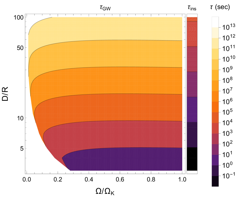
Figure 1: Instability growth time $\tau_{\mathrm{GW}}$ (in sec) as a function of the angular velocity $\Omega$ of the primary (normalized to the Kepler limit $\Omega_{\mathrm{K}}$; $x$-axis) and the orbital distance $D$ (normalized to the primary’s radius $R$; $y$-axis). The primary is a neutron star described by an $n=1$ polytropic equation of state, with $M=1.4\,M_{\odot}$ and $R=10\,\mathrm{km}$, orbited by an equal mass companion $(M^{\prime}=M)$. The inspiral time scale $\tau_{\mathrm{ins}}$ is also shown, as a function of the orbital distance, for comparison.

Assuming that the star is described by a polytrope with index $n=1$, we can now evaluate the instability time scale $\tau_{\mathrm{GW}}$ for the $l=2$ components of the equilibrium tide, the eigenfunctions of which can be obtained analytically (as shown in Appendix ). For a neutron star with $M=1.4\,M_{\odot}$ (where $M_{\odot}$ is the solar mass) and $R=10\,\mathrm{km}$ the instability growth time is given by

$$\tau_{\mathrm{GW}}=\Bigg{[}8.5\times 10^{-4}\left(\frac{D}{R}\right)^{9}F^{-1}(\Omega,D,M^{\prime})\\ +2.3\times 10^{-3}\left(\frac{D}{R}\right)^{6}F(\Omega,D,M^{\prime})\Bigg{]}\left(1+\frac{M^{\prime}}{M}\right)^{-5/2}.$$ (39)

In this model, $\nu_{\mathrm{K}}=\Omega_{\mathrm{K}}/2\pi\approx 2.2\,\mathrm{kHz}$. Equation 39 is plotted in Fig. 1 for $F(\Omega,D,M^{\prime})>0$ (i.e., where the instability is active) and $M^{\prime}=M$. For reasonable values of the mass ratio $M^{\prime}/M$, the time scale is not significantly affected.

III.2 Inspiral

The orbital motion of two stars generates GWs, gradually shrinking the binary’s orbit and eventually leading to its coalesence. For two point-like stars in a quasi-circular orbit the orbital separation changes due to quadrupole emission of GWs as (e.g., Maggiore2008,[0]Ref. Maggiore (2008))

$$\frac{\mathrm{d}D}{\mathrm{d}t}=-\frac{64G^{3}}{5c^{5}}\frac{MM^{\prime}(M+M^{\prime})}{D^{3}},$$ (40)

whereas the orbital phase $\Psi$ evolves according to

$$\frac{\mathrm{d}\Psi}{\mathrm{d}t}=\omega_{\mathrm{orb}}=\sqrt{\frac{G(M+M^{\prime})}{D^{3}}},$$ (41)

from which we also get

$$\frac{\mathrm{d}\omega_{\mathrm{orb}}}{\mathrm{d}t}=-\frac{3}{2}\frac{\dot{D}}{D}\omega_{\mathrm{orb}}.$$ (42)

The orbit is quasi-circular in the sense that the inspiral rate $|\dot{D}|/D$ is much smaller than $\omega_{\mathrm{orb}}$.

The energy of the tidal perturbation changes due to the orbital shrinking according to Eq. 15 which, evaluated for a certain harmonic of the equilibrium tide, gives

$$\left(\frac{\mathrm{d}E}{\mathrm{d}t}\right)_{\mathrm{ins}}=-(l+1)\frac{\dot{D}}{D}\frac{GM^{\prime}W_{l}^{m}}{D^{l+1}}\int_{0}^{R}\frac{\mathrm{d}\rho}{\mathrm{d}r}\frac{\delta\Phi+U}{g}r^{l+2}\mathrm{d}r$$ (43)

(note that the tidal potential $U$ and the perturbations are now functions not only of $r$, but also of $D(t)$, which will be henceforth implied). Using the relation between the mass multipole moments and the tidal Love number $k_{l}$ (e.g., YipLeung2017,[0]Ref. Yip and Leung (2017)), Eq. 43 can also be written as

$$\left(\frac{\mathrm{d}E}{\mathrm{d}t}\right)_{\mathrm{ins}}=-2k_{l}R^{2l+1}\frac{(2l+1)(l+1)}{4\pi G}\frac{\dot{D}}{D}\left(\frac{GM^{\prime}W_{l}^{m}}{D^{l+1}}\right)^{2}.$$ (44)

In a similar manner, the energy rate of the tidal perturbation due to GW emission is obtained from Eq. 16 as

$$\left(\frac{\mathrm{d}E}{\mathrm{d}t}\right)_{\mathrm{GW}}=\;(-1)^{l+1}N_{l}\left[\int_{0}^{R}\frac{\mathrm{d}\rho}{\mathrm{d}r}\frac{\delta\Phi+U}{g}r^{l+2}\mathrm{d}r\right]^{2}\\ \times\mathrm{Re}\left[(f^{*}-im\Omega)\left(f+\frac{\mathrm{d}}{\mathrm{d}t}\right)^{2l}f\right],$$ (45)

where $f(t)=-(l+1)\dot{D}/D-im\omega_{\mathrm{orb}}$. For $l\sim m\neq 0$ we have $|\mathrm{Re}(f)|\ll|\mathrm{Im}(f)|$. From Eq. 42 we also see that $\dot{\omega}_{\mathrm{orb}}\ll\omega_{\mathrm{orb}}^{2}$, which implies that derivatives of $\mathrm{Im}(f)$ can be neglected. Then, we recover Eqs. 34 and 35, albeit with a time dependence on $\omega_{\mathrm{orb}}$ and the perturbation variables. This can also be expressed in terms of the Love number as

$$\left(\frac{\mathrm{d}E}{\mathrm{d}t}\right)_{\mathrm{GW}}=-N_{l}(m\omega_{\mathrm{orb}})^{2l+2}\left(1-\frac{\Omega}{\omega_{\mathrm{orb}}}\right)\\ \times\left(2k_{l}R^{2l+1}\frac{2l+1}{4\pi G}\frac{GM^{\prime}W_{l}^{m}}{D^{l+1}}\right)^{2}.$$ (46)

The significance of the instability can be assessed by comparing the growth time $\tau_{\mathrm{GW}}$ to the inspiral time scale, given by

$$\tau_{\mathrm{ins}}=\frac{D}{|\dot{D}|}=\frac{5c^{5}}{64G^{3}}\frac{D^{4}}{MM^{\prime}(M+M^{\prime})}$$ (47)

which, for $M=1.4\,M_{\odot}$ and $R=10\,\mathrm{km}$, evaluates as

$$\tau_{\mathrm{ins}}=2.95\times 10^{-4}\left(\frac{D}{R}\right)^{4}\left[\frac{M^{\prime}}{M}\left(1+\frac{M^{\prime}}{M}\right)\right]^{-1}.$$ (48)

This is also plotted in Fig. 1, alongside the instability growth time. Both from Fig. 1 and from a direct comparison between Eqs. 39 and 48 it becomes evident that the inspiral time scale is shorter than the time required for the instability to develop for all values of $D$ and $\Omega$.

IV Implications

Using some simple arguments, we will present the implications of this instability of the equilibrium tide on the orbital and spin evolution, restricting ourselves to the quadrupole components $(l=2)$. The energy rate of the tidal perturbation, denoted below as $\dot{E}_{\mathrm{tide}}$, is given by Eqs. 44 and 46 and can be written as

$$\dot{E}_{\mathrm{tide}}=\epsilon\dot{E}_{\mathrm{tide}}^{(1)}+\epsilon^{2}\dot{E}_{\mathrm{tide}}^{(2)},$$ (49)

where

$$\epsilon=2k_{2}\left(1+\frac{M^{\prime}}{M}\right)\left(\frac{R}{D}\right)^{5}$$ (50)

and $\dot{E}_{\mathrm{tide}}^{(1)},\,\dot{E}_{\mathrm{tide}}^{(2)}$, which will be given below, contain the contributions of the inspiral and of GW emission to the energy rate of the tidal perturbation.

For a binary system in a quasi-circular orbit, where the tidal deformation of the primary (but not of the companion) is taken into account, the GW power emitted from the system is Chau (1976); Clark (1977)

$$\dot{E}_{\mathrm{GW}}=\dot{E}_{\mathrm{GW}}^{(0)}+\epsilon\dot{E}_{\mathrm{GW}}^{(1)}+\epsilon^{2}\dot{E}_{\mathrm{GW}}^{(2)},$$ (51)

where

$$\dot{E}_{\mathrm{GW}}^{(1)} =2\dot{E}_{\mathrm{GW}}^{(0)},$$ (52)

$$\dot{E}_{\mathrm{GW}}^{(2)} =\dot{E}_{\mathrm{GW}}^{(0)},$$ (53)

and

$$\dot{E}_{\mathrm{GW}}^{(0)}=-\frac{32G^{4}(MM^{\prime})^{2}(M+M^{\prime})}{5c^{5}D^{5}},$$ (54)

which is the point-mass limit Peters and Mathews (1963). Note that $\dot{E}_{\mathrm{GW}}$ is not to be confused with the contribution of GW emission to the energy rate of the tidal perturbation [Eqs. 16, 34, 45, and 46], which is here contained in $\dot{E}_{\mathrm{tide}}$ (see below).

Expanding the orbital energy losses in a similar way, we have

$$\dot{E}_{\mathrm{orb}}=\dot{E}_{\mathrm{orb}}^{(0)}+\epsilon\dot{E}_{\mathrm{orb}}^{(1)}+\epsilon^{2}\dot{E}_{\mathrm{orb}}^{(2)}.$$ (55)

At zeroth order in $\epsilon$, we simply get

$$\dot{E}_{\mathrm{orb}}^{(0)}=\dot{E}_{\mathrm{GW}}^{(0)},$$ (56)

from which we obtain the orbital decay in the point-mass limit, given by Eq. 40. Then, using this in Eq. 44, we get

$$\dot{E}_{\mathrm{tide}}^{(1)}=-\frac{6M^{\prime}}{M+M^{\prime}}\dot{E}_{\mathrm{GW}}^{(0)}.$$ (57)

Hence, the first-order correction to the orbital energy rate is

$$\dot{E}_{\mathrm{orb}}^{(1)}=\dot{E}_{\mathrm{GW}}^{(1)}-\dot{E}_{\mathrm{tide}}^{(1)}$$ (58)

or, replacing Eqs. 52 and 57,

$$\dot{E}_{\mathrm{orb}}^{(1)}=\left(2+\frac{6M^{\prime}}{M+M^{\prime}}\right)\dot{E}_{\mathrm{GW}}^{(0)}.$$ (59)

This can be used to calculate the first-order correction to the inspiral rate due to the tidal deformation of the primary. If $\dot{D}=\dot{D}^{(0)}+\epsilon\dot{D}^{(1)}$ (where $\dot{D}^{(0)}$ is the point-mass result), we find that

$$\dot{D}^{(1)}=\left(2+\frac{6M^{\prime}}{M+M^{\prime}}\right)\dot{D}^{(0)},$$ (60)

namely, the inspiral is accelerated, as expected Kochanek (1992).

At second order, both the inspiral and GW emission contribute to the tidal perturbation energy rate. The contribution of GW emission, obtained from Eq. 46, is

$$\dot{E}^{(2)}_{\mathrm{tide,\,GW}}=\left(1-\frac{\Omega}{\omega_{\mathrm{orb}}}\right)\dot{E}^{(0)}_{\mathrm{GW}}.$$ (61)

The contribution of the inspiral is found by replacing the first-order correction to the inspiral rate [Eq. 60] back to Eq. 44, which gives

$$\dot{E}^{(2)}_{\mathrm{tide,\,ins}}=-\frac{6M^{\prime}}{M+M^{\prime}}\left(2+\frac{6M^{\prime}}{M+M^{\prime}}\right)\dot{E}^{(0)}_{\mathrm{GW}}.$$ (62)

Thus, the second-order correction to the orbital energy rate is

$$\dot{E}_{\mathrm{orb}}^{(2)}=\dot{E}_{\mathrm{GW}}^{(2)}-\dot{E}_{\mathrm{tide}}^{(2)}-\dot{E}^{(2)}_{\mathrm{bg}},$$ (63)

where we also added possible changes in the energy of the background (unperturbed) star, $\dot{E}^{(2)}_{\mathrm{bg}}$. Replacing Eqs. 53, 61, and 62, we get

$$\dot{E}_{\mathrm{orb}}^{(2)}+\dot{E}^{(2)}_{\mathrm{bg}}=\left[\frac{\Omega}{\omega_{\mathrm{orb}}}+\frac{6M^{\prime}}{M+M^{\prime}}\left(2+\frac{6M^{\prime}}{M+M^{\prime}}\right)\right]\dot{E}^{(0)}_{\mathrm{GW}}.$$ (64)

In order to proceed with Eq. 64, we need to also consider the emission of angular momentum from the binary system. For GW emission from the tidal bulge, for which the second order term in Eq. 51 is responsible, angular momentum is emitted at a rate $\epsilon^{2}\dot{J}^{(2)}_{\mathrm{GW}}$, given by Thorne (1980); Chugunov (2019)

$$\dot{J}^{(2)}_{\mathrm{GW}}=\frac{\dot{E}^{(2)}_{\mathrm{GW}}}{\omega_{\mathrm{orb}}}.$$ (65)

Likewise, for the orbit we have

$$\dot{J}_{\mathrm{orb}}=\frac{\dot{E}_{\mathrm{orb}}}{\omega_{\mathrm{orb}}}.$$ (66)

The angular momentum rate associated with the tidal perturbation can be obtained by computing the torque applied on the star by the tidal force, as well as by the gravitational radiation reaction force, namely the force that accounts for GWs (see IpserLindblom1991,[0]Ref. Ipser and Lindblom (1991)). The total torque (along the $z$-axis) is given by Lai (1994)

$$T=\int\delta\rho\,\bm{e}_{z}\cdot\left(\bm{r}\times\bm{F}^{*}\right)\mathrm{d}^{3}\bm{r},$$ (67)

where $\bm{F}$ is the corresponding force (e.g., the tidal force is $\bm{F}=-\nabla U$). Evaluation of Eq. 67 shows that $\dot{J}^{(2)}_{\mathrm{tide,\,ins}}=0$, which is expected, since we are only considering the equilibrium tide where the tidal bulge is always aligned with the companion. In addition, we get

$$\dot{J}^{(2)}_{\mathrm{tide,\,GW}}=\frac{\dot{E}^{(2)}_{\mathrm{tide,\,GW}}}{\omega_{\mathrm{orb}}-\Omega}\;.$$ (68)

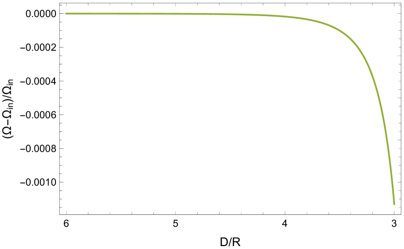
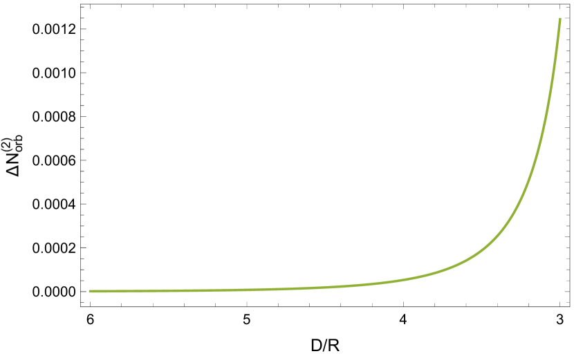
Figure 2: Change in the primary’s spin $\Omega$, relatively to its initial value $\Omega_{\mathrm{in}}$ (left), and second-order contribution to the number of orbital cycles $\Delta N_{\mathrm{orb}}^{(2)}$ (right), plotted against the orbital separation $D$ (normalized to the primary’s radius $R$). The primary is a neutron star described by an $n=1$ polytropic equation of state, with $M=1.4\,M_{\odot}$ and $R=10\,\mathrm{km}$, orbited by an equal mass companion $(M^{\prime}=M)$. The evolution is started at an orbital separation $D_{\mathrm{in}}=100\,R$ and the angular velocity of the primary is set to $\Omega_{\mathrm{in}}=0.3\,\Omega_{\mathrm{K}}$, where $\Omega_{\mathrm{K}}$ is the Kepler limit (for spherical stars). The binary merger is taken to occur at $3R$.

Hence, for the angular momentum emission from the system we have

$$\frac{\dot{E}^{(2)}_{\mathrm{GW}}}{\omega_{\mathrm{orb}}}=\frac{\dot{E}^{(2)}_{\mathrm{orb}}}{\omega_{\mathrm{orb}}}+\frac{\dot{E}^{(2)}_{\mathrm{tide,\,GW}}}{\omega_{\mathrm{orb}}-\Omega}+\frac{\dot{E}^{(2)}_{\mathrm{bg}}}{\Omega},$$ (69)

where we also replaced $\dot{E}^{(2)}_{\mathrm{bg}}=\Omega\dot{J}^{(2)}_{\mathrm{bg}}$. Using Eqs. 53 and 61, we finally obtain

$$\frac{\dot{E}^{(2)}_{\mathrm{orb}}}{\omega_{\mathrm{orb}}}=-\frac{\dot{E}^{(2)}_{\mathrm{bg}}}{\Omega},$$ (70)

which, replaced in Eq. 64, gives

$$\dot{E}^{(2)}_{\mathrm{orb}}=\frac{\displaystyle\frac{\Omega}{\omega_{\mathrm{orb}}}+\frac{6M^{\prime}}{M+M^{\prime}}\left(2+\frac{6M^{\prime}}{M+M^{\prime}}\right)}{\displaystyle 1-\frac{\Omega}{\omega_{\mathrm{orb}}}}\dot{E}^{(0)}_{\mathrm{GW}}$$ (71)

and

$$\dot{E}^{(2)}_{\mathrm{bg}}=\frac{\displaystyle\frac{\Omega}{\omega_{\mathrm{orb}}}+\frac{6M^{\prime}}{M+M^{\prime}}\left(2+\frac{6M^{\prime}}{M+M^{\prime}}\right)}{\displaystyle 1-\frac{\omega_{\mathrm{orb}}}{\Omega}}\dot{E}^{(0)}_{\mathrm{GW}}.$$ (72)

From Eqs. 71 and 72 we may now obtain the second-order correction to the inspiral rate $\epsilon^{2}\dot{D}^{(2)}$ and the background star’s spin derivative, respectively, as

$$\dot{D}^{(2)}=-\frac{\displaystyle F(\Omega,D,M^{\prime})+\left(1+\frac{M^{\prime}}{M}\right)^{1/2}+\mathcal{T}(M^{\prime})}{F(\Omega,D,M^{\prime})}\dot{D}^{(0)}$$ (73)

and

$$\frac{\dot{\Omega}}{\Omega_{\mathrm{K}}}=-\frac{\displaystyle F(\Omega,D,M^{\prime})+\left(1+\frac{M^{\prime}}{M}\right)^{1/2}+\mathcal{T}(M^{\prime})}{F^{2}(\Omega,D,M^{\prime})}\\ \times\frac{2\tilde{E}_{\mathrm{tide}}(\Omega,D,M^{\prime})}{\tau_{\mathrm{GW}}(\Omega,D,M^{\prime})}\left(\frac{D}{R}\right)^{3/2},$$ (74)

where

$$\mathcal{T}(M^{\prime})=12\frac{M^{\prime}}{M}\left(1+4\frac{M^{\prime}}{M}\right)\left(1+\frac{M^{\prime}}{M}\right)^{-3/2}$$ (75)

and

$$\tilde{E}_{\mathrm{tide}}=\frac{E_{\mathrm{tide}}}{I\Omega_{\mathrm{K}}^{2}},$$ (76)

with $E_{\mathrm{tide}}$ being the energy of the quadrupole components of the equilibrium tide [see Eq. 38] and $I$ being the background star’s moment of inertia. For a polytrope with $n=1$, $M=1.4\,M_{\odot}$ and $R=10\,\mathrm{km}$, we have

$$\tilde{E}_{\mathrm{tide}}=\,2.03\left(\frac{M^{\prime}}{M}\right)^{2}\left(\frac{D}{R}\right)^{-9}F^{2}(\Omega,D,M^{\prime})\\ +0.75\left(\frac{M^{\prime}}{M}\right)^{2}\left(\frac{D}{R}\right)^{-6},$$ (77)

whereas $\tau_{\mathrm{GW}}$ is given by Eq. 39.

Equation 73 predicts that, when the instability is active [$F(\Omega,D,M^{\prime})>0$], the inspiral is decelerated, which has also been shown to occur during the resonant excitation of CFS-unstable normal modes by the tide Ho and Lai (1999). On the other hand, according to Eq. 74, the spin of the (unperturbed) primary is decreasing when the instability occurs ($\tau_{\mathrm{GW}}>0$), in accordance with Chugunov2019,[0]Ref. Chugunov (2019), where the spin evolution equation is derived for unstable $r$-modes.

Solving the equations for $\dot{\Omega}$ and $\dot{D}=\dot{D}^{(0)}+\epsilon\dot{D}^{(1)}+\epsilon^{2}\dot{D}^{(2)}$, for the same model used above, we find that the change in the spin of the primary is negligible, as shown in Fig. 2. In the same figure, we also plot the second-order contribution to the number of orbital cycles, $\Delta N_{\mathrm{orb}}^{(2)}$, defined as Lai (1994)

$$N_{\mathrm{orb}}=\int\frac{\omega_{\mathrm{orb}}}{2\pi}\frac{\mathrm{d}D}{\dot{D}}=\int\frac{\omega_{\mathrm{orb}}}{2\pi}\frac{\mathrm{d}D}{\dot{D}^{(0)}+\epsilon\dot{D}^{(1)}}+\Delta N_{\mathrm{orb}}^{(2)},$$ (78)

with $N_{\mathrm{orb}}$ being the total number of orbits at second order. We see that the correction is positive, as expected from the discussion above, and accumulates very close to merger, as is the correction for the spin. However, this too is unimportant, at least for the parameters and the model considered here.

V Summary and discussion

We have shown that the equilibrium tide, namely the instantaneous hydrostatic response of a star to the tidal field of its companion, is unstable to the emission of gravitational radiation if the spin of the star exceeds the orbital angular velocity of the companion [Eqs. 35 and 36]. When this condition is fulfilled, the tidal perturbation, which is always prograde in the inertial frame, becomes retrograde in the frame rotating with the star. Then, the emission of GWs from the tidal bulge tends to increase the energy of the tidal perturbation on a secular time scale. This mechanism shares the same principles with the classic Chandrasekhar-Friedman-Schutz (CFS) instability for normal modes in rotating stars.

The instability growth time was calculated for a neutron star with $M=1.4\,M_{\odot}$ and $R=10\,\mathrm{km}$, described by a polytropic equation of state with a polytropic index $n=1$ [Eq. 39]. For this model, the eigenfunctions of the equilibrium tide can be derived analytically. As seen in Fig. 1, the instability is active in a very large part of the parameter space and the growth time varies by many orders of magnitude throughout the inspiral, depending mainly on the orbital separation and less on the spin of the star. Even though it can become as low as a few seconds very close to coalesence, the instability growth is always slower than the inspiral—at least for the chosen model.

Finally, the implications of the instability for orbital and spin evolution are explored, making use of some basic energy arguments. The corrections to the inspiral rate due to the tidal deformation and the emission of GWs from the tide are found [Eqs. 60 and 73], along with the change in the stellar spin [Eq. 74]. It is demonstrated that, when the instability is active, the emission of GWs from the tide slows down the inspiral, which has also been shown to be a consequence of the resonant excitation of CFS-unstable normal modes by the tide Ho and Lai (1999). Meanwhile, the angular velocity of the star decreases, evolving in a similar fashion as when under the influence of the classic CFS instability of normal modes Chugunov (2019). In Fig. 2 it is shown that, for the same model used above, the effects of the instability on orbital and spin evolution start becoming relevant—but still negligible—only very close to merger.

It should be noted that the rotation rates required for the instability to develop are unlikely to occur during the last stages of the binary evolution. However, near coalesence, the inspiral rate becomes too fast (plunge phase) for the quasi-cicrular orbit approximation to be accurate. Moreover, at this stage, the equilibrium tide approximation may also not be valid. If the tidal frequency is larger than the frequency of convective motions in the star (Brunt-Väisälä frequency), then the star responds effectively like a barotrope, in which case the equilibrium tide approximation fails Terquem et al. (1998); Goodman and Dickson (1998); Ogilvie (2014).

Furthermore, an important element which, for simplicity, has been neglected here is viscosity. Even though it makes the orbital evolution more dynamical, by introducing a lag between the orbital motion of the companion and the primary’s response, it has been shown not to significantly affect the orbital and spin evolution Kochanek (1992); Bildsten and Cutler (1992). Nevertheless, it is expected to supress the instability and shrink the parameter space where it is active, as in the case of CFS-unstable modes Ipser and Lindblom (1991).

From the above, it seems that the instability is purely of conceptual interest. Even so, there are some cases which might be worth considering in the future, like neutron stars described by stiffer equations of state, corresponding to larger deformabilities Hinderer (2008), or systems in which the neutron star has a much more massive companion.

*

APPENDIX Equilibrium tide in an $\bm{n=1}$ polytrope

The primary is described by a polytropic equation of state with polytropic index $n=1$, namely $p=K\rho^{2}$, where $K$ is the polytropic constant. For a star with mass $M$ and radius $R$, the Lane-Emden equations (e.g., see ShapiroTeukolsky1983,[0]Ref. Shapiro and Teukolsky (1983)) give

$$K=\frac{2GR^{2}}{\pi},$$ (79)

$$\rho_{c}=\frac{\pi M}{4R^{3}},$$ (80)

$$\rho=\rho_{c}\frac{\sin(\alpha r)}{\alpha r},$$ (81)

$$g=\frac{4\pi G\rho_{c}}{\alpha^{3}r^{2}}\left[\sin(\alpha r)-\alpha r\cos(\alpha r)\right],$$ (82)

where $\alpha=\pi/R$.

Replacing in Eq. 26 and combining with Eq. 4 we get

$$\frac{\mathrm{d}}{\mathrm{d}r}\left[r^{2}\frac{\mathrm{d}(\delta\Phi+U)}{\mathrm{d}r}\right]+\left[(\alpha r)^{2}-l(l+1)\right](\delta\Phi+U)=0$$ (83)

(the tidal potential $U$ and the perturbations include only their radial dependence), the solutions to which are the spherical Bessel functions $j_{l}(\alpha r)$ and $y_{l}(\alpha r)$ (e.g., AbramowitzStegun1972,[0]Ref. Abramowitz and Stegun (1972)). Retaining the solution that is regular at the origin and matching at the surface with the external solution for $\delta\Phi$, we obtain

$$\delta\Phi=\left\{\begin{array}[]{lr}\displaystyle\left[\frac{2l+1}{\pi j_{l-1}(\pi)}j_{l}(\alpha r)-\left(\frac{r}{R}\right)^{l}\right]U(R),&r\leq R,\\[20.00003pt] \displaystyle\frac{j_{l+1}(\pi)}{j_{l-1}(\pi)}\left(\frac{R}{r}\right)^{l+1}U(R),&r>R,\end{array}\right.$$ (84)

with $j_{l}$ given by

$$j_{l}(z)=z^{l}\left(-\frac{1}{z}\frac{\mathrm{d}}{\mathrm{d}z}\right)^{l}\frac{\sin z}{z}.$$ (85)

The equations above, together with Eq. 24 for the tidal potential, can now be used to obtain the eigenfunctions of the equilibrium tide, as presented in Sec. II.3.

References

- Kochanek (1992) C. S. Kochanek, “Coalescing binary neutron stars,” Astrophys. J. 398, 234–247 (1992).
- Bildsten and Cutler (1992) L. Bildsten and C. Cutler, “Tidal interactions of inspiraling compact binaries,” Astrophys. J. 400, 175–180 (1992).
- Hinderer (2008) T. Hinderer, “Tidal Love Numbers of Neutron Stars,” Astrophys. J. 677, 1216–1220 (2008), arXiv:0711.2420 .
- Flanagan and Hinderer (2008) É. É. Flanagan and T. Hinderer, “Constraining neutron-star tidal Love numbers with gravitational-wave detectors,” Phys. Rev. D 77, 021502 (2008), arXiv:0709.1915 .
- Abbott et al. (2017a) B. P. Abbott et al., “GW170817: Observation of Gravitational Waves from a Binary Neutron Star Inspiral,” Phys. Rev. Lett. 119, 161101 (2017a), 1710.05832 .
- Abbott et al. (2018) B. P. Abbott et al., “GW170817: Measurements of Neutron Star Radii and Equation of State,” Phys. Rev. Lett. 121, 161101 (2018), arXiv:1805.11581 [gr-qc] .
- Raithel et al. (2018) C. A. Raithel, F. Özel, and D. Psaltis, “Tidal Deformability from GW170817 as a Direct Probe of the Neutron Star Radius,” Astrophys. J. 857, L23 (2018), arXiv:1803.07687 [astro-ph.HE] .
- Radice et al. (2018) D. Radice, A. Perego, F. Zappa, and S. Bernuzzi, “GW170817: Joint Constraint on the Neutron Star Equation of State from Multimessenger Observations,” Astrophys. J. 852, L29 (2018), arXiv:1711.03647 [astro-ph.HE] .
- De et al. (2018) S. De, D. Finstad, J. M. Lattimer, D. A. Brown, E. Berger, and C. M. Biwer, “Tidal Deformabilities and Radii of Neutron Stars from the Observation of GW170817,” Phys. Rev. Lett. 121, 091102 (2018), arXiv:1804.08583 [astro-ph.HE] .
- Chandrasekhar (1970) S. Chandrasekhar, “Solutions of Two Problems in the Theory of Gravitational Radiation,” Phys. Rev. Lett. 24, 611–615 (1970).
- Friedman and Schutz (1978a) J. L. Friedman and B. F. Schutz, “Lagrangian perturbation theory of nonrelativistic fluids,” Astrophys. J. 221, 937–957 (1978a).
- Friedman and Schutz (1978b) J. L. Friedman and B. F. Schutz, “Secular instability of rotating Newtonian stars,” Astrophys. J. 222, 281–296 (1978b).
- Andersson (2003) N. Andersson, “TOPICAL REVIEW: Gravitational waves from instabilities in relativistic stars,” Classical Quantum Gravity 20, 105 (2003), astro-ph/0211057 .
- Pnigouras (2018) P. Pnigouras, Saturation of the -mode Instability in Neutron Stars, Springer Theses (Springer International Publishing, Cham, Switzerland, 2018).
- Papaloizou and Pringle (1978) J. Papaloizou and J. E. Pringle, “Non-radial oscillations of rotating stars and their relevance to the short-period oscillations of cataclysmic variables,” Mon. Not. R. Astron. Soc. 182, 423–442 (1978).
- Andersson (1998) N. Andersson, “A New Class of Unstable Modes of Rotating Relativistic Stars,” Astrophys. J. 502, 708–713 (1998), gr-qc/9706075 .
- Friedman and Morsink (1998) J. L. Friedman and S. M. Morsink, “Axial Instability of Rotating Relativistic Stars,” Astrophys. J. 502, 714–720 (1998), gr-qc/9706073 .
- Lai and Shapiro (1995) D. Lai and S. L. Shapiro, “Gravitational radiation from rapidly rotating nascent neutron stars,” Astrophys. J. 442, 259–272 (1995), astro-ph/9408053 .
- Owen et al. (1998) B. J. Owen, L. Lindblom, C. Cutler, B. F. Schutz, A. Vecchio, and N. Andersson, “Gravitational waves from hot young rapidly rotating neutron stars,” Phys. Rev. D 58, 084020 (1998), gr-qc/9804044 .
- Doneva et al. (2013) D. D. Doneva, E. Gaertig, K. D. Kokkotas, and C. Krüger, “Gravitational wave asteroseismology of fast rotating neutron stars with realistic equations of state,” Phys. Rev. D 88, 044052 (2013), arXiv:1305.7197 [astro-ph.SR] .
- Alford and Schwenzer (2014) M. G. Alford and K. Schwenzer, “What the Timing of Millisecond Pulsars Can Teach us about Their Interior,” Phys. Rev. Lett. 113, 251102 (2014), arXiv:1310.3524 [astro-ph.HE] .
- Doneva et al. (2015) D. D. Doneva, K. D. Kokkotas, and P. Pnigouras, “Gravitational wave afterglow in binary neutron star mergers,” Phys. Rev. D 92, 104040 (2015), arXiv:1510.00673 [gr-qc] .
- Levin (1999) Y. Levin, “Runaway Heating by R-Modes of Neutron Stars in Low-Mass X-Ray Binaries,” Astrophys. J. 517, 328–333 (1999), astro-ph/9810471 .
- Andersson et al. (2000) N. Andersson, D. I. Jones, K. D. Kokkotas, and N. Stergioulas, “R-Mode Runaway and Rapidly Rotating Neutron Stars,” Astrophys. J. 534, L75–L78 (2000), astro-ph/0002114 .
- Passamonti et al. (2013) A. Passamonti, E. Gaertig, K. D. Kokkotas, and D. Doneva, “Evolution of the f-mode instability in neutron stars and gravitational wave detectability,” Phys. Rev. D 87, 084010 (2013), arXiv:1209.5308 [astro-ph.SR] .
- Bondarescu et al. (2007) R. Bondarescu, S. A. Teukolsky, and I. Wasserman, “Spin evolution of accreting neutron stars: Nonlinear development of the r-mode instability,” Phys. Rev. D 76, 064019 (2007), arXiv:0704.0799 .
- Bondarescu et al. (2009) R. Bondarescu, S. A. Teukolsky, and I. Wasserman, “Spinning down newborn neutron stars: Nonlinear development of the r-mode instability,” Phys. Rev. D 79, 104003 (2009), arXiv:0809.3448 .
- Friedman (1983) J. L. Friedman, “Upper limit on the frequency of pulsars,” Phys. Rev. Lett. 51, 11–14 (1983).
- Andersson et al. (1999a) N. Andersson, K. Kokkotas, and B. F. Schutz, “Gravitational Radiation Limit on the Spin of Young Neutron Stars,” Astrophys. J. 510, 846–853 (1999a), astro-ph/9805225 .
- Andersson et al. (1999b) N. Andersson, K. D. Kokkotas, and N. Stergioulas, “On the Relevance of the R-Mode Instability for Accreting Neutron Stars and White Dwarfs,” Astrophys. J. 516, 307–314 (1999b), astro-ph/9806089 .
- Abbott et al. (2017b) B. P. Abbott et al., “Search for Post-merger Gravitational Waves from the Remnant of the Binary Neutron Star Merger GW170817,” Astrophys. J. 851, L16 (2017b), arXiv:1710.09320 [astro-ph.HE] .
- Abbott et al. (2019a) B. P. Abbott et al., “Search for Gravitational Waves from a Long-lived Remnant of the Binary Neutron Star Merger GW170817,” Astrophys. J. 875, 160 (2019a), arXiv:1810.02581 [gr-qc] .
- Abbott et al. (2019b) B. P. Abbott et al., “Searches for Continuous Gravitational Waves from 15 Supernova Remnants and Fomalhaut b with Advanced LIGO,” Astrophys. J. 875, 122 (2019b), arXiv:1812.11656 [gr-qc] .
- Abbott et al. (2019c) B. P. Abbott et al., “All-sky search for long-duration gravitational-wave transients in the second Advanced LIGO observing run,” Phys. Rev. D 99, 104033 (2019c), arXiv:1903.12015 [gr-qc] .
- Mashhoon (1973) B. Mashhoon, “Tidal Gravitational Radiation,” Astrophys. J. 185, 83–86 (1973).
- Mashhoon (1975) B. Mashhoon, “On tidal phenomena in a strong gravitational field,” Astrophys. J. 197, 705–716 (1975).
- Mashhoon (1977) B. Mashhoon, “Tidal radiation,” Astrophys. J. 216, 591–609 (1977).
- Turner (1977) M. Turner, “Tidal generation of gravitational waves from orbiting Newtonian stars. I - General formalism,” Astrophys. J. 216, 914–929 (1977).
- Will (1983) C. M. Will, “Tidal gravitational radiation from homogeneous stars,” Astrophys. J. 274, 858–874 (1983).
- Ho and Lai (1999) W. C. G. Ho and D. Lai, “Resonant tidal excitations of rotating neutron stars in coalescing binaries,” Mon. Not. R. Astron. Soc. 308, 153–166 (1999), astro-ph/9812116 .
- Reisenegger and Goldreich (1992) A. Reisenegger and P. Goldreich, “A new class of g-modes in neutron stars,” Astrophys. J. 395, 240–249 (1992).
- Unno et al. (1989) W. Unno, Y. Osaki, H. Ando, H. Saio, and H. Shibahashi, Nonradial Oscillations of Stars, 2nd ed. (University of Tokyo Press, Tokyo, 1989).
- Krüger et al. (2015) C. J. Krüger, W. C. G. Ho, and N. Andersson, “Seismology of adolescent neutron stars: Accounting for thermal effects and crust elasticity,” Phys. Rev. D 92, 063009 (2015), arXiv:1402.5656 [gr-qc] .
- Schenk et al. (2001) A. K. Schenk, P. Arras, É. É. Flanagan, S. A. Teukolsky, and I. Wasserman, “Nonlinear mode coupling in rotating stars and the r-mode instability in neutron stars,” Phys. Rev. D 65, 024001 (2001), gr-qc/0101092 .
- Thorne (1969) K. S. Thorne, “Nonradial Pulsation of General-Relativistic Stellar Models. IV. The Weak-field Limit,” Astrophys. J. 158, 997 (1969).
- Ipser and Lindblom (1991) J. R. Ipser and L. Lindblom, “The oscillations of rapidly rotating Newtonian stellar models. II. Dissipative effects,” Astrophys. J. 373, 213–221 (1991).
- Thorne (1980) K. S. Thorne, “Multipole expansions of gravitational radiation,” Rev. Mod. Phys. 52, 299–340 (1980).
- Zahn (1966) J. P. Zahn, “Les marées dans une étoile double serrée,” Ann. Astrophys. 29, 313 (1966).
- Ogilvie (2014) G. I. Ogilvie, “Tidal Dissipation in Stars and Giant Planets,” Annu. Rev. Astron. Astrophys. 52, 171–210 (2014), arXiv:1406.2207 [astro-ph.SR] .
- Ogilvie and Lin (2004) G. I. Ogilvie and D. N. C. Lin, “Tidal Dissipation in Rotating Giant Planets,” Astrophys. J. 610, 477–509 (2004), astro-ph/0310218 .
- Press and Teukolsky (1977) W. H. Press and S. A. Teukolsky, “On formation of close binaries by two-body tidal capture,” Astrophys. J. 213, 183–192 (1977).
- Steinborn and Ruedenberg (1973) E. O. Steinborn and K. Ruedenberg, “Rotation and Translation of Regular and Irregular Solid Spherical Harmonics,” Adv. Quantum Chem. 7, 1–81 (1973).
- Shapiro and Teukolsky (1983) S. L. Shapiro and S. A. Teukolsky, Black holes, white dwarfs, and neutron stars: The physics of compact objects (John Wiley & Sons, New York, 1983).
- Maggiore (2008) Michele Maggiore, Gravitational Waves: Theory and Experiments, Vol. 1 (Oxford University Press, Oxford, England, 2008).
- Yip and Leung (2017) K. L. S. Yip and P. T. Leung, “Tidal Love numbers and moment-Love relations of polytropic stars,” Mon. Not. R. Astron. Soc. 472, 4965–4981 (2017), arXiv:1709.02469 [astro-ph.SR] .
- Chau (1976) W. Y. Chau, “Finite Size Effect in Gravitational Radiation from Very Close Binary Systems,” Astrophys. Lett. 17, 119 (1976).
- Clark (1977) J. P. A. Clark, “Limits on the Finite Size Effect in Gravitational Radiation,” Astrophys. Lett. 18, 73 (1977).
- Peters and Mathews (1963) P. C. Peters and J. Mathews, “Gravitational Radiation from Point Masses in a Keplerian Orbit,” Phys. Rev. 131, 435–440 (1963).
- Chugunov (2019) A. I. Chugunov, “Long-term evolution of CFS-unstable neutron stars and the role of differential rotation on short time-scales,” Mon. Not. R. Astron. Soc. 482, 3045–3057 (2019), arXiv:1810.10379 [astro-ph.HE] .
- Lai (1994) D. Lai, “Resonant Oscillations and Tidal Heating in Coalescing Binary Neutron Stars,” Mon. Not. R. Astron. Soc. 270, 611 (1994), astro-ph/9404062 .
- Terquem et al. (1998) C. Terquem, J. C. B. Papaloizou, R. P. Nelson, and D. N. C. Lin, “On the Tidal Interaction of a Solar-Type Star with an Orbiting Companion: Excitation of g-Mode Oscillation and Orbital Evolution,” Astrophys. J. 502, 788–801 (1998), astro-ph/9801280 .
- Goodman and Dickson (1998) J. Goodman and E. S. Dickson, “Dynamical Tide in Solar-Type Binaries,” Astrophys. J. 507, 938–944 (1998), astro-ph/9801289 .
- Abramowitz and Stegun (1972) M. Abramowitz and I. A. Stegun, Handbook of Mathematical Functions (Dover, New York, 1972).