The connection between merging double compact objects and the Ultraluminous X-ray Sources

Abstract

We explore the different formation channels of merging double compact objects (DCOs: BH-BH/BH-NS/NS-NS) that went through a ultraluminous X-ray phase (ULX: X-ray sources with apparent luminosity exceeding $10^{39}\rm{\ erg\ s^{-1}}$). There are many evolutionary scenarios which can naturally explain the formation of merging DCO systems: isolated binary evolution, dynamical evolution inside dense clusters and chemically homogeneous evolution of field binaries. It is not clear which scenario is responsible for the majority of LIGO/Virgo sources. Finding connections between ULXs and DCOs can potentially point to the origin of merging DCOs as more and more ULXs are discovered. We use the StarTrack population synthesis code to show how many ULXs will form merging DCOs in the framework of isolated binary evolution. Our merger rate calculation shows that in the local Universe typically $50\%$ of merging BH-BH progenitor binaries have evolved through a ULX phase. This indicates that ULXs can be used to study the origin of LIGO/Virgo sources. We have also estimated that the fraction of observed ULXs that will form merging DCOs in future varies between $5\%$ to $40\%$ depending on common envelope model and metallicity.

1 Introduction

Ultraluminous X-ray sources (ULXs) are off-nuclear point sources with apparent X-ray luminosity above $10^{39}\rm{\ erg\ s^{-1}}$ (see Feng & Soria 2011; Kaaret et al. 2017 for review). The Eddington luminosity of typical X-ray binaries (neutron star $\sim 10^{38}\rm{\ erg\ s^{-1}}$ and a black hole of $10\ M_{\odot}\sim 10^{39}\rm{\ erg\ s^{-1}}$) are below the observed luminosity of ULXs. ULXs were considered as potential candidates for intermediate-mass black holes ($10^{2}-10^{5}M_{\odot}$) accreting at the sub-Eddington rate (Colbert & Mushotzky, 1999; Lasota et al., 2011), but the discovery of pulsating ULXs (Bachetti et al., 2014; Fürst et al., 2016; Israel et al., 2017a, b; Fürst et al., 2017; Carpano et al., 2018) demonstrated that the high luminosity of ULXs can be achieved by super-critical accretion onto a stellar-origin compact accretor as predicted by King et al. (2001), and confirmed by King & Lasota (2016); King et al. (2017); King & Lasota (2019) who found that the ULX luminosity results from beamed, anisotropic emission as suggested by King et al. (2001) (see also Wiktorowicz et al., 2019). Optical and near infrared observations showed that a few ULXs contain massive super-giant donors (Liu et al., 2007; Motch et al., 2011, 2014; Heida et al., 2015, 2016). Population synthesis study of field stars suggests that most ULXs contain $5-11\ M_{\odot}$ main sequence (MS) donors for black hole (BH) accretors and $0.9-1.5\ M_{\odot}$ MS donors for neutron star (NS) accretors (Wiktorowicz et al., 2017). These donors indicate that many ULXs are high-mass X-ray binaries (Swartz et al., 2011; Mineo et al., 2012) where the companion fills its Roche lobe and so transfers mass on a thermal timescale (King et al., 2001) and potential progenitors of close double compact objects (DCOs: BH-BH, BH-NS, NS-NS) (Finke & Razzaque, 2017; Marchant et al., 2017). Klencki & Nelemans (2018) explored a scenario of mass transfer from a massive donor with mass $M>15\ M_{\odot}$ onto a BH accretor leading to a ULX phase and eventually forming a short period BH-BH system.

The first detection of gravitational waves (GW150914) from two merging BHs of masses around $\sim 30\ M_{\odot}$ was made by the advanced Laser Interferometer Gravitational-wave Observatory (aLIGO) (Abbott et al., 2016). A total of eleven DCO mergers have been detected jointly by aLIGO and aVirgo during the first and second observing runs, out of which ten are BH-BH mergers and one is a NS-NS merger (Abbott et al., 2019). Venumadhav et al. (2019) discovered six additional new BH-BH mergers in the publicly available data from the second observing run of aLIGO/aVirgo.

There are many evolutionary scenarios which can explain the origin of BH-BH mergers: classical isolated binary evolution in galactic fields (Tutukov & Yungelson, 1993; Belczynski et al., 2016a; Kruckow et al., 2018), dynamical evolution inside dense star clusters (Portegies Zwart et al., 2004; Rodriguez et al., 2016; Chatterjee et al., 2017; Askar et al., 2017; Banerjee, 2018) and chemically homogeneous evolution of field binaries (Mandel & de Mink, 2016; de Mink & Mandel, 2016; Marchant et al., 2016). Since we do not know yet which scenario operates for most of the BH-BH mergers, we want to find the potential progenitors of BH-BH mergers to constrain their origin. On the other hand, the connection between ULXs and merging DCOs (hereafter mDCO if their delay time is shorter than the Hubble age) can be used to constrain the various poorly understood physical processes in binary stellar evolution (efficiency of common envelope, mass transfer, natal kick distribution, etc.). In the classical binary evolution, most progenitors of mDCOs experience one or two mass transfer phases (Belczynski et al., 2016a). If the mass transfer rate is high enough it may lead to a ULX phase. We investigate a scenario in which some of the ULXs may possibly form mDCOs in the context of classical isolated binary evolution as proposed in earlier studies (Finke & Razzaque, 2017; Marchant et al., 2017; Klencki & Nelemans, 2018). Finke & Razzaque (2017) did an analytical study assuming that all BH-BH mergers evolved through a ULX phase, which is still under debate. Klencki & Nelemans (2018) explored a small range of parameter, and they only considered BH-ULXs with high mass donors. Our study spans a wide range of parameter space, including the most up-to-date prescriptions of binary stellar evolution. Dominik et al. (2012) and Belczynski et al. (2016a) have done extensive studies of mDCOs and predicted the current LIGO and Virgo merger rates, whereas Wiktorowicz et al. (2015, 2017, 2019) have already drawn various conclusions about the population of ULXs, companion types and visibility. In this study we focus on the ULX formation channels that will form mDCOs at the end.

We note that the Be phenomenon (Zorec & Briot, 1997; Negueruela, 1998) and formation of ULXs containing Be star donors are not modeled in our simulations. The formation of decretion discs around Be stars (Lee et al., 1991) and the exact origin of different type of outbursts in galactic and extra-galactic Be stars is not yet fully understood (Negueruela et al. (2001); Negueruela & Okazaki (2001), but see Martin et al. (2014), who suggest that this involves Kozai–Lidov cycles in which the inclination of the decretion disc periodically coincides with the orbital plane, producing a massive outburst). There are at least five possible candidates of Be ULXs known at the moment; these ULXs are binary systems with orbital periods between 10 days to 100 days that exhibit transient phases of X-ray emission (Trudolyubov et al., 2007; Trudolyubov, 2008; Townsend et al., 2017; Tsygankov et al., 2017; Weng et al., 2017; Carpano et al., 2018; Doroshenko et al., 2018; Vasilopoulos et al., 2018). The accretors in these systems are NSs. Among these system, the Be star masses are known only for two systems. NGC 300 ULX1 has a $15-25M_{\odot}$ donor (Binder et al., 2016) and SMC X-3 has a $3.5M_{\odot}$ donor (Townsend et al., 2017). The donor mass in NGC 300 ULX1 is high enough that under favorable conditions, either through common envelope (CE) evolution or a well-placed kick, the future evolution of this system may lead to the formation of merging NS-NS binary.

In section 2 we explain our simulation setup. Section 3 describes the accretion model onto compact accretors and orbital, spin parameters change due to binary interactions. In section 4 we incorporate geometrical beaming in our population synthesis calculations in the context of ULX luminosity. We invoked two different CE models which are described in section 5. Section 6 describes our results and in section 7 we present the conclusions.

2 Simulation

We used StarTrack (Belczynski et al., 2002, 2008a), a rapid binary and single star population synthesis code with major updates as described in Dominik et al. (2012) and Belczynski et al. (2017). The primary (most massive) zero age main sequence (ZAMS) mass $M_{\rm a}$ was drawn within range $5-150\ M_{\odot}$ from three broken power-law distribution with index $\alpha=-1.3$ for $0.08\ M_{\odot}<M_{\rm a}\leq 0.5\ M_{\odot}$, $\alpha=-2.2$ for $0.5\ M_{\odot}<M_{\rm a}\leq 1\ M_{\odot}$, and $\alpha=-2.7$ for $M_{\rm a}>1.0\ M_{\odot}$ (Kroupa et al., 1993). The secondary ZAMS mass $M_{\rm b}$ ($0.5-150\ M_{\odot}$) was determined by the uniform distribution of binary mass ratio $q_{1}=M_{\rm b}/M_{\rm a}$ within range [0.1,1.0] (Sana et al., 2013). The orbital period ($P$) and the eccentricity ($e$) was selected, respectively, from the distributions $f(\text{log }P/\text{d})\sim(\text{log }P/\rm d)^{-0.55}$ with log $P$/d in the range [0.15,5.5] and $f(e)\sim e^{-0.42}$ within the interval [0.0,0.9] (Sana et al., 2013).

In our simulation, the rest of the physical assumptions are same as in the model M10 in Belczynski et al. (2016b) except for the accretion mechanism onto a compact accretor which we explain in the next section. In particular, our simulation includes the rapid supernova model (Belczynski et al., 2012; Fryer et al., 2012) to estimate the mass of the final compact object after the supernova explosion. This model also includes the pair-instability and the pair-instability pulsation supernovae which operate for helium cores with masses $M_{\rm He}>60-65M_{\odot}$ and $M_{\rm He}>40-45M_{\odot}$, respectively (see Belczynski et al., 2016b, and references therein). The natal kick strength ($v_{\rm kick}$) during birth of a BH/NS was drawn from a Maxwellian distribution with $\sigma=265\ \rm{km\ s^{-1}}$ (Hobbs et al., 2005), but decreased by the fraction of ejected mass that falls back onto the compact object. The final kick velocity given to a BH/NS is $v_{\rm kick,fin}=v_{\rm kick}(1-f_{\rm fb})$, and $f_{\rm fb}$ is the fraction of ejected mass that falls back onto the compact object. We assumed that a BH formed via direct collapse does not receive a natal kick.

We simulated $2\times 10^{6}$ binary systems with 32 different metallicities ($Z$) from $Z=0.005Z_{\odot}$ to $Z=1.5Z_{\odot}$. The exact value of $Z_{\odot}$ is not settled (Vagnozzi et al., 2017); we adopted the value of $Z_{\odot}=0.02$. The binary fraction was chosen to be 50% for primary ZAMS mass below $10\ M_{\odot}$ and 100% above $10\ M_{\odot}$ (Duchêne & Kraus, 2013; Sana et al., 2013). The total simulated stellar mass at each metallicity is $M_{\rm sim}=4.4\times 10^{8}M_{\odot}$. Note that we have not used any specific star formation history in the context of the ULXs. In our simulation, all the stars are born at the same time. Our results give the total number of ULXs for a given metallicity that form at any time during the 10 Gyr evolution of an ensemble of stars with an initial total mass of $4.4\times 10^{8}M_{\odot}$.

The same simulation provides a specific number of DCOs for different metallicities. To calculate the cosmic merger rate density of these double compact objects as a function of redshift $z$, we need to use the star formation history SFR($z$) in the Universe and the metallcity evolution as a function of redshift Z($z$).

SFR($z$) we adopt from Madau & Dickinson (2014),

$$\text{SFR}(z)=0.015\frac{(1+z)^{2.7}}{1+\left(\frac{1+z}{2.9}\right)^{5.6}}\ M_{\odot}\rm{\ Mpc^{-3}\ yr^{-1}}.$$ (1)

We calculated the merger rates from $z=0$ to 15. At each given redshift, we chose a redshift bin with size $\Delta z=0.1$ to calculate the comoving volume $dV_{\rm c}(z)$,

$$dV_{\rm c}(z)=\frac{c}{H_{0}}\frac{D_{\rm c}^{2}}{E(z)}\Delta z$$ (2)

where $D_{c}$ is the comoving distance is given by,

$$D_{\rm c}=\frac{c}{H_{0}}\int_{0}^{z}\frac{dz^{\prime}}{E(z^{\prime})}$$ (3)

with $E(z)=\sqrt{\Omega_{\rm M}(1+z)^{3}+\Omega_{\rm K}(1+z)^{2}+\Omega_{\Lambda}}$. $\Omega_{\rm M}$, $\Omega_{\rm K}$ and $\Omega_{\Lambda}$ are the usual cosmological density–parameters. The total stellar mass at a given redshift was determined by multiplying the SFR($z$) with $dV_{\rm c}(z)$ and the corresponding time interval of $\Delta z$. Then the obtained total stellar mass was used to normalize the simulated stellar mass.

To include the contribution from different metallicities, at each redshift we used a log-normal distribution of metallicity around the average metallicity ($Z_{\rm avg}$), with a standard deviation of $\sigma=0.5$ dex (Dvorkin et al., 2015). The equation for average metallicity was taken from Madau & Dickinson (2014) with logarithmic of the average metallicity is increased by 0.5 dex to better fit the observational data (Vangioni et al., 2015)

$$\leavevmode\resizebox{469.75499pt}{}{ $\text{log}[\text{Z}_{\rm avg}(z)]=0.5+\text{log}\bigg{(}\frac{y(1-R)}{\rho_{\rm b}}\bigintss_{z}^{20}\frac{97.8\times 10^{10}\text{SFR}(z^{\prime})}{H_{0}E(z^{\prime})(1+z^{\prime})}dz^{\prime}\bigg{)}$},$$ (4)

where $y=0.019$, $R=0.27$, baryon density $\rho_{\rm b}=2.27\times 10^{11}\Omega_{\rm b}h_{0}^{2}\ M_{\odot}\rm{\ Mpc^{-3}}$. Throughout our study, we assumed flat cosmology with $h_{0}=0.7$, $\Omega_{\rm b}=0.045$, $\Omega_{\rm M}=0.3$, $\Omega_{\rm K}=0$, $\Omega_{\Lambda}=0.7$ and $H_{0}=70.0\rm{\ km\ s^{-1}Mpc^{-1}}$.

3 ACCRETION MODEL

3.1 Roche lobe overflow (RLOF) accretion/luminosity

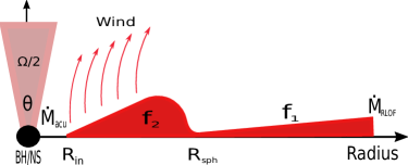
Figure 1: Schematic diagram of the super-critical accretion disk around a compact accretor. $R_{\rm in}$ and $R_{\rm sph}$ are the inner and the spherization radius of the accretion disk. $f_{1}$ and $f_{2}$ parameters determine the wind mass loss rate from the outer and the inner part (inside $R_{\rm sph}$) of the disk. $\dot{M}_{\rm RLOF}$ is the mass transfer rate from the donor star and $\dot{M}_{\rm acu}$ is the mass accumulation rate onto the compact accretor. $\theta$ and $\Omega$ are the opening angle and the total solid angle of the emitted beam, respectively.

In a close binary system when the matter is transferred from the donor star to the compact accretor an accretion disk is formed. We adopted the accretion disk model from Shakura & Sunyaev (1973). At low accretion rates (sub-critical) the disk does not produce strong outflows. At super-critical accretion rates, below the spherization radius the disk is dominated by radiation pressure, which leads to strong outflows. In super-critical accretion regime, the local disk luminosity is Eddington limited, most of the gas is blown away by radiation pressure and the accretion rate decreases linearly with radius (see Fig. 1).

This accretion model is used for both RLOF and wind mass accretion. First, we will discuss the RLOF accretion, the wind accretion is described in next section. During the Roche lobe overflow phase, $\dot{M}_{\rm RLOF}$ is the mass that has been transferred from donor star to the disk around compact accretor. Mass loss by the disk wind from the outer part of the disk down to the spherization radius ($R_{\rm sph}$) of the disk is taken care by a factor $f_{1}$. The mass accretion rate at $R_{\rm sph}$ is then

$$\dot{M}_{\rm 0,RLOF}=f_{1}\dot{M}_{\rm RLOF},$$ (5)

but in what follows we have assumed $f_{1}=1$ (no wind from the outer disk). Inside the spherization radius ($R_{\rm sph}$), the disk is dominated by radiation pressure which leads to strong wind.

One can calculate the spherization radius from

$$R_{\rm sph}=\frac{27}{4}\frac{\dot{M}_{\rm 0,RLOF}}{\dot{M}_{\rm Edd}}R_{\rm S},$$ (6)

where $R_{\rm S}=2GM/c^{2}$ is the Schwarzschild radius of the accreting compact object.

The Eddington accretion rate ($\dot{M}_{\rm Edd}$) is given by

$$\dot{M}_{\rm Edd}\equiv\frac{L_{\rm Edd}}{0.1c^{2}}=4.43\times 10^{-8}(1+X)^{-1}\frac{M}{M_{\odot}}\ M_{\odot}\rm{\ yr^{-1}}$$ (7)

where $L_{\rm Edd}=4\pi cGM/\kappa$, with $\kappa=\sigma_{\rm T}(1+X)/2m_{\rm p}$. $\sigma_{\rm T}$ is Thomson scattering cross-section for an electron, $m_{\rm p}$ is the mass of a proton, $G$ is gravitational constant and $c$ is the speed of light. The efficiency of gravitational energy release is $\sim$ 0.1. We take the hydrogen mass fraction in donor envelope $X$ to be 0.7 for H-rich donor stars and 0 for H-deficient donor stars. The radius of a NS ($R_{\rm NS}$) can be derived from

$$R_{\rm NS}=47.44-64.77\frac{M}{M_{\odot}}+39.12\left(\frac{M}{M_{\odot}}\right)^{2}-7.90\left(\frac{M}{M_{\odot}}\right)^{3}\text{ km}$$ (8)

where $M$ is mass of a NS. The above formula was obtained by using a polynomial fit to the data points of model number BSk20 from Fortin et al. (2016). The fit has been applied in the mass range from $1.39\ M_{\odot}$ to $2.17\ M_{\odot}$. We have considered the radius to be constant: $R_{\rm NS}=10.37$ km for NS with masses above $2.17\ M_{\odot}$ and $R_{\rm NS}=11.77$ km for NS with masses below 1.39 $M_{\odot}$.

For the case of the non-magnetized neutron star, the inner accretion disk radius, we assumed to be:

$$R_{\rm accNS}=R_{\rm NS},$$ (9)

and for an accreting black hole:

$$R_{\rm accBH}=R_{\rm ISCO},$$ (10)

where $R_{\rm ISCO}$ is innermost stable circular orbit radius:

$$R_{\rm ISCO}=\frac{GM}{c^{2}}\left\{3+Z_{2}-[(3-Z_{1})(3+Z_{1}+2Z_{2})]^{\frac{1}{2}}\right\},$$ (11)

where

$$Z_{2} =(3a_{\rm spin}^{2}+Z_{1}^{2})^{\frac{1}{2}}$$ (12)

$$Z_{1} =1+(1-a_{\rm spin}^{2})^{\frac{1}{3}}[(1+a_{\rm spin})^{\frac{1}{3}}+(1-a_{\rm spin})^{\frac{1}{3}}]$$ (13)

where

$$a_{\rm spin}=\frac{Jc}{GM^{2}}$$ (14)

is the BH dimensionless spin magnitude, $M$ and $J$ are respectively the mass and the spin angular momentum of a BH. For $a_{\rm spin}=0$, $R_{\rm ISCO}=3R_{\rm S}$. $R_{\rm ISCO}$ increases for retrograde motion of an orbit with respect to the BH spin, whereas in prograde motion, it comes closer to the horizon. We assumed the prograde rotation of the disk around the BH.

The mass accumulation rate $\dot{M}_{\rm acu,RLOF}$ onto the compact accretor is

$$\dot{M}_{\rm acu,RLOF}=f_{2}\dot{M}_{\rm 0,RLOF}=f_{1}f_{2}\dot{M}_{\rm RLOF},$$ (15)

where (1-$f_{2}$) denotes wind mass loss from the inner part of a disk (inside $R_{\rm sph}$). This part of the disk is assumed to be in radiation dominated regime and effectively losing mass in disk winds.

• If the mass transfer rate $\dot{M}_{\rm 0,RLOF}$ is larger than the Eddington mass accretion rate $\dot{M}_{\rm Edd}$ then

  $$f_{2}=\frac{R_{\rm acc}}{R_{\rm sph}}$$ (16)

  and equation 15 simplifies to

  $$\dot{M}_{\rm acu,RLOF}=\frac{4R_{\rm acc}}{27R_{\rm S}}\dot{M}_{\rm Edd}.$$ (17)

  The spherically isotropic luminosity of an accreting compact object is then given by (Shakura & Sunyaev, 1973)

  $$L_{\rm x,iso}=L_{\rm Edd}\bigg{[}1+\ln{\bigg{(}\frac{\dot{M}_{\rm 0,RLOF}}{\dot{M}_{\rm Edd}}\bigg{)}}\bigg{]}.$$ (18)

• If the mass accretion rate $\dot{M}_{\rm 0,RLOF}$ is lower then the Eddington accretion rate then

  $$f_{2}=1$$ (19)

  and

  $$L_{\rm x,iso}=\eta\dot{M}_{\rm 0,RLOF}c^{2}$$ (20)

  where $\eta$ is efficiency of gravitational energy release. For NS, (Shakura & Sunyaev, 1973)

  $$\eta_{\rm NS}=\frac{GM}{c^{2}R_{\rm accNS}}$$ (21)

  $\eta_{\rm NS}$ varies from 17% for 1.4 $M_{\odot}$ NS to 28% for 2.1 $M_{\odot}$ NS. For BH,

  $$\eta_{\rm BH}=1-E(R_{\rm ISCO})$$ (22)

  $$E(R)=\frac{R^{2}-2\frac{GM}{c^{2}}R+a_{\rm spin}\frac{GM}{c^{2}}\bigg{(}\frac{GM}{c^{2}}R\bigg{)}^{1/2}}{R\bigg{(}R^{2}-3\frac{GM}{c^{2}}R+2a_{\rm spin}\frac{GM}{c^{2}}\bigg{(}\frac{GM}{c^{2}}R\bigg{)}^{1/2}\bigg{)}^{1/2}}$$ (23)

  where $E(R=R_{\rm ISCO})$ is specific keplerian energy at ISCO radius. $\eta_{\rm BH}$ varies from 6% for $a_{\rm spin}=0$ to 42% for $a_{\rm spin}=1$.

The mass ejection rate $\dot{M}_{\rm eje,RLOF}$ from a disk around a compact accretor is determined by

$$\dot{M}_{\rm eje,RLOF}=\dot{M}_{\rm RLOF}-\dot{M}_{\rm acu,RLOF}.$$ (24)

3.2 Wind accretion/luminosity

For the description of wind accretion we have used the Bondi & Hoyle (1944) accretion mechanism. The compact accretor captures a fraction of the mass lost from the donor by stellar wind

$$\dot{M}_{\rm acc,WIND}=f_{\rm wind}\dot{M}_{\rm WIND},$$ (25)

where $f_{\rm wind}$ determines the mean accretion rate into the disk around compact accretor. The prescription for $f_{\rm wind}$ has been taken from Hurley et al. (2002). Here $\dot{M}_{\rm WIND}$ is wind mass loss rate from the donor star and $\dot{M}_{\rm acc,WIND}$ is wind mass accretion rate onto the disk around the compact accretor. $f_{\rm wind}$ is given by,

$$f_{\rm wind}=\frac{1}{\sqrt{1-e^{2}}}\bigg{(}\frac{GM_{\rm acc}}{v_{\rm wind}^{2}}\bigg{)}^{2}\frac{\alpha_{\rm wind}}{2a^{2}}\frac{1}{(1+v^{2})^{3/2}}$$ (26)

where $\alpha_{\rm wind}=1.5$, $v=v_{\rm orb}/v_{\rm wind}$ and

$$v_{\rm orb}=\sqrt{\frac{G(M_{\rm acc}+M_{\rm don})}{a}}.$$ (27)

The wind velocity is simply assumed to be the escape velocity at the donor surface with a factor $\sqrt{\beta_{\rm wind}}$,

$$v_{\rm wind}=\sqrt{\beta_{\rm wind}\frac{2GM_{\rm don}}{R_{\rm don}}}.$$ (28)

$\beta_{\rm wind}$ varies from 0.7 to 0.125 depending on the spectral type of the donor star. We treated the rest of the problem the same way as for the RLOF accretion which translates to

$$\dot{M}_{\rm acu,WIND}=f_{\rm wind}f_{1}f_{2}\dot{M}_{\rm WIND}$$ (29)

$$\dot{M}_{\rm eje,WIND}=\dot{M}_{\rm acc,WIND}-\dot{M}_{\rm acu,WIND}$$ (30)

$$\dot{M}_{\rm 0,WIND}=f_{1}f_{\rm wind}\dot{M}_{\rm WIND}$$ (31)

with $f_{1}$ and $f_{2}$ the same as in Section 3.1.

3.2.1 Orbital parameter change

We assumed a spherically symmetric wind mass-loss from the donor which carries away the angular momentum from the binary system (Jeans-mode mass loss). This leads to orbital expansion. The corresponding change in orbit due to the angular momentum loss is calculated from

$$a(M_{\rm acc}+M_{\rm don})=\text{constant},$$ (33)

where only $M_{\rm don}$ changes by $\dot{M}_{\rm don}=(1-f_{\rm wind})\dot{M}_{\rm WIND}$ (Belczynski et al., 2008a). The accumulation of mass on the compact accretor is very low compared to the wind mass-loss from the donor making and is not significantly affecting the orbital separation. In the case of super-critical accretion, the binary orbital separation further increases due to the wind mass loss from the inner part of the disk (inside $R_{\rm sph}$). We assume the matter ejected by the disk wind carries away the specific angular momentum of the compact accretor. The angular momentum loss specific to the accreting compact object can be obtained from

$$\frac{dJ}{dt} =R_{\rm com}^{2}\Omega_{\rm orb}\dot{M}_{\rm eje,RLOF/WIND}$$ (34)

$$R_{\rm com} =a\frac{M_{\rm don}}{M_{\rm acc}+M_{\rm don}}$$ (35)

$$\Omega_{\rm orb} =\sqrt{G(M_{\rm acc}+M_{\rm don})}a^{-1.5},$$ (36)

where $R_{\rm com}$ is the distance between the accretor and the binary’s centre of mass.

3.2.2 Compact object spin change

The spin of the BH accretor increases due to accretion which changes the ISCO radius. The angular momentum $l$ and energy $E$ of the accumulated mass $M_{\rm acu}$ can be calculated from equation (23) and from equation (3) in Belczynski et al. (2008b). Final mass and spin angular momentum of the BH accretor will be

$$M_{\rm f} =M_{\rm i}+\frac{E}{c^{2}}$$ (37)

$$J_{\rm f} =J_{\rm i}+l$$ (38)

where the initial spin angular momentum is calculated from $J_{\rm i}=a_{\rm spin,i}M_{\rm i}^{2}G/c$ and the final spin will be $a_{\rm spin,f}=J_{\rm f}c/GM_{\rm f}^{2}$.

4 BEAMING MODEL

At high mass accretion rate luminosity could be collimated through small cones then the observed luminosity will be much higher than $L_{\rm x,iso}$ (spherically isotropic) this phenomenon is called beaming (King et al., 2001). The beaming factor $b$ has been defined as $b=\Omega/4\pi$ (King, 2009). If we consider the emission through two conical sections, the total solid angle of emission $\Omega=4\pi[1-\cos(\theta/2)]$, here $\theta$ is the opening angle of the cone. The apparent luminosity is

$$L_{\rm x,beam}=\frac{L_{\rm x,iso}}{b}.$$ (39)

In our simulation, we identified the ULX when the apparent X-ray luminosity ($L_{\rm x,beam}$) of the accreting compact object exceeds $10^{39}$ erg s^-1 at some point during its lifetime. From comparison with observations King (2009) obtained for the beaming parameter $b$

$$b=\begin{cases}\frac{73}{\dot{m}_{0}^{2}},&\dot{m}_{0}\geq 8.5\\ 1,&\dot{m}_{0}<8.5,\\ \end{cases}$$ (40)

where, since we assume $f_{1}=1$, $\dot{m}_{0}=\dot{M}_{\rm 0,RLOF}/\dot{M}_{\rm Edd}$ is mass accretion rate at $R_{\rm sph}$ in Eddington accretion-rate unit. In Wiktorowicz et al. (2017) the beaming was assumed to saturate at very high accretion rates; an assumption we are not using in the present paper (see Wiktorowicz et al., 2019).

5 Hertzsprung gap donors — submodel A and B

In the scheme of close binary evolution probably the most crucial point is the CE phase. If the mass transfer is dynamically unstable, it will lead to a CE phase (see Ivanova et al. 2013 for review). The CE phase brings the stars closer by transferring the orbital energy to the envelope, which is necessary to explain the observed population of low mass X-ray binaries (Liu et al., 2007, see, however, Wiktorowicz et al. (2014)) and the mDCOs (Dominik et al., 2012). During the CE phase, the binary system goes through spiral–in phase, which, if the envelope is not ejected, will lead to a premature merger. If the donor star does not have a well developed core, then the orbital energy is transferred to the entire star, which makes it hard to eject the envelope. Stars on the MS branch do not have a clear core-envelope boundary. Similarly stars on the Hertzsprung gap (HG) branch lack the clear entropy difference related to the core-envelope structure (Ivanova & Taam, 2004). We assume that a CE initiated by a MS donor always result to the merger. Further we extend our analysis for HG donors. In submodel A, we followed the standard energy balance prescription of the CE for HG donors, whereas in submodel B (more conservative approach), we assume the binary does not survive the CE initiated by HG donor. We note that systems such as Cyg X-2 have avoided the CE phase despite having large mass ratio during the onset of mass transfer phase $q\sim 2.6$ (King & Ritter, 1999). This type of system can be explained by recent study of Pavlovskii et al. (2017), who revisited the stability of mass transfer and showed that at some cases the mass transfer can be stable even at very high mass ratio. The study by Pavlovskii et al. (2017) was limited to very small range of metallicities (only at $0.1Z_{\odot}$ and $Z_{\odot}$). We have not yet included this type of mass transfer scheme in our current study, even if it might explain the nature of at least some ULXs (see, e.g. King & Lasota, 2019). In future, we will include this type of mass transfer scheme and stellar rotation in StarTrack using MESA model.

6 Results

6.1 Metallicity effect on the ULX population

Metallicity plays a crucial role in the binary stellar evolution. The formation number of ULXs can be very different at different metallicities. The numbers presented here are of ULXs formed out of the same stellar mass ($M_{\rm sim}=4.4\times 10^{8}\ M_{\odot}$) at different metallicities. We found that ULXs can be powered by both RLOF and wind mass transfer. Typically, RLOF ULXs are brighter than wind-fed ULXs. In general, more than $\sim 50\%$ of the entire RLOF ULX population have apparent luminosities larger than $10^{40}\rm{\ erg\ s^{-1}}$. In contrast, no more than $\sim 10\%$ of all wind accreting ULXs have apparent luminosities larger than $10^{40}\rm{\ erg\ s^{-1}}$.

The upper panel of Fig. 2 shows the number of RLOF BH- and NS-ULXs formed at different metallicities. For comparison we also show the total number of NS and BH binary formed.

6.1.1 BH-ULXs

The number of BH-ULXs remains almost constant at low metallicity ($0.005Z_{\odot}\leq Z<0.2Z_{\odot}$) but decreases at higher values (dotted blue lines). The mass–loss due to stellar winds plays a major role only for rather high metallicity which explains the relative insensitivity of the number of ULXs formed at low metallicity values.

At higher metallicity, there are three main factors which contribute to the decreasing numbers of BH-ULXs. They are: the wind mass loss, the stability properties of the mass-transfer and the natal kick.

(1) The wind mass loss rate from a metal rich star is very high as compared to a metal-poor star (Vink et al., 2001; Vink & de Koter, 2005). Increasing wind mass-loss with metallicity puts the binary components further apart, which makes it hard to achieve the RLOF.

(2) The thermal timescale mass transfer via RLOF is allowed only when the-donor-to-accretor mass ratio at the onset of the RLOF is less then the critical value ($q_{\rm crit}$). If the mass ratio is $\geq q_{\rm crit}$, then mass transfer proceeds on dynamical timescale which leads to a CE phase. For rapid thermal timescale mass transfer we use a diagnostic diagram to determine $q_{\rm crit}$ which varies between $1.2-2.0$ depending on the type of donor (Belczynski et al., 2008a, Section 5.2). Stars with a radiative envelope, but with a deep convective layer are subject to delayed dynamical instability. King & Begelman (1999) suggested that donor with radiative envelope does not lead to the CE phase. However, once donor convective layer is exposed it can evolve into a delayed CE phase. For delayed dynamical instability we used $q_{\rm crit}=3.0$ for H-rich donors, $q_{\rm crit}=1.7$ for He main sequence donors, $q_{\rm crit}=3.5$ for evolved He donors (Belczynski et al., 2008a). Blue solid line in Fig. 3 shows the average BH mass decreases with increasing metallicity (Belczynski et al., 2010a). As metallicity increases the limit on the donor mass for stable mass transfer becomes narrower, which allows only a fraction of binary systems to go through the stable mass-transfer phase, as a result the number of RLOF BH ULXs diminishes.

(3) The overall number of binary systems with BH accretors decreases as metallicity increases, which in turn lowers the number of RLOF BH ULXs (see blue dash/solid line in Fig. 2). The overall number of BH binary systems decreases mainly due to formation of low mass BHs. Low mass BHs receive natal kick during its formation, which can potentially disrupt the binary systems.

The bottom panel of Fig. 2 shows the number of wind BH-ULXs, which remains nearly constant in all tested metallicities (dotted blue lines). This can be understood comparing it to the total number of binary systems formed with BH accretors. The number of such systems decreases with increasing metallicity, as explained in (3) above. The wind mass-loss rate increases with metallicity (Vink et al., 2001; Vink & de Koter, 2005). Due to low wind mass-loss rate at low metallicity, only a fraction of binary systems have a mass-loss large enough to power a ULX. At high metallicity, although the number of companion stars that can provide the required wind mass-loss rate is higher, the number of binary systems with BH accretors decreases. Consequently, the number of wind BH-ULXs remains roughly constant throughout metallicity.

6.1.2 NS-ULXs

The number of NS-ULXs does not depend much on metallicity (dashed red lines in Fig. 2). This is because, the donors mass in NS-ULXs are very low (Wiktorowicz et al., 2017, 2019). In our simulation, the average donor mass in both type of NS-ULXs are in between $1-2\ M_{\odot}$ (red and black lines in Fig. 3). For low mass donors both the wind mass loss rates and the mass transfer rates are independent of metallicity, so their evolution remains nearly unaffected by metallicity.

Most NS-ULXs reach ULX luminosities through beaming of emission. For a given mass transfer rate, NS will always have lower opening angle of emission than BH, which increases the apparent luminosity of NS-ULXs (King & Wijnands, 2006; King & Lasota, 2016; Wiktorowicz et al., 2019).

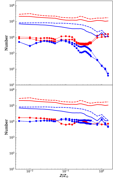
Figure 2: The total number of ULXs formed in our simulation for different metallicities (line–connected dots). For comparison we also show the total number of binary systems with NS and BH accretors (lines with no dots). Color red corresponds to accreting NS, color blue to accreting BH. Dashed lines correspond to submodel A, continuous lines to submodel B. Upper panel: ULX with RLOF mass transfer. Bottom Panel: ULX in wind mass transfer phase. For NS-ULXs submodels A and B overlap.

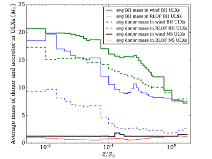
Figure 3: Average masses of donors and accretors for different ULX channels in submodel B ( results for submodel A are similar ). The average mass of the accretor and donor in both type of BH-ULXs decreases as metallicity increases. The average donor mass in NS-ULXs remains almost constant independent of metallicity ($\sim 1.25M_{\odot}$ for wind NS ULXs and $\sim 1.0M_{\odot}$ for RLOF NS ULXs).

6.2 Metallicity effect on the mDCOs population

The populations of mDCOs depend strongly on metallicity. Fig. 4 shows the formation number of mDCOs at different metallicities. These results are well known from the previous studies (Belczynski et al., 2010b; Dominik et al., 2012; Klencki et al., 2018). The number of BH-BH formation increases with decreasing metallicity. This is mainly because the BH mass increases as metallicity decreases (Belczynski et al., 2010a). Higher mass BHs receive little to no natal kick during their formation, which leads to the survival of large number of binary systems. The formation efficiency of BH-NS systems does not increases the same way as BH-BH does with decreasing metallicity. This is because most of the binary systems are disrupted during the formation of NSs. The next interesting point to note is that the formation number (of both BH-BH and BH-NS) difference between submodel A and B increases with metallicity. This is because the number of BH-BH and BH-NS progenitors that went through CE phase with HG donors (premature merger) increases with metallicity (Belczynski et al., 2010b). The formation efficiency of NS-NS is less metallicity dependent than BH-BH and BH-NS. The natal kick strength does not change with metallicity for NS formation, as a NS has a very small range of mass.

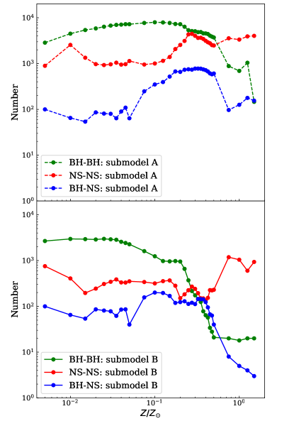
Figure 4: The formation number of mDCOs at different metallicities.

6.3 Fraction of mDCOs formed from ULXs

One can expect that a large fraction of mDCO evolved through an ULX phase because to become short period DCO these systems had to go through various phases involving very high mass-transfer rates (see Belczynski et al., 2017, and references therein).

The number of mDCOs formed from ULXs channels can be very different at different metallicities. $f_{\rm mDCO,ULX}$ represent the percentage of mDCOs that came from ULX channels. For our standard model (submodel B), the values of $f_{\rm mDCO,ULX}$ at different metallicities are shown in Fig. 5. The main feature here is that the percentage of BH-BH and BH-NS systems that went through the wind ULX phase increases with metallicity (upper panel of Fig. 5). This can be understood using the results presented in the previous section (see section 6.1), where we showed that the population of wind BH-ULX remains nearly constant throughout metallicities even though the overall number of binary systems with BH accretors decreases at high metallicities. This indicates that as metallicity increases more BH binary systems have evolved through the wind ULX phase and eventually this will also increase the formation of BH-BH and BH-NS systems through wind ULX channel.

In the case of the NS-NS population, almost none of the close NS-NS systems have evolved through the wind ULX phase. Most of the wind NS-ULXs are in wide orbits and they will not form merging NS-NS systems within Hubble time.

The number of mDCOs that went through the RLOF ULX phase does not behave in a monotonic way with metallicity (bottom panel of Fig. 5). The mDCOs that went through RLOF mass transfer, almost all of them achieved the ULX phase (see Fig. 6). The heavily non-monotonic behavior of $f_{\rm mDCO,ULX}$ of RLOF ULX is caused by various factors that change with metallicity such as the initial orbital separation of DCOs (de Mink & Belczynski, 2015; Klencki et al., 2018), wind mass loss rate that changes orbital separation and radial expansion of the donor star (Belczynski et al., 2010b). These factors determine whether a given system evolves through a RLOF phase and if so, at what evolutionary stage. All together, these factors play a very complex role which leads to the formation of a non-monotonic relation between the number of RLOF systems and metallicity.

We found that only a small percentage of merging BH-BH systems ($0-10\%$) have evolved through the RLOF ULX phase whereas for BH-NS and NS-NS systems the percentage, respectively, varies between $0-71\%$ and $4-100\%$ depending on metallicity. The small fraction of the ULX-descendant merging BH-BHs is due to the fact that the high mass transfer rate RLOF onto compact object is more restricted in case of BH-BH progenitors than for BH-NS and NS-NS progenitors. BH/NS can accrete at high rate (typically) either from a HG donor or from an evolved low-mass He-star. Massive HG stars ($\gtrsim 7\ M_{\odot}$; massive enough to form later a NS or a BH) and low mass He stars ($\sim 2-4\ M_{\odot}$; but massive enough to form later NSs) are subject to significant/rapid radial expansion, leading at favorable binary configurations to RLOF high mass transfer rates and formation of ULXs. Massive He stars ($\gtrsim 4\ M_{\odot}$; that could later form BHs) do not expand significantly (Delgado & Thomas, 1981; Habets, 1987; Avila-Reese, 1993; Woosley et al., 1995; Hurley et al., 2000; Ivanova et al., 2003; Dewi & Pols, 2003) and typically do not lead to high mass transfer RLOF nor to ULX phase. It follows that BH-BH progenitors with RLOF ULX phase are mostly restricted to HG donors, while NS-NS/BH-NS progenitors are allowed to have HG or low mass He star donors making it easier to generate RLOF ULX phase.

We also provide the percentage of total mDCOs that have evolved through the ULX phase (solid black line in Fig. 5). The total curve nearly follows the BH-BH population of wind ULX at low metallicity ($Z\leq 0.25Z_{\odot}$). At low metallicity the mDCO population is dominated by BH-BH systems but as metallicity increases the number of BH-BH systems goes down and NS-NS becomes the major systems in the population of mDCOs (see Fig. 4).

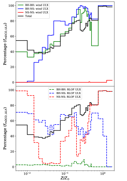
Figure 5: The percentage of different mDCOs that went through different ULX phases at different metallicities in submodel B. Note that at some metallicities sum of wind and RLOF population can be higher than 100%, this means that some ULXs went through both wind and RLOF mass transfer phases. The black line shows percentage of all mDCOs that have evolved through at least one (RLOF or wind) ULX phase.

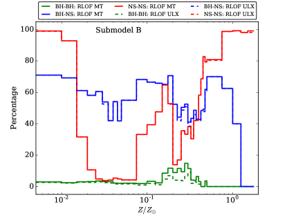
Figure 6: The solid lines show the percentage of mDCOs that went through RLOF mass transfer phase after the first compact object formation and the dotted lines show the percentage of mDCOs that went through RLOF ULX phase.

6.4 Fraction of ULXs that will form mDCOs

We do not expect a large fraction of ULXs to become mDCO or even DCO. According to Wiktorowicz et al. (2017, 2019), ULXs have too low masses of at least one stellar component and/or too long orbital periods to evolve into systems that will be observable by LIGO/Virgo. The study by Wiktorowicz et al. (2017, 2019) was limited to only RLOF ULXs, we note that, the same thing applies to wind ULXs.

Depending on the donor mass, ULXs may, or may not form mDCOs at the end of their evolution. $f_{\text{\tiny ULX,mDCO}}$ represents the percentage of ULXs that forms mDCOs out of the same simulation mass $M_{\rm sim}$. Table 1 shows the values of $f_{\text{\tiny ULX,mDCO}}$ for both submodels A and B. In submodel B, the values of $f_{\text{\tiny ULX,mDCO}}$ are very low: between 1% to 5% depending on metallicity (see also Table 5). In submodel A, $f_{\text{\tiny ULX,mDCO}}$ increases with metallicity, from 4% to 15%. As the different ULX populations remain nearly constant with metallicity (except for RLOF BH-ULXs), the values of $f_{\text{\tiny ULX,mDCO}}$ are simply determined by the number of mDCOs that has evolved through the ULX phase (see section 6.3). In submodel A, $f_{\text{\tiny ULX,mDCO}}$ increases with metallicity because as metallicity increases more number of mDCOs went through the ULX phase. Whereas in submodel B, $f_{\text{\tiny ULX,mDCO}}$ slightly decreases with increasing metallicity simply because as metallicity increases more of mDCO progenitors (some of which are also ULX progenitors) are merged due to the CE phase initiated by an HG donor (Belczynski et al., 2010b).

Next we want to estimate what percentage of the observed ULXs will form mDCOs. Below we describe a model that allows to estimate the fraction of ULXs, weighted by the duration of ULX phase, that will eventually form mDCOs at a given metallicity. The probability of an ULX to be observed is directly proportional to the duration of ULX phase and inversely proportional to the beaming. This model utilizes only the beaming parameter and the lifetime of ULX phase as proxy for observability, but ignores the specific star formation history and the delay time between star formation and the onset of the ULX phase. Note that various ULXs may not only have different duration of high-luminosity phases, but also different delay times. Full models for some specific star formation history and metallicity can be easily constructed with our data and be used to study individual galaxies hosting ULXs. Various galaxies can have very complex chemical evolution and different types of star formation episodes (like burst type, continuous or a combination of both). Our model can only be directly applied to galaxies having simple properties such as a straightforward chemical composition and a constant star formation. $f_{\text{\tiny ULX,mDCO}}^{\text{obs}}$ depends both on the evolution model and the metallicity.

We calculate $f_{\text{\tiny ULX,mDCO}}^{\text{obs}}$ (for $0.01Z_{\odot}$, $0.1Z_{\odot}$ and $Z_{\odot}$) as:

$$f_{\text{\tiny ULX,mDCO}}^{\text{obs}}=\frac{\sum\limits_{i=1}^{n}\text{dt}_{\text{ \tiny ULX,mDCO}}^{i}\times b_{i}}{\sum\limits_{i=1}^{n}\text{dt}_{\text{\tiny ULX}}^{i}\times b_{i}}\times 100\%,$$ (41)

where the numerator represents the sum over the lifetime of ULX phase multiplied with the beaming parameter for ULXs that will form mDCOs at the end and the denominator represents the sum for all ULXs. The values of $f_{\text{\tiny ULX,mDCO}}^{\rm obs}$ are given Table 1. The behavior of $f_{\text{\tiny ULX,mDCO}}^{\rm obs}$ is much more complex than that of $f_{\text{\tiny ULX,mDCO}}$, as it is weighted by the duration of the ULX phase and the beaming parameter which are very different for different type of ULXs. RLOF ULXs tend to have longer ULX phases than wind ULXs. The drop of $f_{\text{\tiny ULX,mDCO}}^{\rm obs}$ at $0.1Z_{\odot}$ is caused by decrease in the number of mDCOs formation through RLOF ULX channel (shown in the bottom panel of Fig. 5).

The duration of the ULX phase depends on the ULX accretor (BH/NS) and the ULX type (RLOF/wind). Table 3 (see the Appendix) shows the average duration of the ULX phase in submodel B. The average duration of the NS-ULXs phase varies between $0.07-0.8$ (depending on metallicity) Myr and for BH-ULXs $0.06-0.4$ Myr. On average RLOF ULXs last $3-38$ times longer than wind ULXs.

Table 1: $f_{\text{\tiny ULX,mDCO}}$ represents the percentage of ULXs that has formed mDCOs while $f_{\text{\tiny ULX,mDCO}}^{\text{obs}}$ (weighted by the duration of ULX phase and beaming) represents the percentage of observed ULXs which will form mDCOs in future.

Model Metallicity $f_{\text{\tiny ULX,mDCO}}^{\text{obs}}$ $f_{\text{ \tiny ULX,mDCO}}$ Submodel A $0.01Z_{\odot}$ 14.0% 4.0% $0.1Z_{\odot}$ 6.9% 7.8% $Z_{\odot}$ 39.7% 10.8% Submodel B $0.01Z_{\odot}$ 14.1% 3.7% $0.1Z_{\odot}$ 4.8% 3.5% $Z_{\odot}$ 20.1% 3.5%

6.5 DCO merger rates

We used the cosmic star formation history (Eq. 1) and the evolution of average metallicity throughout cosmic time (Eq. 4) to calculate the merger rates of mDCOs ($\mathcal{R}_{\rm{mDCO}}$). Fig. 7 shows the merger rate densities at different redshift. The merger rate densities at the local Universe ($z=0$) are given in Table 2. Submodel A gives the optimistic values of merger rates, that are quite high compared to submodel B.

Our BH-BH merger rate density ($53{\rm~{}Gpc}^{-3}{\rm~{}yr}^{-1}$ in submodel B) matches the current LIGO/Virgo constraint from the combined O1/O2 observational runs ($9.7-101{\rm~{}Gpc}^{-3}{\rm~{}yr}^{-1}$; Abbott et al., 2019). However, our current rates are smaller than the rates previously obtained with the StarTrack code for similar evolutionary models (e.g., model M1 submodel B in Belczynski et al., 2016a, $218{\rm~{}Gpc}^{-3}{\rm~{}yr}^{-1}$). Note that early (the beginning of O1) LIGO/Virgo merger rate estimate was much broader ($2-400{\rm~{}Gpc}^{-3}{\rm~{}yr}^{-1}$) than the current O1/O2 estimate. To match the current estimate we have changed our assumption on the IMF slope for massive stars (from $\alpha=-2.3$ to $\alpha=-2.7$) reducing the number of BHs in our simulations. A similar effect can be obtained by altering the chemical evolution model used in calculating the merger rate densities for double compact objects (e.g., our Eq. 4). This alternative solution to matching observational estimates of the merger rates with StarTrack simulations was already demonstrated by Chruslinska et al. (2019) for the LIGO/Virgo sources and by Olejak et al. (2019) for the Galactic populations of double compact-object binaries. Matching the current LIGO/Virgo merger rates for NS-NS and BH-NS mergers turns out to be more difficult than for BH-BH mergers, but it is achievable with various combinations of evolutionary parameters (see Fig. 25 and Fig. 26 of Belczynski et al., 2017).

Next we separately calculated the merger rate densities defined as $\mathcal{R}_{\rm{ULX\rightarrow mDCO}}$ for systems that form mDCOs through ULX channels. Our merger rate calculation can be used to estimate what percentage of mDCO came from ULX channels. We found that in the local Universe, in submodel A, 37% of NS-NS, 56% of BH-NS and 42% of BH-BH mergers came from ULX channels, whereas in submodel B this percentage increases to 62% for NS-NS, 92% for BH-NS and 53% for BH-BH. In submodel B the merger rates (both $\mathcal{R}_{\rm{mDCO}}$ and $\mathcal{R}_{\rm{ULX\rightarrow mDCO}}$) go down due to the merger of binary system during CE, initiated by HG donors. In submodel B, even though $\mathcal{R}_{\rm{mDCO}}$ and $\mathcal{R}_{\rm{ULX\rightarrow mDCO}}$ decrease, the fraction $\mathcal{R}_{\rm{ULX\rightarrow mDCO}}/\mathcal{R}_{\rm{mDCO}}$ increases compared to submodel A (see Table 2). It indicates that lower fraction of ULXs went through CE phase with HG donors than the fraction of mDCOs.

Table 2: Estimated merger rate densities at the local Universe ($z=0$). $\mathcal{R}_{\rm{mDCO}}$ represents the merger rate densities for mDCOs while $\mathcal{R}_{\rm{ULX\rightarrow mDCO}}$ represents the merger rate densities for the mDCOs that are formed through ULX channels.

Model DCO type $\mathcal{R}_{\rm{mDCO}}$ $\mathcal{R}_{\rm{ULX\rightarrow mDCO}}$ Percentage $\rm{Gpc^{-3}\ yr^{-1}}$ $\small\rm{Gpc^{-3}\ yr^{-1}}$ Submodel A NS-NS 128.02 48.25 37.68% BH-NS 30.12 17.02 56.5% BH-BH 296.46 127.25 42.92% Submodel B NS-NS 32.36 20.2 62.4% BH-NS 6.34 5.86 92.4% BH-BH 53.24 28.25 53%

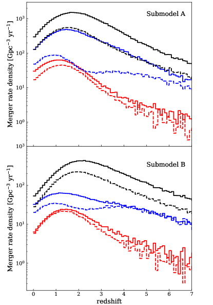
Figure 7: DCO merger rate density at different redshift. Black, blue and red solid lines represent BH-BH, NS-NS, and BH-NS merger rate densities, respectively. Black, blue and red dash lines show merger rate densities of BH-BH, NS-NS and BH-NS systems that undergone an ULX phase in their evolution.

7 Conclusions

We did a study of a subset of X-ray binaries – those that went through the ULX phase – and we focused on ones that form mDCOs at the end. We incorporated super-critical mass accretion onto a compact object and physically motivated beaming in our population synthesis study of large number of binary systems. ULX populations studied in this paper do not represent the complete sample of ULX, as ULXs containing Be star companions are not included in this work. The conclusions based on the restricted population of ULXs are listed below.

• ULXs can host both NSs and BHs as accretors. The average life time of the NS-ULX phase varies between $0.07-0.8$ (depending on metallicity) Myr and for BH-ULX $0.06-0.4$ Myr (see Table 3). As NS-ULXs are more prone to be beamed (King & Lasota, 2016; Wiktorowicz et al., 2019), we obtained (weighted by beaming and life time of ULX phase) that the number of NS-ULXs would be $0.1-1$ (depending on metallicity) times of BH-ULXs in the observed sample of ULXs. Our estimate may be compared with that of Middleton & King (2017), who found that in the observed sample, the number of NS-ULXs would be $\sim 0.1-0.4$ times of BH-ULXs.

• ULXs can be powered by both RLOF and wind mass transfer. In submodel B, on average RLOF ULXs last $3-38$ ($1-31$ times in submodel A) times longer than wind ULXs (see Table 3).

• The number of RLOF BH-ULXs decreases at high metallicity while the number of wind BH-ULXs remains almost constant in all tested metallicities ($Z=0.005Z_{\odot}$ to $Z=1.5Z_{\odot}$). The number of NS-ULXs (both RLOF and wind) does not depend much on metallicity.

• The average mass of donor and accretor in BH-ULXs (both RLOF and wind) decreases as metallicity increases. The average donor mass in RLOF BH-ULXs is 9.3 $M_{\odot}$, 6.7 $M_{\odot}$, and 2.2 $M_{\odot}$ for $Z=0.01Z_{\odot}$, $0.1Z_{\odot}$ and $Z_{\odot}$ respectively. The average BH mass in RLOF BH-ULXs is 18.5 $M_{\odot}$, 15.3 $M_{\odot}$, and 8.2 $M_{\odot}$ for $Z=0.01Z_{\odot}$, $0.1Z_{\odot}$ and $Z_{\odot}$, respectively.

• The average donor mass in wind and RLOF NS-ULXs is $\sim 1.25\ M_{\odot}$ and $\sim 1.0\ M_{\odot}$, respectively, almost independent of metallicity.

• The fraction of ULXs that forms mDCOs ($f_{\text{\tiny ULX,mDCO}}$), potential LIGO/Virgo sources, depends both on CE outcome and metallicity. In our standard CE model (submodel B), the fraction is very low ($\sim 3.5\%$) but in our optimistic CE model (submodel A) where CE events from the HG donor are allowed, the fraction is higher and increases with metallicity (4.0%, 7.8%, 10.8% for $Z=0.01Z_{\odot}$, $0.1Z_{\odot}$, $Z_{\odot}$, respectively).

• Our calculation of $f_{\text{\tiny ULX,mDCO}}^{\text{obs}}$ which is weighted by the duration of the ULX phase and beaming shows that $5-40\%$ (depending on CE model and metallicity) of the observed ULXs will form mDCOs in future.

• From our cosmic merger rate calculation of mDCOs (see Fig. 7), one can predict how many of the merging LIGO/Virgo sources came from ULX channels. We found that in the local Universe ($z=0$) the majority of the DCO mergers formed from isolated binaries went through a ULX phase. The numbers in two different submodel A/B are $37\%/62\%$ for merging NS-NS, $56\%/92\%$ for merging BH-NS and $42\%/53\%$ for merging BH-BH.

8 ACKNOWLEDGMENTS

We thank the anonymous referee for constructive and very useful comments. KB, JPL and SM acknowledge support from the Polish National Science Center (NCN) grants: UMO-2015/19/B/ST9/01099. KB and SM were also partially supported by NCN Maestro grant 2018/30/A/ST9/00050. JPL was supported in part by a grant from the French Spatial Agency CNES. ARK thanks the Institut d’Astrophysique, Paris for visiting support.

Appendix A SIMULATION OUTPUT

As mentioned earlier in the paper we have simulated $2\times 10^{6}$ binary star in 32 different metallicity from $Z=0.005Z_{\odot}$ to $Z=1.5Z_{\odot}$. Table 3 shows the average duration of the ULX phase. The detailed numerical outputs from our simulation are summarized in Table 4 and 5. Table 4 contains the formation number of different type of ULXs and DCOs. The formation efficiencies are also given in Table 4. Table 5 contains the most necessary informations concerning the connection between ULX and DCO. The percentage of ULXs that ends up forming DCOs and the percentage of DCOs that came from ULX channels both numbers are given in Table 5.

Table 3:

The average lifetime of the ULX phase for different type of ULXs in submodel B. $\tau$ is the average lifetime of the ULX phase in Myr. RLOF and wind ULX represent the mass transfer mode in ULX. The subscript of $\tau$ denotes the accretor type in ULXs.

Z	RLOF ULX			wind ULX			$\tau_{\rm NS(RLOF+wind)}$	$\tau_{\rm BH(RLOF+wind)}$
	$\tau_{\rm NS}$	$\tau_{\rm BH}$	$\tau_{\rm NS+BH}$	$\tau_{\rm NS}$	$\tau_{\rm BH}$	$\tau_{\rm NS+BH}$
0.005$Z_{\odot}$	0.210	1.046	0.524	0.016	0.104	0.049	0.079	0.407
0.01$Z_{\odot}$	0.174	0.909	0.354	0.016	0.128	0.056	0.068	0.301
0.015$Z_{\odot}$	0.641	1.247	0.874	0.017	0.104	0.052	0.200	0.426
0.02$Z_{\odot}$	1.108	0.846	0.988	0.018	0.095	0.049	0.322	0.337
0.025$Z_{\odot}$	1.433	0.834	1.143	0.019	0.091	0.050	0.424	0.343
0.03$Z_{\odot}$	1.532	0.850	1.209	0.020	0.089	0.050	0.469	0.343
0.035$Z_{\odot}$	1.918	0.887	1.441	0.021	0.090	0.051	0.594	0.345
0.04$Z_{\odot}$	1.976	1.091	1.576	0.020	0.092	0.052	0.608	0.398
0.045$Z_{\odot}$	2.645	1.078	1.957	0.020	0.094	0.052	0.802	0.394
0.05$Z_{\odot}$	2.018	1.337	1.729	0.020	0.096	0.052	0.596	0.454
0.075$Z_{\odot}$	0.876	1.056	0.959	0.031	0.062	0.051	0.451	0.383
0.1$Z_{\odot}$	0.788	1.214	0.977	0.030	0.065	0.053	0.427	0.405
0.125$Z_{\odot}$	0.655	1.405	0.948	0.029	0.072	0.056	0.347	0.439
0.15$Z_{\odot}$	0.692	1.400	0.926	0.032	0.093	0.070	0.384	0.432
0.175$Z_{\odot}$	1.277	1.726	1.419	0.029	0.115	0.076	0.565	0.472
0.2$Z_{\odot}$	1.186	1.692	1.352	0.024	0.131	0.078	0.384	0.408
0.225$Z_{\odot}$	0.752	1.836	1.047	0.020	0.126	0.067	0.211	0.367
0.25$Z_{\odot}$	0.535	2.356	0.964	0.017	0.126	0.062	0.139	0.388
0.275$Z_{\odot}$	0.612	2.367	1.027	0.018	0.117	0.059	0.156	0.379
0.3$Z_{\odot}$	0.378	1.966	0.774	0.019	0.105	0.056	0.107	0.335
0.325$Z_{\odot}$	0.537	1.751	0.873	0.021	0.104	0.058	0.150	0.326
0.35$Z_{\odot}$	0.698	1.486	0.913	0.022	0.099	0.057	0.205	0.296
0.375$Z_{\odot}$	0.665	1.560	0.897	0.024	0.096	0.057	0.203	0.299
0.4$Z_{\odot}$	0.734	1.526	0.917	0.025	0.089	0.056	0.239	0.266
0.425$Z_{\odot}$	0.710	1.349	0.843	0.027	0.082	0.054	0.250	0.227
0.45$Z_{\odot}$	0.645	0.990	0.703	0.028	0.077	0.052	0.251	0.170
0.475$Z_{\odot}$	0.534	0.801	0.576	0.028	0.073	0.050	0.215	0.145
0.5$Z_{\odot}$	0.608	0.597	0.607	0.028	0.069	0.049	0.243	0.112
0.75$Z_{\odot}$	0.150	1.689	0.206	0.028	0.060	0.042	0.096	0.150
$Z_{\odot}$	0.150	1.387	0.168	0.030	0.055	0.046	0.104	0.071
1.25$Z_{\odot}$	0.124	0.505	0.127	0.030	0.064	0.047	0.089	0.070
1.5$Z_{\odot}$	0.123	0.337	0.124	0.027	0.058	0.039	0.086	0.060

Table 4:

The number of different systems formed from simulation of $2\times 10^{6}$ binary stars at each metallicity in submodel B. The corresponding simulation mass is $M_{\rm sim}=4.4\times 10^{8}M_{\odot}$ . ULX^R and ULX^W represent the number of ULX systems formed during RLOF and wind mass transfer episodes, respectively. NS-NS, BH-NS and BH-BH represent the number of mDCOs.

Z	NS-ULXR	BH-ULXR	$\frac{\text{ULX${}^{R}$}}{M_{\rm sim}}$	NS-ULXW	BH-ULXW	$\frac{\text{ULX${}^{W}$}}{M_{\rm sim}}$	NS-NS	$\frac{\text{NS-NS}}{M_{\rm sim}}$	BH-NS	$\frac{\text{BH-NS}}{M_{\rm sim}}$	BH-BH	$\frac{\text{BH-BH}}{M_{\rm sim}}$
0.005$Z_{\odot}$	8545	5141	3.1e-05	17638	10846	6.4e-05	754	1.7e-06	100	2.2e-07	2672	6e-06
0.01$Z_{\odot}$	8646	2818	2.6e-05	17483	9878	6.2e-05	407	9.1e-07	65	1.5e-07	2967	6.7e-06
0.015$Z_{\odot}$	6830	4267	2.5e-05	16499	10878	6.2e-05	196	4.4e-07	54	1.2e-07	2935	6.6e-06
0.02$Z_{\odot}$	6266	5248	2.6e-05	16186	11037	6.1e-05	244	5.5e-07	86	1.9e-07	2884	6.5e-06
0.025$Z_{\odot}$	6248	5886	2.7e-05	15590	11507	6.1e-05	308	6.9e-07	81	1.8e-07	2979	6.7e-06
0.03$Z_{\odot}$	6226	5612	2.7e-05	14739	11236	5.8e-05	344	7.7e-07	78	1.8e-07	2907	6.5e-06
0.035$Z_{\odot}$	6130	5288	2.6e-05	14159	11198	5.7e-05	387	8.7e-07	62	1.4e-07	2846	6.4e-06
0.04$Z_{\odot}$	6006	4947	2.5e-05	13989	11216	5.7e-05	333	7.5e-07	85	1.9e-07	2567	5.8e-06
0.045$Z_{\odot}$	5796	4535	2.3e-05	13664	10337	5.4e-05	331	7.4e-07	86	1.9e-07	2421	5.4e-06
0.05$Z_{\odot}$	5610	4132	2.2e-05	13849	10177	5.4e-05	352	7.9e-07	40	9e-08	2268	5.1e-06
0.075$Z_{\odot}$	7240	6220	3e-05	7308	13036	4.6e-05	340	7.6e-07	157	3.5e-07	1607	3.6e-06
0.1$Z_{\odot}$	6982	5569	2.8e-05	6343	13215	4.4e-05	317	7.1e-07	200	4.5e-07	1241	2.8e-06
0.125$Z_{\odot}$	7108	4562	2.6e-05	6886	12021	4.2e-05	355	8e-07	196	4.4e-07	975	2.2e-06
0.15$Z_{\odot}$	7350	3641	2.5e-05	6442	10408	3.8e-05	368	8.3e-07	169	3.8e-07	960	2.2e-06
0.175$Z_{\odot}$	5961	2770	2e-05	7917	9745	4e-05	282	6.3e-07	119	2.7e-07	976	2.2e-06
0.2$Z_{\odot}$	4270	2092	1.4e-05	9514	9701	4.3e-05	151	3.4e-07	124	2.8e-07	952	2.1e-06
0.225$Z_{\odot}$	3944	1473	1.2e-05	11146	8989	4.5e-05	183	4.1e-07	129	2.9e-07	659	1.5e-06
0.25$Z_{\odot}$	3678	1132	1.1e-05	11995	8483	4.6e-05	225	5.1e-07	113	2.5e-07	371	8.3e-07
0.275$Z_{\odot}$	3587	1111	1.1e-05	11834	8444	4.6e-05	270	6.1e-07	120	2.7e-07	216	4.9e-07
0.3$Z_{\odot}$	3561	1184	1.1e-05	10938	8404	4.3e-05	241	5.4e-07	112	2.5e-07	174	3.9e-07
0.325$Z_{\odot}$	3416	1308	1.1e-05	10182	8386	4.2e-05	194	4.4e-07	145	3.3e-07	145	3.3e-07
0.35$Z_{\odot}$	3507	1312	1.1e-05	9469	7966	3.9e-05	150	3.4e-07	144	3.2e-07	125	2.8e-07
0.375$Z_{\odot}$	3472	1216	1.1e-05	8931	7559	3.7e-05	149	3.3e-07	142	3.2e-07	78	1.8e-07
0.4$Z_{\odot}$	3511	1055	1e-05	8139	7500	3.5e-05	134	3e-07	124	2.8e-07	64	1.4e-07
0.425$Z_{\odot}$	3690	968	1e-05	7623	7451	3.4e-05	153	3.4e-07	95	2.1e-07	57	1.3e-07
0.45$Z_{\odot}$	4169	834	1.1e-05	7372	7338	3.3e-05	226	5.1e-07	67	1.5e-07	34	7.6e-08
0.475$Z_{\odot}$	4184	775	1.1e-05	7131	7060	3.2e-05	223	5e-07	63	1.4e-07	28	6.3e-08
0.5$Z_{\odot}$	4177	641	1.1e-05	7092	7199	3.2e-05	230	5.2e-07	40	9e-08	21	4.7e-08
0.75$Z_{\odot}$	9545	363	2.2e-05	7573	6196	3.1e-05	1184	2.7e-06	8	1.8e-08	20	4.5e-08
$Z_{\odot}$	10617	157	2.4e-05	6593	13048	4.4e-05	1043	2.3e-06	5	1.1e-08	18	4e-08
1.25$Z_{\odot}$	10850	98	2.5e-05	6533	6529	2.9e-05	600	1.3e-06	4	9e-09	20	4.5e-08
1.5$Z_{\odot}$	11496	39	2.6e-05	7245	4591	2.7e-05	933	2.1e-06	3	6.7e-09	20	4.5e-08

Table 5:

NS-NS, NS-BH and BH-BH represent the number of mDCOs that went through an ULX phase. ULX^R and ULX^W represent RLOF and wind ULX phases, respectively. 4th column shows the number of systems that went through both ULX^R and ULX^W phases. $f_{\text{\tiny ULX,mDCO}}$ shows the percentage of ULXs that forms mDCOs and $f_{\text{\tiny mDCO,ULX}}$ shows what percentage of mDCOs came from ULX channels. This table has been given for submodel B.

Z	ULXR			ULXW			ULXR and ULXW			$f_{\text{\tiny ULX,mDCO}}$	$f_{\text{\tiny mDCO,ULX}}$
	NS-NS	BH-NS	BH-BH	NS-NS	BH-NS	BH-BH	NS-NS	BH-NS	BH-BH
0.005$Z_{\odot}$	746	71	70	0	0	1063	0	0	29	4.6%	54.8%
0.01$Z_{\odot}$	378	45	66	0	1	975	0	1	21	3.7%	41.9%
0.015$Z_{\odot}$	62	33	81	0	14	1100	0	14	36	3.2%	38.9%
0.02$Z_{\odot}$	26	50	77	0	25	1136	0	25	55	3.2%	38.3%
0.025$Z_{\odot}$	15	49	91	0	37	1168	0	34	74	3.2%	37.1%
0.03$Z_{\odot}$	13	41	74	0	34	1227	0	29	71	3.4%	38.7%
0.035$Z_{\odot}$	16	26	65	0	38	1241	0	21	57	3.6%	39.7%
0.04$Z_{\odot}$	18	46	43	0	52	1281	0	34	39	3.8%	45.8%
0.045$Z_{\odot}$	16	36	37	0	53	1164	0	21	28	3.7%	44.2%
0.05$Z_{\odot}$	15	22	38	0	32	1205	0	20	34	3.7%	47.2%
0.075$Z_{\odot}$	113	107	16	0	125	1013	0	88	15	3.8%	60.4%
0.1$Z_{\odot}$	125	133	25	0	149	820	0	102	25	3.5%	64.0%
0.125$Z_{\odot}$	169	129	11	0	150	689	0	101	11	3.4%	67.9%
0.15$Z_{\odot}$	238	110	46	0	144	746	0	93	46	4.1%	76.5%
0.175$Z_{\odot}$	148	84	68	0	101	826	0	73	68	4.1%	78.8%
0.2$Z_{\odot}$	21	65	39	0	118	843	0	61	39	3.9%	80.3%
0.225$Z_{\odot}$	31	54	27	0	126	627	0	52	27	3.1%	80.9%
0.25$Z_{\odot}$	80	55	14	0	113	289	0	55	14	1.9%	67.9%
0.275$Z_{\odot}$	90	61	14	0	119	194	0	60	14	1.6%	66.6%
0.3$Z_{\odot}$	92	43	16	0	108	159	0	41	16	1.5%	68.5%
0.325$Z_{\odot}$	59	62	3	0	143	140	0	62	3	1.5%	70.6%
0.35$Z_{\odot}$	63	66	4	0	140	116	0	62	4	1.5%	77.0%
0.375$Z_{\odot}$	63	60	2	0	137	67	0	57	2	1.3%	73.1%
0.4$Z_{\odot}$	78	52	1	0	114	57	0	44	1	1.3%	79.8%
0.425$Z_{\odot}$	105	45	0	1	79	46	1	31	0	1.2%	80.0%
0.45$Z_{\odot}$	187	32	0	0	59	23	0	27	0	1.4%	83.7%
0.475$Z_{\odot}$	177	38	1	0	57	22	0	33	1	1.4%	83.1%
0.5$Z_{\odot}$	185	28	0	0	33	10	0	21	0	1.2%	80.7%
0.75$Z_{\odot}$	1169	5	0	0	8	20	0	5	0	5.1%	98.7%
$Z_{\odot}$	1034	2	0	0	5	18	0	2	0	3.5%	99.1%
1.25$Z_{\odot}$	589	0	0	16	4	20	16	0	0	2.6%	98.2%
1.5$Z_{\odot}$	925	0	0	25	3	20	25	0	0	4.1%	98.2%

References

- Abbott et al. (2016) Abbott, B. P., Abbott, R., Abbott, T. D., et al. 2016, Physical Review Letters, 116, 061102
- Abbott et al. (2019) Abbott, B. P., Abbott, R., Abbott, T. D., et al. 2019, Physical Review X, 9, 031040
- Askar et al. (2017) Askar, A., Szkudlarek, M., Gondek-Rosińska, D., Giersz, M., & Bulik, T. 2017, MNRAS, 464, L36
- Avila-Reese (1993) Avila-Reese, V. 1993, Revista Mexicana de Astronomia y Astrofisica, 25, 79
- Bachetti et al. (2014) Bachetti, M., Harrison, F. A., Walton, D. J., et al. 2014, Nature, 514, 202
- Banerjee (2018) Banerjee, S. 2018, MNRAS, 473, 909
- Belczynski et al. (2002) Belczynski, K., Kalogera, V., & Bulik, T. 2002, ApJ, 572, 407
- Belczynski et al. (2008a) Belczynski, K., Kalogera, V., Rasio, F. A., et al. 2008a, ApJS, 174, 223
- Belczynski et al. (2008b) Belczynski, K., Taam, R. E., Rantsiou, E., & van der Sluys, M. 2008b, ApJ, 682, 474
- Belczynski et al. (2010a) Belczynski, K., Bulik, T., Fryer, C. L., et al. 2010a, ApJ, 714, 1217
- Belczynski et al. (2010b) Belczynski, K., Dominik, M., Bulik, T., et al. 2010b, ApJ, 715, L138
- Belczynski et al. (2012) Belczynski, K., Wiktorowicz, G., Fryer, C. L., et al. 2012, ApJ, 757, 91
- Belczynski et al. (2016a) Belczynski, K., Holz, D. E., Bulik, T., & O’Shaughnessy, R. 2016a, Nature, 534, 512
- Belczynski et al. (2016b) Belczynski, K., Heger, A., Gladysz, W., et al. 2016b, A&A, 594, A97
- Belczynski et al. (2017) Belczynski, K., Klencki, J., Meynet, G., et al. 2017, arXiv:1706.07053
- Binder et al. (2016) Binder, B., Williams, B. F., Kong, A. K. H., et al. 2016, MNRAS, 457, 1636
- Bondi & Hoyle (1944) Bondi, H., & Hoyle, F. 1944, MNRAS, 104, 273
- Carpano et al. (2018) Carpano, S., Haberl, F., Maitra, C., et al. 2018, MNRAS, 476, L45
- Chatterjee et al. (2017) Chatterjee, S., Rodriguez, C. L., Kalogera, V., & Rasio, F. A. 2017, ApJ, 836, L26
- Chruslinska et al. (2019) Chruslinska, M., Nelemans, G., & Belczynski, K. 2019, MNRAS, 482, 5012
- Colbert & Mushotzky (1999) Colbert, E. J. M., & Mushotzky, R. F. 1999, ApJ, 519, 89
- Delgado & Thomas (1981) Delgado, A. J., & Thomas, H.-C. 1981, Astronomy and Astrophysics, 96, 142
- de Mink & Belczynski (2015) de Mink, S. E., & Belczynski, K. 2015, ApJ, 814, 58
- de Mink & Mandel (2016) de Mink, S. E., & Mandel, I. 2016, MNRAS, 460, 3545
- Dewi & Pols (2003) Dewi, J. D. M., & Pols, O. R. 2003, Monthly Notices of the Royal Astronomical Society, 344, 629
- Dominik et al. (2012) Dominik, M., Belczynski, K., Fryer, C., et al. 2012, ApJ, 759, 52
- Doroshenko et al. (2018) Doroshenko, V., Tsygankov, S., & Santangelo, A. 2018, A&A, 613, A19
- Duchêne & Kraus (2013) Duchêne, G., & Kraus, A. 2013, ARA&A, 51, 269
- Dvorkin et al. (2015) Dvorkin, I., Silk, J., Vangioni, E., et al. 2015, MNRAS, 452, L36
- Feng & Soria (2011) Feng, H., & Soria, R. 2011, New Astron. Rev., 55, 166
- Finke & Razzaque (2017) Finke, J. D., & Razzaque, S. 2017, MNRAS, 472, 3683
- Fortin et al. (2016) Fortin, M., Providência, C., Raduta, A. R., et al. 2016, Phys. Rev. C, 94, 035804
- Fryer et al. (2012) Fryer, C. L., Belczynski, K., Wiktorowicz, G., et al. 2012, ApJ, 749, 91
- Fürst et al. (2016) Fürst, F., Walton, D. J., Harrison, F. A., et al. 2016, ApJ, 831, L1
- Fürst et al. (2017) Fürst, F., Walton, D. J., Stern, D., et al. 2017, ApJ, 834, 77
- Habets (1987) Habets, G. M. H. J. 1987, Astronomy and Astrophysics Supplement Series, 69, 183
- Heida et al. (2015) Heida, M., Torres, M. A. P., Jonker, P. G., et al. 2015, MNRAS, 453, 3510
- Heida et al. (2016) Heida, M., Jonker, P. G., Torres, M. A. P., et al. 2016, MNRAS, 459, 771
- Hobbs et al. (2005) Hobbs, G., Lorimer, D. R., Lyne, A. G., et al. 2005, MNRAS, 360, 974
- Hurley et al. (2000) Hurley, J. R., Pols, O. R., & Tout, C. A. 2000, Monthly Notices of the Royal Astronomical Society, 315, 543
- Hurley et al. (2002) Hurley, J. R., Tout, C. A., & Pols, O. R. 2002, MNRAS, 329, 897
- Israel et al. (2017a) Israel, G. L., Belfiore, A., Stella, L., et al. 2017a, Science, 355, 817
- Israel et al. (2017b) Israel, G. L., Papitto, A., Esposito, P., et al. 2017b, MNRAS, 466, L48
- Ivanova & Taam (2004) Ivanova, N., & Taam, R. E. 2004, ApJ, 601, 1058
- Ivanova et al. (2003) Ivanova, N., Belczynski, K., Kalogera, V., et al. 2003, The Astrophysical Journal, 592, 475
- Ivanova et al. (2013) Ivanova, N., Justham, S., Chen, X., et al. 2013, A&ARv, 21, 59
- Kaaret et al. (2017) Kaaret, P., Feng, H., & Roberts, T. P. 2017, ARA&A, 55, 303
- King & Begelman (1999) King, A. R., & Begelman, M. C. 1999, ApJ, 519, L169
- King & Ritter (1999) King, A. R., & Ritter, H. 1999, MNRAS, 309, 253
- King et al. (2001) King, A. R., Davies, M. B., Ward, M. J., Fabbiano, G., & Elvis, M. 2001, ApJ, 552, L109
- King & Wijnands (2006) King A. R., Wijnands R., 2006, MNRAS, 366, L31
- King (2009) King, A. R. 2009, MNRAS, 393, L41
- King & Lasota (2016) King, A., & Lasota, J.-P. 2016, MNRAS, 458, L10
- King & Lasota (2019) King, A., & Lasota, J.-P. 2019, MNRAS, 485, 3588
- King et al. (2017) King, A., Lasota, J.-P., & Kluźniak, W. 2017, MNRAS, 468, L59
- Klencki & Nelemans (2018) Klencki, J., & Nelemans, G. 2018, arXiv e-prints, arXiv:1812.00012
- Klencki et al. (2018) Klencki, J., Moe, M., Gladysz, W., et al. 2018, A&A, 619, A77
- Kroupa et al. (1993) Kroupa, P., Tout, C. A., & Gilmore, G. 1993, MNRAS, 262, 545
- Kruckow et al. (2018) Kruckow, M. U., Tauris, T. M., Langer, N., Kramer, M., & Izzard, R. G. 2018, MNRAS, 481, 1908
- Lasota et al. (2011) Lasota, J.-P., Alexander, T., Dubus, G., et al. 2011, ApJ, 735, 89
- Lee et al. (1991) Lee, U., Osaki, Y., & Saio, H. 1991, MNRAS, 250, 432
- Liu et al. (2007) Liu, Q. Z., van Paradijs, J., & van den Heuvel, E. P. J. 2007, A&A, 469, 807
- Madau & Dickinson (2014) Madau, P., & Dickinson, M. 2014, ARA&A, 52, 415
- Mandel & de Mink (2016) Mandel, I., & de Mink, S. E. 2016, MNRAS, 458, 2634
- Marchant et al. (2016) Marchant, P., Langer, N., Podsiadlowski, P., et al. 2016, A&A, 588, A50
- Marchant et al. (2017) Marchant, P., Langer, N., Podsiadlowski, P., et al. 2017, A&A, 604, A55
- Martin et al. (2014) Martin, R. G., Nixon, C., Armitage, P. J., et al. 2014, ApJ, 790, L34
- Middleton & King (2017) Middleton, M. J., & King, A. 2017, MNRAS, 470, L69
- Mineo et al. (2012) Mineo, S., Gilfanov, M., & Sunyaev, R. 2012, MNRAS, 419, 2095
- Motch et al. (2011) Motch, C., Pakull, M. W., Grisé, F., & Soria, R. 2011, Astronomische Nachrichten, 332, 367
- Motch et al. (2014) Motch, C., Pakull, M. W., Soria, R., Grisé, F., & Pietrzyński, G. 2014, Nature, 514, 198
- Negueruela (1998) Negueruela, I. 1998, A&A, 338, 505
- Negueruela et al. (2001) Negueruela, I., Okazaki, A. T., Fabregat, J., et al. 2001, A&A, 369, 117
- Negueruela & Okazaki (2001) Negueruela, I., & Okazaki, A. T. 2001, A&A, 369, 108
- Olejak et al. (2019) Olejak, A., Belczynski, K., Bulik, T., et al. 2019, arXiv e-prints, arXiv:1908.08775
- Pavlovskii et al. (2017) Pavlovskii, K., Ivanova, N., Belczynski, K., et al. 2017, MNRAS, 465, 2092
- Portegies Zwart et al. (2004) Portegies Zwart, S. F., Baumgardt, H., Hut, P., Makino, J., & McMillan, S. L. W. 2004, Nature, 428, 724
- Rodriguez et al. (2016) Rodriguez, C. L., Chatterjee, S., & Rasio, F. A. 2016, Phys. Rev. D, 93, 084029
- Sana et al. (2013) Sana, H., de Koter, A., de Mink, S. E., et al. 2013, A&A, 550, A107
- Soria et al. (2005) Soria, R., Cropper, M., Pakull, M., Mushotzky, R., & Wu, K. 2005, MNRAS, 356, 12
- Shakura & Sunyaev (1973) Shakura, N. I., & Sunyaev, R. A. 1973, A&A, 24, 337
- Swartz et al. (2011) Swartz, D. A., Soria, R., Tennant, A. F., et al. 2011, ApJ, 741, 49
- Townsend et al. (2017) Townsend, L. J., Kennea, J. A., Coe, M. J., et al. 2017, MNRAS, 471, 3878
- Trudolyubov et al. (2007) Trudolyubov, S. P., Priedhorsky, W. C., & Córdova, F. A. 2007, ApJ, 663, 487
- Trudolyubov (2008) Trudolyubov, S. P. 2008, MNRAS, 387, L36
- Tsygankov et al. (2017) Tsygankov, S. S., Doroshenko, V., Lutovinov, A. A., et al. 2017, A&A, 605, A39
- Tutukov & Yungelson (1993) Tutukov, A. V., & Yungelson, L. R. 1993, MNRAS, 260, 675
- Vangioni et al. (2015) Vangioni, E., Olive, K. A., Prestegard, T., et al. 2015, MNRAS, 447, 2575
- Vagnozzi et al. (2017) Vagnozzi, S., Freese, K., & Zurbuchen, T. H. 2017, ApJ, 839, 55
- Vasilopoulos et al. (2018) Vasilopoulos, G., Haberl, F., Carpano, S., et al. 2018, A&A, 620, L12
- Venumadhav et al. (2019) Venumadhav, T., Zackay, B., Roulet, J., et al. 2019, arXiv e-prints , arXiv:1904.07214
- Vink et al. (2001) Vink, J. S., de Koter, A., & Lamers, H. J. G. L. M. 2001, A&A, 369, 574
- Vink & de Koter (2005) Vink, J. S., & de Koter, A. 2005, A&A, 442, 587
- Weng et al. (2017) Weng, S.-S., Ge, M.-Y., Zhao, H.-H., et al. 2017, ApJ, 843, 69
- Wiktorowicz et al. (2014) Wiktorowicz, G., Belczynski, K., & Maccarone, T. 2014, Binary Systems, Their Evolution and Environments, 37
- Wiktorowicz et al. (2015) Wiktorowicz, G., Sobolewska, M., Sa̧dowski, A., & Belczynski, K. 2015, ApJ, 810, 20
- Wiktorowicz et al. (2017) Wiktorowicz, G., Sobolewska, M., Lasota, J.-P., & Belczynski, K. 2017, ApJ, 846, 17
- Wiktorowicz et al. (2019) Wiktorowicz, G., Lasota, J.-P., Middleton, M., et al. 2019, ApJ, 875, 53
- Woosley et al. (1995) Woosley, S. E., Langer, N., & Weaver, T. A. 1995, The Astrophysical Journal, 448, 315
- Zorec & Briot (1997) Zorec, J., & Briot, D. 1997, A&A, 318, 443