Almost Perfect Metals in One Dimension

Abstract

We show that a one-dimensional quantum wire with as few as 2 channels of interacting fermions can host metallic states of matter that are stable against all perturbations up to $q^{\text{th}}$-order in fermion creation/annihilation operators for any fixed finite $q$. The leading relevant perturbations are thus complicated operators that are expected to modify the physics only at very low energies, below accessible temperatures. The stability of these non-Fermi liquid fixed points is due to strong interactions between the channels, which can (but need not) be chosen to be purely repulsive. Our results might enable elementary physical realizations of these phases.

Introduction. Metallic states of matter are gapless and often unstable to either insulating behavior or superconductivity. This is especially true in one-dimensional systems, where the localizing effects of disorder are particularly strong Lee and Ramakrishnan (1985). For a single channel (i.e. a single propagating mode of each chirality at the Fermi energy), disorder-induced localization can only be avoided when the interaction is strongly attractive, while proximity-induced superconductivity can only be avoided when it is strongly repulsive Giamarchi (2003). The situation is more complicated—and much more interesting—when there are multiple channels. We will show that, surprisingly, even for $N=2$ channels, it is possible to have a metallic state that is stable against all perturbations up to $q^{\text{th}}$-order in fermion creation/annihilation operators for any fixed finite $q$ (but not $q=\infty$), which we call (absolute) $q$-stability.

Gapless phases of interacting fermions in one dimension are described at low energies by Luttinger liquid (LL) theory Haldane (1981). They exhibit a remarkable and universal phenomenology that distinguishes them from Fermi liquids, but this is often obscured in experiments due to dimensional crossover, ordering, or localization Giamarchi (2003). Thus, a physically realizable stable LL is not only interesting as a matter of principle, but also for the practical reason that it would provide a useful experimental platform to study non-Fermi liquid physics.

For $N=\infty$, it was shown two decades ago in Refs. Kivelson et al. (1998); Golubović and Golubović (1998); O’Hern and Lubensky (1998); O’Hern et al. (1999); Emery et al. (2000); Vishwanath and Carpentier (2001); Mukhopadhyay et al. (2001); Sierra and Kim (2002) that there exist “sliding Luttinger liquid” phases which are stable against many, but not all, low-order perturbations; it was argued that the relevant perturbations are likely to have small bare values . More recently, it was discovered that it is possible for a one-dimensional metal to be stable against all non-chiral perturbations (without restriction on the order) Plamadeala et al. (2014). An explicit construction was given for $N=23$ which exploited the properties of integral quadratic lattices. The present work shows that a slight relaxation of the condition of complete stability to the weaker condition of $q$-stability brings the required number of channels down from $23$ to $2$, thereby greatly increasing the chances of experimental realization.

The basic observation underlying the results of this paper and of Ref. Plamadeala et al. (2014) is that the possible perturbations of an $N$-channel LL can be represented as lattice points in a fictitious $2N$-dimensional space equipped with two different metrics: the mixed-signature $(N,N)$ metric $\mathrm{diag}(-\mathbb{I}_{N},\mathbb{I}_{N})$ and the Euclidean metric $\mathbb{I}_{2N}$, where $\mathbb{I}_{N}$ is the $N\times N$ identity matrix. The mixed-signature interval from the origin to a lattice point measures the chirality of the associated perturbation, while the Euclidean interval measures its scaling dimension; points sufficiently far from the origin are irrelevant in the renormalization group (RG) sense. The lattice is naturally graded into “shells” consisting of perturbations of a given order; low-order perturbations belong to the inner shells. The effect of interactions is to deform the lattice by an $SO(N,N)$ transformation . For $N=1$, the deformation is a Lorentz boost that is “aligned” with the lattice; such a boost unavoidably pulls one of the innermost lattice points closer to the origin, enhancing the susceptibility of the system to either localization or induced superconductivity. For $N\geq 2$, on the other hand, the boosts can be “misaligned” with the lattice planes in such a way that all lattice points in the innermost $q$ shells are pushed away from the origin, making the corresponding perturbations irrelevant.

Remarkably, these absolutely $q$-stable phases can occur even for purely repulsive interactions. Two-channel repulsive LLs can occur in a number of different contexts. One simple example, with sufficient generality to permit the phases described here, is a single-spinful-channel quantum wire with strong spin-orbit coupling. In this case, the two Fermi points of each chirality have different Fermi momenta and velocities, and the interactions between the densities at the different Fermi points are not excessively constrained by symmetries. Our construction shows that, for any fixed finite $q$, there exist purely repulsive local interactions for which such a metallic state is absolutely $q$-stable.

Model and Definitions. Consider a system of interacting fermions in a 1D quantum wire. At low energies, the effective theory of the system involves $2N$ chiral spinless Dirac fermions $\psi_{I}$, where $\psi_{I}^{\dagger}$ ($\psi_{I+N}^{\dagger}$) creates a right-moving (left-moving) excitation about the Fermi point $k_{F,I}$ ($k_{F,I+N}$), with Fermi velocity $v_{I}>0$ ($v_{I+N}<0$). The index $I$ distinguishes different bands, accounting for both spin and quantization of the transverse motion. The effective action is given by $S_{\text{eff}}=S_{0}+S_{\text{int}}+S_{\text{pert}}$, where

$$S_{0}+S_{\text{int}}=\int dt\,dx\hskip 1.0pt\Bigl{[}\psi_{I}^{\dagger}\hskip 1.0pti(\partial_{t}+v_{I}\partial_{x})\hskip 1.0pt\psi^{\phantom{\dagger}}_{I}-\,U_{IJ}\hskip 1.0pt\rho_{I}\hskip 1.0pt\rho_{J}\Bigr{]}.$$ (1)

Here, the indices $I,J$ are implicitly summed from $1$ to $2N$, $\rho_{I}\equiv\psi^{\dagger}_{I}\psi^{\phantom{\dagger}}_{I}$, and the real symmetric $2N\times 2N$ matrix $U$ parametrizes all density-density interactions. All other interaction terms, as well as any quadratic terms accounting for dispersion nonlinearities, are packaged into $S_{\text{pert}}$. If the system is perturbed in any way, for instance by introducing disorder or by proximity-coupling the wire to an external 3D superconductor, the appropriate terms are also included in $S_{\text{pert}}$.

The first part of the action, $S=S_{0}+S_{\text{int}}$, describes a gapless $N$-channel Luttinger liquid. $S$ can be treated non-perturbatively via the method of bosonization von Delft and Schoeller (1998). Introducing a chiral boson $\phi_{I}$ for each chiral fermion $\psi_{I}$, we obtain the bosonic representation

$$S=\frac{1}{4\pi}\int dt\,dx\,\Big{[}K_{IJ}\partial_{t}\phi_{I}\partial_{x}\phi_{J}-V_{IJ}\partial_{x}\phi_{I}\partial_{x}\phi_{J}\Big{]},$$ (2)

with $K=\mathrm{diag}(-\mathbb{I}_{N},\mathbb{I}_{N})$ and $V_{IJ}=\lvert v_{I}\rvert\delta_{IJ}+\frac{1}{\pi}U_{IJ}$. The fermion operators are given in terms of the bosons by $\psi_{I}^{\dagger}=(2\pi a)^{-1/2}e^{\mp i\phi_{I}}\gamma_{I}$, where the sign is $-$ ($+$) for $I\leq N$ ($I>N$), $a$ is a short-distance cutoff, and the Klein factors $\gamma_{I}$ satisfy $\gamma_{I}\gamma_{J}=-\gamma_{J}\gamma_{I}$ for $I\neq J$.

The LL action (2) is a fixed point under RG flow, parameterized by the symmetric positive definite $2N\times 2N$ matrix $V$. Our results are based on a systematic linear stability analysis of these fixed points $S[V]$. A generic perturbation of $S[V]$ has the form

$$S^{\prime}=\int dt\,dx\,\Big{[}\xi(x)\mathcal{O}(t,x)+\xi^{*}(x)\mathcal{O}^{\dagger}(t,x)\Big{]},$$ (3)

where $\mathcal{O}$ is a local bosonic operator and $\xi(x)$ is an appropriate function. It is natural to distinguish three types of perturbation: (i) global perturbations, in which $\xi(x)=ge^{i\alpha}$ is constant in space, (ii) random ones, in which $\xi(x)$ is a Gaussian random variable with $\overline{\xi(x)}=0$ and $\overline{\xi^{*}(x)\xi(x^{\prime})}=\sqrt{g}\,\delta(x-x^{\prime})$, and (iii) local ones, in which $\xi(x)=ge^{i\alpha}\delta(x-x_{0})$ acts only at a point. In each case, the linearized RG equation specifying how the coupling constant $g$ changes with the energy scale $\Lambda$ is

$$\frac{d\ln g}{d\ln\Lambda}=\Delta-d_{\text{eff}},$$ (4)

where $d_{\text{eff}}=2,\frac{3}{2},1$ for global, random, or local perturbations respectively, and where $\Delta$ is the scaling dimension of $\mathcal{O}$. The perturbation is relevant if $\Delta<d_{\text{eff}}$, marginal (at tree-level) if $\Delta=d_{\text{eff}}$, and irrelevant if $\Delta>d_{\text{eff}}$.

The quadratic action (2) can be destabilized by localization or the opening of a gap, either of which can be caused by a relevant perturbation (3) if $\mathcal{O}$ is a vertex operator $\mathcal{O}_{\mathbf{m}}\equiv e^{im_{I}\phi_{I}}$, where $\mathbf{m}\in\mathbb{Z}^{2N}$ (we suppress cutoff factors for brevity). The operator $\mathcal{O}_{\mathbf{m}}$ is bosonic if and only if its conformal spin $K(\mathbf{m})=\tfrac{1}{2}\mathbf{m}^{T}\!K\mathbf{m}$ is an integer. At the fixed point $S[V]$, the scaling dimension of $\mathcal{O}_{\mathbf{m}}$ is

$$\Delta(\mathbf{m})=\tfrac{1}{2}\mathbf{m}^{T}\!M\mathbf{m},$$ (5)

where $M=A^{T}\!A$, and $A\in SO(N,N)$ diagonalizes the interaction matrix, $AV\!A^{T}=\text{diag}(u_{i})$. Given any $M$, the set of corresponding interaction matrices can be parameterized as

$$V=M^{-1/2}\begin{bmatrix}X&0\\ 0&Y\end{bmatrix}M^{-1/2},$$ (6)

where $X$ and $Y$ are arbitrary symmetric positive definite $N\times N$ matrices, and $M^{-1/2}$ is the unique positive definite square root of $M^{-1}$ Sup . This parameterization of $V$ is closely related to, but distinct from, the one used in Refs. Moore and Wen (1998); Xu and Moore (2006).

We define two notions of stability of a LL fixed point $S[V]$. We say that it is $\infty$-stable if all non-chiral (i.e. $K(\mathbf{m})=0$) perturbations are irrelevant at $S[V]$. We say that it is absolutely $\infty$-stable if all chiral (i.e. $K(\mathbf{m})\neq 0$) perturbations are irrelevant as well . The scaling dimensions are continuous functions of $V$, so each stable fixed point belongs to a stable phase. $\infty$-stable phases cannot exist when the LL has only $N=1$ channel. They can be shown to exist—by explicit construction—when $N\geq 23$ Plamadeala et al. (2014). In the intermediate range, $1<N<23$, the existence of $\infty$-stable phases remains an open question at this time. Meanwhile, upper bounds on the density of high-dimensional sphere packings Cohn and Elkies (2003) imply that absolutely $\infty$-stable phases cannot exist with $N<11$ channels. It is again possible to show—by explicit construction—that they do exist when $N$ is sufficiently large. For completeness, we discuss these matters in more detail in the Supplemental Material Sup .

From a physical point of view, however, the notions of stability introduced above are unnecessarily restrictive. If there are physical reasons to expect the bare value $g_{0}$ of a relevant coupling to be small, then although this coupling will eventually destabilize the metallic state, this will only happen at very low temperatures $T\sim\Lambda_{0}\,g_{0}^{1/(d_{\text{eff}}-\Delta)}$. We expect $g_{0}$ to be small for perturbations that are sufficiently high-order in the fermion fields. This is based on the assumption that such terms are not appreciably generated during RG flow from the underlying microscopic theory (which only has terms up to quartic order) to the effective theory $S_{\text{eff}}$ which describes the system at energies $\sim\Lambda_{0}$.

Each vertex operator $\mathcal{O}_{\mathbf{m}}$ in the bosonic formulation corresponds to terms that are $\lvert\mathbf{m}\rvert^{\text{th}}$-order in the fermion fields, where $\lvert\mathbf{m}\rvert\equiv\sum_{I=1}^{2N}\lvert m_{I}\rvert$. We say that the fixed point $S[V]$ is $q$-stable if $q$ is the largest integer such that all non-chiral perturbations of $S[V]$ with $\lvert\mathbf{m}\rvert\leq q$ are irrelevant. We say that it is absolutely $q$-stable if $q$ is the largest integer such that all perturbations with $\lvert\mathbf{m}\rvert\leq q$ are irrelevant. Our earlier notions of stability are the limiting cases $q=\infty$. Based on the comments in the previous paragraph, it is plausible that, in any real system, there will be no observable difference between $q$-stability and $\infty$-stability at accessible temperatures if $q$ is sufficiently large .

Relation to Integral Quadratic Lattices. As described in the Introduction, there is a beautiful geometric picture associated with all of this. To any interaction matrix $V$ diagonalized by $A\in SO(N,N)$, we associate a lattice $A\mathbb{Z}^{2N}\equiv\{A\mathbf{m}\mid\mathbf{m}\in\mathbb{Z}^{2N}\}$ in a fictitious $\mathbb{R}^{2N}$ equipped with two metrics: the mixed-signature $(N,N)$ metric $K=\mathrm{diag}(-\mathbb{I}_{N},\mathbb{I}_{N})$ and the Euclidean metric $\mathbb{I}_{2N}$. The scaling dimension of an operator is equal to half the Euclidean interval from the origin to the associated lattice point, $\Delta(\mathbf{m})=\frac{1}{2}\lVert A\mathbf{m}\rVert^{2}$. There are three “spheres of relevance” centered at the origin, with Euclidean radii $\sqrt{2d_{\text{eff}}}=2,\sqrt{3},\sqrt{2}$; any lattice point inside these spheres represents a perturbation that is relevant if it is global, random, or local, respectively. The chirality (i.e. conformal spin) of an operator is equal to half the mixed-signature interval from the origin to the associated lattice point; chiral operators correspond to “spacelike” or “timelike” intervals, and non-chiral operators to “lightlike” (null) intervals. The lattice is naturally graded into “shells” of fixed $\lvert\mathbf{m}\rvert\equiv\sum_{I=1}^{2N}\lvert m_{I}\rvert$, which equals the order of the corresponding perturbation $\mathcal{O}_{\mathbf{m}}$ in the fermion fields. Bosonic operators have even $\lvert\mathbf{m}\rvert$. The fixed point $S[V]$ is $q$-stable if no lightlike even lattice point in the innermost $q$ shells falls within the sphere of Euclidean radius $2$ centered at the origin. It is absolutely $q$-stable if the same also holds for spacelike and timelike even lattice points in these shells.

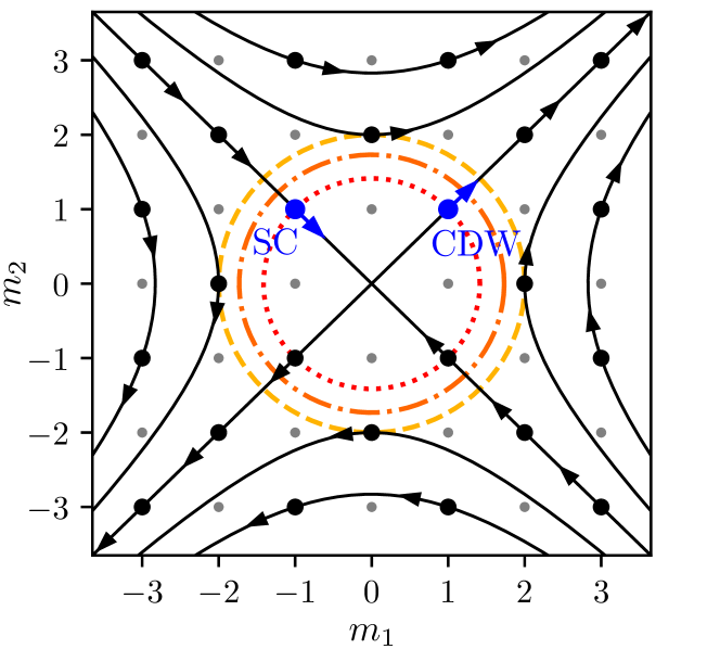
Figure 1: Lattice of perturbations for an $N=1$ channel LL. Large dots are bosonic operators, while small gray dots are fermionic ones; the latter can be ignored. A perturbation is relevant if it falls within the appropriate circle ( [0.4ex][x]20pt1.2pt4pt 1.5pt global, [0.4ex][x]22pt1.2pt6pt 1.5pt 1.2pt 1.5pt random, [0.4ex][x]19pt1.2pt1.2pt 1.5pt local). The lattice shown is $\mathbb{Z}^{2}$, corresponding to the noninteracting fixed point, $\lambda=0$. With attractive interactions, $\lambda<0$, the lattice deforms as indicated by the flow field. With repulsive interactions, $\lambda>0$, the flow is in the opposite direction.

Figure 1 illustrates these ideas in the simplest case, that of $N=1$ channel. The matrix $A\in SO(1,1)$ then describes a boost (hyperbolic rotation) of the plane, and can be parameterized as $A(\lambda)=e^{-(\lambda/2)\sigma_{x}}$. At the noninteracting fixed point, $\lambda=0$, the most relevant perturbations couple $\mathcal{O}_{\text{SC}}\equiv\psi^{\dagger}_{R}\psi^{\dagger}_{L}\sim e^{i(-\phi_{1}+\phi_{2})}$ to an external 3D superconductor, or $\mathcal{O}_{\text{CDW}}\equiv\psi^{\phantom{\dagger}}_{R}\psi^{\dagger}_{L}\sim e^{i(\phi_{1}+\phi_{2})}$ to a periodic potential. The corresponding lattice points are $\mathbf{m}=(-1,1)$ and $\mathbf{m}=(1,1)$ respectively. When $\lambda=0$, both operators have $\Delta=1$, so both perturbations are relevant; the associated instabilities are induced superconductivity (SC) and a pinned charge density wave (CDW) respectively. When interactions are turned on, so that $\lambda\neq 0$, the lattice deforms to $A(\lambda)\mathbb{Z}^{2}$ as indicated in the Figure. Thus, $\lambda<0$ makes $\mathcal{O}_{\text{CDW}}$ less relevant but $\mathcal{O}_{\text{SC}}$ more relevant, while $\lambda>0$ does the opposite. The interaction matrix $V$ can be parametrized as in Eq. (S13), with $X=u_{1}>0$, $Y=u_{2}>0$, and $M^{1/2}=A(-\lambda)=e^{(\lambda/2)\sigma_{x}}$; its off-diagonal element is $V_{12}=\frac{1}{2}(u_{1}+u_{2})\sinh{\lambda}$. Thus, $\lambda<0$ ($\lambda>0$) corresponds to attractive (repulsive) interactions, and we reproduce the well-known phenomenology of the 1-channel Luttinger liquid Giamarchi (2003). Clearly, stability is impossible with just $N=1$ channel.

Stable Luttinger Liquids. We now turn to the general case of $N$ channels. Our approach is to study all possible scaling dimension matrices $M$. After we have identified some $M$’s of interest, we reconstruct the corresponding $V$’s using Eq. (S13).

A useful structure theorem for $SO(N,N)$, called the hyperbolic cosine-sine (CS) decomposition Higham (2003), ensures that $M$ can be written as a product of independent boosts in orthogonal planes:

$$M=\begin{bmatrix}Q_{1}^{T}&0\\ 0&Q_{2}^{T}\end{bmatrix}\begin{bmatrix}C&-S\\ -S&C\end{bmatrix}\begin{bmatrix}Q_{1}&0\\ 0&Q_{2}\end{bmatrix},$$ (7)

where $Q_{1},Q_{2}\in SO(N)$, $C=\text{diag}(\cosh{\lambda_{i}})$, and $S=\text{diag}(\sinh{\lambda_{i}})$, with $\lambda_{i}\in\mathbb{R}$, $i=1,2,\dots,N$.

The crucial geometric fact distinguishing $N\geq 2$ from $N=1$ is that the boost planes of $M$ can be rotated out of alignment with the lattice planes of $\mathbb{Z}^{2N}$ by suitably chosen $Q_{i}$. As a consequence, for $N\geq 2$, absolutely $q$-stable phases exist for any finite $q$. This assertion can be proven quite simply, as follows.

Take $\lambda_{i}=\lambda$ in expression (7) for $M$, and let $\mathbf{m}=(\mathbf{m}_{R},\mathbf{m}_{L})$, with $\mathbf{m}_{R/L}\in\mathbb{Z}^{N}$. If either $\mathbf{m}_{R}$ or $\mathbf{m}_{L}$ vanishes, then $\Delta(\mathbf{m})=\frac{1}{2}\lVert\mathbf{m}\rVert^{2}\cosh{\lambda}>2$ for $\lambda>\mathrm{arccosh}\,2$. If neither $\mathbf{m}_{R}$ nor $\mathbf{m}_{L}$ vanishes, we can rewrite the inequality $\Delta(\mathbf{m})>2$ as

$$\lvert\hat{\mathbf{m}}_{R}^{T}Q\hat{\mathbf{m}}_{L}\rvert<f\Big{(}\frac{\lVert\mathbf{m}_{R}\rVert}{\lVert\mathbf{m}_{L}\rVert}\Big{)}\coth{\lambda}-\frac{2\operatorname{csch}{\lambda}}{\lVert\mathbf{m}_{R}\rVert\lVert\mathbf{m}_{L}\rVert},$$ (8)

where $Q\equiv Q_{1}^{T}Q_{2}\in SO(N)$, $\mathbf{\hat{m}}_{\nu}\equiv\mathbf{m}_{\nu}/\lVert\mathbf{m}_{\nu}\rVert$ and $f(x)\equiv\frac{1}{2}(x+x^{-1})$. There are a finite number of vectors $\mathbf{m}\in\mathbb{Z}^{2N}$ that satisfy $\lvert\mathbf{m}\rvert\leq q$, so the unit vectors $\mathbf{\hat{m}}_{R/L}$ in Eq. (8) belong to a finite set $\Omega_{q}$. This set cannot fill the unit sphere densely, so there exists $Q\in SO(N)$ and $\epsilon>0$ such that $\left\lvert\mathbf{\hat{m}}_{R}^{T}Q\hskip 1.0pt\mathbf{\hat{m}}_{L}\right\rvert<1-\epsilon$ for all $\mathbf{\hat{m}}_{R/L}\in\Omega_{q}$. But $f(x)\coth{\lambda}>1$ for any $x,\lambda>0$, while $\operatorname{csch}{\lambda}\to 0$ as $\lambda\to\infty$. Thus the right side of Eq. (8) is greater than $1-\epsilon$ for sufficiently large $\lambda$. ∎

In the $N=2$ channel case, $M$ is parameterized, according to Eq. (7), by two rapidities ($\lambda_{1},\lambda_{2}$) and two angles ($\theta_{1},\theta_{2}$, where $\theta_{i}$ is the rotation angle of $Q_{i}\in SO(2)$). It is convenient to write these as

$$\lambda_{1,2}=\delta\pm\lambda,\qquad\theta_{1,2}=\tfrac{1}{2}(\theta\mp\alpha).$$ (9)

In the limit $\delta\to 0$, the dependence on $\alpha$ disappears. The full parameterization of $M$ is written down explicitly in the Supplemental Material Sup .

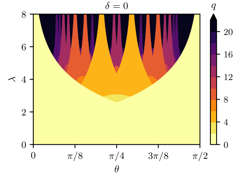
Figure 2: A slice of the absolute $q$-stability phase diagram for the $N=2$ channel LL. Each point on the plot is assigned the largest integer $q$ such that all perturbations with $\lvert\mathbf{m}\rvert\leq q$ are irrelevant for those parameter values $(\lambda,\theta)$. The diagram is identical for $\theta\mapsto\theta+n\pi/2$.

We construct an “absolute $q$-stability phase diagram” for the $2$-channel LL by assigning to each point $(\lambda,\delta,\theta,\alpha)$ in the resulting parameter space its absolute $q$-stability value, $q$. Figure 2 shows the $\delta=0$ slice of this diagram; other slices may be found in Ref. Sup . Each point in the phase diagram corresponds to a 6-parameter family of interaction matrices $V$, which can be obtained using Eq. (S13). The resulting general expression for $V$ is given in Ref. Sup . Here, we concentrate on the particular case in which the diagonal blocks $V_{RR}$ and $V_{LL}$ are equal, and $\delta=0$. In this case,

$$V=\left[\begin{array}[]{cc|cc}v_{+}&w&c_{+}&c_{0}\\ w&v_{-}&c_{0}&c_{-}\\[1.49994pt] \hline\cr c_{+}&c_{0}&v_{+}&w\\[-1.49994pt] c_{0}&c_{-}&w&v_{-}\end{array}\right],$$ (10)

where $v_{\pm}=v\pm u$,

$$c_{\pm} =(w\sin{\theta}\pm v_{\pm}\cos{\theta})\tanh{\lambda},$$ (11a)

$$c_{0} =v\sin{\theta}\tanh{\lambda}.$$ (11b)

The parameters $v$, $u$, and $w$ do not affect scaling dimensions; they can be chosen arbitrarily subject only to the constraint that $V$ must be positive definite, which requires $v>0$ and

$$(u\sin{\theta}-w\cos{\theta})^{2}\cosh^{2}\!\lambda+(u\cos{\theta}+w\sin{\theta})^{2}<v^{2}.$$ (12)

If in addition $\theta\in[0,\pi]$ and $u\cos{\theta}+w\sin{\theta}\geq v\lvert\cos{\theta}\rvert$, then every entry in the $V$ matrix is nonnegative. Note that the above inequalities can be satisfied simultaneously—the first defines the interior of an ellipse in the $(u/v,w/v)$ plane, and the second selects a segment of this ellipse. Thus, we can realize any of the absolutely $q$-stable phases in Figure 2 with purely repulsive interactions.

The 2-channel LLs defined by Eqs. (2) and (10–12) can in principle be realized in a single-spinful-channel quantum wire with either time-reversal or spatial inversion symmetry, but not both Sup . (We emphasize that these LL phases are $q$-stable with respect to perturbations that break the symmetry as well.) If the system also has spin-rotation symmetry about some axis, one can reformulate the effective action in terms of non-chiral charge and spin fields Giamarchi (2003); Sup . In the time-reversal invariant case, the corresponding Hamiltonian takes the form

$$H=\frac{1}{2\pi}\int dx\,\bigg{[} v_{c}K_{c}(\pi\Pi_{c})^{2}+\frac{v_{c}}{K_{c}}(\partial_{x}\varphi_{c})^{2}$$

$$+v_{s}K_{s}(\pi\Pi_{s})^{2}+\frac{v_{s}}{K_{s}}(\partial_{x}\varphi_{s})^{2}$$

$$+d_{+}(\pi\Pi_{c})\partial_{x}\varphi_{s}+d_{-}(\pi\Pi_{s})\partial_{x}\varphi_{c}\bigg{]},$$ (13)

where $\varphi_{c(s)}$ is the charge (spin) phase field, with conjugate momentum density $\Pi_{c(s)}$. The parameters $v_{c(s)},K_{c(s)},d_{\pm}$ are simple functions of $v_{\pm},w,c_{\pm},c_{0}$; the expressions are given in Ref. Sup . The $q$-stable phases identified in this work require $d_{+}\neq d_{-}$. Standard treatments of a spin-orbit-coupled LL, such as Ref. Moroz et al. (2000), make the additional assumption that interactions are pointlike; this leads to Eq. (Almost Perfect Metals in One Dimension) with $d_{+}=d_{-}$. However, $d_{+}\neq d_{-}$ is perfectly consistent with the symmetries of the problem, and appears naturally if one allows for more general short-range interactions.

Conclusions. As we have seen in this paper, the 1-channel Luttinger liquid is the exception. For any number of channels $N>1$—including even $N=2$—there are parameter regimes in which, for any desired finite $q$, all instabilities up to $q$-th order in electron operators are kept at bay. These phases are, in some sense, better examples of non-Fermi liquids than the 1-channel LL since they do not have a tendency to order frustrated only by low dimension. We cannot take $q=\infty$, so these states will eventually be unstable, but this may not occur until unobservably low temperatures. Moreover, it is much more likely that it will be possible to tune the parameters of an $N=2$ channel Luttinger liquid into the necessary regime in an experiment than it would be for $N=23$, which appears to be necessary for $q=\infty$. Thus, the work in this paper may facilitate the observation of these phases in experiments and may serve as a useful paradigm for thinking about higher-dimensional non-Fermi liquids. Our results can also be translated into statements about stable phases of classical 2-dimensional or layered 3-dimensional systems; it would be interesting to explore the consequences for particular classical systems of experimental interest.

S1 Restrictions on the interaction matrix $V$ imposed by symmetries

Consider the effective theory of a system that is invariant under one or more symmetries that interchange right and left-movers, such as time-reversal ($\mathcal{T}$), and/or spatial inversion ($\mathcal{P}$). On general grounds, $\mathcal{T}$ must be implemented in the effective theory by an anti-unitary operator that squares to $-1$ when acting on fermionic operators. Spatial inversion $\mathcal{P}$ must be implemented by a unitary operator that squares to $+1$.

S1.1 $\mathcal{T}$ symmetry but no $\mathcal{P}$ symmetry

First consider the case in which the system has time-reversal symmetry but no inversion symmetry. The chiral boson fields $\phi_{I}$ can be chosen to transform as follows under time-reversal (here the index $I=1,2,\dots N$):

$$\mathcal{T}:\begin{cases}\phi_{I}(x,t)&\longrightarrow\quad\phi_{I+N}(x,-t),\\ \phi_{I+N}(x,t)&\longrightarrow\quad\pi+\phi_{I}(x,-t).\end{cases}$$ (S1)

In addition, $\mathcal{T}$ complex conjugates $i\to-i$. Then, $\mathcal{T}$ correctly interchanges right- and left-movers, and squares to $-1$ when acting on the fermion fields $\psi_{I}\propto e^{\mp i\phi_{I}}\gamma_{I}$. (Alternatively, one could omit the $\pi$ in Eq. (S1) and have the Klein factors $\gamma_{I}$ transform nontrivially.) In this representation, $\mathcal{T}$ symmetry imposes that the interaction matrix $V$ must satisfy

$$\Sigma V\Sigma=V,$$ (S2)

where $\Sigma\equiv\sigma_{x}\otimes\mathbb{I}_{N}$ and $\sigma_{x}$ is the usual Pauli matrix. Thus, $V$ must have the block form

$$V=\begin{bmatrix}V_{1}&V_{2}\\ V_{2}&V_{1}\end{bmatrix},$$ (S3)

where $V_{i}=V_{i}^{T}$. Conversely, any $2N\times 2N$ positive definite matrix $V$ of this form can serve as the interaction matrix of a $\mathcal{T}$-symmetric $N$-channel Luttinger liquid.

S1.2 $\mathcal{P}$ symmetry but no $\mathcal{T}$ symmetry

Next consider the case in which the system has inversion symmetry but no time-reversal symmetry. The chiral boson fields $\phi_{I}$ can be chosen to transform as follows under spatial inversion (again the index $I=1,2,\dots N$):

$$\mathcal{P}:\begin{cases}\phi_{I}(x,t)&\longrightarrow\quad-\phi_{I+N}(-x,t),\\ \phi_{I+N}(x,t)&\longrightarrow\quad-\phi_{I}(-x,t).\end{cases}$$ (S4)

Then, $\mathcal{P}$ correctly interchanges right- and left-movers, and squares to $+1$ when acting on the fermion fields $\psi_{I}$. In this representation, $\mathcal{P}$ symmetry imposes that the interaction matrix $V$ must satisfy Eq. (S2), and hence that it must have the block form (S3). Conversely, any $2N\times 2N$ positive definite matrix $V$ of the form (S3) can serve as the interaction matrix of a $\mathcal{P}$-symmetric $N$-channel Luttinger liquid.

S1.3 Both $\mathcal{T}$ and $\mathcal{P}$ symmetry

Finally, consider the case in which the system has both time-reversal symmetry and inversion symmetry. The transformation laws (S1) and (S4) correspond to different representations of the fermion fields in terms of bosons, and hence cannot be used simultaneously. As is well known, symmetry with respect to $\mathcal{P}\mathcal{T}$ enforces a twofold degeneracy of the bands at each point in $k$-space. Therefore, the low-energy effective theory now involves $4N$ chiral spinless Dirac fermions $\psi_{I}$, where $I=1,2,\dots,2N$ labels right-movers and $I=2N+1,\dots,4N$ labels left-movers. The corresponding chiral boson fields $\phi_{I}$ can be chosen to transform as follows under time-reversal and spatial inversion (here the index $I=1,2,\dots N$):

$$\mathcal{T}: \begin{cases}\phi_{I}(x,t)&\longrightarrow\quad\phi_{I+2N}(x,-t),\\ \phi_{I+N}(x,t)&\longrightarrow\quad\phi_{I+3N}(x,-t),\\ \phi_{I+2N}(x,t)&\longrightarrow\quad\pi+\phi_{I}(x,-t),\\ \phi_{I+3N}(x,t)&\longrightarrow\quad\pi+\phi_{I+N}(x,-t),\end{cases}$$ (S5a)

$$\mathcal{P}: \begin{cases}\phi_{I}(x,t)&\longrightarrow\quad-\phi_{I+3N}(-x,t),\\ \phi_{I+N}(x,t)&\longrightarrow\quad-\phi_{I+2N}(-x,t),\\ \phi_{I+2N}(x,t)&\longrightarrow\quad-\phi_{I+N}(-x,t),\\ \phi_{I+3N}(x,t)&\longrightarrow\quad-\phi_{I}(-x,t).\end{cases}$$ (S5b)

Now, $\mathcal{T}$ symmetry and $\mathcal{P}$ symmetry respectively impose that the interaction matrix $V$ must satisfy

$$(\mathcal{T})\qquad\Sigma_{1}V\Sigma_{1} =V,$$ (S6a)

$$(\mathcal{P})\qquad\Sigma_{2}V\Sigma_{2} =V,$$ (S6b)

where $\Sigma_{1}\equiv\sigma_{x}\otimes\mathbb{I}_{2}\otimes\mathbb{I}_{N}$ and $\Sigma_{2}\equiv\sigma_{x}\otimes\sigma_{x}\otimes\mathbb{I}_{N}$. Thus, $V$ must have the block form

$$V=\begin{bmatrix}V_{1}&V_{2}&V_{3}&V_{4}\\ V_{2}&V_{1}&V_{4}&V_{3}\\ V_{3}&V_{4}&V_{1}&V_{2}\\ V_{4}&V_{3}&V_{2}&V_{1}\end{bmatrix},$$ (S7)

where $V_{i}=V_{i}^{T}$. Conversely, any $4N\times 4N$ positive definite matrix $V$ of this form can serve as the interaction matrix of a $\mathcal{T}$- and $\mathcal{P}$-symmetric $2N$-channel Luttinger liquid.

S2 Properties of the map $\varphi:V\mapsto M$ from interaction matrices to scaling dimension matrices

Let $\mathscr{P}_{N}$ denote the set of real symmetric positive definite $N\times N$ matrices, and let $\mathscr{M}_{N}\equiv SO(N,N)\cap\mathscr{P}_{2N}$. The map $\varphi$ from interaction matrices $V\in\mathscr{P}_{2N}$ to “scaling dimension matrices” $M\in\mathscr{M}_{N}$ is defined as

$$\varphi :\mathscr{P}_{2N}\to\mathscr{M}_{N},$$ (S8)

$$\varphi :V\mapsto A^{T}\!A,$$

where $A\in SO(N,N)$ and $AV\!A^{T}=D$ is diagonal.

S2.1 General properties

The first and second lemmas below show that $\varphi$ is well-defined. The third, fourth and fifth lemmas characterize the inverse images $\varphi^{-1}(M)$, and yield the parameterization of $V$ matrices used in the main text. All of these results are elementary, but we record them here for completeness.

Lemma 1.

If $V\in\mathscr{P}_{2N}$, then there exists $A\in SO(N,N)$ such that $AV\!A^{T}=D$ is diagonal.

Proof.

(by construction). Let $V^{1/2}$ denote the unique symmetric positive definite square root of $V$, so that

$$V^{1/2}=(V^{1/2})^{T},\qquad V^{1/2}>0,\qquad(V^{1/2})^{2}=V,$$ (S9)

and let $V^{-1/2}\equiv(V^{1/2})^{-1}=(V^{-1})^{1/2}$. The matrix $V^{-1/2}KV^{-1/2}$ (where $K=-\mathbb{I}_{N}\oplus\mathbb{I}_{N}$) is symmetric, and can therefore be diagonalized by some $Q\in SO(2N)$. Furthermore, Sylvester’s theorem of inertia [S1] ensures that $V^{-1/2}KV^{-1/2}$ has $N$ positive and $N$ negative eigenvalues. Thus, $Q$ can be chosen so that

$$QV^{-1/2}KV^{-1/2}Q^{T}=D^{-1}K,$$ (S10)

where $D$ is diagonal and positive definite (this can be arranged by re-ordering the rows of $Q$ and, if necessary, multiplying one row by $-1$ to maintain $\det Q=+1$). Taking the determinant of both sides of Eq. (S10), we have $\det V=\det D$. Therefore $A\equiv D^{1/2}QV^{-1/2}$ satisfies the desired properties: $AKA^{T}=K$, $\det A=1$, and $AV\!A^{T}=D$. ∎

Lemma 2.

If $A_{i}\in SO(N,N)$ and $A_{i}V\!A_{i}^{T}=D_{i}$ is diagonal for $i=1,2$, then $A_{1}^{T}A_{1}=A_{2}^{T}A_{2}$.

Proof.

Note that every $A\in SO(N,N)$ is invertible, with $A^{-1}=KA^{T}K$, where $K=-\mathbb{I}_{N}\oplus\mathbb{I}_{N}$ (this follows immediately from the defining condition for the group, $AKA^{T}=K$, and the fact that $K^{2}=\mathbb{I}_{2N}$.). Thus, to prove the lemma it suffices to prove the equivalent statement that $D_{2}=AD_{1}A^{T}$ implies $A^{T}\!A=\mathbb{I}_{2N}$, where $A\equiv A_{2}A_{1}^{-1}\in SO(N,N)$.

Using $A^{T}=KA^{-1}K$, the equation $D_{2}=AD_{1}A^{T}$ can be rewritten as

$$D_{2}K=A(D_{1}K)A^{-1}.$$ (S11)

Thus, the matrices $D_{2}K$ and $D_{1}K$ are similar. But similar diagonal matrices can differ only by a permutation of the diagonal elements. Taking account of the sign structure due to $K$, one must have $D_{2}=PD_{1}P^{-1}$, with $P=P^{(1)}\oplus P^{(2)}$, where the $P^{(i)}$ are $N\times N$ permutation matrices. Defining $B\equiv P^{-1}\!A$, Eq. (S11) reduces to

$$D_{1}K=B(D_{1}K)B^{-1}.$$ (S12)

This implies that $B$ preserves each eigenspace of $D_{1}K$. Hence it must (at the very least) have the block form $B=B^{(1)}\oplus B^{(2)}$, where the $B^{(i)}$ are $N\times N$ matrices. Since $A=PB$, and $P$ has a similar block structure, one must also have $A=A^{(1)}\oplus A^{(2)}$, where the $A^{(i)}$ are $N\times N$ matrices. Then the condition $AKA^{T}=K$ implies $A^{(i)}\in O(N)$, so that $A^{T}\!A=\mathbb{I}_{2N}$. ∎

Lemma 3.

$V\in\varphi^{-1}(M)$ if and only if

$$V=M^{-1/2}\begin{bmatrix}X&0\\ 0&Y\end{bmatrix}M^{-1/2}$$ (S13)

for some $X,Y\in\mathscr{P}_{N}$, where $M^{-1/2}$ denotes the unique positive definite square root of $M^{-1}$.

Proof.

$(\Longrightarrow)$: Assume that $\varphi(V)=M$. Every $M\in\mathscr{M}_{N}=SO(N,N)\cap\mathscr{P}_{2N}$ has a unique positive definite symmetric square root $M^{1/2}\in\mathscr{M}_{N}$. Furthermore, any matrix $A$ that satisfies $A^{T}\!A=M$ can be written as $A=RM^{1/2}$, for a suitable $R\in O(2N)$. If $A\in SO(N,N)$, then we must have $R\in O(2N)\cap SO(N,N)=O(N)\times O(N)/\mathbb{Z}_{2}$. Therefore, $\varphi(V)=M$ implies that $(RM^{1/2})V(RM^{1/2})^{T}=D$ for some diagonal positive definite $D$ and some $R\in O(N)\times O(N)/\mathbb{Z}_{2}$; equivalently, $V=M^{-1/2}R^{T}DRM^{-1/2}$, which is of the form indicated.

$(\Longleftarrow)$: Assume that $V$ has the form indicated. Then there exist $R_{1},R_{2}\in SO(N)$ that diagonalize $X,Y$ respectively. Let $A\equiv[R_{1}\oplus R_{2}]M^{1/2}$. Then $A\in SO(N,N)$, $AV\!A^{T}=D$ is diagonal, and $A^{T}\!A=M$. Thus $\varphi(V)=M$. ∎

The scaling dimension matrix $M\in\mathscr{M}_{N}$ can, by the hyperbolic CS decomposition, be written as [Eq. (7) of the main text]:

$$M=\begin{bmatrix}Q_{1}^{T}&0\\ 0&Q_{2}^{T}\end{bmatrix}\begin{bmatrix}C&-S\,\\ -S&C\end{bmatrix}\begin{bmatrix}Q_{1}&0\\ 0&Q_{2}\end{bmatrix},$$ (S14)

where $Q_{1},Q_{2}\in O(N)$, $C=\text{diag}(\cosh{\lambda_{i}})$, and $S=\text{diag}(\sinh{\lambda_{i}})$, with $\lambda_{i}\geq 0$, $i=1,2,\dots,N$. Note that we can equivalently take $Q_{1},Q_{2}\in SO(N)$ if we allow one of the $\lambda_{i}$’s to be negative, as done in the main text.

Lemma 4.

$V\in\varphi^{-1}(M)$ if and only if

$$V=\begin{bmatrix}X+F\,YF^{T}&XF+F\,Y\\ F^{T}\!X+YF^{T}&F^{T}\!XF+Y\end{bmatrix},$$ (S15)

for some $X,Y\in\mathscr{P}_{N}$, where

$$F\equiv Q_{1}^{T}\,\text{diag}(\tanh(\lambda_{i}/2))\,Q_{2}.$$ (S16)

Proof.

According to Lemma 3, $V\in\varphi^{-1}(M)$ iff $V=M^{-1/2}[\tilde{X}\oplus\tilde{Y}]M^{-1/2}$ for some $\tilde{X},\tilde{Y}\in\mathscr{P}_{N}$. From Eq. (S14), it follows that

$$M^{-1/2}=\begin{bmatrix}\tilde{C}_{1}&\tilde{S}\\ \tilde{S}^{T}&\tilde{C}_{2}\end{bmatrix},$$ (S17)

where $\tilde{C}_{\nu}=Q_{\nu}^{T}\,\text{diag}(\cosh(\lambda_{i}/2))\,Q_{\nu}$ ($\nu=1,2$) and $\tilde{S}=Q_{1}^{T}\,\text{diag}(\sinh(\lambda_{i}/2))\,Q_{2}$. Thus,

$$V=\begin{bmatrix}\tilde{C}_{1}\tilde{X}\tilde{C}_{1}+\tilde{S}\,\tilde{Y}\tilde{S}^{T}&\tilde{C}_{1}\tilde{X}\tilde{S}+\tilde{S}\,\tilde{Y}\tilde{C}_{2}\\ \tilde{S}^{T}\!\tilde{X}\tilde{C}_{1}+\tilde{C}_{2}\tilde{Y}\tilde{S}^{T}&\tilde{S}^{T}\!\tilde{X}\tilde{S}+\tilde{C}_{2}\tilde{Y}\tilde{C}_{2}\end{bmatrix}.$$ (S18)

Now define $X\equiv\tilde{C}_{1}\tilde{X}\tilde{C}_{1}$ and $Y\equiv\tilde{C}_{2}\tilde{Y}\tilde{C}_{2}$. These maps from $\tilde{X},\tilde{Y}\in\mathscr{P}_{N}$ to $X,Y\in\mathscr{P}_{N}$ are bijections, because $\tilde{C}_{\nu}\in\mathscr{P}_{N}$. Noting that $\tilde{S}\tilde{C}_{2}^{-1}=\tilde{C}_{1}^{-1}\tilde{S}=F$, we obtain the claimed result, Eq. (S15). ∎

We now write the interaction matrix in block form as

$$V=\begin{bmatrix}V_{RR}&V_{RL}\\ V_{LR}&V_{LL}\end{bmatrix},$$ (S19)

where $V_{RR},V_{LL}\in\mathscr{P}_{N}$ and $V_{LR}=V_{RL}^{T}$.

Lemma 5.

$V\in\varphi^{-1}(M)$ if and only if

$$V_{RR} \in\mathscr{P}_{N},$$ (S20a)

$$V_{RR}-V_{RL}\,V_{LL}^{-1}\,V_{RL}^{T} \in\mathscr{P}_{N},$$ (S20b)

$$V_{RL}+F\,V_{RL}^{T}F-V_{RR}F-FV_{LL} =0,$$ (S20c)

where $F$ is defined in Eq. (S16) above.

Proof.

Equations (S20a) and (S20b) are the Schur complement condition for positive definiteness of a symmetric matrix [S2]; $V\in\mathscr{P}_{2N}$ iff these equations hold. By Lemma 3, $V\in\varphi^{-1}(M)$ iff $M^{1/2}VM^{1/2}=\tilde{X}\oplus\tilde{Y}$ for some $\tilde{X},\tilde{Y}\in\mathscr{P}_{N}$. In the notation of Eq. (S17), one has

$$M^{1/2}=\begin{bmatrix}\tilde{C}_{1}&-\tilde{S}\,\\ -\tilde{S}^{T}&\tilde{C}_{2}\end{bmatrix}.$$ (S21)

Conjugating the equation $M^{1/2}VM^{1/2}=\tilde{X}\oplus\tilde{Y}$ by the positive definite matrix $\tilde{C}_{1}^{-1}\oplus\tilde{C}_{2}^{-1}$, it becomes

$$\begin{bmatrix}\mathbb{I}_{N}&\!-F\\ -F^{T}&\!\mathbb{I}_{N}\end{bmatrix}\!\begin{bmatrix}V_{RR}&V_{RL}\\ V_{RL}^{T}&V_{LL}\end{bmatrix}\!\begin{bmatrix}\mathbb{I}_{N}&\!-F\\ -F^{T}&\!\mathbb{I}_{N}\end{bmatrix}=\begin{bmatrix}X&0\\ 0&Y\end{bmatrix},$$ (S22)

where $X\equiv\tilde{C}_{1}^{-1}\tilde{X}\tilde{C}_{1}^{-1}$ and $Y\equiv\tilde{C}_{2}^{-1}\tilde{Y}\tilde{C}_{2}^{-1}$. These maps from $\tilde{X},\tilde{Y}\in\mathscr{P}_{N}$ to $X,Y\in\mathscr{P}_{N}$ are bijections. Therefore, $V\in\varphi^{-1}(M)$ iff Eq. (S22) holds for some $X,Y\in\mathscr{P}_{N}$. The off-diagonal block of Eq. (S22) yields Eq. (S20c). The diagonal blocks of Eq. (S22) are automatically satisfied, because the matrix on the left side is positive definite (it was constructed by conjugating $V\in\mathscr{P}_{2N}$ by other matrices in $\mathscr{P}_{2N}$). ∎

S2.2 Restrictions on the scaling dimension matrix $M$ imposed by symmetries

Let $P$ be any permutation matrix that satisfies $P^{2}=\mathbb{I}_{2N}$ and $PKP=-K$. Let $\mathscr{S}_{P}\equiv\{A\in\mathbb{R}^{2N\times 2N}\mid PAP=A\}$. Then, the following results hold:

Lemma 6.

If $V\in\mathscr{P}_{2N}\cap\mathscr{S}_{P}$ and $M=\varphi(V)$, then $M\in\mathscr{S}_{P}$.

Proof.

Pick some $A\in SO(N,N)$ such that $AV\!A^{T}=D$ is diagonal, and define $B\equiv PAP$. It is easy to check that $BKB^{T}=K$ and $\det B=1$, so $B\in SO(N,N)$. Also, $BV\!B^{T}=PDP$ is diagonal, since $P$ is a permutation matrix. Thus, $M=B^{T}\!B=PA^{T}\!A\,P=PMP$. ∎

Lemma 7.

Assume $M\in\mathscr{M}_{N}\cap\mathscr{S}_{P}$. Then $V\in\varphi^{-1}(M)\cap\mathscr{S}_{P}$ if and only if $V=M^{-1/2}ZM^{-1/2}$ for some $Z\in(\mathscr{P}_{N}\times\mathscr{P}_{N})\cap\mathscr{S}_{P}$.

Proof.

Lemma 3 implies that $V\in\varphi^{-1}(M)$ iff $V$ has the specified form with $Z\in\mathscr{P}_{N}\times\mathscr{P}_{N}$. Note that $PM^{\pm 1/2}=M^{\pm 1/2}P$. Thus $V$ and $Z$ are conjugates of one another by an invertible matrix that commutes with $P$. It follows that $PVP=V$ iff $PZP=Z$. ∎

Taking $Z=\mathbb{I}_{2N}$ shows that $\varphi^{-1}(M)\cap\mathscr{S}_{P}$ is nonempty for any $M\in\mathscr{M}_{N}\cap\mathscr{S}_{P}$. Thus, the set of interaction matrices $V$ that satisfy the constraint $PVP=V$ maps (under $\varphi$) onto the set of scaling dimension matrices $M$ that satisfy the constraint $PMP=M$. The constraints on $V$ derived in Section S1 are precisely of the form $PVP=V$ (with $P=\Sigma$, $\Sigma_{1}$ or $\Sigma_{2}$). Hence the allowed scaling dimension matrices $M$ for a system with time-reversal ($\mathcal{T}$) and/or spatial inversion ($\mathcal{P}$) symmetry may be characterized as follows.

S2.2.1 $\mathcal{T}$ symmetry or $\mathcal{P}$ symmetry, but not both

First consider the case in which the system has either time-reversal symmetry or inversion symmetry, but not both. We choose the $2N$ chiral bosons $\phi_{I}$ to transform according to Eq. (S1) in the former case, and according to Eq. (S4) in the latter. Then, in either case, the scaling dimension matrix must satisfy

$$\Sigma M\Sigma=M,$$ (S23)

where $\Sigma\equiv\sigma_{x}\otimes\mathbb{I}_{N}$ (with no further constraints). Imposing this constraint on the hyperbolic CS decomposition of $M$, Eq. (S14), yields the conditions

$$QCQ^{T}=C,$$ (S24a)

$$QSQ=S,$$ (S24b)

where $Q\equiv Q_{1}Q_{2}^{T}$. Assume, without loss of generality, that there are $m$ distinct rapidities $\lambda_{\alpha}$ with multiplicities $N_{\alpha}$ (satisfying $N_{1}+\cdots+N_{m}=N$), ordered so that $C=\cosh L$, $S=\sinh L$, and $L=\lambda_{1}\mathbb{I}_{N_{1}}\oplus\lambda_{2}\mathbb{I}_{N_{2}}\oplus\cdots\oplus\lambda_{m}\mathbb{I}_{N_{m}}$. Then the conditions above require that

$$Q=R_{1}\oplus R_{2}\oplus\cdots\oplus R_{m},$$ (S25)

where $R_{\alpha}\in O(N_{\alpha})$ and $R_{\alpha}=R_{\alpha}^{T}$ (i.e. each $R_{\alpha}$ is an $N_{\alpha}\times N_{\alpha}$ reflection matrix). In the special case in which all rapidities are equal, one has

$$M=\begin{bmatrix}\mathbb{I}_{N}\cosh{\lambda}&-R\sinh{\lambda}\\ -R\sinh{\lambda}&\mathbb{I}_{N}\cosh{\lambda}\end{bmatrix},$$ (S26)

where $R\in O(N)$ and $R=R^{T}$.

S2.2.2 Both $\mathcal{T}$ and $\mathcal{P}$ symmetry

In the case that the system has both time-reversal and inversion symmetry, we choose the $4N$ chiral bosons $\phi_{I}$ to transform according to Eq. (S5). Then, the scaling dimension matrix must satisfy

$$(\mathcal{T})\qquad\Sigma_{1}M\Sigma_{1} =M,$$ (S27a)

$$(\mathcal{P})\qquad\Sigma_{2}M\Sigma_{2} =M,$$ (S27b)

where $\Sigma_{1}\equiv\sigma_{x}\otimes\mathbb{I}_{2}\otimes\mathbb{I}_{N}$ and $\Sigma_{2}\equiv\sigma_{x}\otimes\sigma_{x}\otimes\mathbb{I}_{N}$ (with no further independent constraints). We can again impose these constraints on the hyperbolic CS decomposition of $M$, Eq. (S14), to obtain an explicit parameterization of all scaling dimension matrices that are consistent with both $\mathcal{T}$ and $\mathcal{P}$ symmetry. However, the general parameterization is somewhat cumbersome, so we will omit it. In the special case in which all rapidities are equal, one finds

$$M=\begin{bmatrix}\mathbb{I}_{2N}\cosh{\lambda}&-R\sinh{\lambda}\\ -R\sinh{\lambda}&\mathbb{I}_{2N}\cosh{\lambda}\end{bmatrix},$$ (S28)

where $R\in O(2N)$ has the block form

$$R=\begin{bmatrix}R_{1}&R_{2}\\ R_{2}&R_{1}\end{bmatrix},$$ (S29)

with $R_{i}=R_{i}^{T}$ (i.e. $R$ is a $2N\times 2N$ reflection matrix with this particular block form).

S2.3 Intuition for the parameterization of $V$, Eq. (S13)

To gain some intuition for the parametrization (S13) of $V$, first consider the limit $M=\mathbb{I}_{2N}$. Then the interactions encoded in $X$ simply mix the right-movers amongst themselves, leading to new modes with renormalized velocities, while $Y$ does the same with the left-movers. All scaling dimensions (being determined by $M$ alone) remain equal to their values at the free fixed point. Next consider a different limit, $X=Y=\mathbb{I}_{N}$. Now $V=M^{-1}$ is itself in $SO(N,N)$, and its inverse gives the scaling dimensions directly. To connect these two limits, consider the Euclidean space of all symmetric $N\times N$ matrices, $\mathbb{R}^{N(N+1)/2}$. The positive definite matrices occupy the interior of a convex cone $\mathscr{P}_{N}\subset\mathbb{R}^{N(N+1)/2}$. The space of interaction matrices is $\mathscr{V}=\mathscr{P}_{2N}$. According to Eq. (S13), $\mathscr{V}$ should be regarded as a bundle of lower-dimensional convex cones $\mathscr{P}_{N}\times\mathscr{P}_{N}$ (parameterized by $X,Y$) as fibers over the $N^{2}$-dimensional submanifold $\mathscr{M}_{N}\equiv SO(N,N)\cap\mathscr{P}_{2N}$ (parameterized by $M$). The scaling dimensions $\Delta(\mathbf{m})$, regarded as functions from $\mathscr{V}\to\mathbb{R}$, are then constant on each fiber. Each Luttinger liquid phase, defined in terms of its instabilities (or lack thereof), thus extends over the interior of a solid cone emanating from the vertex of $\mathscr{V}$.

S2.4 Illustration of parameterization for $N=1$ channel

The $N=1$ channel case again provides a nice illustration of these general ideas. The set $\mathscr{V}=\mathscr{P}_{2}$ consists of all $2\times 2$ matrices

$$V=\begin{bmatrix}\alpha+\beta&\gamma\\ \gamma&\alpha-\beta\end{bmatrix}$$ (S30)

with $(\alpha,\beta,\gamma)\in\mathbb{R}^{3}$ and $\alpha>(\beta^{2}+\gamma^{2})^{1/2}$. This is quite clearly the interior of a circular cone in $\mathbb{R}^{3}$. The parameterization (S13), with $M=e^{-\lambda\sigma_{x}}\in\mathscr{M}_{1}$, corresponds to

$$\alpha =\tfrac{1}{2}(x+y)\cosh{\lambda},$$ (S31a)

$$\beta =\tfrac{1}{2}(x-y),$$ (S31b)

$$\gamma =\tfrac{1}{2}(x+y)\sinh{\lambda},$$ (S31c)

where $x,y>0$. For fixed $\lambda$, the image of the resulting map $(x,y)\mapsto(\alpha,\beta,\gamma)$ is a slice of the cone $\mathscr{P}_{2}$, in a plane parallel to the $\beta$-axis and at an angle $\arctan(\tanh{\lambda})$ from the $\alpha$-axis. Each such slice is the interior of a cone in $\mathbb{R}^{2}$, with an opening angle that decreases with increasing $\lvert\lambda\rvert$. In terms of stability with respect to clean SC and CDW perturbations, $\mathscr{V}=\mathscr{P}_{2}$ splits into four regions: $\lambda<-\log 2$ ($\Delta_{\text{SC}}<2<\Delta_{\text{CDW}}$), $-\log 2<\lambda<0$ ($\Delta_{\text{SC}}<\Delta_{\text{CDW}}<2$), $0<\lambda<\log 2$ ($\Delta_{\text{CDW}}<\Delta_{\text{SC}}<2$), and $\lambda>\log 2$ ($\Delta_{\text{CDW}}<2<\Delta_{\text{SC}}$). These regions indeed take the form of solid cones emanating from the vertex of $\mathscr{P}_{2}$, as illustrated in Figure S1.

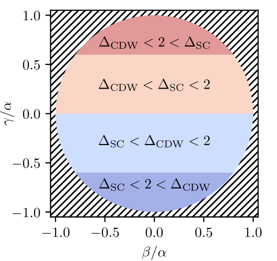
Figure S1: Phase diagram for the $N=1$ channel Luttinger liquid, in terms of stability with respect to global SC and CDW perturbations. The hatched region is unphysical ($V$ is not positive definite for these parameter values).

S3 Explicit parameterization of matrices for $N=2$ channel Luttinger liquid

S3.1 Scaling dimension matrix $M$

Let $Q(\phi)$ denote the $SO(2)$ rotation matrix

$$Q(\phi)\equiv\begin{bmatrix}\cos{\phi}&\sin{\phi}\\ -\sin{\phi}&\cos{\phi}\end{bmatrix},$$ (S32)

let $R(\phi)$ denote the $O(2)$ reflection matrix

$$R(\phi)\equiv\begin{bmatrix}\,\cos{\phi}&\sin{\phi}\\ \,\sin{\phi}&-\cos{\phi}\end{bmatrix},$$ (S33)

and let

$$L\equiv\begin{bmatrix}\delta+\lambda&0\\ 0&\delta-\lambda\end{bmatrix}.$$ (S34)

The parameterization of $M\in\mathscr{M}_{2}\equiv SO(2,2)\cap\mathscr{P}_{4}$ described in Eqs. (7) and (9) of the main text corresponds to

$$M=\begin{bmatrix}Q^{T}\!(\tfrac{\theta-\alpha}{2})&0\\ 0&Q^{T}\!(\tfrac{\theta+\alpha}{2})\end{bmatrix}\begin{bmatrix}\cosh{L}&-\sinh{L}\\ -\sinh{L}&\cosh{L}\end{bmatrix}\begin{bmatrix}Q(\tfrac{\theta-\alpha}{2})&0\\ 0&Q(\tfrac{\theta+\alpha}{2})\end{bmatrix},$$ (S35)

where each entry is a $2\times 2$ matrix. Performing the matrix multiplication, we can write the result as

$$M=\begin{bmatrix}\mathbb{I}_{2}\cosh{\lambda}&-R(\theta)\sinh{\lambda}\\ -R(\theta)\sinh{\lambda}&\mathbb{I}_{2}\cosh{\lambda}\end{bmatrix}\cosh{\delta}+\begin{bmatrix}R(\theta-\alpha)\sinh{\lambda}&-Q(\alpha)\cosh{\lambda}\\ -Q^{T}\!(\alpha)\cosh{\lambda}&R(\theta+\alpha)\sinh{\lambda}\end{bmatrix}\sinh{\delta},$$ (S36)

where $\mathbb{I}_{2}$ is the $2\times 2$ identity matrix. The dependence on $\alpha$ disappears in the limit $\delta\to 0$, as stated in the main text. Similarly, the dependence on $\theta$ disappears in the limit $\lambda\to 0$.

S3.1.1 $\mathcal{T}$ symmetry or $\mathcal{P}$ symmetry, but not both

If the system has either time-reversal symmetry or inversion symmetry, but not both, the scaling dimension matrix must satisfy $\Sigma M\Sigma=M$, where $\Sigma\equiv\sigma_{x}\otimes\mathbb{I}_{2}$. Applied to Eq. (S36), this condition requires $\alpha=0$. Hence, in this case,

$$M =\begin{bmatrix}Q^{T}\!(\theta/2)&0\\ 0&Q^{T}\!(\theta/2)\end{bmatrix}\begin{bmatrix}\cosh{L}&-\sinh{L}\\ -\sinh{L}&\cosh{L}\end{bmatrix}\begin{bmatrix}Q(\theta/2)&0\\ 0&Q(\theta/2)\end{bmatrix}$$ (S37a)

$$=\begin{bmatrix}\mathbb{I}_{2}\cosh{\lambda}&-R(\theta)\sinh{\lambda}\\ -R(\theta)\sinh{\lambda}&\mathbb{I}_{2}\cosh{\lambda}\end{bmatrix}\cosh{\delta}+\begin{bmatrix}R(\theta)\sinh{\lambda}&-\mathbb{I}_{2}\cosh{\lambda}\\ -\mathbb{I}_{2}\cosh{\lambda}&R(\theta)\sinh{\lambda}\end{bmatrix}\sinh{\delta}.$$ (S37b)

Note in particular that the presence of $\mathcal{T}$ symmetry or $\mathcal{P}$ symmetry (but not both simultaneously) places no restrictions on the allowed values of the parameters $\lambda$, $\delta$, and $\theta$. Changing the sign of $\lambda$ is equivalent to shifting $\theta$ by $\pi$, so we can assume $\lambda>0$.

S3.1.2 Both $\mathcal{T}$ and $\mathcal{P}$ symmetry

If the system has both time-reversal and inversion symmetry, the scaling dimension matrix must satisfy $\Sigma_{i}M\Sigma_{i}=M$ for $i=1,2$, where $\Sigma_{1}\equiv\sigma_{x}\otimes\mathbb{I}_{2}$ and $\Sigma_{2}\equiv\sigma_{x}\otimes\sigma_{x}$. Applied to Eq. (S36), these conditions require $\alpha=0$ and $\theta=\pi/2$. Hence, in this case,

$$M =\begin{bmatrix}Q^{T}\!(\pi/4)&0\\ 0&Q^{T}\!(\pi/4)\end{bmatrix}\begin{bmatrix}\cosh{L}&-\sinh{L}\\ -\sinh{L}&\cosh{L}\end{bmatrix}\begin{bmatrix}Q(\pi/4)&0\\ 0&Q(\pi/4)\end{bmatrix}$$ (S38a)

$$=\begin{bmatrix}\mathbb{I}_{2}\cosh{\lambda}&-\sigma_{x}\sinh{\lambda}\\ -\sigma_{x}\sinh{\lambda}&\mathbb{I}_{2}\cosh{\lambda}\end{bmatrix}\cosh{\delta}+\begin{bmatrix}\sigma_{x}\sinh{\lambda}&-\mathbb{I}_{2}\cosh{\lambda}\\ -\mathbb{I}_{2}\cosh{\lambda}&\sigma_{x}\sinh{\lambda}\end{bmatrix}\sinh{\delta}.$$ (S38b)

S3.2 Interaction matrix $V$ (general expressions)

We parameterize the interaction matrix $V\in\mathscr{P}_{4}$ using Lemma 4. Let

$$V=\begin{bmatrix}V_{RR}&V_{RL}\\ V_{RL}^{T}&V_{LL}\end{bmatrix}.$$ (S39)

Lemma 4 states that $V\in\varphi^{-1}(M)$ if and only if

$$V_{RR} =X+F\,YF^{T},$$ (S40a)

$$V_{LL} =Y+F^{T}\!XF,$$ (S40b)

$$V_{RL} =XF+F\,Y$$ (S40c)

for some $X,Y\in\mathscr{P}_{2}$. The $2\times 2$ matrix $F$ corresponding to the $M$ given in Eqs. (S35) or (S36) is

$$F=Q^{T}\!(\tfrac{\theta-\alpha}{2})\begin{bmatrix}\tanh(\tfrac{\delta+\lambda}{2})&0\\ 0&\tanh(\tfrac{\delta-\lambda}{2})\end{bmatrix}Q(\tfrac{\theta+\alpha}{2})=\frac{\sinh{\lambda}}{\cosh{\lambda}+\cosh{\delta}}\,R(\theta)+\frac{\sinh{\delta}}{\cosh{\lambda}+\cosh{\delta}}\,Q(\alpha),$$ (S41)

where $Q(\phi)$ and $R(\phi)$ are defined in Eqs. (S32) and (S33).

The matrices $X,Y\in\mathscr{P}_{2}$ can be conveniently parameterized as

$$X =\begin{bmatrix}x_{0}+x_{1}&x_{2}\\ x_{2}&x_{0}-x_{1}\end{bmatrix},$$ (S42a)

$$Y =\begin{bmatrix}y_{0}+y_{1}&\ y_{2}\\ y_{2}&\ y_{0}-y_{1}\end{bmatrix},$$ (S42b)

where $(x_{0},x_{1},x_{2})\in\mathbb{R}^{3}$, $x_{0}>(x_{1}^{2}+x_{2}^{2})^{1/2}$, and $(y_{0},y_{1},y_{2})\in\mathbb{R}^{3}$, $y_{0}>(y_{1}^{2}+y_{2}^{2})^{1/2}$. Using Eqs. (S41) and (S42) in Eq. (S40), we obtain

$$V_{RR} =\begin{bmatrix}x_{0}+x_{1}&x_{2}\\ x_{2}&x_{0}-x_{1}\end{bmatrix}+\frac{\sinh^{2}\!\lambda}{(\cosh{\lambda}+\cosh{\delta})^{2}}\begin{bmatrix}y_{0}+y_{1}\cos{2\theta}+y_{2}\sin{2\theta}&y_{1}\sin{2\theta}-y_{2}\cos{2\theta}\\ y_{1}\sin{2\theta}-y_{2}\cos{2\theta}&y_{0}-y_{1}\cos{2\theta}-y_{2}\sin{2\theta}\end{bmatrix}$$

$$\quad+\frac{2\sinh{\lambda}\sinh{\delta}}{(\cosh{\lambda}+\cosh{\delta})^{2}}\begin{bmatrix}y_{1}\cos(\theta+\alpha)+y_{2}\sin(\theta+\alpha)+y_{0}\cos(\theta-\alpha)&y_{0}\sin(\theta-\alpha)\\ y_{0}\sin(\theta-\alpha)&y_{1}\cos(\theta+\alpha)+y_{2}\sin(\theta+\alpha)-y_{0}\cos(\theta-\alpha)\end{bmatrix}$$

$$\quad+\frac{\sinh^{2}\!\delta}{(\cosh{\lambda}+\cosh{\delta})^{2}}\begin{bmatrix}y_{0}+y_{1}\cos{2\alpha}+y_{2}\sin{2\alpha}&y_{2}\cos{2\alpha}-y_{1}\sin{2\alpha}\\ y_{2}\cos{2\alpha}-y_{1}\sin{2\alpha}&y_{0}-y_{1}\cos{2\alpha}-y_{2}\sin{2\alpha}\end{bmatrix},$$ (S43a)

$$V_{LL} =\begin{bmatrix}y_{0}+y_{1}&y_{2}\\ y_{2}&y_{0}-y_{1}\end{bmatrix}+\frac{\sinh^{2}\!\lambda}{(\cosh{\lambda}+\cosh{\delta})^{2}}\begin{bmatrix}x_{0}+x_{1}\cos{2\theta}+x_{2}\sin{2\theta}&x_{1}\sin{2\theta}-x_{2}\cos{2\theta}\\ x_{1}\sin{2\theta}-x_{2}\cos{2\theta}&x_{0}-x_{1}\cos{2\theta}-x_{2}\sin{2\theta}\end{bmatrix}$$

$$\quad+\frac{2\sinh{\lambda}\sinh{\delta}}{(\cosh{\lambda}+\cosh{\delta})^{2}}\begin{bmatrix}x_{1}\cos(\theta-\alpha)+x_{2}\sin(\theta-\alpha)+x_{0}\cos(\theta+\alpha)&x_{0}\sin(\theta+\alpha)\\ x_{0}\sin(\theta+\alpha)&x_{1}\cos(\theta-\alpha)+x_{2}\sin(\theta-\alpha)-x_{0}\cos(\theta+\alpha)\end{bmatrix}$$

$$\quad+\frac{\sinh^{2}\!\delta}{(\cosh{\lambda}+\cosh{\delta})^{2}}\begin{bmatrix}x_{0}+x_{1}\cos{2\alpha}-x_{2}\sin{2\alpha}&x_{1}\sin{2\alpha}+x_{2}\cos{2\alpha}\\ x_{1}\sin{2\alpha}+x_{2}\cos{2\alpha}&x_{0}-x_{1}\cos{2\alpha}+x_{2}\sin{2\alpha}\end{bmatrix},$$ (S43b)

$$V_{RL} =\frac{\sinh{\lambda}}{\cosh{\lambda}+\cosh{\delta}}\begin{bmatrix}(x_{1}+y_{1}+x_{0}+y_{0})\cos{\theta}+(x_{2}+y_{2})\sin{\theta}&(x_{0}+y_{0}+x_{1}-y_{1})\sin{\theta}-(x_{2}-y_{2})\cos{\theta}\\ (x_{0}+y_{0}-x_{1}+y_{1})\sin{\theta}+(x_{2}-y_{2})\cos{\theta}&(x_{1}+y_{1}-x_{0}-y_{0})\cos{\theta}+(x_{2}+y_{2})\sin{\theta}\end{bmatrix}$$

$$\quad+\frac{\sinh{\delta}}{\cosh{\lambda}+\cosh{\delta}}\begin{bmatrix}(x_{0}+y_{0}+x_{1}+y_{1})\cos{\alpha}-(x_{2}-y_{2})\sin{\alpha}&(x_{2}+y_{2})\cos{\alpha}+(x_{1}-y_{1}+x_{0}+y_{0})\sin{\alpha}\\ (x_{2}+y_{2})\cos{\alpha}+(x_{1}-y_{1}-x_{0}-y_{0})\sin{\alpha}&(x_{0}+y_{0}-x_{1}-y_{1})\cos{\alpha}+(x_{2}-y_{2})\sin{\alpha}\end{bmatrix}.$$ (S43c)

Equation (S43) gives a complete and explicit parameterization of the possible interaction matrices $V\in\mathscr{P}_{4}$ of a $2$-channel Luttinger liquid, in terms of the ten real parameters $(\lambda,\delta,\theta,\alpha,x_{0},x_{1},x_{2},y_{0},y_{1},y_{2})$. Of these, only the first four $(\lambda,\delta,\theta,\alpha)$ affect scaling dimensions; they determine the scaling dimension matrix $M$ via Eq. (S36). The remaining six parameters can be chosen arbitrarily, subject only to the constraints $x_{0}>(x_{1}^{2}+x_{2}^{2})^{1/2}$ and $y_{0}>(y_{1}^{2}+y_{2}^{2})^{1/2}$ (if either of these inequalities is violated, the resulting $V$ will fail to be positive definite).

S3.2.1 $\mathcal{T}$ symmetry or $\mathcal{P}$ symmetry, but not both

When symmetries are present, it is convenient to parameterize the interaction matrix $V\in\mathscr{P}_{4}$ using Lemma 7 instead. In the present case, Lemma 7 gives $V=M^{-1/2}[X\oplus Y]M^{-1/2}$ with $X,Y\in\mathscr{P}_{2}$ satisfying $\Sigma[X\oplus Y]\Sigma=X\oplus Y$, where $\Sigma\equiv\sigma_{x}\otimes\mathbb{I}_{2}$; the condition fixes $Y=X$. Thus, $V=M^{-1/2}[X\oplus X]M^{-1/2}$ with $X\in\mathscr{P}_{2}$. The scaling dimension matrix $M$ is given by Eq. (S37). Thus,

$$M^{-1/2}=\begin{bmatrix}Q^{T}\!(\theta/2)&0\\ 0&Q^{T}\!(\theta/2)\end{bmatrix}\begin{bmatrix}\cosh(L/2)&\sinh(L/2)\\ \sinh(L/2)&\cosh(L/2)\end{bmatrix}\begin{bmatrix}Q(\theta/2)&0\\ 0&Q(\theta/2)\end{bmatrix}.$$ (S44)

The inner factors of $Q(\theta/2)$ in the product $V=M^{-1/2}[X\oplus X]M^{-1/2}$ may be absorbed into $X$, since the latter is an arbitrary element of $\mathscr{P}_{2}$. Doing so, we obtain

$$V=\begin{bmatrix}Q^{T}\!(\theta/2)&0\\ 0&Q^{T}\!(\theta/2)\end{bmatrix}\begin{bmatrix}\cosh(L/2)&\sinh(L/2)\\ \sinh(L/2)&\cosh(L/2)\end{bmatrix}\begin{bmatrix}X&0\\ 0&X\end{bmatrix}\begin{bmatrix}\cosh(L/2)&\sinh(L/2)\\ \sinh(L/2)&\cosh(L/2)\end{bmatrix}\begin{bmatrix}Q(\theta/2)&0\\ 0&Q(\theta/2)\end{bmatrix}.$$ (S45)

We can parameterize $X\in\mathscr{P}_{2}$ as

$$X=\zeta\begin{bmatrix}1+a&-b\\ -b&1-a\end{bmatrix},$$ (S46)

where $\zeta>0$ and $(a,b)\in\mathbb{R}^{2}$, $a^{2}+b^{2}<1$. Performing the matrix multiplications in Eq. (S45), we obtain

$$V=\zeta\begin{bmatrix}V_{1}&V_{2}\\ V_{2}&V_{1}\end{bmatrix}\cosh{\delta}+\zeta\begin{bmatrix}V_{2}&V_{1}\\ V_{1}&V_{2}\end{bmatrix}\sinh{\delta},$$ (S47)

where

$$V_{1} =\begin{bmatrix}\cosh{\lambda}+a\cos{\theta}\cosh{\lambda}+b\sin{\theta}&a\sin{\theta}\cosh{\lambda}-b\cos{\theta}\\ a\sin{\theta}\cosh{\lambda}-b\cos{\theta}&\cosh{\lambda}-a\cos{\theta}\cosh{\lambda}-b\sin{\theta}\end{bmatrix},$$ (S48a)

$$V_{2} =\begin{bmatrix}a+\cos{\theta}&\sin{\theta}\\ \sin{\theta}&a-\cos{\theta}\end{bmatrix}\sinh{\lambda}.$$ (S48b)

Equations (S47) and (S48) gives a complete and explicit parameterization of the possible interaction matrices $V\in\mathscr{P}_{4}$ of a $2$-channel Luttinger liquid with either time-reversal symmetry or inversion symmetry (but not both), in terms of the six real parameters $(\lambda,\delta,\theta,a,b,\zeta)$. Of these, only the first three $(\lambda,\delta,\theta)$ affect scaling dimensions; they determine the scaling dimension matrix $M$ via Eq. (S37). The remaining three parameters can be chosen arbitrarily, subject only to the constraints $a^{2}+b^{2}<1$ and $\zeta>0$ (if these inequalities are violated, the resulting $V$ will fail to be positive definite). Note that $\zeta$ is an irrelevant overall scale factor.

S3.2.2 Both $\mathcal{T}$ and $\mathcal{P}$ symmetry

As above, we parameterize the interaction matrix $V\in\mathscr{P}_{4}$ using Lemma 7. In this case, Lemma 7 gives $V=M^{-1/2}[X\oplus Y]M^{-1/2}$ with $X,Y\in\mathscr{P}_{2}$ satisfying $\Sigma_{i}[X\oplus Y]\Sigma_{i}=X\oplus Y$ for $i=1,2$, where $\Sigma_{1}\equiv\sigma_{x}\otimes\mathbb{I}_{2}$ and $\Sigma_{2}\equiv\sigma_{x}\otimes\sigma_{x}$. The conditions fix $Y=X=x_{0}\mathbb{I}_{2}+x_{1}\sigma_{x}$, with $(x_{0},x_{1})\in\mathbb{R}^{2}$, $x_{0}>\lvert x_{1}\rvert$. Thus, $V=M^{-1/2}[X\oplus X]M^{-1/2}$ with $X$ of the form specified. The scaling dimension matrix $M$ is given by Eq. (S38). Thus,

$$M^{-1/2}=\begin{bmatrix}Q^{T}\!(\pi/4)&0\\ 0&Q^{T}\!(\pi/4)\end{bmatrix}\begin{bmatrix}\cosh(L/2)&\sinh(L/2)\\ \sinh(L/2)&\cosh(L/2)\end{bmatrix}\begin{bmatrix}Q(\pi/4)&0\\ 0&Q(\pi/4)\end{bmatrix}.$$ (S49)

Writing $X=\zeta(\mathbb{I}_{2}+a\sigma_{x})$ with $\zeta>0$, $\lvert a\rvert<1$, and performing the matrix multiplications in $V=M^{-1/2}[X\oplus X]M^{-1/2}$, we obtain

$$V=\zeta\begin{bmatrix}V_{1}&V_{2}\\ V_{2}&V_{1}\end{bmatrix}\cosh{\delta}+\zeta\begin{bmatrix}V_{2}&V_{1}\\ V_{1}&V_{2}\end{bmatrix}\sinh{\delta},$$ (S50)

where

$$V_{1} =\begin{bmatrix}1&a\\ a&1\end{bmatrix}\cosh{\lambda},$$ (S51a)

$$V_{2} =\begin{bmatrix}a&1\\ 1&a\end{bmatrix}\sinh{\lambda}.$$ (S51b)

Equations (S50) and (S51) gives a complete and explicit parameterization of the possible interaction matrices $V\in\mathscr{P}_{4}$ of a $2$-channel Luttinger liquid with both time-reversal and inversion symmetry, in terms of the four real parameters $(\lambda,\delta,a,\zeta)$. Of these, only the first two $(\lambda,\delta)$ affect scaling dimensions; they determine the scaling dimension matrix $M$ via Eq. (S38). The remaining two parameters can be chosen arbitrarily, subject only to the constraints $\lvert a\rvert<1$ and $\zeta>0$ (if these inequalities are violated, the resulting $V$ will fail to be positive definite). Note that, as before, $\zeta$ is an irrelevant overall scale factor.

S3.3 Interaction matrix $V$ with $\mathcal{T}$ or $\mathcal{P}$ symmetry (but not both), in the special case $\delta=0$

In the limit $\delta\to 0$, Eqs. (S47) and (S48) together yield

$$V=\left[\begin{array}[]{cc|cc}v_{+}&\!w&c_{+}&c_{0}\\ w&v_{-}&c_{0}&c_{-}\\[1.49994pt] \hline\cr c_{+}&c_{0}&\,v_{+}&\!w\\[-1.49994pt] c_{0}&c_{-}&w&v_{-}\end{array}\right],$$ (S52)

where

$$v_{\pm} =v\pm u,$$ (S53a)

$$v =\zeta\cosh{\lambda},$$ (S53b)

$$u =\zeta(a\cos{\theta}\cosh{\lambda}+b\sin{\theta}),$$ (S53c)

$$w =\zeta(a\sin{\theta}\cosh{\lambda}-b\cos{\theta}),$$ (S53d)

$$c_{\pm} =\zeta(a\pm\cos{\theta})\sinh{\lambda},$$ (S53e)

$$c_{0} =\zeta\sin{\theta}\sinh{\lambda}.$$ (S53f)

We assume $\lambda>0$ (without loss of generality), and identify the values of $a,b$ for which all matrix elements of $V$ are nonnegative. The diagonal elements of a positive definite matrix are necessarily positive, so $v_{\pm}>0$ is automatic. $c_{0}\geq 0$ requires $\theta\in[0,\pi]$. Nonnegativity of the remaining matrix elements, $c_{\pm}$ and $w$, requires

$$a \geq\lvert\cos{\theta}\rvert,$$ (S54a)

$$a\sin{\theta}\cosh{\lambda} \geq b\cos{\theta}.$$ (S54b)

In fact, Eq. (S54b) is superfluous, because it follows from Eq. (S54a) and the positive definiteness condition $a^{2}+b^{2}<1$; assuming the latter, we have $\lvert b\rvert<(1-a^{2})^{1/2}\leq\lvert\sin{\theta}\rvert\leq\lvert\cos{\theta}\tan{\theta}\rvert\cosh{\lambda}\leq a\lvert\tan{\theta}\rvert\cosh{\lambda}$, which implies Eq. (S54b) if $\theta\in[0,\pi]$. We conclude that the $V$ matrix given above is positive definite with all entries nonnegative if $\lambda>0$, $\theta\in[0,\pi]$, $a^{2}+b^{2}<1$, and $a\geq\lvert\cos{\theta}\rvert$.

These results are completely equivalent to the ones stated in the main text. Indeed, using Eq. (S53), one can verify that the following linear relations hold:

$$c_{\pm} =(w\sin{\theta}\pm v_{\pm}\cos{\theta})\tanh{\lambda},$$ (S55a)

$$c_{0} =v\sin{\theta}\tanh{\lambda}.$$ (S55b)

These are precisely the relations that one obtains by using Eq. (S52) and $F=Q(\theta)\tanh(\lambda/2)$ in Eq. (S20c) of Lemma 5. Therefore, we can regard $(v,u,w)$, instead of $(\zeta,a,b)$, as the independent variables parameterizing $V$. From Eq. (S53), we have

$$\begin{bmatrix}u/v\\ w/v\end{bmatrix}=\begin{bmatrix}\cos{\theta}&\sin{\theta}\operatorname{sech}{\lambda}\\ \sin{\theta}&-\cos{\theta}\operatorname{sech}{\lambda}\end{bmatrix}\begin{bmatrix}a\\ b\end{bmatrix}.$$ (S56)

Inverting this linear system,

$$\begin{bmatrix}a\\ b\end{bmatrix}=\begin{bmatrix}\cos{\theta}&\sin{\theta}\\ \,\sin{\theta}\cosh{\lambda}&-\cos{\theta}\cosh{\lambda}\end{bmatrix}\begin{bmatrix}u/v\\ w/v\end{bmatrix}.$$ (S57)

Thus, the conditions $a^{2}+b^{2}<1$ and $a\geq\lvert\cos{\theta}\rvert$ translate to:

$$(u\sin{\theta}-w\cos{\theta})^{2}\cosh^{2}\!\lambda+(u\cos{\theta}+w\sin{\theta})^{2} <v^{2},$$ (S58a)

$$u\cos{\theta}+w\sin{\theta} \geq v\lvert\cos{\theta}\rvert.$$ (S58b)

These conditions are stated in the main text as Eq. (12) and the in-line equation just below it.

S4 Absolute $q$-stability phase diagram for $N=2$ channel Luttinger liquid

The interaction matrix $V\in\mathscr{P}_{4}$ of a $2$-channel Luttinger liquid depends on ten real parameters; these can be chosen according to Eq. (S43). Of the ten, only the four parameters $\xi\equiv(\lambda,\delta,\theta,\alpha)$ affect scaling dimensions; they determine the scaling dimension matrix $M(\xi)$ via Eq. (S36), which in turn determines $\Delta(\mathbf{m};\xi)\equiv\tfrac{1}{2}\mathbf{m}^{T}\!M(\xi)\mathbf{m}$.

Let $q(\xi)$ denote the absolute $q$-stability value of a Luttinger liquid with parameters $\xi$. By definition, $q(\xi)$ is the largest integer such that $\Delta(\mathbf{m};\xi)>2$ for all nonzero $\mathbf{m}\in\mathbb{Z}^{4}$ with $K(\mathbf{m})\in\mathbb{Z}$ and $\lvert\mathbf{m}\rvert\leq q(\xi)$, where $K(\mathbf{m})\equiv\tfrac{1}{2}\mathbf{m}^{T}\!K\mathbf{m}$, $K\equiv\mathbb{I}_{2}\oplus-\mathbb{I}_{2}$. Because of the inequality $\Delta(\mathbf{m})\geq\lvert K(\mathbf{m})\rvert$, one can restrict attention to those $\mathbf{m}$ for which $K(\mathbf{m})=0,\pm 1,\pm 2$. Thus, an equivalent definition of $q(\xi)$ to the one given above is: $q(\xi)$ is the smallest positive integer such that $\Delta(\mathbf{m};\xi)\leq 2$ for some $\mathbf{m}\in\mathbb{Z}^{4}$ with $K(\mathbf{m})\in\{0,\pm 1,\pm 2\}$ and $\lvert\mathbf{m}\rvert=q(\xi)+1$.

We use the second definition to determine the phase diagram numerically. The algorithm is straightforward: at each point $\xi$, compute $\Delta(\mathbf{m};\xi)$ for all integer vectors $\mathbf{m}$ with $K(\mathbf{m})\in\{0,\pm 1,\pm 2\}$ in shells of increasing $\lvert\mathbf{m}\rvert$, until either a vector $\mathbf{m}_{*}$ is found for which $\Delta(\mathbf{m}_{*};\xi)\leq 2$, or $\lvert\mathbf{m}\rvert$ passes a specified cutoff value $q_{*}$. Set $q(\xi)=\lvert\mathbf{m}_{*}\rvert-1$ in the former case, and $q(\xi)=q_{*}$ in the latter. The shells of vectors with $\lvert\mathbf{m}\rvert=2,\dots,q_{*}$ can be tabulated in advance, and the matrix $M(\xi)$ only needs to be computed once at each point $\xi$. Figure 2 of the main text and Figure S2 below were obtained by this method, with cutoff $q_{*}=22$.

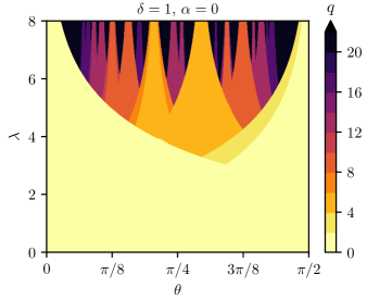
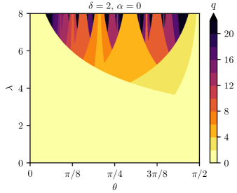
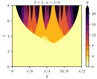
Figure S2: Various slices of the absolute $q$-stability phase diagram for the $N=2$ channel Luttinger liquid (compare Figure 2 of the main text).

S5 Representation of $2$-channel Luttinger liquid in terms of charge and spin fields

A single-spinful-channel quantum wire provides the simplest example of a $2$-channel Luttinger liquid. Standard treatments of this problem Giamarchi (2003) are usually phrased in terms of non-chiral charge ($c$) and spin ($s$) fields, $\varphi_{c}$ and $\varphi_{s}$, and their canonical conjugates, $\Pi_{c}\equiv\frac{1}{\pi}\partial_{x}\vartheta_{c}$ and $\Pi_{s}\equiv\frac{1}{\pi}\partial_{x}\vartheta_{s}$ respectively. These fields are related to the slowly varying parts of the charge density, $\rho_{c}$, and spin density, $\rho_{s}$, via $\rho_{c}=-\frac{1}{\pi}\partial_{x}\varphi_{c}$ and $\rho_{s}=-\frac{1}{\pi}\partial_{x}\varphi_{s}$ (we follow the normalization and sign conventions of Ref. Giamarchi (2003)). Our analysis, meanwhile, is phrased in terms of chiral boson fields $\phi_{I}$, which are related to the densities at each Fermi point via $\rho_{I}=\frac{1}{2\pi}\partial_{x}\phi_{I}$.

A rigorous reformulation of the bosonic effective theory in terms of charge and spin fields is possible when the system is invariant under spin rotations about some axis $\mathbf{\hat{n}}$. (Note that such a symmetry, by itself, imposes no constraints on the interaction matrix $V$.) Then, the component of the spin along $\mathbf{\hat{n}}$ is a good quantum number, and it labels the different Fermi points. One possibility for this labelling is

$$(\phi_{1},\phi_{2},\phi_{3},\phi_{4})=(\phi_{R\uparrow},\phi_{R\downarrow},\phi_{L\downarrow},\phi_{L\uparrow}),$$ (S59)

where $R/L$ distinguishes right movers from left movers, and $\uparrow/\downarrow$ denotes the spin component along $\mathbf{\hat{n}}$. With the choice (S59), the fields transform under time-reversal $\mathcal{T}$ according to Eq. (S1).

Another possibility is to take

$$(\phi_{1},\phi_{2},\phi_{3},\phi_{4})=(\phi_{R\uparrow},\phi_{R\downarrow},\phi_{L\uparrow},\phi_{L\downarrow}).$$ (S60)

With the choice (S60), the fields transform under spatial inversion $\mathcal{P}$ according to Eq. (S4).

In either case, one has

$$\begin{bmatrix}\varphi_{c}\\ \vartheta_{c}\\ \varphi_{s}\\ \vartheta_{s}\end{bmatrix}=\frac{1}{2\sqrt{2}}\begin{bmatrix}-1&-1&-1&-1\\ 1&1&-1&-1\\ -1&1&-1&1\\ 1&-1&-1&1\end{bmatrix}\begin{bmatrix}\phi_{R\uparrow}\\ \phi_{R\downarrow}\\ \phi_{L\uparrow}\\ \phi_{L\downarrow}\end{bmatrix},$$ (S61)

and the inverse relation

$$\begin{bmatrix}\phi_{R\uparrow}\\ \phi_{R\downarrow}\\ \phi_{L\uparrow}\\ \phi_{L\downarrow}\end{bmatrix}=\frac{1}{\sqrt{2}}\begin{bmatrix}-1&1&-1&1\\ -1&1&1&-1\\ -1&-1&-1&-1\\ -1&-1&1&1\end{bmatrix}\begin{bmatrix}\varphi_{c}\\ \vartheta_{c}\\ \varphi_{s}\\ \vartheta_{s}\end{bmatrix}.$$ (S62)

Then, $\rho_{s}=-\frac{1}{\pi}\partial_{x}\varphi_{s}$ is indeed the slowly varying part of the density of excess spin in the $\mathbf{\hat{n}}$-direction.

If spin rotation symmetry is completely broken, on the other hand, one cannot easily reformulate the bosonic effective theory in terms of charge and spin fields. One can of course still use the above formulae to define non-chiral fields $\varphi_{s}$ and $\vartheta_{s}$ as linear combinations of the $\phi_{I}$, but in general these non-chiral fields will have nothing to do with the physical spin.

Now consider a 2-channel Luttinger liquid with effective action specified by Eqs. (2) and (10) of the main text:

$$S=\frac{1}{4\pi}\int dt\,dx\,\Big{[}K_{IJ}\partial_{t}\phi_{I}\partial_{x}\phi_{J}-V_{IJ}\partial_{x}\phi_{I}\partial_{x}\phi_{J}\Big{]},$$ (S63)

where $K=\mathrm{diag}(-\mathbb{I}_{2},\mathbb{I}_{2})$, and

$$V=\left[\begin{array}[]{cc|cc}v_{+}&w&c_{+}&c_{0}\\ w&v_{-}&c_{0}&c_{-}\\[1.49994pt] \hline\cr c_{+}&c_{0}&v_{+}&w\\[-1.49994pt] c_{0}&c_{-}&w&v_{-}\end{array}\right].$$ (S64)

To shorten subsequent expressions, let

$$v_{\pm} \equiv v\pm u,$$ (S65a)

$$c_{\pm} \equiv c\pm b.$$ (S65b)

As discussed earlier, the $V$ matrix (S64) describes a system that has either time-reversal ($\mathcal{T}$) symmetry or spatial inversion ($\mathcal{P}$) symmetry, but not both. Assuming that the system also has spin-rotation symmetry about some axis $\mathbf{\hat{n}}$ (as mentioned above, this assumption does not constrain $V$ at all), one can use Eqs. (S59–S62) to write down the corresponding effective Hamiltonian $H$ in terms of charge and spin fields.

In the case of $\mathcal{T}$ symmetry, we use Eqs. (S59) and (S62). The result is

$$H=\frac{1}{2\pi}\int dx\,\bigg{[} v_{c}K_{c}(\partial_{x}\vartheta_{c})^{2}+\frac{v_{c}}{K_{c}}(\partial_{x}\varphi_{c})^{2}$$

$$+v_{s}K_{s}(\partial_{x}\vartheta_{s})^{2}+\frac{v_{s}}{K_{s}}(\partial_{x}\varphi_{s})^{2}$$

$$+d_{+}\partial_{x}\vartheta_{c}\partial_{x}\varphi_{s}+d_{-}\partial_{x}\vartheta_{s}\partial_{x}\varphi_{c}\bigg{]},$$ (S66)

where

$$v_{c(s)} \equiv[(v\pm w)^{2}-(c\pm c_{0})^{2}]^{1/2},$$ (S67a)

$$K_{c(s)} \equiv\left[\frac{v\pm w\mp c-c_{0}}{v\pm w\pm c+c_{0}}\right]^{1/2},$$ (S67b)

$$d_{\pm} \equiv-2u\pm 2b.$$ (S67c)

Using $\Pi_{c}\equiv\frac{1}{\pi}\partial_{x}\vartheta_{c}$ and $\Pi_{s}\equiv\frac{1}{\pi}\partial_{x}\vartheta_{s}$, we recover Eq. (13) in the main text.

In the case of $\mathcal{P}$ symmetry, we use Eqs. (S60) and (S62) instead. The result is then

$$H=\frac{1}{2\pi}\int dx\,\bigg{[} v_{c}K_{c}(\partial_{x}\vartheta_{c})^{2}+\frac{v_{c}}{K_{c}}(\partial_{x}\varphi_{c})^{2}$$

$$+v_{s}K_{s}(\partial_{x}\vartheta_{s})^{2}+\frac{v_{s}}{K_{s}}(\partial_{x}\varphi_{s})^{2}$$

$$+d_{+}\partial_{x}\varphi_{c}\partial_{x}\varphi_{s}+d_{-}\partial_{x}\vartheta_{c}\partial_{x}\vartheta_{s}\bigg{]},$$ (S68)

where

$$v_{c(s)} \equiv[(v\pm w)^{2}-(c\pm c_{0})^{2}]^{1/2},$$ (S69a)

$$K_{c(s)} \equiv\left[\frac{v\pm w-c\mp c_{0}}{v\pm w+c\pm c_{0}}\right]^{1/2},$$ (S69b)

$$d_{\pm} \equiv 2u\pm 2b.$$ (S69c)

S6 Construction of $\infty$-stable (absolutely $\infty$-stable) Luttinger liquid phases with $N\geq 23$ ($N\geq 52$), following Plamadeala et al. (2014)

In this section we review the approach introduced in Ref. Plamadeala et al. (2014) to construct $\infty$-stable and absolutely $\infty$-stable phases. Note that this construction, while elegant, is not necessarily optimal, so that $\infty$-stable or absolutely $\infty$-stable phases with fewer channels than the ones constructed below may exist.

Consider the field redefinition $\phi_{I}=W_{IJ}\tilde{\phi}_{J}$, where $W\in SL(2N,\mathbb{Z})$, the group of $2N\times 2N$ matrices with integer entries and determinant 1. This transformation permutes the integer vectors labelling vertex operators:

$$\mathcal{O}_{\mathbf{m}}=e^{im_{I}\phi_{I}}=e^{i\tilde{m}_{I}\tilde{\phi}_{I}},$$ (S70)

where $\tilde{\mathbf{m}}=W^{T}\mathbf{m}\in\mathbb{Z}^{2N}$. Meanwhile, the fixed-point action $S$ [Eq. (2) of the main text], written in terms of the $\tilde{\phi}$ fields, reads

$$S=\frac{1}{4\pi}\int dt\,dx\,\Big{[}\tilde{K}_{IJ}\partial_{t}\tilde{\phi}_{I}\partial_{x}\tilde{\phi}_{J}-\tilde{V}_{IJ}\partial_{x}\tilde{\phi}_{I}\partial_{x}\tilde{\phi}_{J}\Big{]},$$ (S71)

where $\tilde{K}=W^{T}KW$ and $\tilde{V}=W^{T}VW$. The conformal spin of the operator $\mathcal{O}_{\mathbf{m}}=e^{i\tilde{m}_{I}\tilde{\phi}_{I}}$ is easily seen to be

$$K(\mathbf{m})=\tfrac{1}{2}\tilde{\mathbf{m}}^{T}\tilde{K}^{-1}\tilde{\mathbf{m}}.$$ (S72)

Its scaling dimension is

$$\Delta(\mathbf{m})=\tfrac{1}{2}\tilde{\mathbf{m}}^{T}\tilde{A}^{T}\!\tilde{A}\,\tilde{\mathbf{m}},$$ (S73)

where $\tilde{A}\in GL(2N,\mathbb{R})$ simultaneously diagonalizes $\tilde{K}$ and $\tilde{V}$; $\tilde{A}\tilde{K}\tilde{A}^{T}=K$, $\tilde{A}\tilde{V}\tilde{A}^{T}=\text{diag}(\tilde{u}_{i})$.

Now assume that $\tilde{K}$ and $\tilde{V}$ are both block-diagonal:

$$\tilde{K} =-\tilde{K}_{R}\oplus\tilde{K}_{L},$$ (S74a)

$$\tilde{V} =\tilde{V}_{R}\oplus\tilde{V}_{L},$$ (S74b)

with $\tilde{K}_{\nu}$ and $\tilde{V}_{\nu}$ positive definite ($\nu=R/L$). Then we can take $\tilde{A}=\tilde{Q}_{R}\tilde{K}_{R}^{-1/2}\oplus\tilde{Q}_{L}\tilde{K}_{L}^{-1/2}$, where $\tilde{Q}_{\nu}\in SO(N)$ diagonalizes $\tilde{K}_{\nu}^{-1/2}\tilde{V}_{\nu}\tilde{K}_{\nu}^{-1/2}$; it follows that

$$\tilde{A}^{T}\!\tilde{A}=\tilde{K}_{R}^{-1}\oplus\tilde{K}_{L}^{-1}.$$ (S75)

Thus, if $\tilde{K}$ and $\tilde{V}$ are both block-diagonal, the conformal spin and the scaling dimension are given by

$$K(\mathbf{m}) =\tilde{\Delta}^{L}_{\mathbf{m}}-\tilde{\Delta}^{R}_{\mathbf{m}},$$ (S76a)

$$\Delta(\mathbf{m}) =\tilde{\Delta}^{L}_{\mathbf{m}}+\tilde{\Delta}^{R}_{\mathbf{m}},$$ (S76b)

where

$$\tilde{\Delta}^{R}_{\mathbf{m}} \equiv\tfrac{1}{2}\tilde{\mathbf{m}}_{R}^{T}\,\tilde{K}_{R}^{-1}\tilde{\mathbf{m}}_{R},$$ (S77a)

$$\tilde{\Delta}^{L}_{\mathbf{m}} \equiv\tfrac{1}{2}\tilde{\mathbf{m}}_{L}^{T}\,\tilde{K}_{L}^{-1}\tilde{\mathbf{m}}_{L}$$ (S77b)

are the right and left scaling dimensions of the operator. Here, we have split $\tilde{\mathbf{m}}=(\tilde{\mathbf{m}}_{R},\tilde{\mathbf{m}}_{L})$, with $\tilde{\mathbf{m}}_{R/L}\in\mathbb{Z}^{N}$.

By construction, $\tilde{K}_{\nu}$ ($\nu=R/L$) is a positive-definite integer matrix with determinant 1, and so the same is true of its inverse. Thus, $\tilde{K}^{-1}_{\nu}$ can be regarded as a Gram matrix of an $N$-dimensional unimodular integral lattice $\tilde{\Gamma}_{\nu}$ with positive definite inner product. Concretely, one can take the columns of $\tilde{K}^{-1/2}_{\nu}$ to form a basis for $\tilde{\Gamma}_{\nu}$, so that the lattice vectors are $\tilde{\mathbf{v}}_{\nu}=\tilde{K}_{\nu}^{-1/2}\tilde{\mathbf{m}}_{\nu}$, $\tilde{\mathbf{m}}_{\nu}\in\mathbb{Z}^{N}$. The right/left scaling dimensions are equal to half the norm-squared of these lattice vectors,

$$(\tilde{\Delta}^{R}_{\mathbf{m}},\tilde{\Delta}^{L}_{\mathbf{m}})=(\tfrac{1}{2}\lvert\tilde{\mathbf{v}}_{R}\rvert^{2},\tfrac{1}{2}\lvert\tilde{\mathbf{v}}_{L}\rvert^{2}).$$ (S78)

Non-chiral operators have $\tilde{\Delta}^{R}_{\mathbf{m}}=\tilde{\Delta}^{L}_{\mathbf{m}}$ and hence $\lvert\tilde{\mathbf{v}}_{R}\rvert=\lvert\tilde{\mathbf{v}}_{L}\rvert$. Thus, if all nonzero lattice vectors in $\tilde{\Gamma}_{R}$ or in $\tilde{\Gamma}_{L}$ have norm-squared $>2$ (i.e. if at least one of the two lattices is “non-root”), then the corresponding Luttinger liquid phase is $\infty$-stable. There are of course chiral operators for which only one of $\tilde{\mathbf{v}}_{R}$ or $\tilde{\mathbf{v}}_{L}$ is nonzero. Therefore, to obtain an absolutely $\infty$-stable phase, the lattices $\tilde{\Gamma}_{R/L}$ must both have minimum norm-squared $>4$.

Unimodular integral lattices are self-dual, so $\tilde{K}_{\nu}$ is also a Gram matrix of $\tilde{\Gamma}_{\nu}$ (possibly with respect to a different basis). Therefore, $\tilde{K}=-\tilde{K}_{R}\oplus\tilde{K}_{L}$ is a Gram matrix of the unimodular integral lattice $\tilde{\Gamma}_{R}\oplus\tilde{\Gamma}_{L}$ of signature $(N,N)$. Conjugating the Gram matrix $\tilde{K}$ by $W\in SL(2N,\mathbb{Z})$ corresponds merely to a basis change in this lattice. Thus, $\tilde{\Gamma}_{R}\oplus\tilde{\Gamma}_{L}\cong\mathbb{Z}^{2N}$, the signature $(N,N)$ lattice with Gram matrix $K=-\mathbb{I}_{N}\oplus\mathbb{I}_{N}$.

Let us summarize what we have accomplished so far. We have reduced the construction of $\infty$-stable (absolutely $\infty$-stable) phases of an $N$-channel Luttinger liquid to the identification of $N$-dimensional unimodular integral lattices $\tilde{\Gamma}_{R/L}$ with minimum norm-squared $>2$ ($>4$), subject to the constraint that $\tilde{\Gamma}_{R}\oplus\tilde{\Gamma}_{L}\cong\mathbb{Z}^{2N}$ as a lattice of signature $(N,N)$.

We now make use of two mathematical facts. The first fact is that there is a unique signature $(N,N)$ unimodular lattice of each parity (even/odd), where an integral lattice is even if the norm-squared of all lattice vectors is an even integer, and is odd otherwise [S3]. The lattice $\mathbb{Z}^{2N}$ with Gram matrix $K=-\mathbb{I}_{N}\oplus\mathbb{I}_{N}$ is clearly odd. Thus, $\tilde{\Gamma}_{R}\oplus\tilde{\Gamma}_{L}\cong\mathbb{Z}^{2N}$ if (and only if) at least one of $\tilde{\Gamma}_{R/L}$ is odd.

The second fact is that, for any positive integer $\mu$, there exists an $N$-dimensional positive definite unimodular lattice whose shortest nonzero vector has $\lvert\mathbf{v}\rvert^{2}=\mu$ [S4]. The required dimension $N$ increases with $\mu$; a theorem of Rains and Sloane [S5] states that

$$\mu\leq 2\lfloor N/24\rfloor+2,$$ (S79)

unless $N=23$, in which case $\mu\leq 3$. Here $\lfloor x\rfloor$ denotes the integer part of $x$ (i.e. $x$ rounded down). Thus, to obtain $\mu=3$ requires $N\geq 23$, and to obtain $\mu=5$ requires $N\geq 48$.

In $N=23$ dimensions, the shorter Leech lattice $\Lambda_{23}$ has minimum norm-squared $\mu=3$. Correspondingly, there is an $\infty$-stable $23$-channel Luttinger liquid with $\tilde{\Gamma}_{R}=\tilde{\Gamma}_{L}=\Lambda_{23}$, dubbed the “symmetric shorter Leech liquid” Plamadeala et al. (2014). The “symmetric” modifier distinguishes this phase from the “asymmetric shorter Leech liquid” which has $\tilde{\Gamma}_{R}=\Lambda_{23}$ and $\tilde{\Gamma}_{L}=\mathbb{Z}^{23}$, and which is also $\infty$-stable. These phases are discussed in more detail in Ref. Plamadeala et al. (2014), and the remarkable transport properties of the latter were analyzed in Ref. [S6].

In $N=52$ dimensions, the lattice $G_{52}$ has $\mu=5$ [S7], and there is a corresponding absolutely $\infty$-stable $52$-channel Luttinger liquid with $\tilde{\Gamma}_{R}=\tilde{\Gamma}_{L}=G_{52}$.

S7 Sphere packing bounds and the non-existence of absolutely $\infty$-stable phases for $N<11$

The sphere packing problem [S3] is to find the densest possible packing of non-overlapping spheres into $\mathbb{R}^{n}$. The density of a packing is the fraction of space that is contained inside the spheres. Given any lattice $\Gamma\subset\mathbb{R}^{n}$, we can obtain an associated sphere packing by placing spheres at each lattice point, with radii equal to half the length of the shortest lattice vector. If $\Gamma$ has a unit cell of volume $\Omega$ and shortest nonzero vector of length $2r$, then the density of the associated packing, $d_{\Gamma}$, equals the volume of an $n$-ball of radius $r$, divided by $\Omega$:

$$d_{\Gamma}=\frac{1}{\Omega}\,\frac{\pi^{n/2}\,r^{n}}{\Gamma(n/2+1)}.$$ (S80)

Hence, upper bounds on the density of sphere packings in $\mathbb{R}^{n}$ yield upper bounds on the length, $2r$, of the shortest nonzero vector in $\Gamma$.

For an $N$-channel Luttinger liquid, the scaling dimensions of bosonic vertex operators are given by $\Delta(\mathbf{m})=\frac{1}{2}\lVert A\mathbf{m}\rVert^{2}$, with $A\in SO(N,N)$ and $\mathbf{m}\in D_{2N}$, the “checkerboard lattice” $D_{2N}\equiv\{\mathbf{m}\in\mathbb{Z}^{2N}:\,\lvert\mathbf{m}\rvert\in 2\mathbb{Z}\}$. $D_{2N}$ has unit cell volume $\Omega=2$. Since $\det{A}=1$, the same holds for the deformed lattice $\Gamma\equiv AD_{2N}\subset\mathbb{R}^{2N}$. Absolute $\infty$-stability requires every nonzero vector in $\Gamma$ to have norm-squared $>4$, which corresponds to $r>1$. Thus, the corresponding sphere packing would have density

$$d_{\Gamma}>\frac{1}{2}\,\frac{\pi^{N}}{\Gamma(N+1)}.$$ (S81)

For $N<11$, this contradicts known upper bounds on the density of sphere packings Cohn and Elkies (2003). Hence, absolutely $\infty$-stable phases cannot exist with $N<11$ channels.

References

Sylvester (1852)J. J. Sylvester, A demonstration of the
theorem that every homogeneous quadratic polynomial is reducible by real
orthogonal substitutions to the form of a sum of positive and negative
squares, Philos. Mag. 4, 138 (1852).
Boyd and Vandenberghe (2004)S. Boyd and L. Vandenberghe, Convex optimization (Cambridge University Press, Cambridge, UK, 2004).