Dynamics of random recurrent networks with correlated low-rank structure

Abstract

A given neural network in the brain is involved in many different tasks. This implies that, when considering a specific task, the network’s connectivity contains a component which is related to the task and another component which can be considered random. Understanding the interplay between the structured and random components, and their effect on network dynamics and functionality is an important open question. Recent studies addressed the co-existence of random and structured connectivity, but considered the two parts to be uncorrelated. This constraint limits the dynamics and leaves the random connectivity non-functional. Algorithms that train networks to perform specific tasks typically generate correlations between structure and random connectivity. Here we study nonlinear networks with correlated structured and random components, assuming the structure to have a low rank. We develop an analytic framework to establish the precise effect of the correlations on the eigenvalue spectrum of the joint connectivity. We find that the spectrum consists of a bulk and multiple outliers, whose location is predicted by our theory. Using mean-field theory, we show that these outliers directly determine both the fixed points of the system and their stability. Taken together, our analysis elucidates how correlations allow structured and random connectivity to synergistically extend the range of computations available to networks.

I Introduction

One of the central paradigms of neuroscience is that computational function determines connectivity structure: if a neural network is involved in a given task, its connectivity must be related to this task. However, a given circuit’s connectivity also depends on development and the learning of a multitude of tasks Rigotti et al. (2013); Yang et al. (2019). Accordingly, connectivity has often been depicted as containing a sum of random and structured components Rivkind and Barak (2017); Mastrogiuseppe and Ostojic (2018); Tirozzi and Tsodyks (1991); Roudi and Latham (2007); Ahmadian et al. (2015). Given that structure emerges through adaptive processes on top of existing random connectivity, one would intuitively expect correlations between the two components. Nevertheless, the functional effects of the interplay between the random and the structured components have not been fully elucidated.

Networks designed to solve specific tasks often use purely structured connectivity Ben-Yishai et al. (1995); Hopfield (1982); Wang (2002) that has been analytically dissected Amit et al. (1985). The dynamics of networks with purely random connectivity were also thoroughly explored, charting the transitions between chaotic and ordered activity regimes Sompolinsky et al. (1988); Rajan et al. (2010); Brunel (2000); Wainrib and Touboul (2013); Van Vreeswijk and Sompolinsky (1996); Huang et al. (2019). Adding uncorrelated random connectivity to a structured one was shown to generate the activity statistics originating from the random component while retaining the functional aspects of the structured one Mastrogiuseppe and Ostojic (2018); Tirozzi and Tsodyks (1991); Roudi and Latham (2007); Renart et al. (2007).

A specific setting in which correlations between random and structured components arise is the training of initially random networks to perform tasks. One class of training algorithms, reservoir computing, only modifies a feedback loop on top of the initial random connectivity Maass et al. (2002); Jaeger and Haas (2004); Sussillo and Abbott (2009). These algorithms can be used to obtain a wide range of computations Enel et al. (2016); Barak et al. (2013). Recently, a specific instance of a network trained to exhibit multiple fixed points was analytically examined Rivkind and Barak (2017). It was shown that the dependence between the feedback loop and the initial connectivity is essential to obtain the desired functionality, but the explicit form of the correlations and the manner in which they determine functionality remained elusive.

Thus there is no general theory linking the correlations between random and structured components to network dynamics. Here we address this issue by examining the nonlinear dynamics of networks with such correlations. Because the dynamics of nonlinear systems vary between different areas of phase space, we focus on linearized dynamics around different fixed points. To facilitate the analysis, we consider low-rank structured components which were shown to allow for a wide range of functionalities Mastrogiuseppe and Ostojic (2018).

We develop a mean field theory that takes into account correlations between the random connectivity and the low-rank part. Our theory directly links these correlations to the spectrum of the connectivity matrix. We show how a correlated rank-one perturbation can lead to multiple spectral outliers and fixed points, a phenomenon that requires high-rank perturbations in the uncorrelated case Mastrogiuseppe and Ostojic (2018). We analytically study dynamics around non-trivial fixed points, revealing a surprising connection between the spectrum, the fixed points and their stability. Taken together, we show how correlations between the low-rank structure and the random connectivity extend the computations of the joint network beyond the sum of its parts.

II Network model

We examine the dynamics of recurrent neural networks with correlated random and structured components in their connectivity. The structured component $P$ is a low-rank matrix and the random component $J$ is a full-rank matrix. Network dynamics with such a connectivity structure have been analyzed for $P$ being independent of the random connectivity Mastrogiuseppe and Ostojic (2018). The learning frameworks of echo state networks and FORCE also have such connectivity structure Jaeger and Haas (2004); Sussillo and Abbott (2009). There, however, the structure $P$ is trained such that the full network performs a desired computation, possibly correlating $P$ to $J$.

For most of this study, we set the rank of $P$ to one and write it as the outer product

$$P=\mathbf{mn}^{T}$$ (1)

of the two structure vectors $\mathbf{m}$ and $\mathbf{n}$. The matrix $J$ and vector $\mathbf{m}$ are drawn independently from normal distributions, $J_{ij}\sim\mathcal{N}(0,g^{2}/N)$ and $m_{i}\sim\mathcal{N}(0,1)$, where $N$ is the network size and $g$ controls the strength of the random part Sompolinsky et al. (1988). The second vector $\mathbf{n}$ is defined in terms of $J$ and $\mathbf{m}$. In this sense, $\mathbf{n}$ carries the correlation between $J$ and $P$. This is in line with the echo state and FORCE models, where $\mathbf{n}$ corresponds to the readout vector which is trained and therefore becomes correlated to $J$ and $\mathbf{m}$. In contrast to these models, however, we constrain the statistics of $\mathbf{n}$ to be Gaussian. This allows for an analytical treatment and thus for a transparent understanding of how the correlations affect the network dynamics.

The details of the construction of $\mathbf{n}$ are described later on. At this point we merely state that the entries of $\mathbf{n}$ scale with the network size as $1/N$. The structure $P$ is hence considered as a perturbation to the random connectivity $J$ whose entries scale as $1/\sqrt{N}$. All our results are valid in the limit of infinitely large networks, $N\to\infty$. Throughout the work, we compare the theoretical predictions with samples from finite networks.

The network dynamics are given by standard rate equations. Neurons are characterized by their internal states $x_{i}$ and interact with each other via firing rates $\phi(x_{i})$. The nonlinear transformation from state to firing rate is taken to be the hyperbolic tangent, $\phi=\mathrm{tanh}$. The entire network dynamics are written as

$$\dot{\mathbf{x}}(t)=-\mathbf{x}(t)+\left(J+P\right)\phi(\mathbf{x}(t))\,,$$ (2)

with the state vector $\mathbf{x}\in\mathbb{R}^{N}$ and the nonlinearity applied element-wise. The derivation of our results, Appendix E, further includes a constant external input $\mathbf{I}$. The results in the main text, however, only consider the autonomous network.

III Linear dynamics around the origin

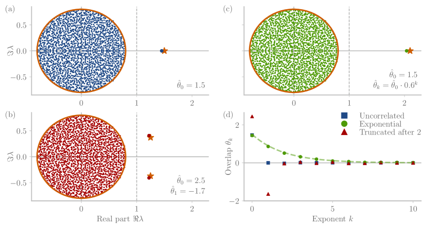
Figure 1: Spectral outliers via low-rank perturbations. Spectrum of $J+\mathbf{mn}^{T}$ with (a) no correlations, (b) exponential overlaps, and (c) truncated overlaps, Eq. 11. See Eq. 38 for details on the construction of $\mathbf{n}$. The values of non-zero $\hat{\theta}_{k}$ are displayed in each plot. Orange circles and stars indicate the theoretical prediction, dots refer to the spectra of the finite-size connectivity matrices, computed numerically. (d) Overlaps $\theta_{k}=\mathbf{n}^{T}\!J^{k}\mathbf{m}$ for the cases above. The dashed line are the target overlaps $\hat{\theta}_{k}$ for the exponential correlation. Parameters: $N=2000$, $g=0.8$.

The origin $\mathbf{x}=\mathbf{0}$ is a fixed point, since $\phi(0)=0$. It is stable if the real parts of all the eigenvalues of the Jacobian are smaller than one. Since $\phi^{\prime}(0)=1$, the Jacobian is simply the connectivity matrix $J+\mathbf{mn}^{T}$ itself. Here we examine the spectral properties of this matrix.

III.1 Eigenvalues

The spectrum of the Gaussian random matrix $J$ converges to a uniform distribution on a disk with radius $g$ and centered at the origin for $N\to\infty$ Ginibre (1965). Previous studies have explored the effect of independent low-rank perturbations like in our model Rajan and Abbott (2006); Tao (2013). They found that the limiting distribution of the remaining eigenvalues, referred to as the bulk, does not change. Additionally, the spectrum contains outliers corresponding to the eigenvalues of the low-rank perturbation itself. In this sense, the spectra of the random matrix $J$ and the low-rank perturbation decouple (although the precise location of each eigenvalue is affected by the perturbation). To our knowledge, the effect of correlated low-rank perturbations, which we explore below, has not been considered before.

To determine the spectrum, we apply the matrix determinant lemma Harville (1998):

$$\det\left(A+\mathbf{mn}^{T}\right)=\left(1+\mathbf{n}^{T}\!A^{-1}\mathbf{m}\right)\det(A)\,,$$ (3)

where $A\in\mathbb{C}^{N\times N}$ is an invertible matrix. For a complex number $z$ that is not an eigenvalue of $J$, the matrix $J-\mathds{1}z$ is invertible, resulting in

$$\begin{split}&\det\left((J+\mathbf{mn}^{T})-\mathds{1}z\right)\\ &\qquad=\left(1+\mathbf{n}^{T}\!(J-\mathds{1}z)^{-1}\mathbf{m}\right)\det(J-\mathds{1}z)\,.\end{split}$$ (4)

The roots of this equation are the eigenvalues of $J+\mathbf{mn}^{T}$. Since the determinant on the right-hand-side is nonzero, we get the scalar equation

$$z=\mathbf{n}^{T}\!\left(\mathds{1}-\frac{J}{z}\right)^{-1}\mathbf{m}\,.$$ (5)

As long as the entire spectrum is affected by the rank 1 perturbation, this equation determines all eigenvalues of $J+\mathbf{mn}^{T}$. We are interested in outliers of the spectrum: eigenvalues of $J+\mathbf{mn}^{T}$ larger than the spectral radius of $J$ (which in the limit of $N\to\infty$ is given by $g$). For such an outlier, denoted by $\lambda$, the inverse in Eq. 5 can be written as a series, and we have

$$\lambda=\sum_{k=0}^{\infty}\frac{\theta_{k}}{\lambda^{k}}\,,$$ (6)

with the overlaps

$$\theta_{k}=\mathbf{n}^{T}\!J^{k}\mathbf{m}\,.$$ (7)

Although this equation is a polynomial of infinite degree, there can be at most proper $N$ solutions (those outside of the bulk; see Appendix A).

The series representation Eq. 6 is the main result of this section. It indicates that the overlaps $\theta_{k}$ between $\mathbf{m}$ and $\mathbf{n}$ after passing through $J$ for $k$ times determine the eigenvalues of the perturbed matrix. It is hence useful to characterize the correlations between $J$ and the rank-one perturbation in terms of these overlaps.

The description up to this point is general and does not depend on details of the matrix $J$. For our model, where $J$ is a random matrix, the scalar products $\theta_{k}$ over $N$ entries are self-averaging: for $N\to\infty$, $\theta_{k}$ converges to its ensemble average $\mathbb{E}[\theta_{k}]$, with variance decaying as $1/N$. We rely on this property and compute quantities for single realization of large networks instead of ensemble averages.

A random matrix $J$ has the effect of decorrelating independent vectors: if the vectors $\mathbf{m}$ and $\mathbf{n}$ are uncorrelated to $J$, a single pass through the network already annihilates any overlap between $\mathbf{n}$ and $J\mathbf{m}$. In Appendix B, we formally show that the self-averaging indeed yields $\mathbf{n}^{T}\!J^{k}\mathbf{m}=0$ for $k\geq 1$. We can apply this to Eq. 6: If $\theta_{k}=0$ for any $k\geq 1$, then

$$\lambda=\theta_{0}=\mathbf{n}^{T}\!\mathbf{m}\,.$$ (8)

Thus an independent rank-one perturbation yields a single outlier positioned at the eigenvalue of the rank-one matrix itself [Fig. 1(a)], in accordance with known results Rajan and Abbott (2006); Tao (2013).

If $\mathbf{mn}^{T}$ is correlated to $J$, the $\theta_{k}$ will not vanish for nonzero $k$. We analyze two special cases:

1. If $\theta_{k}=0$ for any $k\geq 2$, then there are two outliers

   $$\lambda_{\pm}=\frac{\theta_{0}}{2}\pm\sqrt{\left(\frac{\theta_{0}}{2}\right)^{2}+\theta_{1}}\,.$$ (9)

   This can give rise to complex conjugate outliers, as displayed in Fig. 1(b). More generally, $K$ nonzero overlaps lead to $K$ outliers via a polynomial equation [Eq. 51].

2. A second case is one of a converging series in Eq. 6. The simplest assumption is an exponential scaling, $\theta_{k}=\theta_{0}b^{k}$ with base $b$. Inserting into the eigenvalue equation (6) yields a single solution

   $$\lambda=\theta_{0}+b\,.$$ (10)

   Remarkably, we see that correlation between the random matrix $J$ and the rank-one perturbation does not necessarily lead to more than one outlier. This is shown in Fig. 1(c). The observation generalizes to correlations expressible as a sum of $K$ exponentially decaying terms, leading to $K$ outliers [Eq. 53].

We can apply this understanding to construct a network with a set of outliers and either one of the underlying correlation structures. One way is to define the vector $\mathbf{n}$ explicitly in terms of $\mathbf{m}$ and $J$. For example, if we set

$$\mathbf{n}=\frac{1}{N}\left(\hat{\theta}_{0}\,\mathbf{m}+\frac{\hat{\theta}_{1}}{g^{2}}J\mathbf{m}\right)\,,$$ (11)

then the overlaps will self-average to $\mathbb{E}[\theta_{k}]=\hat{\theta}_{k}$ for $k\in\{0,1\}$ and $\mathbb{E}[\theta_{k}]=0$ for any $k\geq 2$, with variance scaling as $1/N$. This is shown formally and generalized to higher $\theta_{k}$ in Appendix B. The details of the construction for a set of target outliers is further detailed in Appendix C. The discrepancy between numerical and target outliers in Figure 1 is due to finite size effects, which decay with $1/\sqrt{N}$ (verified numerically, and in accordance with Ref. Mastrogiuseppe and Ostojic (2018)).

The simulations further show that the remaining eigenvalues span the same circle as without the perturbation. While all eigenvalues change, visual inspection does not reveal any changes in the statistics.

III.2 Implementation of multiple outliers

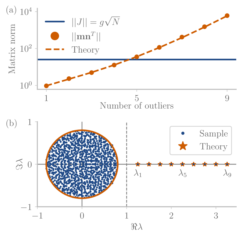
Figure 2: Scaling of the norm of the rank-one perturbation with number of induced outliers. The vector $\mathbf{n}$ is the least square solution to implementing a set of outliers $\Lambda=\{\lambda_{1},\dots,\lambda_{K}\}$, with $\lambda_{k}=1.25+0.25k$, see Appendix D. (a) Log-linear plot of the Frobenius norm of $J$ and $\mathbf{mn}^{T}$ as a function of the number of outliers. The dashed line is the theoretical prediction. (b) Spectrum of $J+\mathbf{mn}^{T}$ for $K=9$ outliers. Parameters: $N=1000$, $g=0.8$.

So far we analyzed the outliers for given correlations between $J$ and $\mathbf{mn}^{T}$ as quantified by the overlaps $\theta_{k}$. We now change the perspective and ask about the properties of the rank-one perturbation given a set of outliers. We saw that in principle a given set of outliers may have multiple underlying correlation structures – e.g. through a truncated set of non-zero overlaps or a combination of exponentially decaying terms. Regardless of the correlation structure, however, we observe that the norm of $\mathbf{n}$ grows fast with the number of outliers introduced, implying that strong perturbations are needed to generate a large number of outliers.

To understand analytically the origin of this phenomenon, we focus on a method to determine the least square $\mathbf{n}$ given $J$, $\mathbf{m}$ and the set of target outliers $\Lambda$. The resulting $\mathbf{n}$ can be formulated using the pseudoinverse, as detailed in Appendix D. The main result of this analysis is the scaling of the Frobenius norm of the rank-one matrix $\mathbf{mn}^{T}$ with the number of outliers. The asymptotic behavior is given by

$$||\mathbf{mn}^{T}||\sim g\prod_{\lambda\in\Lambda}\frac{|\lambda|}{g}\,,$$ (12)

that is, exponentially growing with the number of outliers. In comparison, the Frobenius norm of $J$ is given by $||J||=g\sqrt{N}$. This means that if one aims to place more than a handful of outliers, the perturbation $\mathbf{mn}^{T}$ becomes the dominating term (for a fixed network size $N$). We illustrate this in Fig. 2 by plotting $||\mathbf{mn}^{T}||$ for sets of outliers $\Lambda_{K}=\{\lambda_{1},\dots,\lambda_{K}\}$ with growing number $K$. The outliers $\lambda_{k}$ were placed on the real line. Further tests including complex eigenvalues gave similar results (not shown). A similar method of deriving $\mathbf{n}$ from the pseudoinverse has been described in Ref. Logiaco et al. (2019).

The scaling (12) shows another important point: the bulk radius $g$ critically determines the norm of the rank-one perturbation. Indeed, the contribution of each outlier $\lambda_{k}$ is relative to the radius. Even for a single outlier, where

$$||\mathbf{mn}^{T}||=\sqrt{\lambda^{2}-g^{2}}\,,$$ (13)

an increase in $g$ leads to decreasing norm. This observation suggests that a large random connectivity facilitates the control of the spectrum by a rank-one perturbation.

IV Non-trivial fixed points

We now turn to the non-trivial fixed points of the network. At these, the internal states $\mathbf{x}$ obey the equation

$$\mathbf{x}=J\bm{\phi}+\kappa\mathbf{m}\,.$$ (14)

Here we defined the scalar feedback strength $\kappa=\mathbf{n}^{T}\!\bm{\phi}$, using the vector notation $\bm{\phi}=\phi(\mathbf{x})$.

The fixed points of related models have been analyzed in previous works. For infinitely large networks, the unperturbed system ($P=0$) has a single fixed point at the origin if $g<1$ Wainrib and Touboul (2013). For $g>1$, the system exhibits chaotic dynamics Sompolinsky et al. (1988). In this regime, the number of (unstable) fixed points scales exponentially with the network size $N$ Wainrib and Touboul (2013). Here we only focus on networks in the non-chaotic regime, where either $g<1$ or the perturbation $P$ suppresses chaos Mastrogiuseppe and Ostojic (2018).

IV.1 Fixed point manifold

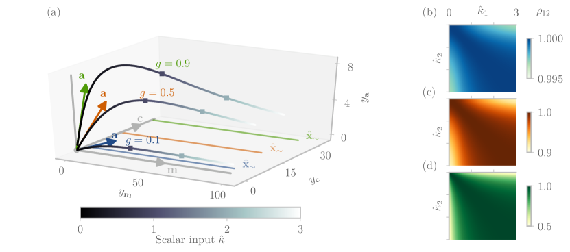
Figure 3: Manifold $\mathcal{M}$, Eq. 16 constraining fixed points, Eq. 15. (a) Projection of $\mathcal{M}$ for three networks with different strength of randomness $g$ (see main text for the three-dimensional basis). The negative side for $\hat{\kappa}<0$ is symmetric and not shown. The squares on the manifolds indicate the inputs $\hat{\kappa}=(1,2)$. The straight lines in the plane $y_{\mathbf{a}}=0$ are the asymptotic directions $\hat{\mathbf{x}}_{\sim}$ for the manifolds. (b-d) Correlation $\rho_{12}$ between two points $\hat{\mathbf{x}}(\hat{\kappa}_{i})$ on $\mathcal{M}$ for two different inputs $\hat{\kappa}_{1},\hat{\kappa}_{2}\in[0,3]$. (b, c, d) correspond to the random connectivity strengths $g=0.1,0.5,0.9$, respectively. Note the different scales on the color bars.

Following Rivkind and Barak (2017), the perturbed system with fixed points (14) can be understood using a surrogate system in which the feedback $\kappa$ is replaced with a fixed scalar $\hat{\kappa}$. For $g<1$, every such value $\hat{\kappa}$ corresponds to a unique fixed point

$$\hat{\mathbf{x}}=J\phi(\hat{\mathbf{x}})+\hat{\kappa}\mathbf{m}\,.$$ (15)

This equation defines the one-dimensional nonlinear manifold

$$\mathcal{M}=\{\hat{\mathbf{x}}\,|\,\hat{\kappa}\in\mathbb{R}\}\,.$$ (16)

The manifold $\mathcal{M}$ can be understood by looking at the asymptotics. For large input $\hat{\kappa}$, the nonlinearity saturates and the manifold becomes approximately linear:

$$\hat{\mathbf{x}}_{\sim}=\mathbf{c}+\hat{\kappa}\mathbf{m}\,,$$ (17)

with $\mathbf{c}=J\,\mathrm{sign}(\mathbf{m})$. Around the origin, we linearize and obtain

$$\hat{\mathbf{x}}=\hat{\kappa}\,\mathbf{a}+\mathcal{O}(\hat{\kappa}^{2})\,,$$ (18)

with $\mathbf{a}=\left(\mathds{1}-J\right)^{-1}\mathbf{m}$.

Applying orthonormalization to the triplet $(\mathbf{m,c,a})$, we obtain a three-dimensional basis. We observe that, for $N\to\infty$, the vectors $\mathbf{m}$ and $\mathbf{c}$ are orthogonal and that the vector $\mathbf{a}$ becomes orthogonal to the other two in the limit $g\to 1$. Accordingly, we name the coefficients of the basis $(y_{\mathbf{m}},y_{\mathbf{c}},y_{\mathbf{a}})$. The projection of the manifold $\mathcal{M}$ on this basis is shown in Fig. 3(c) for three different values of $g$. Numerical evaluation of the reconstruction error shows that these three dimensions reconstruct the manifold very well albeit with decreasing accuracy for increasing $g$ (not shown).

Fixed points of the full system are obtained by determining $\kappa$ self-consistently. They necessarily lie on the manifold $\mathcal{M}$. One consequence is a strong correlation between pairs of fixed points, especially if both lie close to the origin or in the saturating regime. In Fig. 3(b-d), we numerically evaluate this correlation for three different randomness strengths $g$. On can observe that for $g\leq 0.5$, correlation does not drop below 90%. Even for $g=0.9$, the correlation is low only if one fixed point is very close to the origin and the other one is far out.

So far we only considered the case $g<1$. For $g>1$, there is a minimal $\hat{\kappa}_{\mathrm{min}}$ for which the dynamics are stabilized and a unique stable fixed point emerges Mastrogiuseppe and Ostojic (2018). Here, the manifold $\mathcal{M}$ is unconnected and now reads $\mathcal{M}=\{\hat{\mathbf{x}}\,|\,\hat{\kappa}\in\mathbb{R}\setminus(-\hat{\kappa}_{\mathrm{min}},\hat{\kappa}_{\mathrm{min}})\}$.

Finally we note that the constraints of a one-dimensional manifold are general and do not depend on the details of the vector $\mathbf{n}$, especially not on its Gaussian statistics. This is particularly important for learning algorithms like the echo state framework or FORCE, which by construction only allow for the adaptation of the vector $\mathbf{n}$ Jaeger and Haas (2004); Sussillo and Abbott (2009). Accordingly, fixed points in these cases are also strongly correlated, which may lead to catastrophic forgetting when trying to learn multiple fixed points sequentially Beer and Barak (2019).

IV.2 Mean field theory

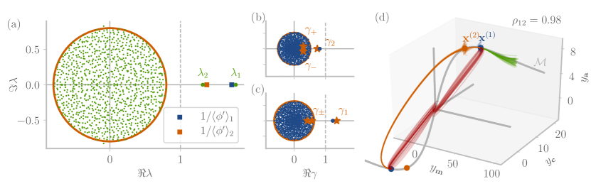
Figure 4: Two fixed points induced by rank-one perturbation correlated to the random connectivity $J$. (a) Spectrum of $J+\mathbf{mn}^{T}$. The squares indicate the corresponding averaged slopes at the fixed points, as predicted by Eq. 26. (b-c) Eigenvalues of the Jacobian at the two fixed points $\mathbf{x}^{(1)}$ (b) and $\mathbf{x}^{(2)}$ (c). Stars indicate the theoretical predictions for exceptional stability eigenvalues (only meaningful outside the bulk). (d) Fixed points and manifold $\mathcal{M}$. The colored lines indicate trajectories starting from the two fixed points (blue and orange), a point on the manifold $\mathcal{M}$ (green) and the origin. All trajectories converge on $\mathbf{x}^{(1)}$ or its negative counterpart. At each point, 50 different initial conditions are obtained by adding Gaussian noise (SD = 0.5). The fixed point correlation is indicated by $\rho_{12}$. Parameters: $g=0.8$, $N=1000$. The rank-one perturbation is obtained by the least-squared $\mathbf{n}$, see Appendix D.

For non-trivial fixed points of the full network, Eq. 14, the scalar feedback $\kappa$ needs to be consistent with the firing rates $\phi(\mathbf{x})$. Similar to prior works, we compute $\kappa$ using a mean field theory Mastrogiuseppe and Ostojic (2018). The central idea of the mean field theory is to replace the input to each variable $x_{i}$ by a stochastic variable with statistics matching the original system. The statistics of the resulting stochastic processes $x_{i}$ are then computed self-consistently.

Because our model includes correlations between the random part $J$ and the low-rank structure $P$, the correlations in the activity do not vanish as dynamics unfold. This phenomenon prevents the application of previous theories Mastrogiuseppe and Ostojic (2018). We hence develop a new theory. The details are elaborated in Appendix E. Here we give an outline of the analysis.

The starting point is the scalar feedback $\kappa$. The Gaussian statistics of $\mathbf{n}$ and the fixed point $\mathbf{x}$ allow to factor out the effect of the nonlinearity via partial integration. We have

$$\kappa=\mathbf{n}^{T}\!\bm{\phi}=\langle\phi^{\prime}\rangle\,\mathbf{n}^{T}\!\mathbf{x}\,,$$ (19)

with the average slope $\langle\phi^{\prime}\rangle$ evaluated at the fixed point:

$$\langle\phi^{\prime}\rangle=\int\mathcal{D}z\,\phi^{\prime}(\sqrt{\Delta^{0}}z)\,,$$ (20)

where $\mathcal{D}z$ is the standard Gaussian measure. $\Delta^{0}$ is the variance of $\mathbf{x}$, which from the fixed point equation (14) is given by

$$\Delta^{0}=g^{2}\langle\phi^{2}\rangle+\kappa^{2}\,.$$ (21)

The quantities $\langle\phi^{\prime}\rangle$, $\Delta^{0}$, and $\kappa$ are determined self-consistently. To that end, we further evaluate $\kappa$ in Eq. 19. Inserting the fixed point equation (14) yields

$$\mathbf{n}^{T}\!\mathbf{x}=\mathbf{n}^{T}\!J\bm{\phi}+\kappa\mathbf{n}^{T}\!\mathbf{m}\,.$$ (22)

The first term on the right-hand side vanished in previous studies with no correlation between $P$ and $J$ Mastrogiuseppe and Ostojic (2018). In our case, there are correlations, and we proceed to analyze this term. We first interpret $J^{T}\mathbf{n}$ as a Gaussian vector and use partial integration to replace $\bm{\phi}$ with $\mathbf{x}$:

$$\mathbf{n}^{T}\!\mathbf{x}=\langle\phi^{\prime}\rangle\mathbf{n}^{T}\!J\mathbf{x}+\kappa\mathbf{n}^{T}\!\mathbf{m}\,.$$ (23)

We now insert the fixed point equation (14) into the new first term of the right hand side. We can apply this scheme recursively and arrive at an equation linear in $\kappa$ on both sides:

$$\kappa=\kappa\langle\phi^{\prime}\rangle\,\sum_{k=0}^{\infty}\langle\phi^{\prime}\rangle^{k}\,\theta_{k}\,,$$ (24)

with overlaps as defined above, Eq. 7. We are looking at a non-trivial fixed point, so we can divide by the nonzero $\kappa$ to obtain

$$\frac{1}{\langle\phi^{\prime}\rangle}=\sum_{k=0}^{\infty}\langle\phi^{\prime}\rangle^{k}\,\theta_{k}\,.$$ (25)

A comparison with Eq. 6 shows that the two equations are identical if

$$\lambda=1/\langle\phi^{\prime}\rangle\,.$$ (26)

This is a remarkable relationship between the outliers and autonomously generated fixed points: each non-trivial fixed point $\mathbf{x}^{(i)}$ must be associated with a real eigenvalue $\lambda_{i}$ such that the average over the derivative of firing rates at this fixed point, $\langle\phi^{\prime}\rangle_{i}$, fulfills the above condition (26). In the special case of $\phi=\mathrm{tanh}$, the $\langle\phi^{\prime}\rangle_{i}$ are confined to the interval $(0,1]$, so the corresponding eigenvalues must be real and larger than one. One may hence look at the spectrum of the connectivity matrix alone and determine how many non-trivial fixed points there are. An instance of this phenomenon is illustrated in Fig. 4. The spectrum at the origin contains two outliers $\lambda_{i}$, $i=1,2$, each real and larger than one. The dynamics have two corresponding fixed points $\mathbf{x}^{(i)}$ located on the manifold $\mathcal{M}$. In accordance with Eq. 26, the average slopes at these fixed points, $1/\langle\phi^{\prime}\rangle_{i}$, agree with the outliers up to deviations due to the finite network size.

IV.3 Stability of fixed points

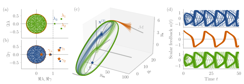
Figure 5: Limit cycle induced by oscillatory instability. (a) Spectrum of the connectivity matrix. The outlier $\lambda_{3}$ is real-valued and larger than one, so there is a corresponding fixed point $\mathbf{x}_{3}$. (b) The spectrum at the fixed point. The predicted stability eigenvalue $\gamma_{-}$ lies inside the bulk and is not labeled. (c) Fixed point and dynamics as in Fig. 4. Trajectories start at the fixed point (blue), a point on the manifold $\mathcal{M}$ (orange) and the origin (green). (d) Scalar feedback $\kappa(t)$ for the different initial conditions. Parameters: $g=0.6$, $N=1000$. The rank-one perturbation is obtained by the least-squared $\mathbf{n}$, see Appendix D.

The stability of each fixed point is determined by the spectrum of its Jacobian. The associated stability matrix (the Jacobian shifted by $-\mathds{1}$) is

$$S=\left(J+\mathbf{m}\mathbf{n}\right)R^{\prime}\,,$$ (27)

with the diagonal matrix of slopes $R_{ij}^{\prime}=\delta_{ij}\phi_{i}^{\prime}$. Previous work (Mastrogiuseppe and Ostojic (2018)) has found that the spectrum of $S$, too, consists of a bulk and a small number of exceptional eigenvalues: in the case of an uncorrelated rank-one perturbation, there are two nonzero eigenvalues obtained via mean field theory, only one of which has been found outside the random bulk. The radius of the bulk shrinks to $g\sqrt{\langle\phi^{\prime 2}\rangle}$ due to the saturation of the nonlinearity Mastrogiuseppe and Ostojic (2018). We find numerically that the bulk behaves alike in our model, too. For the rest of this section, however, we focus on exceptional eigenvalues of the stability matrix $S$, denoted by $\gamma$.

Similar to the trivial fixed point, one can apply the matrix determinant lemma to derive an equation for the stability eigenvalues:

$$\gamma=\mathbf{n}^{T}\!R^{\prime}\left(\mathds{1}-\frac{JR^{\prime}}{\gamma}\right)^{-1}\mathbf{m}\,.$$ (28)

We can apply the mean field theory introduced above to evaluate the right hand side. The details of this calculation are deferred to Appendix F. It turns out that the resulting $\gamma$ are surprisingly compact. We now describe these stability eigenvalues.

Consider the fixed point $\mathbf{x}^{(i)}$. According to Eq. 26, this fixed point corresponds to the eigenvalue $\lambda_{i}$. Eq. 28 always has two solutions $\gamma_{\pm}$ determined by a quadratic equation. These are only dependent on the outlier $\lambda_{i}$ and the statistics of the fixed point $\mathbf{x}^{(i)}$, but entirely independent of the remaining spectrum or other fixed points. Their precise values are detailed in Eq. 100. It turns out that $\gamma_{+}$ and $\gamma_{-}$ always have a real part smaller than one. They hence do not destabilize the fixed point. Additionally, at least one of the two is always hidden within the bulk of the eigenvalues, as observed before for the case of no correlation Mastrogiuseppe and Ostojic (2018). In Fig. 4(b-c), the spectra of the Jacobian at two fixed points are compared with the theoretical predictions. In both cases, $\gamma_{\pm}$ correspond to the two stars within the bulk. In Fig. 5(b), the bulk is smaller ($g=0.6$) and $\gamma_{+}$ is visible.

If $\lambda_{i}=\lambda_{1}$ is the only outlier, then $\gamma_{\pm}$ are the only two solutions of Eq. 28, and the fixed point $\mathbf{x}^{(1)}$ as well as its mirror $-\mathbf{x}^{(1)}$ will be stable. However, if there are $K\geq 2$ outliers $\{\lambda_{1},\dots,\lambda_{K}\}$, we find an additional set of $K-1$ stability eigenvalues

$$\gamma_{j}=\frac{\lambda_{j}}{\lambda_{i}}\quad\text{for all}\quad j\in\{1,\dots,K\},\,j\neq i\,.$$ (29)

This expression indicates a remarkable relationship between different fixed points: the existence of a fixed point $\mathbf{x}^{(j)}$ with outlier $\lambda_{j}>\lambda_{i}$ will always destabilize the fixed point $\mathbf{x}^{(i)}$ corresponding to $\lambda_{i}$. Conversely, if there are no outliers with real part larger than that of $\lambda_{i}$, then $\mathbf{x}^{(i)}$ will be stable. Since $\lambda=1/\langle\phi^{\prime}\rangle$ implies that larger $\lambda$ corresponds to larger fixed point variance $\Delta^{0}$, one can say that only the largest fixed point can be stable, Such an interaction between two fixed points is illustrated in Fig. 4(b-c). The stars outside of the bulk correspond to the predicted eigenvalue $\gamma_{2}$ or $\gamma_{1}$. Comparison between the theoretical prediction (29) and numerical calculation for a sampled network shows good agreement for both fixed points. Furthermore, a simulation of the dynamics in Fig. 4(d) shows that indeed all trajectories converge to the larger fixed point $\mathbf{x}^{(1)}$ or its negative counterpart.

Finally, note that a complex outlier $\lambda_{j}$ also destabilizes a fixed point $\mathbf{x}^{(i)}$ if the real part of $\lambda_{j}$ is larger than that of $\lambda_{i}$. Complex outliers do not have corresponding fixed points, since Eq. 26 is real. An example of such a case is shown in Fig. 5. There is only one real eigenvalue larger than one, and hence only a single non-trivial fixed point $\mathbf{x}^{(3)}$. Nonetheless, the two complex outliers $\lambda_{1}=\lambda_{2}^{*}$ destabilize the fixed point by virtue of Eq. 29, since the real parts are larger than the outlier corresponding to the fixed point, $\Re\lambda_{1}=\Re\lambda_{2}>\lambda_{3}$. Numerical simulations indicate that in such a case, the dynamics converge on a limit cycle.

V rank-two perturbations

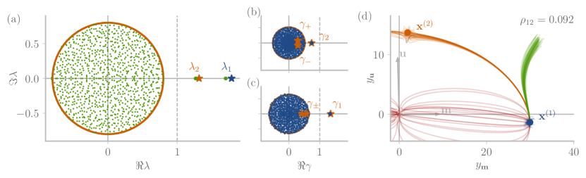
Figure 6: Fixed points and dynamics for a rank-two perturbation with structures $\mathbf{mn}^{T}$ and $\mathbf{uv}^{T}$ drawn independently of each other as well as of $J$. (a-c) Spectra of the Jacobian at the origin (a) and at the two fixed points $\mathbf{x}^{(1)}$ (b) and $\mathbf{x}^{(2)}$ (c). Stars denote the predictions for infinite size networks. (d) Projection of fixed points on vectors $\mathbf{m}$ and $\mathbf{u}$, and trajectories starting around $\mathbf{x}^{(1)}$ (blue), $\mathbf{x}^{(2)}$ (orange), $\mathbf{x}^{(1)}+\mathbf{x}^{(2)}$ (green) and $\mathbf{0}$ (red). The correlation between the two fixed points is indicated by $\rho_{12}$. Other parameters as in Fig. 4.

The previous section demonstrated two properties of networks with multiple non-trivial fixed points: they are highly correlated due to the confinement on the manifold $\mathcal{M}$ [Fig. 3(b-d) and Fig. 4(d)], and their stability properties interact [Eq. 29]. We asked whether the latter is a result of the former. To approach this question, we extend the model to a rank-two perturbation which allows for uncorrelated fixed points.

The rank-two connectivity structure is defined by

$$P=\mathbf{m}\mathbf{n}^{T}+\mathbf{u}\mathbf{v}^{T}\,.$$ (30)

We assume $J$, $\mathbf{m}$ and $\mathbf{u}$ to be drawn independently. Similar to the rank-one case, the entries of both $\mathbf{m}$ and $\mathbf{u}$ are drawn from standard normal distributions while $\mathbf{n}$ and $\mathbf{v}$ are Gaussian and dependent on $J,\mathbf{m}$ and $\mathbf{u}$.

The outliers $\lambda$ of the perturbed matrix $J+\mathbf{mn}^{T}\!+\mathbf{uv}^{T}$ are calculated similarly to the rank-one case. Applying the matrix determinant lemma twice, we arrive at an equation of quadratic form:

$$0=\lambda^{2}-\lambda\mathrm{Tr}Q_{\lambda}+\det(Q_{\lambda})\,.$$ (31)

In other words, $\lambda$ is an eigenvalue of the matrix

$$Q_{\lambda}=\begin{bmatrix}\mathbf{n}^{T}\!M_{\lambda}\mathbf{m}&\mathbf{n}^{T}\!M_{\lambda}\mathbf{u}\\ \mathbf{v}^{T}\!M_{\lambda}\mathbf{m}&\mathbf{v}^{T}\!M_{\lambda}\mathbf{u}\end{bmatrix}\,,$$ (32)

which depends on $\lambda$ through

$$M_{\lambda}=\left(\mathds{1}-\frac{J}{\lambda}\right)^{-1}\,.$$ (33)

In general there are more than two solutions, but if the rank-two perturbation is uncorrelated to $J$, the matrix $M_{\lambda}$ disappears in $Q_{\lambda}$. The solution is then in agreement with previous results Mastrogiuseppe and Ostojic (2018).

Non-trivial fixed points of the network dynamics (2) with a rank-two perturbation (30) obey the equation

$$\mathbf{x}=J\bm{\phi}+\kappa_{1}\mathbf{m}+\kappa_{2}\mathbf{u}\,,$$ (34)

with $\kappa_{1}=\mathbf{n}^{T}\!\bm{\phi}$ and $\kappa_{2}=\mathbf{v}^{T}\!\bm{\phi}$. Similar to the rank-one case, we can apply the recursive insertion of the fixed point and partial integration, Eqs. 19 and 22, to compute the two-component vector $\bm{\kappa}=(\kappa_{1},\kappa_{2})$. We arrive at

$$Q_{\lambda}\bm{\kappa}=\frac{1}{\langle\phi^{\prime}\rangle}\bm{\kappa}\,.$$ (35)

This equation has two consequences: First, we find that $\lambda=1/\langle\phi^{\prime}\rangle$, because both sides are eigenvalues of $Q_{\lambda}$, see Eq. 31. Second, the feedback vector $\bm{\kappa}$ is the corresponding eigenvector. This gives rise to three situations:

1. If $Q_{\lambda}$ has two distinct eigenvalues, one of them is equal to $\lambda$. The corresponding eigenvector determines the direction of $\bm{\kappa}$.

In the case of degeneracy, the geometric multiplicity, that is, the number of eigenvectors, determines the situation.

1. If there is only one eigenvector, the direction of $\bm{\kappa}$ is determined uniquely.

2. If $\lambda$ has two corresponding eigenvectors, any direction is a solution. The length of $\bm{\kappa}$ is determined below, Eq. 36, and we obtain a ring attractor Mastrogiuseppe and Ostojic (2018). This situation arises in the case of precise symmetry, $Q_{\lambda}=\lambda\mathds{1}$.

Finally, the length of $\bm{\kappa}$ is determined by the variance $\Delta^{0}=\mathbf{x}^{T}\!\mathbf{x}/N$ of the fixed point, which obeys

$$\Delta^{0}=g^{2}\langle\phi^{2}\rangle+\kappa_{1}^{2}+\kappa_{2}^{2}\,.$$ (36)

The fixed point stability is calculated based on the techniques introduced above; details can be found in Appendix H. The result is the same as that in the rank-one case: the stability eigenvalues obey the same equations as before. Namely, if the spectrum of $J+\mathbf{mn}^{T}+\mathbf{uv}^{T}$ has the outliers $\{\lambda_{1},\dots,\lambda_{K}\}$, there are always two stability eigenvalues $\gamma_{\pm}$, both with real parts smaller than one. At a fixed point $\mathbf{x}^{(i)}$, there are $K-1$ additional outliers $\gamma_{j}=\lambda_{j}/\lambda_{i}$ for $j\neq i$. This implies that linear dynamics around a fixed point is completely determined by its statistics and the spectrum of the connectivity matrix: as long as the outliers are the same, the stability eigenvalues are independent of the rank of the perturbation $P$ or its correlations to $J$.

This also answers our question about whether the correlation between fixed points is responsible for the strong influence on each other. The rank-two case, too, can be analyzed by replacing the feedback $\kappa_{1},\kappa_{2}$ with two constant scalars. The corresponding manifold is now two-dimensional, and fixed points can be arbitrarily uncorrelated. In Fig. 6, we show an example: plotting the projection of the fixed points along the vectors $\mathbf{m}$ and $\mathbf{u}$ shows that the fixed points are almost orthogonal. Yet, the spectra at the origin and at each fixed point are identical to the corresponding rank-one case (compare with Fig. 4). The correlation between fixed points is hence not important for the mutual influence of different fixed points.

VI Discussion

Given a network with connectivity consisting of a random and a structured part, we examined the effects of correlations between the two. We found that such correlations enrich the functional repertoire of the network. This is reflected in the number of non-trivial fixed points and the spectrum of the connectivity matrix. We analyzed precisely which aspects of the correlations determine the fixed points and eigenvalues.

In our model, the overlaps $\theta_{k}=\mathbf{n}^{T}J^{k}\mathbf{n}$ quantify the correlations between random connectivity $J$ and structured, low-rank connectivity $\mathbf{mn}^{T}$. For uncorrelated networks, only $\theta_{0}$ is nonzero, and the spectrum of the joint connectivity matrix has only a single outlier Rajan and Abbott (2006); Tao (2013). We showed that in correlated networks with $\theta_{k}$ nonzero for higher $k$, multiple outliers can exist, and that with such, multiple fixed points induced by a random plus rank-one connectivity structure become possible. The correlations between random part and rank-one structure hence enrich the dynamical repertoire in contrast to networks with uncorrelated rank-one structures, which can only induce a single fixed point Mastrogiuseppe and Ostojic (2018). Note, however, that our assumption of Gaussian connectivity limits the resulting dynamics to a single stable fixed point (discussed below).

Apart from multiple fixed points, the correlated rank-one structure can also lead to a pair of complex conjugate outliers, which in turn yield oscillatory dynamics on a limit cycle. In absence of correlations, such dynamics need the perturbation to be at least of rank two Mastrogiuseppe and Ostojic (2018). Finally, we found that correlations amplify the perturbation due to the structured components: the norm of a correlated rank-one structure inducing a fixed point decreases with increasing variance of the random part, pointing towards possible benefits of large initial random connectivity.

Constraining the model to Gaussian connectivity allowed us to analytically understand the mechanisms of correlations in a nonlinear network. We established a remarkable one-to-one correspondence between the outliers of the connectivity matrix and fixed points of the nonlinear dynamics: each real outlier larger than one induces a single fixed point. Surprisingly, the stability of the fixed points is governed by a simple set of equations and also only depend on the outliers of the spectrum at the origin. Through these results, we were able to look at the system at one point in phase space (the origin) and determine its dynamics at a different part of the phase space. It remains an open question to which degree these insights extend to non-Gaussian connectivity. Interesting other connectivity models might include sparse connectivity Neri and Metz (2012, 2016); Metz et al. (2019), different neuron types Aljadeff et al. (2015), or networks of binary neurons such as the Hopfield model Hopfield (1982).

Our approach allows us to gain mechanistic insight into the computations underlying echo state and FORCE learning models which have the same connectivity structure as our model Jaeger and Haas (2004); Sussillo and Abbott (2009). Here, the readout vector $\mathbf{n}$ is trained, which leads to correlations to the random part $J$ Rivkind and Barak (2017); Mastrogiuseppe and Ostojic (2019). Our results on multiple fixed points and oscillations show that these correlations are crucial for the rich functional repertoire. However, constraining our theory to Gaussian connectivity limits the insights, since the learning frameworks do not have this constraint. One study analyzing such non-Gaussian rank-one connectivity in the echo state framework shows that, like in our study, each fixed point had one corresponding outlier in the connectivity matrix Rivkind and Barak (2017). However, multiple stable fixed points were observed, which is in contrast to our model where the Gaussian connectivity only permits the fixed point with largest variance to be stable. It would thus be interesting to extend our model beyond the Gaussian statistics.

We pointed out a general limitation of networks with random plus rank-one connectivity: the restriction of fixed points to a one-dimensional manifold. This insight is independent of the Gaussian assumption and leads to high correlations between fixed points. Such correlations have been found to impede sequential learning of multiple fixed points Beer and Barak (2019). An extension to rank-two structures allows for uncorrelated fixed points. Surprisingly, however, the strong influence of the largest outliers on the stability of fixed points still exists for Gaussian rank-two connectivity. Indeed, the fixed point statistics and their stability is determined solely by the spectral outliers of the connectivity matrix, independently of how these outliers were generated. Since these relations do not hold in the non-Gaussian case, Rivkind and Barak (2017), we conclude that the Gaussian assumption poses a severe limitation to the space of solutions.

Further in accordance with the echo state and FORCE learning frameworks Jaeger and Haas (2004); Sussillo and Abbott (2009), we model the correlations to be induced by one of the two vectors forming the rank-one structure. Some of the results, such as the overlaps $\theta_{k}$, are symmetric under the exchange of the two vectors and should hence be unaffected. The result on the strongly increasing norm of the perturbation when placing multiple outliers, on the other hand, may depend on this assumption Logiaco et al. (2019). To which degree our results or the capabilities of trained networks are limited by this constraint is not clear.

Our choice to model the structured part as a low-rank matrix was in part motivated by the computational models discussed above. Besides these, the existence of such structures may also be inspired by a biological perspective. Any feedback loop from a high-dimensional network through an effector with a small number of degrees of freedom may be considered as a low-rank perturbation to the high-dimensional network. Similarly, feedback loops from cortex through basal ganglia have been modeled as low-rank connectivity Logiaco et al. (2019). Even without such explicit loops, networks may effectively have such structure if their connectivity is scale-free or contains hubs Rivkind et al. (2019). Finally, low-rank connectivity also appears outside of neuroscience, for example in an evolutionary setting Furusawa and Kaneko (2018). Whether low-rank matrices arise in general in learning networks, and to which degree such structure is correlated with the initially present connectivity are interesting future questions to be approached with the theory we developed here.

Appendix A Finite number of solutions for outliers

Eq. 6 in the main text is a polynomial of infinite degree. It may thus seem that there are infinite solutions for the outlying eigenvalues, even in the case of a finite network of size $N$. We now show why this is not the case. Note that the equation was only valid for outliers (enabling the series expansion). Denote the eigenvalues of $J$ by $\hat{\lambda}_{i}$, $1\leq i\leq N$. If we diagonalize $J=L^{T}\hat{\Lambda}R$ with $\hat{\Lambda}=\mathrm{diag}(\hat{\lambda_{1}},\dots,\hat{\lambda}_{N})$, and write $\hat{\mathbf{n}}=L\mathbf{n}$ and $\hat{\mathbf{m}}=R\mathbf{m}$, then the series becomes

$$\lambda=\sum_{k=0}^{\infty}\frac{\sum_{i=1}^{N}\hat{n}_{i}\hat{\lambda}_{i}^{k}\hat{m}_{i}}{\lambda^{k}}=\sum_{i=1}^{N}\frac{\hat{n}_{i}\hat{m}_{i}}{1-\frac{\hat{\lambda}_{i}}{\lambda}}\,,$$ (37)

which is a polynomial equation of degree $N$.

Appendix B Construction of the vector n

In our model, $J$ and $\mathbf{m}$ are drawn independently from Gaussian distributions. We construct $\mathbf{n}$ from the these two quantities for a target set of overlaps $\hat{\theta}_{k}$. Specifically, we set

$$\mathbf{n}=\frac{1}{N}\sum_{k=0}^{\infty}\frac{\hat{\theta}_{k}}{g^{2k}}J^{k}\mathbf{m}\,.$$ (38)

Below we show that with this definition the actual overlaps $\theta_{k}$ converge to the targets $\hat{\theta}_{k}$ with increasing network size $N$. Note that the scaling by $1/N$ renders the $\theta_{k}$ order one quantities.

We start by analyzing the uncorrelated case, for which $\hat{\theta}_{k}=0$ for any $k\geq 1$, and

$$\mathbf{n}=\frac{\hat{\theta}_{0}}{N}\mathbf{m}\,.$$ (39)

We need to show that $\theta_{0}$ converges to $\hat{\theta}_{0}$ as $N\to\infty$. To this end, we will show that the expected value has this limit and that the variance vanishes. We calculate the scalar product

$$\theta_{0}=\mathbf{n}^{T}\!\mathbf{m}=\hat{\theta}_{0}\,\frac{\mathbf{m}^{T}\!\mathbf{m}}{N}\,.$$ (40)

The expected value of $\mathbf{m}^{T}\!\mathbf{m}/N$ is one, so we observe that, indeed, $\mathbb{E}[\theta_{0}]=\hat{\theta}_{0}$. For the variance we have

$$\begin{split}\mathrm{var}\left(\frac{\mathbf{m}^{T}\!\mathbf{m}}{N}\right)&=\frac{1}{N^{2}}\sum_{ij}\mathbb{E}[m_{i}^{2}m_{j}^{2}]-1\\ &=\frac{1}{N^{2}}\sum_{ij}\mathbb{E}[m_{i}^{2}]\mathbb{E}[m_{j}^{2}]-1\\ &\quad+\frac{1}{N^{2}}\left(\sum_{i}\mathbb{E}[m_{i}^{4}]-\sum_{i}\mathbb{E}[m_{i}^{2}]^{2}\right)\\ &=\mathcal{O}\left(\frac{1}{N}\right)\,.\end{split}$$ (41)

The term in the second line vanishes, and the one in line three is of order $\mathcal{O}(1/N)$ since the fourth moment does not depend on the network size. The scalar product hence has a self-averaging quality in the sense that it converges to its expected value with deviations on the order $\mathcal{O}(1/\sqrt{N})$.

The next overlap is treated similarly:

$$\theta_{1}=\mathbf{n}^{T}\!J\mathbf{m}=\frac{\hat{\theta}_{0}}{N}\sum_{ij}m_{i}J_{ij}m_{j}\,.$$ (42)

Here, the expected value is equal to zero because of the independence between $J$ and $\mathbf{m}$. The variance decays with $N$ as before:

$$\begin{split}\mathrm{var}\left(\theta_{1}\right)&=\left(\frac{\hat{\theta}_{0}}{N}\right)^{2}\sum_{ijkl}\mathbb{E}[m_{i}J_{ij}m_{j}\,m_{k}J_{kl}m_{l}]\\ &=\left(\frac{\hat{\theta}_{0}}{N}\right)^{2}\sum_{ij}\mathbb{E}[m_{i}^{2}J_{ij}^{2}m_{j}^{2}]\\ &=\left(\frac{\hat{\theta}_{0}}{N}\right)^{2}\sum_{ij}\mathbb{E}[m_{i}^{2}m_{j}^{2}]\,\frac{g^{2}}{N}\\ &=\theta_{0}^{2}g^{2}\left(\frac{1}{N}+\frac{2}{N^{2}}\right)\\ &=\frac{\theta_{0}^{2}g^{2}}{N}+\mathcal{O}\left(\frac{g^{2}}{N^{2}}\right)\,.\end{split}$$ (43)

The off-diagonal terms in the first line disappear since entries with different indices are independent. Similar calculations can be done for any of the higher order overlaps $\theta_{k}$, and one finds that the variance of these terms is

$$\mathrm{var}(\theta_{k})=\frac{\theta_{0}^{2}g^{2k}}{N}+\mathcal{O}\left(\frac{g^{2k}}{N^{2}}\right)\,.$$ (44)

We now turn to the correlated case. Here, the terms $\hat{\theta}_{k}$ may be non-zero. We only discuss the simplest case with $\hat{\theta}_{k}=0$ for any $k\geq 2$, since all other cases can be treated similarly. We write

$$\mathbf{n}=\frac{1}{N}\left(\hat{\theta}_{0}\mathbf{m}+\frac{\hat{\theta}_{1}}{g^{2}}J\mathbf{m}\right)\,,$$ (45)

and calculate the zeroth overlap

$$\theta_{0}=\hat{\theta}_{0}\,\frac{\mathbf{m}^{T}\!\mathbf{m}}{N}+\frac{\hat{\theta}_{1}}{g^{2}}\,\cancel{\frac{\mathbf{m}^{T}\!J\mathbf{m}}{N}}\,.$$ (46)

The crossed-out term self-averages to zero due to the independence between $J$ and $\mathbf{m}$, so that $\mathbb{E}[\theta_{0}]=\hat{\theta_{0}}$.

Similar reasoning applies to the first overlap:

$$\theta_{1}=\hat{\theta}_{1}\,\cancel{\frac{\mathbf{m}^{T}\!J^{T}\mathbf{m}}{N}}+\frac{\hat{\theta}_{1}}{g^{2}}\,\frac{\mathbf{m}^{T}\!J^{T}J\mathbf{m}}{N}\,.$$ (47)

Now, however, it is the first term that vanishes. The second one remains order $\mathcal{O}(1)$:

$$\begin{split}\mathbb{E}\left[\frac{\mathbf{m}^{T}\!J^{T}J\mathbf{m}}{N}\right]&=\frac{1}{N}\sum_{ijk}\mathbb{E}[m_{i}J_{ji}J_{jk}m_{k}]\\ &=\frac{1}{N}\sum_{ij}\mathbb{E}[m_{i}^{2}]\mathbb{E}[J_{ji}^{2}]\\ &=g^{2}\,,\end{split}$$ (48)

and hence $\mathbb{E}[\theta_{1}]=\hat{\theta}_{1}$. Similar calculations show that

$$\mathrm{var}\left(\frac{\mathbf{m}^{T}\!J^{T}J\mathbf{m}}{N}\right)=\frac{2g^{4}}{N}+\mathcal{O}\left(\frac{g^{4}}{N^{2}}\right)\,,$$ (49)

where the factor 2 is of combinatorial nature, counting how many index combinations yield nonzero expectations.

The last calculations explain the scaling by $1/g^{2k}$ in the definition of $\mathbf{n}$, Eq. 38. It also points to a general feature of the algebra of scalar products: products of the sort $\mathbf{a}(J^{T})^{k}J^{l}\mathbf{b}$ for vectors $\mathbf{a}$ and $\mathbf{b}$ independent of $J$ yield the expected value

$$\mathbb{E}\left[\mathbf{a}^{T}\!(J^{T})^{k}J^{l}\mathbf{b}\right]=\begin{cases}g^{2k}\mathbf{a}^{T}\!\mathbf{b}&\mathrm{if}\quad k=l\,,\\ 0&\mathrm{else.}\end{cases}$$ (50)

Applying this algebra, we see that for the construction of $\mathbf{n}$ according to Eq. 38 one indeed obtains $\mathbb{E}[\theta_{k}]=\hat{\theta}_{k}$, valid in expectation and with variances on the order $\mathcal{O}(C_{k}g^{2k}/N)$, with a combinatorial factor $C_{k}$.

Appendix C Construction of outliers

Here we detail how to construct a rank-one perturbation $\mathbf{mn}^{T}$ such that the joint matrix $J+\mathbf{mn}^{T}$ has a set $\Lambda=\{\lambda_{1},\dots,\lambda_{K}\}$ of $K$ outliers. Applying Eq. 38 for $\mathbf{n}$, the question reduces to finding the coefficients $\hat{\theta}_{k}$.

The procedure of determining the $\hat{\theta}_{k}$ from the $\lambda_{i}$ allows some choices. We start by choosing whether the $\hat{\theta}_{k}$ should form a truncated series or decay exponentially. For the truncated case with $\hat{\theta}_{k}=0$ for all $k\geq K$, the equation follows directly from outlier equation (6):

$$0=\lambda^{K}-\sum_{k=0}^{K-1}\hat{\theta}_{k}\lambda^{K-1-k}\,.$$ (51)

To obtain $K$ outliers from a non-truncated series, one can write the $\hat{\theta}_{k}$ as sums of exponentially decaying terms

$$\hat{\theta}_{k}=\sum_{\alpha=1}^{K}a_{\alpha}b_{\alpha}^{k}\,,$$ (52)

with coefficients $a_{\alpha}$ and bases $b_{\alpha}$. Evaluating the geometric series leads to the polynomial equation

$$1=\sum_{\alpha=1}^{K}\frac{a_{\alpha}}{\lambda-b_{\alpha}}\,.$$ (53)

Either choice hence yields a polynomial of degree $K$, the roots of which need to be the target outliers $\lambda_{i}$. The coefficients of this polynomial can hence be obtained from a comparison with the coefficients of the polynomial $p(\lambda)=\prod_{i=1}^{K}(\lambda-\lambda_{i})$. For example, in the case of a truncated series, the coefficients $\hat{\theta}_{k}$ are determined by

$$\hat{\theta}_{k}=(-1)^{k}\sum_{\pi\in S_{\binom{K}{k+1}}}\left(\prod_{i\in\pi}\lambda_{i}\right)\,,$$ (54)

where $S_{\binom{K}{k}}$ denotes the possible choices of $k$ different indices from the $K$ available ones. Note that the indices for $\theta_{k}$ run from zero to $K-1$, whereas those of $\lambda_{i}$ run from 1 to $K$.

In the case of exponentially decaying series, one can derive a similar equation from Eq. 53. However, there are $2K$ parameters $a_{\alpha}$ and $b_{\alpha}$ – there is the freedom to choose $K$ of them, as long as $b_{\alpha}<g$.

Appendix D Least square vector n

Here we introduce another method of constructing multiple outliers. Assume that $J$, $\mathbf{m}$ are given and we want to find the least square vector $\mathbf{n}$ such that we have the set of outliers $\{\lambda_{1},\dots\lambda_{K}\}$. We apply the matrix determinant lemma, Eq. 4, and obtain

$$\mathbf{n}^{T}(\lambda_{\alpha}\mathds{1}-J)^{-1}\mathbf{m}=1\quad\forall\quad\alpha\in\{1,\dots,K\}\,.$$ (55)

This can be read as an underconstrained linear system $A\mathbf{n}=\mathbf{1}$, with the vector of ones $\mathbf{1}$ and the matrix $A\in\mathbb{C}^{K\times N}$ defined by its rows

$$A^{T}_{\alpha}=\frac{1}{\lambda_{\alpha}}\mathbf{w}_{\lambda_{\alpha}}\,,$$ (56)

with $\mathbf{w}_{\lambda}=\left(\mathds{1}-\frac{J}{\lambda}\right)^{-1}\mathbf{m}$. Since $K<N$, the matrix $A$ is singular. The least square solution to the system is given by

$$\mathbf{n}=A^{+}\mathbf{1}\,,$$ (57)

with the pseudoinverse of $A$ denoted by $A^{+}=A^{T}(AA^{T})^{-1}\in\mathbb{C}^{N\times K}$.

We express the vector $\mathbf{w}_{\lambda}$ by the series expansion

$$\mathbf{w}_{\lambda}=\sum_{k}\left(\frac{J}{\lambda}\right)^{k}\mathbf{m}\,,$$ (58)

and insert this into the term $AA^{T}$. Applying the algebra (50) developed above yields

$$\begin{split}(AA^{T})_{\alpha\beta}&=\sum_{i=1}^{N}A_{\alpha i}A_{\beta i}\\ &=\frac{1}{\lambda_{\alpha}\lambda_{\beta}}\sum_{k,l}\mathbf{m}^{T}\!\left(\frac{J^{T}}{\lambda_{\alpha}}\right)^{k}\left(\frac{J}{\lambda_{\beta}}\right)^{l}\mathbf{m}\\ &=\frac{1}{\lambda_{\alpha}\lambda_{\beta}}\sum_{k}\left(\frac{g^{2}}{\lambda_{\alpha}\lambda_{\beta}}\right)^{k}\mathbf{m}^{T}\!\mathbf{m}\\ &=\frac{N}{\lambda_{\alpha}\lambda_{\beta}-g^{2}}\,.\end{split}$$ (59)

Inserting this into Eq. 57, we can finally write

$$\mathbf{n}=\frac{1}{N}\sum_{\alpha=1}^{K}a_{\alpha}\mathbf{w}_{\lambda_{\alpha}}\,,$$ (60)

where the coefficients $a_{\alpha}$ are determined by solving the linear equation

$$1=\sum_{\beta=1}^{K}\frac{a_{\beta}}{\lambda_{\alpha}-g^{2}/\lambda_{\beta}}\quad\forall\quad\alpha\in\{1,\dots,K\}\,.$$ (61)

Connecting to the above schemes of constructing $\mathbf{n}$ with deliberate overlaps $\theta_{k}=\mathbf{n}^{T}\!J^{k}\mathbf{m}$, we compute these for the least square solution found here. We find that overlaps decay exponentially as in Eq. 52, namely

$$\theta_{k}=\sum_{\alpha=1}^{K}a_{\alpha}\left(\frac{g^{2}}{\lambda_{\alpha}}\right)^{k}\,.$$ (62)

We observed numerically that for a large number of outliers $K$ the rank-one perturbation became the dominant term in the matrix $J+\mathbf{mn}^{T}$. To understand this, we look at its Frobenius norm, given by

$$||\mathbf{mn}^{T}||^{2}=\mathrm{Tr}((\mathbf{mn}^{T})^{T}\mathbf{mn}^{T})=N\mathbf{n}^{T}\!\mathbf{n}\,.$$ (63)

The squared norm of $\mathbf{n}$ can be obtained from the pseudoinverse defined above:

$$\mathbf{n}^{T}\!\mathbf{n}=\mathbf{1}^{T}(A^{+})^{T}A^{+}\mathbf{1}=\mathbf{1}^{T}(AA^{T})^{-1}\mathbf{1}\,.$$ (64)

To arrive at a general expression for this quantity, we calculated Eq. 59 explicitly for the cases $K=1$ and $K=2$ and performed thorough numerical checks for larger $K$ (see Fig. 2). The resulting equation is

$$\mathbf{n}^{T}\!\mathbf{n}=\frac{g^{2}}{N}\left(\prod_{\alpha=1}^{K}\frac{\lambda_{\alpha}^{2}}{g^{2}}-1\right)\,.$$ (65)

For an increasing number of outliers, the offset by minus one becomes negligible, and we arrive at the result stated in the main text, Eq. 12.

Appendix E Mean field theory with correlations

We analyze fixed points of the form

$$\mathbf{x}=J\bm{\phi}+\kappa\mathbf{m}+\mathbf{I}\,.$$ (66)

We extend the setting in the main text by allowing for a constant input vector $\mathbf{I}$. Like the other vectors, we assume $\mathbf{I}$ to be Gaussian and uncorrelated to $J$.

We want to compute $\kappa=\mathbf{n}^{T}\!\phi(\mathbf{x})$. The mean field assumption is that $\mathbf{x}$ is a Gaussian variable. That is, its entries $x_{i}$ are drawn from a normal distribution with zero mean and variance $\Delta^{0}$. The variance $\Delta^{0}$ is determined self-consistently below. Since the entries of the vector follow the same statistics, we look at a representative $x_{i}$ and drop the index $i$:

$$x=\sqrt{\Delta^{0}}z_{x}\,,$$ (67)

with the standard Gaussian random variable $z_{x}\sim\mathcal{N}(0,1)$. By the model assumption, the vector $\mathbf{n}$ is also a Gaussian. One can express $\mathbf{n}$ explicitly in relation to $\mathbf{x}$ by defining

$$n=\frac{1}{N}\left(\sigma_{n}\sqrt{1-\rho}\,z_{n}+\sigma_{n}\rho\,z_{x}\right)\,,$$ (68)

with a second, independent standard Gaussian random variable $z_{n}$. The parameters $\sigma_{n}^{2}$ and $\rho$ encode the variance of $\mathbf{n}$ and its correlation to $\mathbf{x}$. The self-averaging quality of the scalar product allows us to write

$$\mathbf{n}^{T}\!\mathbf{x}=N\,\mathbb{E}[nx]=\sqrt{\Delta^{0}}\sigma_{n}\rho\,.$$ (69)

Computing $\kappa$ can then be achieved by exchanging between the scalar product $\mathbf{n}^{T}\!\bm{\phi}$ and the corresponding Gaussian integral:

$$\begin{split}\kappa&=\mathbf{n}^{T}\!\bm{\phi}\\ &=\int\!\mathcal{D}z_{x}\int\!\mathcal{D}z_{n}\left(\sigma_{n}\sqrt{1-\rho}\,z_{n}+\sigma_{n}\rho\,z_{x}\right)\phi(\sqrt{\Delta^{0}}\,z_{x})\\ &=\sqrt{\Delta^{0}}\sigma_{n}\rho\int\!\mathcal{D}z_{x}\phi^{\prime}(\sqrt{\Delta^{0}}\,z_{x})\\ &=\mathbf{n}^{T}\!\mathbf{x}\,\langle\phi^{\prime}\rangle\,,\end{split}$$ (70)

where $\mathcal{D}z$ is the standard Gaussian measure. In the second line, the term $\sigma_{n}\sqrt{1-\rho}z_{n}$ vanishes with the integration over $z_{n}$. For the second summand, the integrating over $z_{n}$ evaluates to 1. The step from second to third line involves partial integration: for some function $f$ and the Gaussian variable $z\sim\mathcal{N}(0,1)$, we have $\int\mathcal{D}y\,zf(z)=\int\mathcal{D}z\,f^{\prime}(z)$. This is also known as Stein’s lemma Mastrogiuseppe and Ostojic (2018). Finally, the angled brackets $\langle\cdot\rangle$ indicate the average over the fixed point statistics,

$$\langle\phi^{\prime}\rangle=\int\mathcal{D}z\,\phi^{\prime}(\sqrt{\Delta^{0}}z)\,.$$ (71)

Such explicit representations of pairs of correlated Gaussian variables have been applied before Rivkind and Barak (2017); Mastrogiuseppe and Ostojic (2018). Below, however, we encounter a multitude of such Gaussian vectors, so such a framework would become increasingly cumbersome. We thus introduce a new formalism which allows us to model arbitrary many Gaussian vectors. Let $\mathbf{a}$ and $\mathbf{b}$ be two such vectors of interest. Like before, we are interested in the statistics of a representative entry, namely $a$ and $b$. We define these as

$$a=B_{a}\cdot X\,,\qquad b=B_{b}\cdot X\,.$$ (72)

Here, $B_{a},B_{b}\in\mathbb{R}^{K}$ are a set of real-valued coefficients and $X$ is a $K$-dimensional standard normal Gaussian variable with mutually independent entries $X_{\alpha}\sim\mathcal{N}(0,1)$. The $K$-dimensional dot product is defined as $B_{a}\cdot X=\sum_{\alpha=1}^{K}(B_{a})_{\alpha}X_{\alpha}$. Any additional vectors $\mathbf{c,d,}\dots$ are added by defining corresponding coefficients $B_{c},B_{d},\dots$. One just needs to choose the dimension $K$ of the embedding to be sufficiently large.

Since scalar products in the $N$-dimensional physical space are self-averaging, we can write:

$$\frac{1}{N}\mathbf{a}^{T}\!\mathbf{b}=\frac{1}{N}\sum_{i=1}^{N}a_{i}b_{i}=B_{a}\cdot B_{b}\,.$$ (73)

In line with the previous sections, the equality sign is only valid in the limit $N\to\infty$, and the variance decays like $1/N$. Ultimately, we are interested in such scalar products. This allows us to use the coefficients $B_{a}$ merely as placeholders inside calculations, without ever defining their actual values.

With this notation we return to the computation of $\kappa$:

$$\begin{split}\kappa&=\mathbf{n}^{T}\!\bm{\phi}\\ &=N\int\mathcal{D}X\,(B_{n}\cdot X)\,\phi(B_{x}\cdot X)\\ &=NB_{n}\cdot B_{x}\,\int\mathcal{D}X\,\phi^{\prime}(B_{x}\cdot X)\\ &=\mathbf{n}^{T}\!\mathbf{x}\,\langle\phi^{\prime}\rangle\,,\end{split}$$ (74)

where $\mathcal{D}X$ is the now standard Gaussian measure in $K$ dimensions. The third line is obtained using partial integration as before. In the last line of Eq. 74 above, we inserted the definition of coefficients from above, Eq. 73, for the scalar products.

The advantage of the new formalism is that it allows us to continue the calculation. We insert the fixed point $\mathbf{x}=J\bm{\phi}+\kappa\mathbf{m}+\mathbf{I}$. In the case of structure vectors drawn independently from $J$, the term $\mathbf{n}^{T}\!J\bm{\phi}$ vanishes and one recovers the known result $\kappa=\langle\phi^{\prime}\rangle\,\mathbf{n}^{T}\!\left(\kappa\mathbf{m}+\mathbf{I}\right)$ Mastrogiuseppe and Ostojic (2018). For the general case, we go on calculating $\mathbf{n}^{T}\!J\bm{\phi}$. The scalar product allows to pull the random matrix to the left side, and hence

$$\begin{split}\mathbf{n}^{T}\!J\bm{\phi}&=N\int\,\mathcal{D}X(B_{J^{T}\!n}\cdot X)\,\phi(B_{x}\cdot X)\\ &=\langle\phi^{\prime}\rangle\,\mathbf{n}^{T}\!J\mathbf{x}\,.\end{split}$$ (75)

Recursively applying this strategy, we arrive at

$$\begin{split}\kappa&=\langle\phi^{\prime}\rangle\,\mathbf{n}^{T}\sum_{k}\left(\langle\phi^{\prime}\rangle J\right)^{k}(\kappa\mathbf{m}+\mathbf{I})\\ &=\langle\phi^{\prime}\rangle\,\mathbf{n}^{T}\!M(\kappa\mathbf{m}+\mathbf{I})\,,\end{split}$$ (76)

with

$$M=\left(\mathds{1}-\langle\phi^{\prime}\rangle J\right)^{-1}\,.$$ (77)

For a driven network with nonzero $\mathbf{n}^{T}\!M\mathbf{I}$, one can compute $\kappa$ by re-sorting:

$$\kappa=\frac{\langle\phi^{\prime}\rangle\mathbf{n}^{T}\!M\mathbf{I}}{1-\langle\phi^{\prime}\rangle\mathbf{n}^{T}\!M\mathbf{m}}\,.$$ (78)

The scalar $\langle\phi^{\prime}\rangle$, Eq. 25, is a function of the fixed point variance $\Delta^{0}=\mathbf{x}^{T}\mathbf{x}/N$. Due to the independence of $\mathbf{m}$ and $\mathbf{I}$ from $J$, the variance obeys the same equation as in previous studies Mastrogiuseppe and Ostojic (2018):

$$\Delta^{0}=g^{2}\langle\phi^{2}\rangle+\left(\kappa\mathbf{m}+\mathbf{I}\right)^{T}\!\left(\kappa\mathbf{m}+\mathbf{I}\right)/N\,,$$ (79)

with $\langle\phi^{2}\rangle=\int\mathcal{D}z\,\phi^{2}(\sqrt{\Delta^{0}}z)$. The coupled nonlinear Eqs. 78, 25 and 79 can be solved numerically if the overlaps $\theta_{k}=\mathbf{n}^{T}\!J^{k}\mathbf{m}$ and $\mathbf{n}^{T}\!J^{k}\mathbf{I}$, which respectively enter $\mathbf{n}^{T}\!M\mathbf{m}$ and $\mathbf{n}^{T}\!M\mathbf{I}$, are known.

In the case of no input, $\mathbf{I}=0$, $\kappa$ is not directly determined. Instead, $\langle\phi^{\prime}\rangle$ is given directly by the outliers via Eq. 26, as discussed in the main text. The mean field equations can be closed by numerically solving Eq. 71 for $\Delta^{0}$. The corresponding $\kappa$ is determined up to the sign by

$$\Delta^{0}=g^{2}\langle\phi^{2}\rangle+\kappa^{2}\,.$$ (80)

Appendix F Stability eigenvalues

The matrix $JR^{\prime}-\mathds{1}\gamma$ with the diagonal matrix $R_{ij}^{\prime}=\delta_{ij}\phi_{i}^{\prime}$ is invertible as long as $\mathbf{\gamma}\in\mathbb{C}$ is not within the spectrum of $JR^{\prime}$. We apply the matrix determinant lemma to compute the characteristic polynomial,

$$\begin{split}&\det\left(JR^{\prime}-\mathds{1}\gamma\right)\\ &\qquad=\left(1+\mathbf{n}^{T}\!R^{\prime}(JR^{\prime}-\mathds{1}\gamma)^{-1}\mathbf{m}\right)\det(JR^{\prime}-\mathds{1}\gamma)\,.\end{split}$$ (81)

The first bracket has to vanish, so that we arrive at

$$\gamma=\mathbf{n}^{T}\!R^{\prime}\left(\mathds{1}-\frac{JR^{\prime}}{\gamma}\right)^{-1}\mathbf{m}=\sum_{k}\frac{\mathbf{n}^{T}\!R^{\prime}(JR^{\prime})^{k}\mathbf{m}}{\gamma^{k}}\,,$$ (82)

for a nonzero $\gamma$.

We calculate the terms $\mathbf{n}^{T}\!R^{\prime}\left(JR^{\prime}\right)^{k}\mathbf{m}$ applying the Gaussian mean field theory introduced above. For brevity we use induction. The hypothesis to be proven is

$$\small\begin{split}&\mathbf{n}^{T}\!R^{\prime}\left(JR^{\prime}\right)^{k}\mathbf{m}\\ &\,\,=\mathbf{n}^{T}\!J^{k}\mathbf{m}\langle\phi^{\prime}\rangle^{k+1}+\frac{\mathbf{x}^{T}\!\mathbf{m}}{N}\langle\phi^{\prime\prime\prime}\rangle\sum_{l=0}^{k}q^{l}\mathbf{n}^{T}\!(\langle\phi^{\prime}\rangle J)^{k-l}\mathbf{x}\,,\end{split}$$ (83)

where $\mathbf{x}$ denotes the fixed point and we define

$$q=g^{2}\langle\phi^{\prime\prime}\phi+\phi^{\prime 2}\rangle\,.$$ (84)

We start the induction by calculating the Gaussian integral

$$\begin{split}\mathbf{n}^{T}\!R^{\prime}\mathbf{m}&=N\int\mathcal{D}X\,(B_{n}\cdot X)\,\phi^{\prime}(B_{x}\cdot X)\,B_{m}\cdot X\\ &=\mathbf{n}^{T}\!\mathbf{m}\,\langle\phi^{\prime}\rangle+\mathbf{n}^{T}\!\mathbf{x}\,\frac{\mathbf{x}^{T}\!\mathbf{m}}{N}\,\langle\phi^{\prime\prime\prime}\rangle\,.\end{split}$$ (85)

We used partial differentiation twice, which yields the third derivative of the nonlinearity. The steps above did not depend the specific vectors $\mathbf{m}$ and $\mathbf{n}$ so we will apply the same step below without explicitly mentioning the Gaussian integrals. The entire deviation furthermore does not depend on the vector $\mathbf{n}$. We make use of this independence in the induction step where we assume the hypothesis (LABEL:eq:induct_hypo) to be true also after replacing $\mathbf{n}^{T}$ with $\mathbf{n}^{T}\!J$. This term is identified by square brackets in the below calculation:

$$\begin{split}&\mathbf{n}^{T}\!R^{\prime}\left(JR^{\prime}\right)^{k}\mathbf{m}\\ &\quad=\mathbf{n}^{T}\!\left(\langle\phi^{\prime}\rangle+\frac{\mathbf{x}\mathbf{x}^{T}}{N}\langle\phi^{\prime\prime\prime}\rangle\right)\left(JR^{\prime}\right)^{k}\mathbf{m}\\ &\quad=\left[\mathbf{n}^{T}\!J\right]R^{\prime}\left(JR^{\prime}\right)^{k-1}\mathbf{m}\,\langle\phi^{\prime}\rangle\\ &\qquad+\mathbf{n}^{T}\!\mathbf{x}\frac{1}{N}\mathbf{x}^{T}\!\left(JR^{\prime}\right)^{k}\mathbf{m}\,\langle\phi^{\prime\prime\prime}\rangle\\ &\quad=\left[\mathbf{n}^{T}\!J\right]J^{k-1}\mathbf{m}\,\langle\phi^{\prime}\rangle^{k}\langle\phi^{\prime}\rangle\\ &\qquad+\frac{\mathbf{x}^{T}\!\mathbf{m}}{N}\langle\phi^{\prime\prime\prime}\rangle\sum_{l=0}^{k-1}q^{l}\left[\mathbf{n}^{T}\!J\right](\langle\phi^{\prime}\rangle J)^{k-1-l}\mathbf{x}\langle\phi^{\prime}\rangle\\ &\qquad+\mathbf{n}^{T}\!\mathbf{x}\,\frac{\mathbf{x}^{T}\!\mathbf{m}}{N}\,q^{k}\,\langle\phi^{\prime\prime\prime}\rangle\,.\end{split}$$ (86)

The first step is to replace $\mathbf{m}$ with $\left(JR^{\prime}\right)^{k}\mathbf{m}$ in Eq. 85. The step from second to third line involves the induction hypothesis for $k-1$, and including the last term in the sum completes the induction. The last term needs to be calculated separately. We show that

$$\mathbf{x}^{T}\!\left(JR^{\prime}\right)^{k}\mathbf{m}=\mathbf{x}^{T}\!\mathbf{m}\,q^{k}$$ (87)

in a separate induction. The start is trivial. For the induction step at $k\geq 1$, we insert the fixed point equation $\mathbf{x}=J\bm{\phi}+\kappa\mathbf{m}+\mathbf{I}$.

$$\begin{split}\mathbf{x}^{T}\!\left(JR^{\prime}\right)^{k}\mathbf{m}&=\bm{\phi}^{T}\!J^{T}\!\left(JR^{\prime}\right)^{k}\mathbf{m}+\cancel{\left(\kappa\mathbf{m}+\mathbf{I}\right)^{T}\!\left(JR^{\prime}\right)^{k}\mathbf{m}}\\ &=\bm{\phi}^{T}\!J^{T}\!\!J\left[R^{\prime}\left(JR^{\prime}\right)^{k-1}\mathbf{m}\right]\\ &=g^{2}\bm{\phi}^{T}\!\left[R^{\prime}\left(JR^{\prime}\right)^{k-1}\mathbf{m}\right]\\ &=q\,\mathbf{x}^{T}\!\left(JR^{\prime}\right)^{k-1}\mathbf{m}\,.\end{split}$$ (88)

Inserting the induction hypothesis for $k-1$ proves the statement. A few comments on the steps of the calculation:

• The crossed-out term in the first line vanishes because $\mathbf{m}$ and $\mathbf{I}$ are drawn independently of $J$. Showing this formally is a matter of applying the same techniques as introduced above recursively.

• The step from line two to three involves the vector algebra (50) introduced above, according to which $\mathbf{a}^{T}\!J^{T}\!\!J\mathbf{b}=g^{2}\mathbf{a}^{T}\!\mathbf{b}$ for two vectors $\mathbf{a,b}$ independent of $J$.

• The fourth line is obtained by applying partial integration. For an arbitrary Gaussian vector $\mathbf{a}$, we have

  $$\begin{split}\bm{\phi}^{T}\!R^{\prime}\mathbf{a}&=N\int\!\mathcal{D}X\,\phi(B_{x}\cdot X)\,\phi^{\prime}(B_{x}\cdot X)\,B_{a}\cdot X\\ &=\mathbf{x}^{T}\!\mathbf{a}\langle\phi^{\prime\prime}\phi+\phi^{\prime 2}\rangle\,.\end{split}$$ (89)

We go back to the eigenvalue equation (82) and insert LABEL:eq:induct_hypo, which yields

$$\begin{split}\gamma&=\sum_{k}\frac{\mathbf{n}^{T}\!R^{\prime}(JR^{\prime})^{k}\mathbf{m}}{\gamma^{k}}\\ &=\langle\phi^{\prime}\rangle\sum_{k}\left(\frac{\langle\phi^{\prime}\rangle}{\gamma}\right)^{k}\mathbf{n}^{T}\!J^{k}\mathbf{m}\\ &\quad+\frac{\mathbf{x}^{T}\!\mathbf{m}}{N}\,\langle\phi^{\prime\prime\prime}\rangle\sum_{k}\left(\frac{q}{\gamma}\right)^{k}\sum_{l=0}^{k}\,\left(\frac{\langle\phi^{\prime}\rangle}{q}\right)^{l}\mathbf{n}^{T}\!J^{l}\mathbf{x}\,.\end{split}$$ (90)

Note that we swap the order of summation in the second sum. This sum evaluates to

$$\small\begin{split}&\sum_{k}\left(\frac{q}{\gamma}\right)^{k}\,\sum_{l=0}^{k}\,\left(\frac{\langle\phi^{\prime}\rangle}{q}J\right)^{l}\\ &\quad=\sum_{k}\left(\frac{q}{\gamma}\right)^{k}\left(\mathds{1}-\frac{\langle\phi^{\prime}\rangle}{q}J\right)^{-1}\left[\mathds{1}-\left(\frac{\langle\phi^{\prime}\rangle}{q}J\right)^{k+1}\right]\\ &\quad=\left(\mathds{1}-\frac{\langle\phi^{\prime}\rangle}{q}J\right)^{-1}\left[\frac{1}{1-\frac{q}{\gamma}}-\frac{\langle\phi^{\prime}\rangle}{q}J\left(\mathds{1}-\frac{\langle\phi^{\prime}\rangle}{\gamma}J\right)^{-1}\right]\\ &\quad=\left(\mathds{1}-\frac{\langle\phi^{\prime}\rangle}{q}J\right)^{-1}\left[\frac{1}{1-\frac{q}{\gamma}}\left(\mathds{1}-\frac{\langle\phi^{\prime}\rangle}{\gamma}J\right)^{-1}\left(\mathds{1}-\frac{\langle\phi^{\prime}\rangle}{q}J\right)\right]\\ &\quad=\frac{1}{1-\frac{q}{\gamma}}\left(\mathds{1}-\frac{\langle\phi^{\prime}\rangle}{\gamma}J\right)^{-1}\,.\end{split}$$ (91)

Inserting this into Eq. 82 for $\gamma$, we obtain

$$\gamma=\mathbf{n}^{T}\left(\mathds{1}-\frac{\langle\phi^{\prime}\rangle}{\gamma}J\right)^{-1}\left[\langle\phi^{\prime}\rangle\mathbf{m}+\frac{\langle\phi^{\prime\prime\prime}\rangle}{1-\frac{q}{\gamma}}\frac{\mathbf{m}^{T}\!\mathbf{x}}{N}\,\mathbf{x}\right]\,.$$ (92)

One can further simplify this expression by inserting the fixed point $\mathbf{x}=J\phi(\mathbf{x})+\kappa\mathbf{m}+\mathbf{I}$ and evaluating the Gaussian statistics. In particular, we have

$$\mathbf{a}^{T}\!\mathbf{x}=\mathbf{a}^{T}\!\left(\mathds{1}-\langle\phi^{\prime}\rangle J\right)^{-1}\left(\kappa\mathbf{m}+\mathbf{I}\right)$$ (93)

for any Gaussian vector $\mathbf{a}$. In particular,

$$\begin{split}&\mathbf{n}^{T}\left(\mathds{1}-\frac{\langle\phi^{\prime}\rangle}{\gamma}J\right)^{-1}\mathbf{x}\\ &\quad=\mathbf{n}^{T}\left(\mathds{1}-\frac{\langle\phi^{\prime}\rangle}{\gamma}J\right)^{-1}\left(\mathds{1}-\langle\phi^{\prime}\rangle J\right)^{-1}\left(\kappa\mathbf{m}+\mathbf{I}\right)\,.\end{split}$$ (94)

The product of the two inverses can be conveniently split. For any matrix $A$ and a scalar $a$, completion of the denominator yields

$$\begin{split}&\frac{1}{1-a}\left[\left(\mathds{1}-A\right)^{-1}-a\left(\mathds{1}-aA\right)^{-1}\right]\\ &\quad=\frac{1}{1-a}\left[\left(\mathds{1}-aA\right)-a\left(\mathds{1}-A\right)\right]\\ &\qquad\quad\times\left(\mathds{1}-aA\right)^{-1}\left(\mathds{1}-A\right)^{-1}\\ &\quad=\left(\mathds{1}-aA\right)^{-1}\left(\mathds{1}-A\right)^{-1}\,.\end{split}$$ (95)

Inserting this into Eq. 94, we arrive at

$$\begin{split}\gamma&=\langle\phi^{\prime}\rangle\mathbf{n}^{T}\left(\mathds{1}-\frac{\langle\phi^{\prime}\rangle}{\gamma}J\right)^{-1}\mathbf{m}\\ &\quad+\frac{\langle\phi^{\prime\prime\prime}\rangle}{\left(1-\frac{q}{\gamma}\right)\left(1-\frac{1}{\gamma}\right)}\frac{\mathbf{m}^{T}\!\mathbf{x}}{N}\\ &\qquad\times\left[\frac{\kappa}{\langle\phi^{\prime}\rangle}-\frac{1}{\gamma}\mathbf{n}^{T}\left(\mathds{1}-\frac{\langle\phi^{\prime}\rangle}{\gamma}J\right)^{-1}(\kappa\mathbf{m}+\mathbf{I})\right]\,.\end{split}$$ (96)

We made use of the Eq. 78 constraining $\kappa$, namely

$$\frac{\kappa}{\langle\phi^{\prime}\rangle}=\mathbf{n}^{T}\left(\mathds{1}-\langle\phi^{\prime}\rangle J\right)^{-1}(\kappa\mathbf{m}+\mathbf{I})\,.$$ (97)

Re-sorting terms finally results in

$$\begin{split}&\left[\frac{\gamma}{\langle\phi^{\prime}\rangle}-\mathbf{n}^{T}\!\left(\mathds{1}-\frac{\langle\phi^{\prime}\rangle}{\gamma}J\right)^{-1}\mathbf{m}\right]\\ &\quad=\frac{\langle\phi^{\prime\prime\prime}\rangle\kappa(\kappa+\mathbf{m}^{T}\!\mathbf{I}/N)\gamma}{\langle\phi^{\prime}\rangle(\gamma-q)(\gamma-1)}\\ &\qquad\times\left[\frac{\gamma}{\langle\phi^{\prime}\rangle}-\mathbf{n}^{T}\!\left(\mathds{1}-\frac{\langle\phi^{\prime}\rangle}{\gamma}J\right)^{-1}\left(\mathbf{m}+\frac{1}{\kappa}\mathbf{I}\right)\right]\,.\end{split}$$ (98)

Note that we also inserted $\mathbf{m}^{T}\!\mathbf{x}/N=\kappa+\mathbf{m}^{T}\!\mathbf{I}/N$. Without knowledge about the interaction between $\mathbf{n}$ and $\mathbf{I}$, we cannot further simplify since the term $\mathbf{n}^{T}\!\left(\mathds{1}-\frac{\langle\phi^{\prime}\rangle}{\gamma}J\right)^{-1}\mathbf{m}$ without $\mathbf{I}$ and the other term including it, $\mathbf{n}^{T}\!\left(\mathds{1}-\frac{\langle\phi^{\prime}\rangle}{\gamma}J\right)^{-1}\left(\kappa\mathbf{m}+\mathbf{I}\right)$, appear in two different parts of the theory: the first one is a property of the matrix, related to the outlier equation $\lambda=\mathbf{n}^{T}\!\left(\mathds{1}-\frac{1}{\lambda}J\right)^{-1}\mathbf{m}$, the second one determines $\kappa$.

Appendix G Stability eigenvalues for the autonomous network

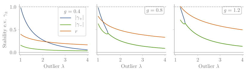
Figure 7: Stability eigenvalues $\gamma_{\pm}$ depend on the outlier $\lambda$ corresponding to a fixed point. The $\gamma_{\pm}$ are solutions to the mean field equations, fully determined by the eigenvalue $\lambda$ and the random strength $g$. The three plots corresponds to $g\in\{0.4,0.8,1.2\}$. Orange lines: radius of the bulk; any eigenvalues with smaller magnitude will not be observable, and hence not numerically testable for finite size networks. Where the absolute values of $\gamma_{\pm}$ coincide, the two form a pair of complex conjugates. Note that for $g>1$, the minimal $\lambda$ to stabilize the chaotic activity is larger than one.

In the autonomous case, $\mathbf{I}=\mathbf{0}$, the square brackets in Eq. 98 become identical, and the equation splits into a quadratic part and one of degree $K-1$. By applying the identity $\lambda=1/\langle\phi^{\prime}\rangle$, we arrive at

$$0=\left[\lambda\gamma-\mathbf{n}^{T}\!\left(\mathds{1}-\frac{J}{\lambda\gamma}\right)^{-1}\!\mathbf{m}\right]\left[\frac{\langle\phi^{\prime\prime\prime}\rangle\kappa^{2}\lambda\gamma}{(\gamma-q)(\gamma-1)}-1\right]\,.$$ (99)

The second bracket is squared in $\gamma$ and exhibits the roots

$$\gamma_{\pm} =\frac{c}{2}\pm\sqrt{\left(\frac{c}{2}\right)^{2}-q}\,,$$ (100)

with

$$c =1+q+\kappa^{2}\frac{\langle\phi^{\prime\prime\prime}\rangle}{\langle\phi^{\prime}\rangle}\,,$$ (101)

and $q=g^{2}\langle\phi^{\prime\prime}\phi+\phi^{\prime 2}\rangle$ as defined above, Eq. 84. We observe that $\gamma_{\pm}$ is entirely defined by the fixed point statistics. One can even reduce the problem to two parameters, for example the outlier $\lambda$ and the network parameter $g$ which quantifies the strength of the random connectivity. This allows to thoroughly scan the numerical values of $\gamma_{\pm}$. The results can be observed in Fig. 7. The first observation is that both $\gamma_{+}$ and $\gamma_{-}$ are always smaller than one. They hence do not destabilize the fixed point. Additionally, we can compare $\gamma_{\pm}$ to the radius of the bulk, which is given by $r=g\sqrt{\langle\phi^{\prime 2}\rangle}$ Mastrogiuseppe and Ostojic (2018). This shows that $\gamma_{-}$ is always within the bulk and hence not observable numerically.

The roots of the first bracket in Eq. 99 are identified by comparing once again with Eq. 5 which defines the outliers $\lambda$ of the spectrum at the origin. In fact, the equation is identical, but now the variable is $\lambda\gamma$. Here, $\lambda$ is the outlier corresponding to the fixed point under consideration. We hence need to fulfill $\lambda\gamma=\lambda^{\prime}$ for some $\lambda^{\prime}$ in the set of outliers. Accordingly, the solutions are given by Eq. 29 in the main text.

The case $\lambda=\lambda^{\prime}$ and hence $\gamma=1$ was omitted in the discussion above. However, one observes from Eq. 92 after insertion of $\lambda=1/\langle\phi^{\prime}\rangle$ that $\gamma=1$ would necessitate $\mathbf{n}^{T}\!\left(\mathds{1}-J/\lambda\right)^{-2}\mathbf{m}=0$. According to Eq. 5, the eigenvalues $\lambda$ are the roots of the function $f(\lambda)=\mathbf{n}^{T}\!\left(\mathds{1}\lambda-J\right)^{-1}\mathbf{m}\,-\,1$. The function has the derivative $\mathrm{d}f/\mathrm{d}\lambda=-\mathbf{n}^{T}\!\left(\mathds{1}\lambda-J\right)^{-2}\mathbf{m}$, which only vanishes if the roots have multiplicity larger than 1. Thus $\gamma=1$ is only a solution if the corresponding $\lambda$ has algebraic multiplicity larger than 1.

Appendix H Stability for rank-two perturbation

The stability of a fixed point in the case of a rank-two perturbation can be evaluated similarly to the rank-one case. One simply applies the matrix determinant lemma once more on the stability matrix. Let $\lambda=1/\langle\phi^{\prime}\rangle$ be the outlier corresponding to the fixed point under consideration. All mean field quantities will hence implicitly depend on $\lambda$, even though we omit this dependency in the notation. The quadratic equation for the stability eigenvalues $\gamma$ reads

$$0=\gamma^{2}-\gamma\mathrm{Tr}\tilde{Q}_{\gamma}+\det(\tilde{Q}_{\gamma})\,,$$ (102)

with the mean field form of the stability matrix

$$\tilde{Q}_{\gamma}=\begin{bmatrix}\mathbf{n}^{T}\!\tilde{M}_{\gamma}\mathbf{m}&\mathbf{n}^{T}\!\tilde{M}_{\gamma}\mathbf{u}\\ \mathbf{v}^{T}\!\tilde{M}_{\gamma}\mathbf{m}&\mathbf{v}^{T}\!\tilde{M}_{\gamma}\mathbf{u}\end{bmatrix}\,,$$ (103)

and $\tilde{M}_{\gamma}=R^{\prime}(\mathds{1}-JR^{\prime}/\gamma)^{-1}$. As above, Eq. 92, we have

$$\begin{split}\mathbf{a}^{T}\!\tilde{M}_{\gamma}\mathbf{b}&=\mathbf{a}^{T}\!\left(\mathds{1}-\frac{\langle\phi^{\prime}\rangle}{\gamma}J\right)^{-1}\left(\langle\phi^{\prime}\rangle\mathbf{b}+\frac{\langle\phi^{\prime\prime\prime}\rangle}{1-\frac{q}{\gamma}}\mathbf{b}^{T}\!\mathbf{x}\,\mathbf{x}\right)\\ &=\frac{1}{\lambda}\mathbf{a}^{T}M_{\lambda\gamma}\mathbf{b}\\ &\quad+\frac{\langle\phi^{\prime\prime\prime}\rangle\gamma}{(\gamma-q)(\gamma-1)}\mathbf{b}^{T}(\kappa_{1}\mathbf{m}+\kappa_{2}\mathbf{u})\\ &\qquad\times\mathbf{a}^{T}(\gamma M_{\lambda}-M_{\lambda\gamma})(\kappa_{1}\mathbf{m}+\kappa_{2}\mathbf{u})\,,\end{split}$$ (104)

for two vectors $\mathbf{a}$ and $\mathbf{b}$ and $M_{\lambda}=(\mathds{1}-J/\lambda)^{-1}$ as before, Eq. 33. The second line is valid in case of an autonomous fixed point, c.f. Eq. 99. Evaluating the terms appearing in $\tilde{Q}_{\gamma}$, we arrive at

$$\tilde{Q}_{\gamma}=\frac{1}{\lambda}\left[Q_{\lambda\gamma}+A\,\Delta Q\,\bm{\kappa}\bm{\kappa}^{t}\right]\,.$$ (105)

We abbreviated $A=\frac{\langle\phi^{\prime\prime\prime}\rangle\lambda\gamma}{(\gamma-q)(\gamma-1)}$ and $\Delta Q=\gamma Q_{\lambda}-Q_{\lambda\gamma}$. The trace and determinant are then conveniently evaluated as

$$\det(\tilde{Q}_{\gamma}) =\frac{\det(Q_{\lambda\gamma})}{\lambda^{2}}\left(1+A\bm{\kappa}^{t}(Q_{\lambda\gamma})^{-1}\Delta Q\bm{\kappa}\right)\,,$$ (106)

$$\mathrm{Tr}(\tilde{Q}_{\gamma}) =\frac{1}{\lambda}\left(\mathrm{Tr}(Q_{\lambda\gamma})+A\bm{\kappa}^{t}\Delta Q\bm{\kappa}\right)\,.$$ (107)

Inserting these expressions into the stability eigenvalue equation (102) and recalling that $\bm{\kappa}$ is an eigenvector of $Q_{\lambda}$, Eq. 35, we finally arrive at

$$0=\left[(\lambda\gamma)^{2}-\lambda\gamma\mathrm{Tr}(Q_{\lambda\gamma})+\det(Q_{\lambda\gamma})\right]\left[1-A\bm{\kappa}^{t}\bm{\kappa}\right]\,.$$ (108)

We hence arrive at the same solutions as in the case of a rank-one perturbation, Eqs. 29 and 100.

References

- Rigotti et al. (2013) Mattia Rigotti, Omri Barak, Melissa R Warden, Xiao-Jing Wang, Nathaniel D Daw, Earl K Miller, and Stefano Fusi, “The importance of mixed selectivity in complex cognitive tasks,” Nature 497, 585 (2013).
- Yang et al. (2019) Guangyu Robert Yang, Madhura R Joglekar, H Francis Song, William T Newsome, and Xiao-Jing Wang, “Task representations in neural networks trained to perform many cognitive tasks,” Nature Neuroscience 22, 297 (2019).
- Rivkind and Barak (2017) Alexander Rivkind and Omri Barak, “Local dynamics in trained recurrent neural networks,” Physical Review Letters 118, 258101 (2017).
- Mastrogiuseppe and Ostojic (2018) Francesca Mastrogiuseppe and Srdjan Ostojic, “Linking connectivity, dynamics, and computations in low-rank recurrent neural networks,” Neuron 99, 609–623 (2018).
- Tirozzi and Tsodyks (1991) B Tirozzi and M Tsodyks, “Chaos in highly diluted neural networks,” EPL (Europhysics Letters) 14, 727 (1991).
- Roudi and Latham (2007) Yasser Roudi and Peter E Latham, “A balanced memory network,” PLoS computational biology 3, e141 (2007).
- Ahmadian et al. (2015) Yashar Ahmadian, Francesco Fumarola, and Kenneth D Miller, “Properties of networks with partially structured and partially random connectivity,” Physical Review E 91, 012820 (2015).
- Ben-Yishai et al. (1995) R Ben-Yishai, R Lev Bar-Or, and H Sompolinsky, “Theory of orientation tuning in visual cortex.” Proceedings of the National Academy of Sciences 92, 3844–3848 (1995).
- Hopfield (1982) John J Hopfield, “Neural networks and physical systems with emergent collective computational abilities,” Proceedings of the National Academy of Sciences 79, 2554–2558 (1982).
- Wang (2002) Xiao-Jing Wang, “Probabilistic decision making by slow reverberation in cortical circuits,” Neuron 36, 955–968 (2002).
- Amit et al. (1985) Daniel J Amit, Hanoch Gutfreund, and Haim Sompolinsky, “Spin-glass models of neural networks,” Physical Review A 32, 1007 (1985).
- Sompolinsky et al. (1988) Haim Sompolinsky, Andrea Crisanti, and Hans-Jurgen Sommers, “Chaos in random neural networks,” Physical Review Letters 61, 259 (1988).
- Rajan et al. (2010) Kanaka Rajan, LF Abbott, and Haim Sompolinsky, “Stimulus-dependent suppression of chaos in recurrent neural networks,” Physical Review E 82, 011903 (2010).
- Brunel (2000) Nicolas Brunel, “Dynamics of sparsely connected networks of excitatory and inhibitory spiking neurons,” Journal of Computational Neuroscience 8, 183–208 (2000).
- Wainrib and Touboul (2013) Gilles Wainrib and Jonathan Touboul, “Topological and dynamical complexity of random neural networks,” Physical Review Letters 110, 118101 (2013).
- Van Vreeswijk and Sompolinsky (1996) Carl Van Vreeswijk and Haim Sompolinsky, “Chaos in neuronal networks with balanced excitatory and inhibitory activity,” Science 274, 1724–1726 (1996).
- Huang et al. (2019) Chengcheng Huang, Douglas A Ruff, Ryan Pyle, Robert Rosenbaum, Marlene R Cohen, and Brent Doiron, “Circuit models of low-dimensional shared variability in cortical networks,” Neuron 101, 337–348 (2019).
- Renart et al. (2007) Alfonso Renart, Rubén Moreno-Bote, Xiao-Jing Wang, and Néstor Parga, “Mean-driven and fluctuation-driven persistent activity in recurrent networks,” Neural computation 19, 1–46 (2007).
- Maass et al. (2002) Wolfgang Maass, Thomas Natschläger, and Henry Markram, “Real-time computing without stable states: A new framework for neural computation based on perturbations,” Neural Computation 14, 2531–2560 (2002).
- Jaeger and Haas (2004) Herbert Jaeger and Harald Haas, “Harnessing nonlinearity: Predicting chaotic systems and saving energy in wireless communication,” Science 304, 78–80 (2004).
- Sussillo and Abbott (2009) David Sussillo and Larry F Abbott, “Generating coherent patterns of activity from chaotic neural networks,” Neuron 63, 544–557 (2009).
- Enel et al. (2016) Pierre Enel, Emmanuel Procyk, René Quilodran, and Peter Ford Dominey, “Reservoir computing properties of neural dynamics in prefrontal cortex,” PLoS computational biology 12, e1004967 (2016).
- Barak et al. (2013) Omri Barak, David Sussillo, Ranulfo Romo, Misha Tsodyks, and LF Abbott, “From fixed points to chaos: three models of delayed discrimination,” Progress in neurobiology 103, 214–222 (2013).
- Ginibre (1965) Jean Ginibre, “Statistical ensembles of complex, quaternion, and real matrices,” Journal of Mathematical Physics 6, 440–449 (1965).
- Rajan and Abbott (2006) Kanaka Rajan and LF Abbott, “Eigenvalue spectra of random matrices for neural networks,” Physical Review Letters 97, 188104 (2006).
- Tao (2013) Terence Tao, “Outliers in the spectrum of iid matrices with bounded rank perturbations,” Probability Theory and Related Fields 155, 231–263 (2013).
- Harville (1998) David A Harville, Matrix algebra from a statistician’s perspective (Taylor & Francis Group, 1998).
- Logiaco et al. (2019) Laureline Logiaco, LF Abbott, and Sean Escola, “A model of flexible motor sequencing through thalamic control of cortical dynamics,” bioRxiv preprint 2019.12.17.880153 (2019).
- Beer and Barak (2019) Chen Beer and Omri Barak, “One step back, two steps forward: Interference and learning in recurrent neural networks,” Neural Computation 31, 1985–2003 (2019).
- Neri and Metz (2012) Izaak Neri and Fernando L Metz, “Spectra of sparse non-hermitian random matrices: An analytical solution,” Physical Review Letters 109, 030602 (2012).
- Neri and Metz (2016) Izaak Neri and Fernando Lucas Metz, “Eigenvalue outliers of non-hermitian random matrices with a local tree structure,” Physical Review Letters 117, 224101 (2016).
- Metz et al. (2019) Fernando Lucas Metz, Izaak Neri, and Tim Rogers, “Spectral theory of sparse non-hermitian random matrices,” Journal of Physics A: Mathematical and Theoretical (2019).
- Aljadeff et al. (2015) Johnatan Aljadeff, Merav Stern, and Tatyana Sharpee, “Transition to chaos in random networks with cell-type-specific connectivity,” Physical Review Letters 114, 088101 (2015).
- Mastrogiuseppe and Ostojic (2019) Francesca Mastrogiuseppe and Srdjan Ostojic, “A geometrical analysis of global stability in trained feedback networks,” Neural computation 31, 1139–1182 (2019).
- Rivkind et al. (2019) Alexander Rivkind, Hallel Schreier, Naama Brenner, and Omri Barak, “Scale free topology as an effective feedback system,” BioRxiv , 696575 (2019).
- Furusawa and Kaneko (2018) Chikara Furusawa and Kunihiko Kaneko, “Formation of dominant mode by evolution in biological systems,” Physical Review E 97, 042410 (2018).