PMD: A New User Distance for Recommender Systems

Abstract.

Collaborative filtering, a widely-used recommendation technique, predicts a user’s preference by aggregating the ratings from similar users. Traditional similarity measures utilize ratings of only co-rated items while computing similarity between a pair of users. As a result, these measures cannot fully utilize the rating information and are not suitable for real world sparse data. To solve these issues, we propose a novel user distance measure named Preference Mover’s Distance (PMD) which makes full use of all ratings made by each user. Our proposed PMD can properly measure the distance between a pair of users even if they have no co-rated items. We show that this measure can be cast as an instance of the Earth Mover’s Distance, a well-studied transportation problem for which several highly efficient solvers have been developed. Experimental results show that PMD can help achieve superior recommendation accuracy than state-of-the-art methods, especially when training data is very sparse.

1. Introduction

Collaborative filtering (CF) is one of the most widely-used user-centric recommendation techniques in practice (Guo et al., 2013; Zheng et al., 2010). For a specific user, CF recommends items according to the preference of similar users. User similarity plays an important role in CF, including both memory-based (Zheng et al., 2010) and model-based (Ma et al., 2011) approaches. First, it serves as a criterion to select a group of most similar users whose ratings will form the basis of recommendations. Second, it is also used to weigh the users so that more similar users will have greater impact on recommendations.

Some traditional similarity measures, such as Cosine (COS) (Breese et al., 1998), Persons Correlation Coefficient (PCC) (Breese et al., 1998) and so on, have been widely used in CF to evaluate similarity (Wang et al., 2017; Desrosiers and Karypis, 2011). However, They only consider ratings on the co-rated items (Patra et al., 2015; Wang et al., 2017), which may not represent the taste of a user properly. The reason is that the information is lost while ignoring the ratings on the non-co-rated items (Patra et al., 2015; Wang et al., 2017). Figure 1 shows examples of co-rated items. Therefore, these measures perform poorly if there are no sufficient numbers of co-rated items and thus are not suitable for real world sparse data (Patra et al., 2015; Wang et al., 2017), because the more sparse the data the less likely the co-rated items can exist. Moreover, these measures are not applicable when there are no co-rated items at all.

To measure user similarity more accurately, one should make full use of all ratings of each user. However, computing user similarity based on the ratings of two different sets of items is challenging—let’s imagine an extreme case that user A and B rate completely different items. Therefore, it requires additional information to build the connections between their ratings. We consider the similarity among items to establish the connection between ratings from different items. Item similarity is actually more general than “co-rated”, because “co-rated” means the users rate the same items and same is also one kind of similarity. We proposed to compute user similarity by assuming: if two users have similar opinions on similar items, then their tastes are similar. Our assumption differs from traditional methods (Breese et al., 1998) in that we compare user opinions based on similar items instead of just “co-rated” ones.

We propose the Preference Mover’s Distance (PMD) which fully utilizes all ratings made by each user and can evaluate user similarity even in the absence of co-rated items. PMD can guarantee that if user A and B are both similar to C, then A and B should also be similar, as implied by triangle inequality. The optimization problem of computing PMD reduces to a special case of the Earth Mover’s Distance (Monge, 1781; Rubner et al., 1998; Wolsey and Nemhauser, 2014), a well-studied transportation problem for which fast specialized solvers (Ling and Okada, 2007; Pele and Werman, 2009) has been developed. Experimental results show that PMD can help achieve superior recommendation accuracy over state-of-the-art measures, especially when training data is sparse.

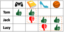
Figure 1. Examples of co-rated items. Jack and Tom “‘co-rated” the book while Jack and Lucy “co-rated” the high-heeled shoes and the basketball. Tom and Lucy have no co-rated items.

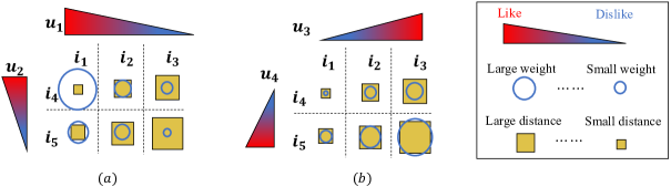
Figure 2. An illustration of our basic philosophy to evaluate user distance. The bigger the square the larger the item distance $d(i,j)$, e.g. $i_{1}$ and $i_{4}$ are similar while $i_{3}$ and $i_{5}$ are dissimilar. The bigger the circle the larger the weight $\mathbf{W}_{u,v}(i,j)$. In subfigure (a), $\mathcal{I}_{u1}=\{i_{1},i_{2},i_{3}\}$, $\mathbf{p}_{u1}(i_{1})>\mathbf{p}_{u1}(i_{2})>\mathbf{p}_{u1}(i_{3})$; $\mathcal{I}_{u2}=\{i_{4},i_{5}\}$, $\mathbf{p}_{u2}(i_{4})>\mathbf{p}_{u2}(i_{5})$. Since $u_{1}$ and $u_{2}$ like similar items, such as $i_{1}$ and $i_{4}$, we give their distances large weights such that $D(u_{1},u_{2})$ is small. In subfigure (b), since $u_{3}$ and $u_{4}$ like dissimilar items, such as $i_{3}$ and $i_{5}$, we give their distances large weights such that $D(u_{3},u_{4})$ is large.

2. Related Work

COS and PCC are two most classic and widely-used user similarity measures. Afterwards, numerous variants of COS and PCC have been proposed, such as Adjusted Cosine  (Sarwar et al., 2001), Constrained PCC (Shardanand and Maes, 1995), Weighted PCC (Ma et al., 2007), Sigmoid PCC (Jamali and Ester, 2009), etc. However, they are not motivated for handling the “co-rated item” issue and still suffers from the problem. Apart from them, some other measures, such as Jaccard (Koutrika et al., 2009), MSD (Shardanand and Maes, 1995), JMSD (Bobadilla et al., 2010), URP (Liu et al., 2014), NHSM (Liu et al., 2014), PIP (Ahn, 2008) and BS (Guo et al., 2013) also suffers from the “co-rated item” issue (Al-bashiri et al., 2017). Although some of them, such as Jaccard and URP consider all ratings of each user, they are inefficient in use of the rating information. For example, Jaccard only uses the number of items while omits the specific rating values; URP only uses the mean and variance of rating values. Moreover, they all fail when there are no co-rated items at all.

The most relevant works to us are BCF (Patra et al., 2015) and HUSM (Wang et al., 2017), which predict user similarity by utilizing all ratings of each user and also item similarities. Although BCF and HUSM can partially solve the “co-rated item” issue and show good performance on sparse data, they also have drawbacks and sometimes give counter-intuitive results, as illustrated in section 3 and section 4.1 respectively. For your convenience, please refer to the supplementary material for the definitions of these previous methods.

3. The Proposed Similarity Measure

Problem definition. Let $\mathcal{U}$ be a set of $m$ users, and $\mathcal{I}$ a set of $n$ items. The user-item interaction matrix is denoted by $\mathbf{R}\in\mathbb{R}^{m\times n}$ with $\mathbf{R}(u,i)\geq 0$ the rating of user $u$ given to item $i$. For user $u\in\mathcal{U}$, his rated items are $\mathcal{I}_{u}\subset\mathcal{I}$. Usually $\mathbf{R}$ is a partially observed matrix and highly sparse. $d(i,j)\geq 0$ denotes the distance between item $i$ and $j$, which evaluates the similarity between them. The smaller $d(i,j)$ the more similar $i$ and $j$. We can derive $d(i,j)$ from ratings on items (Patra et al., 2015; Wang et al., 2017) or content information (Yao and Harper, 2018), such as item tags, comments, etc. In this paper, we assume $d(i,j)$ are given. How to construct high-quality item distances is beyond the scope of this paper. We are interested in computing the distance between any pair of users in $\mathcal{U}$ given $\mathbf{R}$ and $d$. Then user similarity can be easily derived from user distance, since they are negatively correlated.

User preference representation. Let $\Sigma_{k}=\{\mathbf{p}\in[0,1]^{k}\;|\;\braket{\mathbf{p},\mathds{1}}=1\}$ denotes a $(k-1)$-dimensional simplex. We model a user $u$’s preference as a probabilistic distribution $\mathbf{p}_{u}\in\Sigma_{|\mathcal{I}_{u}|}$ on $\mathcal{I}_{u}$, where $\mathbf{p}_{u}(i)$ represents how much the user $u$ likes item $i$. The larger $\mathbf{p}_{u}(i)$ the more $u$ likes $i$. In practice, the ground truth of $\mathbf{p}_{u}$ is unobserved and we estimate it by normalizing $u$’s ratings on $\mathcal{I}_{u}$, i.e. $\mathbf{p}_{u}(i)\approx\frac{\mathbf{R}(u,i)}{\sum_{j\in\mathcal{I}_{u}}\mathbf{R}(u,j)}$ for $i\in\mathcal{I}_{u}$.

User preference distance. Ratings and rated items both reflect the difference between a pair of users. Hence, we consider these two different types of information while modeling user distance. Specifically, we model the distance between user $u$ and $v$, denoted by $D(u,v)$, as the weighted average of the distances among their rated items, i.e.

(1) $$\sum_{i\in\mathcal{I}_{u}}\sum_{j\in\mathcal{I}_{v}}\mathbf{W}_{u,v}(i,j)d(i,j),$$

where $\mathbf{W}_{u,v}(i,j)\geq 0$ is the weight of $d(i,j)$ and $\sum_{i\in\mathcal{I}_{u}}\sum_{j\in\mathcal{I}_{v}}\mathbf{W}_{u,v}(i,j)\\ =1$. The weights $\mathbf{W}_{u,v}$ embody the difference among the ratings of $u$ and $v$ such that $D(u,v)$ is small if $u$ and $v$ like (give high ratings to) similar items. Our strategy to construct such a $\mathbf{W}_{u,v}$ is: If $u$ and $v$ like similar items, the $\mathbf{W}_{u,v}(i,j)$ of similar items, whose $d(i,j)$ are small, should be large such that the resulting user distance is small; If $u$ and $v$ like dissimilar items, the $\mathbf{W}_{u,v}(i,j)$ of dissimilar items, whose $d(i,j)$ are large, should be large such that the resulting user distance is large. Figure 2 briefly illustrates this strategy. To summarize, we find the strategy just makes the mass of $\mathbf{W}_{u,v}$ concentrate on the item pairs that are ‘liked’ by both users, as can be noticed in Figure 2a and 2b. Hence, we implement this strategy by making the marginal distribution of $\mathbf{W}_{u,v}$ follow $\mathbf{p}_{u}$ and $\mathbf{p}_{v}$ respectively, i.e. $\mathbf{W}_{u,v}\in U(\mathbf{p}_{u},\mathbf{p}_{v})$, where

(2) $$U(\mathbf{p}_{u},\mathbf{p}_{v}):= \left\{\mathbf{W}_{u,v}\in[0,1]^{|\mathcal{I}_{u}|\times|\mathcal{I}_{v}|}\;|\;\mathbf{W}_{u,v}\mathds{1}=\mathbf{p}_{u},\mathbf{W}_{u,v}^{T}\mathds{1}=\mathbf{p}_{v}\right\}.$$

However, there are many $\mathbf{W}_{u,v}$ that satisfy $\mathbf{W}_{u,v}\in U(\mathbf{p}_{u},\mathbf{p}_{v})$, which results in the user distance value indeterminate. Therefore, we define the user distance as the smallest one among all possible values:

(3) $$D(u,v):=\min_{\mathbf{W}_{u,v}\in U(\mathbf{p}_{u},\mathbf{p}_{v})}\sum_{i\in\mathcal{I}_{u}}\sum_{j\in\mathcal{I}_{v}}\mathbf{W}_{u,v}(i,j)d(i,j),$$

A benefit of taking minimum in formula (3) is that the resulting distance is a metric as long as $d$ is a metric (Rubner et al., 1998).

	Iron Man	Bat Man	Spider Man	Titanic	Casablanca
$u_{1}$	5	—	2	3	—
$u_{2}$	—	5	2	3	—
$u_{3}$	—	—	2	3	5
$u_{4}$	5	5	5	—	—
$u_{5}$	—	—	—	5	—
$u_{6}$	—	—	—	—	5

(a) Users’ ratings on five movies.

	Iron Man	Bat Man	Spider Man	Titanic	Casablanca
Iron Man	1	0.8	0.8	0.3	0.3
Bat Man	0.8	1	0.8	0.3	0.3
Spider Man	0.8	0.8	1	0.3	0.3
Titanic	0.3	0.3	0.3	1	0.8
Casablanca	0.3	0.3	0.3	0.8	1

(b) The similarity matrix among movies. For PMD, we derive $d(i,j)$ by $d(i,j):=arccos(similarity(i,j))$.

Case	Similarity between	COS	PCC	$1-$MSD	Jaccard	URP	JMSD	NHSM	BCF	N-BCF	HUSM	N-HUSM	$1-$PMD
(1) Co-rated items exist	$u_{1}$ & $u_{2}$	1	1	1	0.5	0.5	0.5	0.0769	3.277*	0.809*	0.197*	0.0218*	0.892*
	$u_{2}$ & $u_{3}$	1	1	1	0.5	0.5	0.5	0.0769	2.444*	0.716*	0.157*	0.0175*	0.633*
(2) No co- rated items	$u_{4}$ & $u_{5}$	—	—	—	0	0.5	—	—	0.9	0.3*	0.0552	0.0184*	0.3*
	$u_{5}$ & $u_{6}$	—	—	—	0	0.5	—	—	0.8	0.8*	0.0491	0.0491*	0.8*

(c) User similarity computed by various methods. Since MSD and PMD are distance measures, we convert them to similarity values by $similarity:=1-distance$ for easy comparison. Desirable values are followed by a ‘*’.

(d) Toy examples of user similarity computed by various methods.

The optimization in formula (3) is in coincidence with a special case of the earth mover’s distance metric (EMD) (Monge, 1781; Rubner et al., 1998; Wolsey and Nemhauser, 2014), a well studied transportation problem for which specialized solvers have been developed (Ling and Okada, 2007; Pele and Werman, 2009). To highlight this connection we refer to our proposed user distance as the Preference Mover’s Distance (PMD).

Remark 1: Comparing with BCF and HUSM. BCF and HUSM also have a similar basic form of $\sum_{i\in\mathcal{I}_{u}}\sum_{j\in\mathcal{I}_{v}}Sim_{rating}(r_{ui},r_{vj})$ Simitem(i,j), where $Sim_{rating}(r_{ui},r_{vj})$ evaluates rating similarity and $Sim_{item}(i,j)$ represents item similarity. Nevertheless, (1) They don’t normalize the number of terms in the summation. Therefore, the resulting user similarity can grow linearly w.r.t. the number of terms (item pairs) in the sum. However, the number of item pairs do not necessarily imply user similarity. Thus, the resulting similarity values could be misleading. In contrast, $\mathbf{W}_{u,v}$ serves as a natural normalization for PMD. (2) Even if we consider their normalized versions, BCF and HUSM derive each $Sim_{rating}(r_{ui},r_{vj})$ independently and heuristically, while we derive $\mathbf{W}_{u,v}$ through optimization. As a result, PMD satisfies triangle inequality, while BCF and HUSM do not have equivalent properties. Triangle inequality limits each distance value to a reasonable range which is defined by other distance values. Consequently, PMD can guarantee that if user A and B are both similar to C, then A and B are also similar to each other. Thus, we can weigh the neighbors more reasonably according to the distance values given by PMD.

4. Experiments

In this section, we first use several case studies to give the reader an insight into the superiority of PMD over other measures, then we compare the recommendation accuracy of these measures on two real world data sets.

Comparison Measures. COS, PCC and MSD are three classic user similarity measures. Jaccard, URP, JMSD, NHSM, BCF, HUSM are five representatives that try to use all ratings of each user to evaluate user similarity. To study how normalization influence the performance of BCF and HUSM, we also consider their normalized versions which normalize the number of item pairs: $\frac{\sum_{i\in\mathcal{I}_{u}}\sum_{j\in\mathcal{I}_{v}}Sim_{rating}(r_{ui},r_{vj})\cdot{\\ }Sim_{item}(i,j)}{|\mathcal{I}_{u}|\times|\mathcal{I}_{v}|}$. The resulting similarity measures are named as N-BCF and N-HUSM respectively.

4.1. Case Study

We illustrate by examples the differences among the similarity values computed by various methods under the two cases: (1) there exist co-rated items and (2) there are no co-rated items. In Table 1(a), the ratings of six users on five movies are presented. User $u_{1}$, $u_{2}$ and $u_{3}$ are used to simulate case (1) while user $u_{3}$, $u_{4}$ and $u_{5}$ to simulate case (2). The five movies consist of three sci-fi movies and two romantic movies. As BCF, HUSM and PMD require item similarity/distance for computation, we assume we know the ground truth of movie similarities, as shown in 1(b). The similarity values computed by various methods are shown in 3.

In Case (1), although $u_{1}$, $u_{2}$ and $u_{3}$ all give exactly the same ratings to their co-rated items, $u_{1}$ and $u_{2}$’s high ratings are both on sci-fi movies while $u_{3}$’s high ratings on romantic movies. This implies that $u_{1}$ and $u_{2}$ like sci-fi more than romance while $u_{3}$ loves romance more. Therefore, $u_{1}$ and $u_{2}$ should be more similar than $u_{2}$ and $u_{3}$. However, COS, PCC, MSD, Jaccard, URP, JMSD and NHSM all give $Sim(u_{1},u_{2})=Sim(u_{2},u_{3})$, which is counter-intuitive. The reason is that COS, PCC, MSD only consider ratings on co-rated movies; Jaccard omits the exact rating values; and URP only considers mean and variance of rating values. JMSD and NHSM also fail in this case because their ability of using all ratings is granted by Jaccard or URP. The only successful measures in this case are BCF, N-BCF, HUSM, N-HUSM and our PMD, because they make full use of all rating information.

In Case (2), $u_{3}$, $u_{4}$ and $u_{5}$ have no co-rated items at all. However, $u_{3}$ and $u_{4}$’s high ratings are both on sci-fi movies while $u_{5}$’s high ratings on romantic movies. Like Case (1), $u_{3}$ and $u_{4}$ should be more similar than $u_{4}$ and $u_{5}$. However, COS, PCC, MSD, JMSD and NHSM all can’t work in this case because they must use the ratings on co-rated items. Jaccard gives 0 as long as there are no co-rated items. URP again gives identical similarity values for the same reason discussed in Case (1). Although BCF and HUSM utilize all rating information, they give a misleading result of $Sim(u_{4},u_{5})>Sim(u_{5},u_{6})$ while the desired one should be $Sim(u_{4},u_{5})<Sim(u_{5},u_{6})$. This is because there are more item pairs between $u_{4}$ and $u_{5}$ than $u_{5}$ and $u_{6}$ and they didn’t normalize the number of item pairs. By contrast, N-BCF and N-HUSM works well because of normalization. Our PMD again performs well even in the absence of co-rated items and is not misled by the number of item pairs.

Although N-BCF, N-HUSM and PMD can all judge user similarity correctly in Case (1) and (2), PMD generates more reasonable distance values as discussed in Remark 1. In the next section, we conduct experiments to further justify this point.

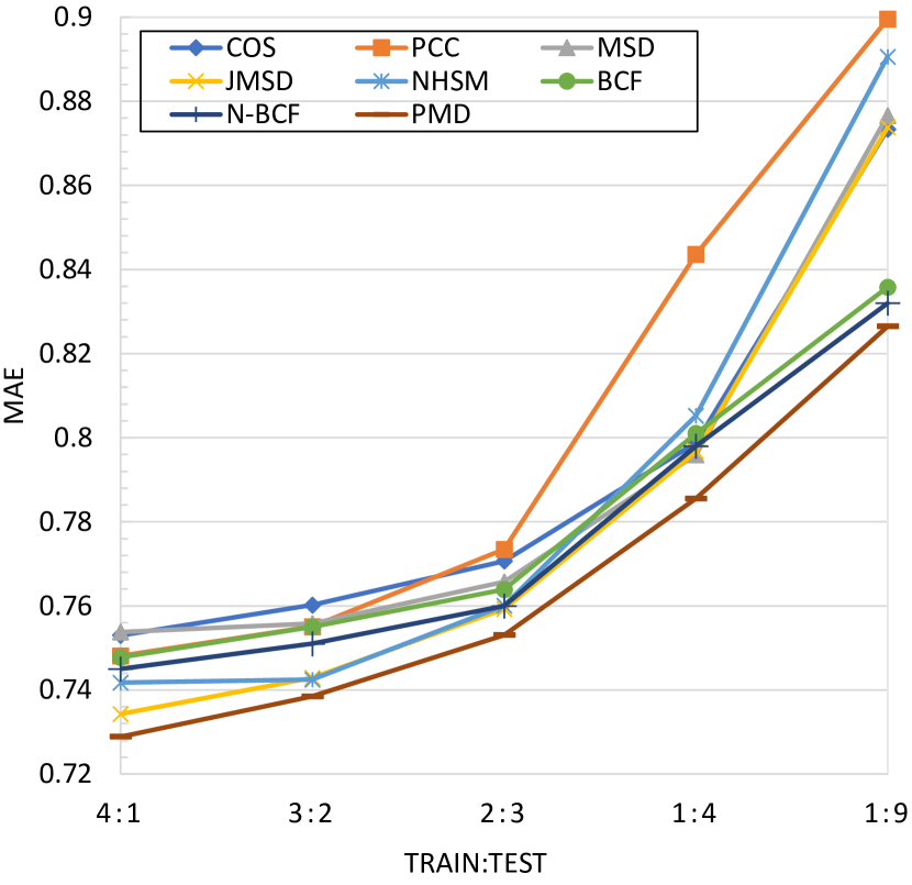
(a) train:test from 4:1 to 1:9; K=40.

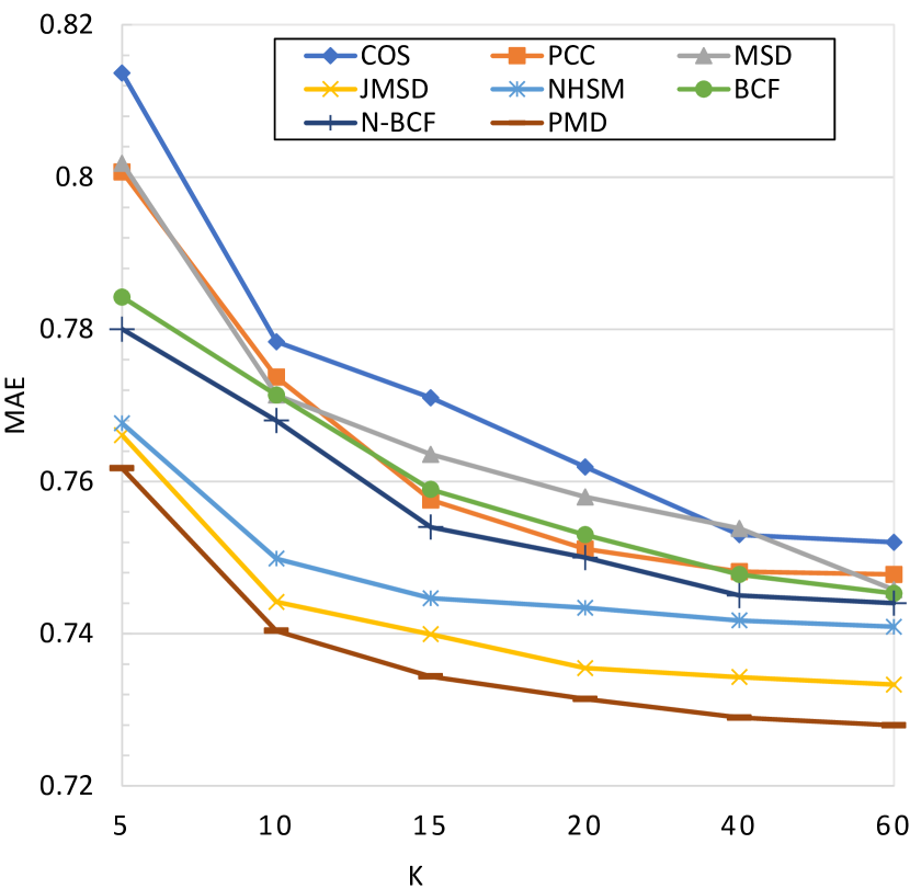
(b) train:test=4:1; K from 5 to 60.

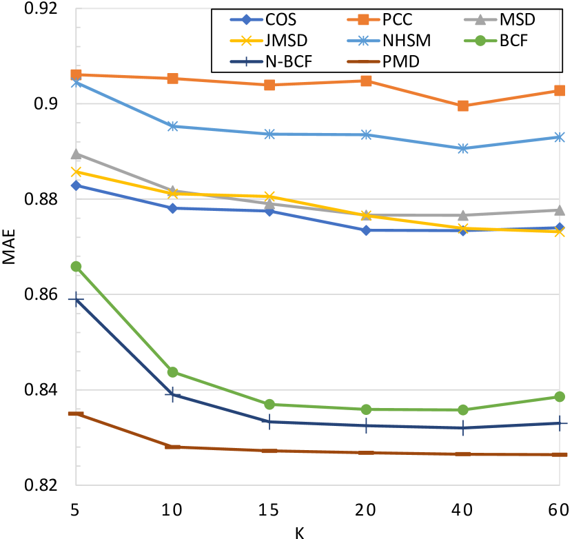
(c) train:test=1:9; K from 5 to 60.

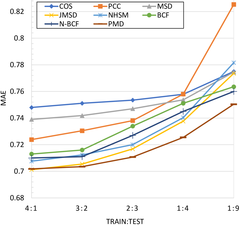
(d) train:test from 4:1 to 1:9; K=40.

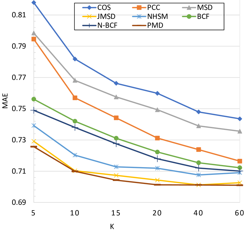
(e) train:test=4:1; K from 4 to 60.

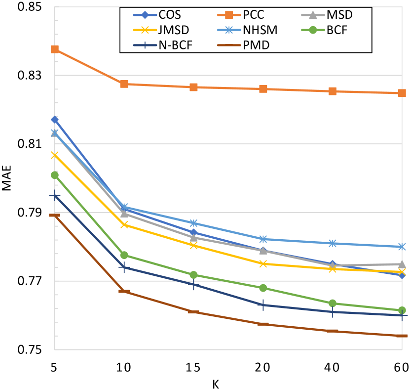
(f) train:test=1:9; K from 4 to 60.

Figure 3. MAE of comparative approaches on MovieLens- 100K (a-c) and MovieLens-1M (d-f). Experimental settings corresponding to each subfigure are summarized in their subtitles in a format of ”train:test ratio; K.”

4.2. Experiments on Real World Data Set.

We evaluate the recommendation performance of various similarity measures by cross validation on two well-known datasets: MovieLens-100k and MovieLens-1M. We perform each experiment five times and take the average test performance as the final results. We apply the K-NN approach to select a group of similar users whose ranking are in the top K according to user similarity/distance. The ratings of selected similar users are aggregated to predict items’ ratings by a mean-centring approach (Desrosiers and Karypis, 2011). We use mean absolute error (MAE) to evaluate recommendation performance. Lower MAE indicates better accuracy. While our experiments use memory-based CF, we emphasize that user distance computation is equally relevant to model-based methods, including those based on matrix factorization such as (2011).

Item similarity We construct item similarity matrix by Tag-genomes  (Vig et al., 2012) of movielens.org. For the sake of fairness, the same item similarity matrix is used in PMD, BCF, N-BCF, HUSM and N-HUSM. We compute the cosine value of the tag-genomes of two movies as the similarity between them, which is a well-developed method to evaluate movie similarities (Vig et al., 2012; Yao and Harper, 2018). For PMD, it needs to convert item similarity to item distance and we define the item distance as $Distance:=arccos(Similarity)$, which is a metric. There are of course other ways (Yao and Harper, 2018) to construct item similarity matrix. We use tag-genome because it gives item similarity of high quality (Yao and Harper, 2018). How to construct high quality item similarities is beyond the scope of this paper.

Experimental Protocol. To test the performance of PMD and its robustness to data sparsity, we vary the train to test ratio from 4:1 to 1:9, during which the training data become more and more sparse. In addition, in order to study how parameter K affects the performance of various methods, we vary K from 5 to 60 with train:test ratio fixed to specific values.

Results. Experimental results are summarized in Figure 3 .

Figure 2(a) and 2(d) shows how different levels of data sparsity affects the performance of various methods when K is fixed to 40. PMD outperforms all competitive methods on all train to test ratios. In the two figures, the performance of all measures degrade as the train to test ratio deceases, because training data is becoming more and more sparse. Specifically, the performance gaps between our method and those of COS, PCC, MSD, JMSD and NHSM become larger and larger as the training data grows more and more sparse. This is probably because when data goes sparse, co-rated items hardly exist for most user pairs, making the resulting user similarity misleading or uncomputable for these methods. By contrast, PMD can compute similarity properly no matter co-rated items exist or not. When train to test ratio is 1:9, PMD can significantly advance these measures, which is also notable in 2(c) and 2(f). BCF and N-BCF shows a similar trend as PMD and beats all previous methods when data is highly sparse (e.g. train:test=1:9), probably because they also make full use of all ratings of each user. N-BCF performs slightly better than BCF possibly because of normalization. However, PMD always performs better than BCF and N-BCF, possibly because PMD has a natural normalization strategy and can weigh the neighbors more reasonably as discussed in Remark 1.

Figure 2(b) and 2(e) show how K affects the performance when train to test ratio is fixed to 4:1. As the number of neighbors increases from 5 to 60, the performance of all methods improves. This may be because more information are incorporated and noise is averaged out. PMD outperforms others consistently when K varies. This again shows PMD can give more accurate user similarity than other methods.

Similarly, figure 2(c) and 2(f) show how K affects the performance when the train to test ratio is 1:9, which means the training data is even more sparse. Our method shows significant advantage over the competitive baselines. In 2(c), the performance of COS, PCC, MSD, JMSD and NHSM are nearly constant as K varies and stay at a low accuracy level. This may be because many user pairs have no co-rated items and consequently the corresponding similarity is uncomputable when training data is highly sparse. Thus, for many users, the number of neighbors with an effective similarity value is often less than the parameter K, resulting the performance unchanged when K increases.

References

- (1)
- Ahn (2008) Hyung Jun Ahn. 2008. A new similarity measure for collaborative filtering to alleviate the new user cold-starting problem. Information Sciences 178, 1 (2008), 37–51.
- Al-bashiri et al. (2017) Hael Al-bashiri, Mansoor Abdullateef Abdulgabber, Awanis Romli, and Fadhl Hujainah. 2017. Collaborative Filtering Similarity Measures: Revisiting. In Proceedings of the International Conference on Advances in Image Processing. ACM, 195–200.
- Bobadilla et al. (2010) Jesús Bobadilla, Francisco Serradilla, and Jesus Bernal. 2010. A new collaborative filtering metric that improves the behavior of recommender systems. Knowledge-Based Systems 23, 6 (2010), 520–528.
- Breese et al. (1998) John S Breese, David Heckerman, and Carl Kadie. 1998. Empirical analysis of predictive algorithms for collaborative filtering. In Proceedings of the Fourteenth conference on Uncertainty in artificial intelligence. Morgan Kaufmann Publishers Inc., 43–52.
- Desrosiers and Karypis (2011) Christian Desrosiers and George Karypis. 2011. A comprehensive survey of neighborhood-based recommendation methods. In Recommender systems handbook. Springer, 107–144.
- Guo et al. (2013) Guibing Guo, Jie Zhang, and Neil Yorke-Smith. 2013. A novel bayesian similarity measure for recommender systems. In Twenty-Third International Joint Conference on Artificial Intelligence.
- Jamali and Ester (2009) Mohsen Jamali and Martin Ester. 2009. Trustwalker: a random walk model for combining trust-based and item-based recommendation. In Proceedings of the 15th ACM SIGKDD international conference on Knowledge discovery and data mining. ACM, 397–406.
- Koutrika et al. (2009) Georgia Koutrika, Benjamin Bercovitz, and Hector Garcia-Molina. 2009. FlexRecs: expressing and combining flexible recommendations. In Proceedings of the 2009 ACM SIGMOD International Conference on Management of data. ACM, 745–758.
- Ling and Okada (2007) Haibin Ling and Kazunori Okada. 2007. An efficient earth mover’s distance algorithm for robust histogram comparison. IEEE transactions on pattern analysis and machine intelligence 29, 5 (2007), 840–853.
- Liu et al. (2014) Haifeng Liu, Zheng Hu, Ahmad Mian, Hui Tian, and Xuzhen Zhu. 2014. A new user similarity model to improve the accuracy of collaborative filtering. Knowledge-Based Systems 56 (2014), 156–166.
- Ma et al. (2007) Hao Ma, Irwin King, and Michael R Lyu. 2007. Effective missing data prediction for collaborative filtering. In Proceedings of the 30th annual international ACM SIGIR conference on Research and development in information retrieval. ACM, 39–46.
- Ma et al. (2011) Hao Ma, Dengyong Zhou, Chao Liu, Michael R Lyu, and Irwin King. 2011. Recommender systems with social regularization. In Proceedings of the fourth ACM international conference on Web search and data mining. ACM, 287–296.
- Monge (1781) Gaspard Monge. 1781. Mémoire sur la théorie des déblais et des remblais. Histoire de l’Académie royale des sciences de Paris (1781).
- Patra et al. (2015) Bidyut Kr Patra, Raimo Launonen, Ville Ollikainen, and Sukumar Nandi. 2015. A new similarity measure using Bhattacharyya coefficient for collaborative filtering in sparse data. Knowledge-Based Systems 82 (2015), 163–177.
- Pele and Werman (2009) Ofir Pele and Michael Werman. 2009. Fast and robust earth mover’s distances. In 2009 IEEE 12th International Conference on Computer Vision. IEEE, 460–467.
- Rubner et al. (1998) Yossi Rubner, Carlo Tomasi, and Leonidas J. Guibas. 1998. A metric for distributions with applications to image databases. In Sixth International Conference on Computer Vision (IEEE Cat. No.98CH36271). 59–66.
- Sarwar et al. (2001) Badrul Munir Sarwar, George Karypis, Joseph A Konstan, John Riedl, et al. 2001. Item-based collaborative filtering recommendation algorithms. Www 1 (2001), 285–295.
- Shardanand and Maes (1995) Upendra Shardanand and Pattie Maes. 1995. Social information filtering: Algorithms for automating” word of mouth”. In Chi, Vol. 95. Citeseer, 210–217.
- Vig et al. (2012) Jesse Vig, Shilad Sen, and John Riedl. 2012. The tag genome: Encoding community knowledge to support novel interaction. ACM Transactions on Interactive Intelligent Systems (TiiS) 2, 3 (2012), 13.
- Wang et al. (2017) Yong Wang, Jiangzhou Deng, Jerry Gao, and Pu Zhang. 2017. A hybrid user similarity model for collaborative filtering. Information Sciences 418 (2017), 102–118.
- Wolsey and Nemhauser (2014) Laurence A Wolsey and George L Nemhauser. 2014. Integer and combinatorial optimization. John Wiley & Sons.
- Yao and Harper (2018) Yuan Yao and F Maxwell Harper. 2018. Judging similarity: a user-centric study of related item recommendations. In Proceedings of the 12th ACM Conference on Recommender Systems. ACM, 288–296.
- Zheng et al. (2010) Vincent W Zheng, Bin Cao, Yu Zheng, Xing Xie, and Qiang Yang. 2010. Collaborative filtering meets mobile recommendation: A user-centered approach. In Twenty-Fourth AAAI Conference on Artificial Intelligence.