The Hartree equation with a constant magnetic field: Well-posedness theory

Abstract.

We consider the Hartree equation for infinitely many electrons with a constant external magnetic field. For the system, we show a local well-posedness result when the initial data is the pertubation of a Fermi sea, which is a non-trace class stationary solution to the system. In this case, the one particle Hamiltonian is the Pauli operator, which possesses distinct properties from the Laplace operator, for example, it has a discrete spectrum and infinite-dimensional eigenspaces. The new ingredient is that we use the Fourier-Wigner transform and the asymptotic properties of associated Laguerre polynomials to derive a collapsing estimate, by which we establish the local well-posedness result.

1. Introduction

For a system of $N$ electrons moving in a constant magnetic field $B=(0,0,b)$, $(b>0)$, the Hamiltonian is described by

(1) $$\hat{\mathcal{H}}_{N}=\sum_{j=1}^{N}h_{j}+\sum_{j>k}^{N}w\left(x_{j}-x_{k}\right),\quad x_{j}\in\mathbb{R}^{3},$$

and the Schrödinger equation is

(2) $$i\,\partial_{t}\Psi_{N}(t,x_{1},x_{2},\ldots,x_{N})=\hat{\mathcal{H}}_{N}\Psi_{N}(t,x_{1},x_{2},\ldots,x_{N}),\quad\Psi_{N}(t=0)=\Psi_{N,0}\in\wedge^{N}L^{2}\left(\mathbb{R}^{3},\mathbb{C}^{2}\right),$$

where $h=\left(\sigma\cdot(-i\nabla-A)\right)^{2}$ is the Pauli operator

1. $\sigma=(\sigma_{1},\sigma_{2},\sigma_{3})$ are Pauli matrices ;

2. $\displaystyle A=-\frac{b}{2}\left(x^{2},-x^{1},0\right)$ is the vector potential of the field $\mathbf{B}=\nabla\times A$,

$h_{j}$ means $h$ acts on the variable $x_{j}$ (the $j$-th electron) and $w$ is the pairwise interaction potential. By the Pauli exclusion principle, $\Psi_{N}$ is in the space $\wedge^{N}L^{2}\left(\mathbb{R}^{3},\mathbb{C}^{2}\right)$ of anti-symmetric functions. A direct computation shows

$$h=\begin{pmatrix}\left(-i\nabla-A\right)^{2}&0\\ 0&\left(-i\nabla-A\right)^{2}\end{pmatrix}-\sigma\cdot\mathbf{B},$$

while $\sigma\cdot\mathbf{B}=\begin{pmatrix}b&0\\ 0&-b\end{pmatrix}$ is harmless for the analysis of the system. For simplicity, we consider the scalar case, i.e. $h=\left(-i\nabla-A\right)^{2}$.

The initial data $\Psi_{N,0}$ is set to be a Slater determinant

$$\Psi_{N,0}(x_{1},x_{2},\ldots,x_{N}) =\psi_{1,0}\wedge\psi_{2,0}\wedge\cdots\wedge\psi_{N,0}(x_{1},\ldots,x_{N})$$

$$:=\frac{1}{\sqrt{N!}}\sum_{\pi\in S_{N}}sgn(\pi)\psi_{1,0}(x_{\pi(1)})\psi_{2,0}(x_{\pi(2)})\cdots\psi_{N,0}(x_{\pi(N)})$$

with a family of $N$ orthonormal orbitals $\{\psi_{j,0}\}_{j=1}^{N}$ in $L^{2}(\mathbb{R}^{3})$ ($sgn(\pi)$ denotes the sign of the permutation $\pi\in S_{N}$). $\Psi_{N,0}$ is presumed as an approximation to the ground state of $\hat{\mathcal{H}}_{N}$. The total energy of Equation (2) is $\left\langle\Psi_{N},\hat{\mathcal{H}}_{N}\Psi_{N}\right\rangle$. At the initial time $t=0$, a direct computation shows that the energy is in the following form

(3) $$\sum_{j=1}^{N}\left\langle\psi_{j,0},h\psi_{j,0}\right\rangle+\frac{1}{2}\int_{\mathbb{R}^{3}\times\mathbb{R}^{3}}\left(\sum_{j=1}^{N}|\psi_{j,0}|^{2}\right)(x)w(x-y)\left(\sum_{j=1}^{N}|\psi_{j,0}|^{2}\right)(y)\,dxdy$$

$$-\frac{1}{2}\int_{\mathbb{R}^{3}\times\mathbb{R}^{3}}\left(\sum_{j=1}^{N}\psi_{j,0}(x)\bar{\psi}_{j,0}(y)\right)^{2}w(x-y)\,dxdy.$$

After the time evolution, $\Psi_{N}$ may not necessarily stay as a Slater determinant. Instead, one might expect that in an appropriate sense,

$$\Psi_{N}(t,x_{1},\ldots,x_{N})\approx\left(\psi_{1}(t)\wedge\psi_{2}(t)\wedge\cdots\wedge\psi_{N}(t)\right)(t,x_{1},\ldots,x_{N}),$$

for short time. While $\psi_{j}(t)$ is described by the following Hartree-Fock equations, for $j=1,\ldots,N$,

(6) $$\left\{\begin{array}[]{l}\displaystyle i\,\partial_{t}\psi_{j}(t,x)=\left(h+\rho_{t}*w-X\right)\psi_{j}(t,x),\\ \displaystyle\psi_{j}(0,x)=\phi_{j,0}(x),\quad\psi_{j,0}\in L^{2}\left(\mathbb{R}^{3}\right),\end{array}\right.t\in\mathbb{R},\ x\in\mathbb{R}^{3}.$$

where $\rho_{t}(x)$ is the particle density

$$\rho_{t}(x)=\sum_{k=1}^{N}\left|\psi_{k}\right|^{2}(t,x),$$

$\rho_{t}*w$ denotes the usual convolution

$$\left(\rho_{t}*w\right)(x):=\int_{\mathbb{R}^{3}}\rho_{t}(x-y)w(y)\,dy,$$

and $X$ is the integral operator with kernel

$$X(t,x,y)=\sum_{k=1}^{N}w(x-y)\psi_{k}(t,x)\bar{\psi}_{k}(t,y).$$

$\{\psi_{j}(t,x)\}_{j=1}^{N}$ remains an orthonormal set as long as Equations (6) are well-posed. Equations (6) come with a total energy

$$\sum_{j=1}^{N}\left\langle\psi_{j},h\psi_{j}\right\rangle+\frac{1}{2}\int_{\mathbb{R}^{3}\times\mathbb{R}^{3}}\rho_{t}(x)w(x-y)\rho_{t}(y)\,dxdy-\frac{1}{2}\int_{\mathbb{R}^{3}\times\mathbb{R}^{3}}\left(\sum_{j=1}^{N}\psi_{j}(x)\bar{\psi}_{j}(y)\right)^{2}w(x-y)\,dxdy.,$$

which assumes the same expression as (3) at the initial time.

In a mean field regime and in the absence of the magnetic field, i.e. $h=-\Delta$, with a scaling of the kinetic part and the interaction part, Equations (6) are an effective description of Equation (2) for certain $w$ and initial data, when $N$ is sufficiently large. See details in [BPS14]. In [BPS14], the exchange term $X$ is of lower order and they also proved that the effective description remains true if Equations (6) are replaced by the following $N$ Hartree equations in the reduced Hartree-Fock [Sol91] model, for $j=1,\ldots,N$,

(9) $$\left\{\begin{array}[]{l}\displaystyle i\,\partial_{t}\psi_{j}(t,x)=\left(h+\rho_{t}*w\right)\psi_{j}(t,x),\\ \displaystyle\psi_{j}(0,x)=\psi_{j,0}(x),\quad\psi_{j,0}\in L^{2}\left(\mathbb{R}^{3}\right),\end{array}\right.t\in\mathbb{R},\ x\in\mathbb{R}^{3}.$$

We refer to [BGGM03, EESY04, FK11] for other comparisons on the three dynamics from a perspective of mean field and semi-classical limit and refer to [NS81, Spo81] for a different mean field limit of Equation (2) on the Vlasov hierarchy.

The problem of our interest is the well-posedness theory of Hartree equations (9) when we take the formal limit of $N$ to be infinite. In order to give a mathematical description of the problem, we adopt the density matrix formulation of the Hartree equations. Denote the density matrix associated to $\{\psi_{j}\}_{j=1}^{N}$ by

(10) $$\Gamma_{N}(t,x,y)=\sum_{j=1}^{N}\psi_{j}(t,x)\bar{\psi}_{j}(t,y),\quad x,y\in\mathbb{R}^{3},$$

where $\Gamma_{N}$ can be thought as an operator from $L^{2}\left(\mathbb{R}^{3}\right)$ to itself and (10) is the expression for the integral kernel of $\Gamma_{N}$, i.e.

(11) $$\left(\Gamma_{N}f\right)(x)=\int_{\mathbb{R}^{3}}\Gamma_{N}(t,x,y)f(y)\,dy,\quad x\in\mathbb{R}^{3}.$$

If operators have integral kernels, for simplicity, we use the same notations for the operators and their integral kernels. Based on Hartree equations (9), $\Gamma_{N}$ satisfies the following operator equation

(14) $$\left\{\begin{array}[]{l}\displaystyle i\,\partial_{t}\Gamma_{N}=\left[h+\rho_{\Gamma_{N}}*w,\Gamma_{N}\right],\\ \displaystyle\Gamma_{N}(0,x,y)=\Gamma_{N0}(x,y)=\sum_{j=1}^{N}\psi_{j,0}(x)\bar{\psi}_{j,0}(y),\quad x,y\in\mathbb{R}^{3}\end{array}\right.$$

where $\rho_{\Gamma_{N}}(t,x)=\Gamma_{N}(t,x,x)$, $[A,B]=AB-BA$ and $\rho_{\Gamma_{N}}*w$ denotes the multiplication operator on $L^{2}\left(\mathbb{R}^{3}\right)$ by $\rho_{\Gamma_{N}}*w$.

Note that $\left\|\Gamma_{N0}\right\|_{tr}=N$. In this formulation, as $N\rightarrow\infty$, the trace norm of $\Gamma_{N0}$ blows up. Therefore the case we want to study is the following Hartree equation

(17) $$\left\{\begin{array}[]{l}i\,\partial_{t}\Gamma=\left[h+\rho_{\Gamma}*w,\Gamma\right],\\ \Gamma(t=0)=\Gamma_{0},\end{array}\right.$$

where $\rho_{\Gamma}(t,x)=\Gamma(t,x,x)$, with $\Gamma_{0}$ not being of trace class. Notice that the Pauli exclusion principle of infinitely many electrons requires that $\Gamma_{0}$ satisfies the operator inequality $0\leq\Gamma_{0}\leq 1$.

In the absence of magnetic fields, i.e. $h=-\Delta$, if $\Gamma_{0}$ is not of trace class, Equation (17) was recently studied by several authors [LS15, LS14, CHP17, CHP18] and they showed global well-posedness and the long time scattering behavior separately for different interaction potentials $w$; if $\Gamma_{0}$ is of trace class, the Hartree-Fock equation (adding the exchange term to Equation (17)) has been treated by [BDPF74, BDPF76, Cha76, Zag92].

In the presence of a constant magnetic field, to my knowledge, the author is the first one to consider the Hartree equation when $\Gamma_{0}$ is not of trace class or a Hilbert-Schmidt operator. Since the operator $h$ is now the Pauli operator other than the Laplace operator, the spectrum changes from a continuous one to a discrete one and having no eigenspaces turns into the case that eigenspaces are of infinite dimension. Even though we mainly care about the case when $\Gamma_{0}$ is not of trace class, to complete the picture, when $\Gamma_{0}$ is of trace class and $w=\frac{1}{|x|}$, we establish a global well-posedness result at the energy level in the appendix.

The explicit form of Equation (17) is

(18) $$i\,\partial_{t}\Gamma=\left[-\partial_{x^{3}}^{2}+D^{*}D+b+\rho_{\Gamma}*w,\Gamma\right],$$

where

(19) $$D=-2\partial_{\bar{z}}-\frac{b}{2}z,\quad D^{*}=2\partial_{z}-\frac{b}{2}\bar{z},\quad z=x^{1}+ix^{2}.$$

Consider first the two dimensional problem

(22) $$\left\{\begin{array}[]{l}i\,\partial_{t}\gamma=\left[H+\rho_{\gamma}*v,\gamma\right],\\ \gamma(0,x,y)=\gamma_{0}(x,y),\end{array}\right.\quad x,y\in\mathbb{R}^{2},$$

where

(23) $$H=D^{*}D,\quad\rho_{\gamma}(t,x)=\gamma(t,x,x),$$

and $\gamma:L^{2}\left(\mathbb{R}^{2}\right)\rightarrow L^{2}\left(\mathbb{R}^{2}\right)$. If $v\in L^{1}(\mathbb{R}^{2})$ , Equation (22) admits one family of non-trace class stationary solutions with integral kernels in the following form

(24) $$\bar{\Pi}_{\phi}(x,y)=\phi\left(|x-y|\right)e^{-i\frac{b\Omega(x,y)}{2}},\quad\Omega(x,y):=x^{1}y^{2}-x^{2}y^{1},\ x,y\in\mathbb{R}^{2},$$

whose derivation is in Section 7.2. Inspired by [LS15, LS14, CHP17, CHP18], we are interested in the evolution of perturbations of the stationary solutions.

Suppose the pertubation of the stationary solution $\bar{\Pi}_{\phi}$ is $Q(t,x,y)=\gamma(t,x,y)-\bar{\Pi}_{\phi}(x,y)$, then the evolution equation for $Q$ is

(27) $$\left\{\begin{array}[]{l}\displaystyle i\,\partial_{t}Q=[H+\rho_{Q}*v,Q]+[\rho_{Q}*v,\bar{\Pi}_{\phi}]\\ \displaystyle Q(0,x,y)=Q_{0}(x,y),\end{array}\right.\quad x,y\in\mathbb{R}^{2},$$

where $\rho_{Q}(t,x)=Q(t,x,x)$.

The operator $H$ has a discrete spectrum $\sigma(H)=\{2bj\}_{j\in\mathbb{N}}$ and it is decomposed into mutually orthogonal projections $P_{j}$ on $L^{2}(\mathbb{R}^{2})$ with corresponding eigenvalue $2bj$,

$$H=\sum_{j=0}^{\infty}2bj\,P_{j}=\frac{b}{2\pi}\sum_{j=0}^{\infty}2bjL_{j}\left(\frac{b}{2}|x-y|^{2}\right)\exp\left(-\frac{b}{4}|x-y|^{2}\right)e^{-i\frac{b\Omega(x,y)}{2}}$$

where $P_{j}$ are infinite-dimensional projections and $L_{k}(\lambda)$ are Laguerre polynomials, i.e.

(28) $$L_{k}(\lambda)=\sum_{j=0}^{k}\binom{k}{j}\frac{(-\lambda)^{j}}{j!},\ \left(\lambda\in\mathbb{R}\right).$$

For more details, see Section 3.

The physical interpretation of $\bar{\Pi}_{\phi}$ is that when $\phi$ is chosen as

(29) $$\phi\left(x\right)=\frac{b}{2\pi}\sum_{j=0}^{n}L_{j}\left(\frac{b}{2}|x|^{2}\right)\exp\left(-\frac{b}{4}|x|^{2}\right),\quad x\in\mathbb{R}^{2},$$

$\bar{\Pi}_{\phi}$ corresponds to the projection from $L^{2}\left(\mathbb{R}^{2}\right)$ onto the first $n+1$ eigenspaces of $H$, i.e. the possible low energy states of $H$. As an analog of the classical picture of a Fermi sea, we call $\bar{\Pi}_{\phi}$ the Fermi sea. The stationary solution associated to (29) covers an important physical example in our setting. Let $k_{B}$ be the Boltzmann’s constant and $T$ be the absolute temperature, the Fermi-Dirac distribution in the operator form is given by

(30) $$\frac{1}{e^{(H-\mu)/k_{B}T}+1}f:=\sum_{j=0}^{\infty}\frac{1}{e^{(2bj-\mu)/k_{B}T}+1}P_{j}f,$$

where $f\in L^{2}(\mathbb{R}^{2})$. Setting $\mu=2nb$, the zero temperature limit ($T\rightarrow 0^{+}$) of (30) is $\mathbf{1}_{\left(H\leq 2nb\right)}$, which is exactly the projection associated to (29). More generally, for any finite $\mu$, at zero or positive temperature, the Fermi-Dirac distribution corresponds to a $\bar{\Pi}_{\phi}$, where

(31) $$\phi\left(x\right)=\frac{b}{2\pi}\sum_{j=0}^{\infty}\frac{1}{e^{(2bj-\mu)/k_{B}T}+1}L_{j}\left(\frac{b}{2}|x|^{2}\right)\exp\left(-\frac{b}{4}|x|^{2}\right),\quad x\in\mathbb{R}^{2}.$$

From a functional calculus perspective of the stationary solutions (24), suppose $l$ is a function defined on the spectrum $\sigma(H)$, i.e. $l$ determines a sequence, $l(H)$ is defined as

(32) $$l(H):=\sum_{j=0}^{\infty}l\left(2bj\right)P_{j}=\frac{b}{2\pi}\sum_{j=0}^{\infty}l(2bj)L_{j}\left(\frac{b}{2}|x-y|^{2}\right)\exp\left(-\frac{b}{4}|x-y|^{2}\right)e^{-i\frac{b\Omega(x,y)}{2}},$$

where we denote $l_{j}=l(2bj)$. $l(H)$ corresponds to $\phi$ in (24) in the way

(33) $$\phi(x)=\frac{b}{2\pi}\sum_{j=0}^{\infty}l_{j}L_{j}\left(\frac{b}{2}|x|^{2}\right)\exp\left(-\frac{b}{4}|x|^{2}\right).$$

For our main results, we will use the following norms

Definition 1.

Suppose $f\in L^{2}\left(\mathbb{R}^{2}\right)$, $s\geq 0$,

$$\left\|H^{s/2}f\right\|_{L^{2}}^{2}:=\sum_{j=0}^{\infty}\left(2bj\right)^{s}\left\|P_{j}f\right\|_{L^{2}}^{2},\quad\left\|\langle H\rangle^{s/2}f\right\|_{L^{2}}^{2}:=\sum_{j=0}^{\infty}\left\langle 2bj\right\rangle^{s}\left\|P_{j}f\right\|_{L^{2}}^{2},$$

$$\left\|\bar{H}^{s/2}f\right\|_{L^{2}}:=\left\|H^{s/2}\bar{f}\right\|_{L^{2}},\quad\left\|\langle\bar{H}\rangle^{s/2}f\right\|_{L^{2}}:=\left\|\langle H\rangle^{s/2}\bar{f}\right\|_{L^{2}},$$

where $\langle 2bj\rangle=\left(1+\left(2bj\right)^{2}\right)^{1/2}$ and $\bar{H}$ is the complex conjugation of $H$, i.e.

$$\bar{H}=\overline{D^{*}}\bar{D}=\left(2\partial_{\bar{z}}-\frac{b}{2}z\right)\left(-2\partial_{z}-\frac{b}{2}\bar{z}\right).$$

With respect to the new norms, we obtain a local well-posedness result of Equation (27). To state the result, first recall that a mild solution of Equation (27) is a solution satisfying the integral equation

(34) $$Q(t,x,y)=e^{-it(H_{x}-\bar{H}_{y})}Q_{0}(x,y)-i\int_{0}^{t}e^{-it(H_{x}-\bar{H}_{y})(t-\tau)}\left[\rho_{Q}*v,Q+\bar{\Pi}_{\phi}\right]\,d\tau$$

in an appropriate space. The appropriate space in this paper is defined as a Banach space $\mathbf{N}_{T}$ endowed with the norm,

(35) $$\|Q(t,x,y)\|_{\mathbf{N}_{T}}:=\sup_{(q,r)\in S}\|\langle H_{x}\rangle^{1/2}\langle\bar{H}_{y}\rangle^{1/2}Q(t,x,y)\|_{\left(L_{I_{T}}^{q}L_{x}^{r}L_{y}^{2}\right)\cap\left(L_{I_{T}}^{q}L_{y}^{r}L_{x}^{2}\right)}+\|\langle\nabla_{x}\rangle^{9/8}\rho_{Q}(t,x)\|_{L_{I_{T}}^{2}L^{2}_{x}},$$

where $I_{T}=[0,T]$ and

(36) $$S=\left\{(q,r)\left|\left(\frac{1}{q},\frac{1}{r}\right)\hbox{ is in the line segment connecting }\left(\frac{1}{\infty},\frac{1}{2}\right)\hbox{ and }\left(\frac{1}{4},\frac{1}{4}\right)\right.\right\}.$$

The first part of $\mathbf{N}_{T}$ is the Strichartz norm and the set (36) is a subset of admissible pairs $(q,r)$ which satisfy

(37) $$\frac{1}{q}+\frac{1}{r}=\frac{1}{2},\quad 2<q\leq\infty.$$

The second part of $\mathbf{N}_{T}$ involves the collapsing term $\rho_{Q}$, whose estimate is the main new ingredient in this paper. The theorem that we want to prove is as follows

Theorem 1.

Consider Equation (27) and suppose that $v\in L^{1}\left(\mathbb{R}^{2}\right)$ and

(38) $$\phi(x)=\phi(|x|),\quad\left\|\langle H\rangle^{1/2}\langle\bar{H}\rangle^{1/2}\phi\right\|_{L^{2}}<\infty,\quad x\in\mathbb{R}^{2}.$$

If the initial data $Q_{0}(x,y)$ satisfies

$$\left\|\langle H_{x}\rangle^{1/2}\langle\bar{H}_{y}\rangle^{1/2}Q_{0}(x,y)\right\|_{L^{2}_{x}L^{2}_{y}}<\infty,$$

then for sufficiently short time $T$, Equation (27) has a mild solution in the Banach space $\mathbf{N}_{T}$.

Remark 1.

$\left\|\langle H\rangle^{1/2}\langle\bar{H}\rangle^{1/2}\phi\right\|_{L^{2}}$ is essentially $\left\|D\bar{D}\phi\right\|_{L^{2}}+\left\|D\phi\right\|_{L^{2}}+\left\|\bar{D}\phi\right\|_{L^{2}}+\left\|\phi\right\|_{L^{2}}$. By the relation (33), the condition on the corresponding $\{l_{j}\}$ is $\sum_{j=0}^{\infty}j^{2}l^{2}_{j}<\infty$. Thus (31) satisfies the condition (38).

Remark 2.

For the Banach space $\mathbf{N}_{T}$, we can increase the size of the set $S$ as long as it does not include to endpoint $\left(\frac{1}{2},\frac{1}{\infty}\right)$. Consequently, the existence time may decrease.

Since the norm $\mathbf{N}_{T}$ contains $\|\langle\nabla_{x}\rangle^{9/8}\rho_{Q}(t,x)\|_{L_{I_{T}}^{2}L^{2}_{x}}$, the proof of Theorem 1 is based on the following collapsing estimate.

Theorem 2 (Collapsing Estimate).

Suppose $\gamma(t,x,y)=e^{-i(H_{x}-\bar{H}_{y})t}\gamma_{0}(x,y)$ is the solution to the linear equation

(41) $$\left\{\begin{array}[]{l}i\,\partial_{t}\gamma=\left[H,\gamma\right]\\ \gamma(0,x,y)=\gamma_{0}(x,y)\in L^{2}_{x}L^{2}_{y},\end{array}\right.\quad x,y\in\mathbb{R}^{2},$$

the collapsing term $\rho_{\gamma}(t,x)=\gamma(t,x,x)$ satisfies

(42) $$\left\|\rho_{\gamma}(t,x)\right\|_{L^{2}_{[0,\pi/b]}L^{2}_{x}}\lesssim_{b}\left\|\langle H_{x}\rangle^{s/2}\langle H_{y}\rangle^{s/2}\gamma_{0}(x,y)\right\|_{L^{2}_{x}L^{2}_{y}},\quad s>\frac{1}{2},$$

and

(43) $$\left\||\nabla_{x}|^{c}\rho_{\gamma}(t,x)\right\|_{L^{2}_{[0,\pi/b]}L^{2}_{x}}\lesssim_{c,b}\left\|\langle H_{x}\rangle^{1/2}\langle\bar{H}_{y}\rangle^{1/2}\gamma_{0}(x,y)\right\|_{L^{2}_{x}L^{2}_{y}},\quad 0\leq c<\frac{5}{4}.$$

Remark 3.

The estimate (43) is only stated for the time interval $[0,\pi/b]$. However, since the solution $\gamma(t,x,y)$ has a period $\pi/b$, by a patching argument, (43) holds for arbitrary large time interval $[-T,T]$, while the constant will depend on $T$.

This type of estimates has been established in [GM17, CH16, CHP17] for the Laplacian case, i.e. $i\,\partial_{t}\gamma=[-\Delta,\gamma]$. However the technique used in those papers does not apply to the current case. That method, in the spirit of [KM08], is to study the characteristic hypersurface, which is derived by applying the space-time Fourier transform after we collapse the solution $e^{it(\Delta_{x}-\Delta_{y})}\gamma_{0}$ to the diagonal $y=x$. In our case, the time Fourier transform is replaced by the Fourier series. The new ingredients are the Fourier-Wigner transform and a refined estimate about the asymptotic property of associated Laguerre polynomials.

The paper is organized in the following way: in Section 2 we define most notations used in the paper; in Section 3 we discuss the propagator $e^{-iHt}$ and the spectral structure of $H$; in Section 4 we establish the collapsing estimate Theorem 2; in Section 5 we first give a low regularity result for Equation (22) to show that the “forcing” term $[\rho_{Q}*v,\bar{\Pi}_{\phi}]$ in Equation (27) is a challenging term to handle and then prove Theorem 1; in Section 6, we pose open problems for future study. In the appendix, in Section 7.1, we give a short review of the Heisenberg group; in Section 7.2 we present two families of stationary solutions to Equation (22); in Section 7.4, we show the global well-posedness of Equation (17) for the case when $\Gamma_{0}$ is of trace class and $w(x)=\frac{1}{|x|}$.

2. Notation

For the reader’s convenience, we define most notations used in the paper in this section.

Let $\Omega$ denote the canonical symplectic form on $\mathbb{R}^{2}$,

(44) $$\Omega(x,y):=x^{1}y^{2}-x^{2}y^{1},\quad x,y\in\mathbb{R}^{2},$$

and $I,J$ be matrices

(45) $$I:=\begin{pmatrix}1&0\\ 0&1\end{pmatrix},\quad J:=\begin{pmatrix}0&1\\ -1&0\end{pmatrix}.$$

Let $\mathcal{S}(\mathbb{R}^{d})$ denote the Schwartz space on $\mathbb{R}^{d}$ and

(46) $$\langle f,g\rangle:=\int_{\mathbb{R}^{d}}f(x)\bar{g}(x)\,dx.$$

Let $a$ and $a^{\dagger}$ be annihilation and creation operators

(47) $$a:=\frac{x+b\partial_{x}}{\sqrt{2}},\qquad a^{\dagger}:=\frac{x-b\partial_{x}}{\sqrt{2}},\quad x\in\mathbb{R}.$$

Denote normalized Hermite polynomials by $h_{j}$, $j\in\mathbb{N}$,

(48) $$h_{j}(x):=\frac{\left(a^{\dagger}\right)^{j}}{(b\pi)^{1/4}\sqrt{j!\,b^{j}}}e^{-\frac{x^{2}}{2b}},\quad x\in\mathbb{R}.$$

They satisfy $\langle h_{j},h_{k}\rangle=\delta_{jk}$. $H_{h}$ denotes the Hermite operator

(49) $$H_{h}:=-\Delta_{x}+\frac{b^{2}|x|^{2}}{4},\quad x\in\mathbb{R}^{2}.$$

If $A\lesssim B$, there is a constant $C$ such that $A\leq CB$. Furthermore $A\lesssim_{p,q}B$ means that the constant $C$ depends on parameters $p$ and $q$. If $A\sim B$, there are constants $C_{1}$ and $C_{2}$ such that $C_{2}>C_{1}>0$ and $C_{1}A\leq B\leq C_{2}A$. Furthermore $A\sim_{p,q}B$ means that $C_{1}$ and $C_{2}$ depend on $p$ and $q$. Let $\mathcal{D}(H)$ denote the domain of the operator $H$.

We use the following tools from the harmonic analysis in the phase space [Fol89]. On the Hilbert space $L^{2}\left(\mathbb{R}\right)$, the Heisenberg representation $\beta$ is defined as

(50) $$\beta(p,q,t)f:=e^{i(p\hat{P}+q\hat{X}+tb)}f=e^{iqx+\frac{ibpq}{2}+ibt}f(x+pb),\quad f\in L^{2}\left(\mathbb{R}\right),\ x,p,q,t\in\mathbb{R},$$

where $\hat{P}=-ib\partial_{x}$ and $\hat{X}$ denotes the multiplication by $x$. For simplicity, denote $\beta(p,q,0)f$ as $\beta(p,q)f$. Notice that $\beta$ is a unitary representation.

The twisted convolution between two functions $f,g$ is

(51) $$\left(f\natural g\right)(x):=\int_{\mathbb{R}^{2}}f(x-y)g(y)e^{\frac{ib}{2}\Omega(x,y)}\,dy,\quad x\in\mathbb{R}^{2},$$

and the “complex conjugate” $\bar{\natural}$ is defined as

(52) $$\left(f\bar{\natural}g\right)(x):=\int_{\mathbb{R}^{2}}f(x-y)g(y)e^{-\frac{ib}{2}\Omega(x,y)}\,dy,\quad x\in\mathbb{R}^{2}.$$

The Fourier-Wigner transform $V$ is defined as the matrix coefficient of the Heisenberg representation

(53) $$V(f,g)(p,q):=\left\langle\beta(p,q)f,g\right\rangle=\int_{\mathbb{R}}e^{iqx+\frac{ibpq}{2}}f(x+pb)\bar{g}(x)\,dx\quad p,q\in\mathbb{R},$$

and the Wigner transform $W$ is the Fourier transform of $V$

(54) $$W(f,g)(\xi,x):=\frac{1}{2\pi}\int_{\mathbb{R}^{2}}V(f,g)(p,q)e^{-i\xi p-ixq}\,dpdq\quad\xi,x\in\mathbb{R}.$$

Remark 4.

All these concepts can be defined similarly in higher dimensions.

3. Properties of $H$

In this section, we discuss the one parameter unitary subgroup $e^{-iHt}$ generated by $-iH$, where

(55) $$H=D^{*}D=-\partial_{x^{1}}^{2}-\partial_{x^{2}}^{2}-ib\,(x^{2}\partial_{x^{1}}-x^{1}\partial_{x^{2}})+\frac{b^{2}}{4}(|x^{1}|^{2}+|x^{2}|^{2})-b,\quad b>0,$$

and the spectral structure of $H$. The formula for $e^{-iHt}$ is derived by applying the metaplectic representation and it is given below.

Theorem 3.

Given the Schrödinger equation

(56) $$i\,\partial_{t}f(t,x)=Hf(t,x),\quad f(0,x)=f_{0}(x)\in\mathcal{S}(\mathbb{R}^{2}),$$

the formula for the solution is

(57) $$\left(e^{-iHt}f_{0}\right)(x)=\left\{\begin{array}[]{lc}\displaystyle\frac{b\,e^{ibt}}{4\pi i\sin(bt)}\int_{\mathbb{R}^{2}}\exp\left(\frac{ib(x-y)^{2}}{4\tan(bt)}-\frac{ib}{2}\Omega(x,y)\right)f_{0}(y)\,dy,&t\neq\frac{\pi}{b}k\\ f_{0}(x),&t=\frac{\pi}{b}k\end{array}\right.$$

where $k\in\mathbb{Z}$.

Proof.

Consider the metaplectic representation $\mu$ [Fol89, Chapter 4] from the metaplectic group $Mp(4,\mathbb{R})$ to the unitary group $U\left(L^{2}(\mathbb{R}^{2})\right)$ of $L^{2}\left(\mathbb{R}^{2}\right)$, where the corresponding infinitesimal representation is

(58) $$d\mu: \ \mathfrak{sp}(4,\mathbb{R})\rightarrow\mathfrak{u}\left(L^{2}(\mathbb{R}^{2})\right)$$

(59) $$\mathcal{A}=\begin{pmatrix}A&B\\ C&-A^{T}\end{pmatrix}\mapsto-\frac{1}{2i}\begin{pmatrix}\hat{Q}&\hat{P}\end{pmatrix}\begin{pmatrix}A&B\\ C&-A^{T}\end{pmatrix}\begin{pmatrix}0&I\\ -I&0\end{pmatrix}\begin{pmatrix}\hat{Q}\\ \hat{P}\end{pmatrix},$$

where $\hat{Q}=\begin{pmatrix}x^{1}\\ x^{2}\end{pmatrix},\ \hat{P}=\begin{pmatrix}-i\partial_{x^{1}}\\ -i\partial_{x^{2}}\end{pmatrix}$ and $A^{T}$ denotes the transpose matrix of $A$. Under $d\mu$, $-i\left(H+b\right)\in\mathfrak{u}\left(L^{2}(\mathbb{R}^{2})\right)$ corresponds to

$$\mathcal{A}=\begin{pmatrix}bJ&\frac{b^{2}}{2}\,I\\ -2\,I&bJ\end{pmatrix}\in\mathfrak{sp}(4,\mathbb{R}).$$

In order to apply Theorem 8 from the appendix to get the integral Formula (57), we need to compute the explicit form for the one parameter subgroup $\exp(\mathcal{A}t)$ in the symplectic group $Sp(4,\mathbb{R})$. Since $\mathcal{A}$ can be written as a sum of two commuting matrices

$$\begin{pmatrix}J&0\\ 0&J\end{pmatrix}\ \hbox{and}\begin{pmatrix}0&\frac{b^{2}}{2}\,I\\ -2\,I&0\end{pmatrix},$$

then

$$\exp(\mathcal{A}t) =\exp\left(\begin{pmatrix}J&0\\ 0&J\end{pmatrix}bt\right)\cdot\exp\begin{pmatrix}0&\frac{b^{2}t}{2}\,I\\ -2t\,I&0\end{pmatrix}$$

$$=\begin{pmatrix}\exp\left(Jbt\right)&0\\ 0&\exp\left(Jbt\right)\end{pmatrix}\cdot\begin{pmatrix}\cos(bt)\,I&\frac{b}{2}\sin(bt)\,I\\ -\frac{2}{b}\sin(bt)\,I&\cos(bt)\,I\end{pmatrix}.$$

Applying Theorem 8, we get for $f_{0}\in\mathcal{S}(\mathbb{R}^{2})$,

(60) $$\left(\mu(\exp(\mathcal{A}t))f_{0}\right)(x)=\frac{1}{2\pi\cos(bt)}\int_{\mathbb{R}^{2}}\exp\left(-iS(t,x,\xi)\right)\hat{f}_{0}(-\xi)\,d\xi,$$

where the phase function $S$ is

$$S(t,x,\xi)=\frac{\tan(bt)}{b}\left|\xi\right|^{2}+x\xi+\tan(bt)\Omega(x,\xi)+\frac{b\tan(bt)}{4}|x|^{2},\quad\xi=(\xi^{1},\xi^{2}),\ x=(x^{1},x^{2}).$$

To obtain Formula (57),

$$\left(\mu(\exp(\mathcal{A}t))f_{0}\right)(x) =\frac{1}{(2\pi)^{2}\cos(bt)}\int_{\mathbb{R}^{2}}f_{0}(y)\,dy\int_{\mathbb{R}^{2}}\exp\left(-iS(x,\xi)+iy\xi\right)\,d\xi$$

$$=\frac{1}{(2\pi)^{2}\cos(bt)}\int_{\mathbb{R}^{2}}f_{0}(y)\,dy\int_{\mathbb{R}^{2}}\exp\left(\frac{bi}{4\tan(bt)}\left(x-\tan(bt)Jx-y\right)^{2}\right)$$

$$\quad\cdot\exp\left(-i\left[\frac{b\tan(bt)}{4}|x|^{2}+\frac{\tan(bt)}{b}\left(\xi+\frac{b}{2\tan(bt)}(x-\tan(bt)Jx-y)\right)^{2}\right]\right)\,d\xi$$

(61) $$=\frac{b}{4\pi i\sin(bt)}\int_{\mathbb{R}^{2}}\exp\left(\frac{ib}{4\tan(bt)}(x-y)^{2}-\frac{ib}{2}\Omega(x,y)\right)f_{0}(y)\,dy.$$

Let us denote (61) by $sol(t)f_{0}$.

Theorem 8 is valid as long as the matrix $\cos(bt)I$ is not degenerate. Since $\cos(bt)$ vanishes at $\displaystyle\frac{\pi}{2b}$, we only obtain the Formula (57) for $\displaystyle t\in\left[0,\frac{\pi}{2b}\right)$. Next we show that Formula (61) is valid on $\mathbb{R}$. Formula (61) is defined when $t\in(0,\pi/b)$. By direct computation,

$$sol(t+s)f_{0}=sol(t)sol(s)f_{0},\quad\text{for }t>0,\ s>0,\ t+s<\frac{\pi}{b},$$

i.e. $sol(t)$ is a semigroup when $t\in(0,\pi/b)$. Besides $sol(t)$ is also continuous with respect to the strong operator topology when $t\in[0,\pi/b)$. This is because when $t\in[0,\pi/2b)$, we obtain Formula (61) by the metaplectic representation; when $t\in[\pi/2b,\pi/b)$, $sol(t)=sol(\pi/2b)sol(t-\pi/2b)$. Therefore, by the uniqueness of the one parameter unitary subgroup generated by $d\mu(\mathcal{A})$, $e^{-i(H+b)t}=sol(t)$ is true for $t\in[0,\pi/b)$. As $t\rightarrow\pi/b$, from (60), we see that the phase function $S(t,x,\xi)\rightarrow x\xi$ and $\mu\left(\exp(\mathcal{A}t)\right)f_{0}\rightarrow-f_{0}$ pointwise. By the dominant convergence theorem, $sol(t)f_{0}$ also converges to $-f_{0}$ in $L^{2}(\mathbb{R}^{2})$. In summary, we have obtained Formula (57) for $t\in[0,\pi/b]$ and showed that $e^{-iHt}$ is of period $\pi/b$. Therefore $e^{-i(H+b)t}=sol(t)$ holds for $t\in\mathbb{R}$. ∎

Remark 5.

According to the metaplectic representation $\mu$, one can also conclude that $e^{-i(H+b)\pi/b}=-1$ by the observation that $exp(\mathcal{A}t):[0,\pi/b]\rightarrow Sp(4,\mathbb{R})$ is the generator of the fundamental group $\pi_{1}\left(Sp(4,\mathbb{R})\right)$ of $Sp(4,\mathbb{R})$ and the metapletic group is the double cover of $Sp(4,\mathbb{R})$.

Based on the formula (57) and the machinery in [GV92], we obtain the Strichartz estimate to arbitrary finite time.

Corollary 1.

Fix any time $T>0$,

(62) $$\left\|e^{-iHt}f\right\|_{L^{q}_{[0,T]}L^{r}_{x}}\lesssim_{q,r,T}\left\|f\right\|_{L^{2}_{x}},$$

where $(q,r)$ satisfies (37).

Proof.

For any $T>0$, there is a positive integer $n$ such that $T_{\epsilon}=\frac{T}{n}\leq\frac{\pi}{10b}$. Based on Theorem 3, for $t<T_{\epsilon}$,

$$\left\|e^{-i\,Ht}f\right\|_{L^{\infty}(\mathbb{R}^{2})}\lesssim\frac{1}{t}\left\|f\right\|_{L^{1}(\mathbb{R}^{2})}.$$

Since $e^{-iHt}$ is unitary, by [GV92], $\left\|e^{-i\,Ht}f\right\|_{L^{q}_{[0,T_{\epsilon}]}L^{r}_{x}}\lesssim_{q,r}\|f\|_{L^{2}_{x}}$, where $(q,r)$ satisfies (37). For any integer $j$, $1\leq j\leq n$, repeat the above argument on the time interval $[(j-1)T_{\epsilon},jT_{\epsilon}]$,

$$\left\|e^{-iHt}f\right\|_{L^{q}_{[(j-1)T_{\epsilon},jT_{\epsilon}]}L^{2}_{x}}\lesssim_{q,r}\left\|e^{-iH(j-1)T_{\epsilon}}f\right\|_{L^{2}_{x}}=\|f\|_{L^{2}}.$$

Then apply the Minkowski inequality

$$\left\|e^{-i\,Ht}f\right\|_{L^{q}_{[0,nT_{\epsilon}]}L^{r}_{x}}\leq\sum_{j=1}^{n}\left\|e^{-i\,Ht}f\right\|_{L^{q}_{[(j-1)T_{\epsilon},jT_{\epsilon}]}L^{r}_{x}}\lesssim_{q,r}n\|f\|_{L^{2}_{x}}.$$

∎

The spectrum of $H$ is well-known in the physics literature. Here we give a discussion of its spectral structure and some formulas based on the Fourier-Wigner transform. $H$ is a non-negative self-adjoint operator on $L^{2}(\mathbb{R}^{2})$. Since for any $f\in\mathcal{D}(D)$,

$$Df=\left(-2\partial_{\bar{z}}-\frac{b}{2}z\right)f=e^{-b|z|^{2}/4}\left(-2\partial_{\bar{z}}\right)\left(e^{b|z|^{2}/4}f\right),$$

and $\partial_{\bar{z}}$ is elliptic, the null space $\mathcal{H}_{0}$ of $H$ consists of all functions in the form $g(z)e^{-b|z|^{2}/4}$, where $g(z)$ is an entire function. To rephrase it, $e^{b|z|^{2}/4}\mathcal{H}_{0}$ is a Fock-Bargmann space[Fol89, Section 1.6] with probability measure $b\,e^{-b|z|^{2}/2}d\mu/2\pi$, where $d\mu$ is the Lebesgue measure on $\mathbb{C}$. Thus, with respect to the canonical Hermitian inner product on $L^{2}(\mathbb{R}^{2})$, $\mathcal{H}_{0}$ has an orthonormal basis

(63) $$e_{0j}(z):=\frac{z^{j}}{\sqrt{\pi j!(2/b)^{j+1}}}\exp\left(-\frac{b|z|^{2}}{4}\right),\quad z\in\mathbb{C}\simeq\mathbb{R}^{2},\ j\in\mathbb{N},$$

and the integral kernel $P_{0}(x,y)$ associated to the projection $P_{0}:L^{2}(\mathbb{R}^{2})\rightarrow\mathcal{H}_{0}$ is

(64) $$P_{0}(x,y) =\frac{b}{2\pi}\exp\left(-\frac{b|x-y|^{2}}{4}-\frac{ib}{2}\,\Omega(x,y)\right)$$

$$=\frac{b}{2\pi}\exp\left(-\frac{b}{4}\left(|z_{x}|^{2}+|z_{y}|^{2}\right)+\frac{b}{2}z_{x}\bar{z}_{y}\right),$$

where $z_{x}=x^{1}+ix^{2}$, $x=(x^{1},x^{2})\in\mathbb{R}^{2}$, $z_{y}=y^{1}+iy^{2}$ and $y=(y^{1},y^{2})\in\mathbb{R}^{2}$.

Using the commutation relation $[D,(D^{*})^{k}]=2bk(D^{*})^{k-1}$, we obtain other eigenspaces $\mathcal{H}_{k}=(D^{*})^{k}(\mathcal{H}_{0})$ associated to eigenvalue $2bk$ and orthonormal bases of $\mathcal{H}_{k}$ for $k\in\mathbb{N}$,

(65) $$e_{kj}(z):=\frac{(D^{*})^{k}}{\sqrt{(2b)^{k}k!}}e_{0j}(z),\quad j\in\mathbb{N}.$$

On the level of eigenspaces, $H$ has a ladder operator structure $D^{*}\mathcal{H}_{k}=\mathcal{H}_{k+1}$ and $D(\mathcal{H}_{k})=\mathcal{H}_{k-1}$. Therefore we call $D$ and $D^{*}$ annihilation and creation operators respectively. Furthermore,

Lemma 1.

The space $L^{2}(\mathbb{R}^{2})$ is decomposed orthogonally as follows

$$L^{2}(\mathbb{R}^{2})=\overline{\bigoplus_{k\in\mathbb{N}}\mathcal{H}_{k}},$$

which implies that $H$ has a discrete spectrum $\sigma(H)=\left\{2bk\right\}_{k=0}^{\infty}$ with corresponding eigenspaces $\mathcal{H}_{k}$.

Proof.

Consider the related Hermite operator $H_{h}$, $x=(x^{1},x^{2})\in\mathbb{R}^{2}$, and associated creation and annihilation operators

$$a^{\dagger}_{j}=\partial_{x^{j}}-\frac{b}{2}x^{j},\ a_{j}=-\partial_{x^{j}}-\frac{b}{2}x^{j},\quad j\in\{1,2\}.$$

$\left\{\left(a_{1}^{\dagger}\right)^{j}\left(a_{2}^{\dagger}\right)^{l}e^{-b|x|^{2}/4}\right\}_{j,l\in\mathbb{N}}$ is a basis for $L^{2}(\mathbb{R}^{2})$. Since

$$\left(a_{1}^{\dagger}\right)^{j}\left(a_{2}^{\dagger}\right)^{l}e^{-b|x|^{2}/4} =e^{b|x|^{2}/4}(\partial_{x^{1}})^{j}(\partial_{x^{2}})^{l}e^{-b|x|^{2}/2}$$

$$=i^{l}\,e^{b|x|^{2}/4}(\partial_{z}+\partial_{\bar{z}})^{j}(\partial_{z}-\partial_{\bar{z}})^{l}e^{-b|x|^{2}/2},$$

and bases of $\mathcal{H}_{k}$ are in the form

$$(D^{*})^{k}\left(z^{j}e^{-b|z|^{2}/4}\right)=e^{b|z|^{2}/4}(2\partial_{z})^{k}\left(-\frac{2}{b}\partial_{\bar{z}}\right)^{j}e^{-b|z|^{2}/2},$$

$\left(a_{1}^{\dagger}\right)^{j}\left(a_{2}^{\dagger}\right)^{l}e^{-b|x|^{2}/4}$ can be written as a linear combination of bases of $\mathcal{H}_{k}$. Therefore the $L^{2}$-closure of $\bigoplus_{k\in\mathbb{N}}\mathcal{H}_{k}$ is $L^{2}(\mathbb{R}^{2})$. ∎

Another perspective to derive the spectrum of $H$ is first decomposing it as a sum of three operators: the constant operator $-b$, the Hermite operator $H_{h}$ and the rotation vector field $H_{r}=-ib(x^{2}\partial_{x^{1}}-x^{1}\partial_{x^{2}})=\bar{z}\partial_{\bar{z}}-z\partial_{z}$, i.e.

(66) $$H=H_{h}+H_{r}-b.$$

The three operators all commute with each other. Thus they all share same eigenvectors. More precisely,

$$H_{h}e_{kj}=(k+j+1)b\,e_{kj},\quad H_{r}e_{kj}=(k-j)b\,e_{kj}.$$

Then $He_{kj}=\left(H_{h}+\bar{z}\partial_{\bar{z}}-z\partial_{z}-b\right)e_{kj}=2kb\,e_{kj}$. Displaying all eigenvectors $e_{kj}$ schematically in Figure 1, all rows correspond to different eigenspaces of $H$, all columns correspond to different eigenspaces of the complex conjugate $\bar{H}$, all lines with slope equal to $-1$ correspond to different eigenspaces of $H_{h}$ and all lines slope equal to $1$ correspond to different eigenspaces of $H_{r}$.

Figure 1. Canonical Eigenfunctions of $H$

$e_{kj}$ are in the form: $e_{kj}(z)=\left\{\begin{array}[]{cc}z^{j-k}p\left(\frac{b|z|^{2}}{2}\right)&j\geq k,\\ \bar{z}^{k-j}p\left(\frac{b|z|^{2}}{2}\right)&k>j,\end{array}\right.$ where $p$ is a polynomial of degree $\min\{j,k\}$.

For the null space $\mathcal{H}_{0}$ of $H$, since there is a reproducing kernel in the Fock-Bargmann space, $P_{0}(x,y)$ is given by (64). Based on this formula (64) and the ladder structure $\mathcal{H}_{k}=\left(D^{*}\right)^{k}\mathcal{H}_{0}$, we obtain the following expressions for all projections $P_{k}$ in terms of the Fourier-Wigner transform.

Lemma 2.

The projection $P_{k}$ associated to the eigenspace $\mathcal{H}_{k}$ can be expressed as

(67) $$P_{k}f=\frac{b}{2\pi}V(h_{k},h_{k})\bar{\natural}f,\quad f\in L^{2}\left(\mathbb{R}^{2}\right).$$

More explicitly, the integral kernel $P_{k}(x,y)$ of $P_{k}$ is

(68) $$P_{k}(x,y)=\frac{b}{2\pi}L_{k}\left(\frac{b|x-y|^{2}}{2}\right)\exp\left(-\frac{b|x-y|^{2}}{4}-\frac{ib}{2}\,\Omega(x,y)\right),\quad x,y\in\mathbb{R}^{2},$$

where $\displaystyle L_{k}(\lambda)=\sum_{j=0}^{k}\binom{k}{j}\frac{(-\lambda)^{j}}{j!},\ (\lambda\in\mathbb{R})$ are Laguerre polynomials.

Proof.

Suppose $g\in\mathcal{S}(\mathbb{R})$, the Fourier-Wigner transform of $g$ and $e^{-\lambda^{2}/2b}$ is

$$V\left(g,e^{-\lambda^{2}/2b}\right)(x^{1},x^{2}) =\int_{\mathbb{R}}e^{ix^{2}\lambda+ibx^{1}x^{2}/2}g(\lambda+bx^{1})e^{-\lambda^{2}/2b}\,d\lambda$$

$$=e^{-b|z|^{2}/4}\int_{\mathbb{R}}e^{\lambda z-\lambda^{2}/2b-bz^{2}/4}g(\lambda)\,d\lambda,$$

where $z=x^{1}+i\,x^{2}$. $\left(g\mapsto\int_{\mathbb{R}}e^{\lambda z-\lambda^{2}/2b-bz^{2}/4}g(\lambda)\,d\lambda\right)$ defines a Bargmann transform from $L^{2}(\mathbb{R})$ to the Fock-Bargmann space with weight $e^{-b|z|^{2}/2}d\mu$. Since the correspondence is isomorphic, we identify $L^{2}(\mathbb{R})$ with $\mathcal{H}_{0}$. Notice that $D^{*}$ and the creation operator $a^{\dagger}$ are connected through the identity

(69) $$\frac{D^{*}}{\sqrt{2}}V(g,e^{-\lambda^{2}/2b})=V\left(g,a^{\dagger}e^{-\lambda^{2}/2b}\right).$$

Then $L^{2}(\mathbb{R})$ corresponds to $\mathcal{H}_{k}=(D^{*})^{k}\mathcal{H}_{0}$ by $\left(g\mapsto V\left(g,\left(a^{\dagger}\right)^{k}e^{-\lambda^{2}/2b}\right)\right)$. Therefore for any $f\in L^{2}(\mathbb{R}^{2})$, there is a sequence $\{f_{k}\}_{k\in\mathbb{N}}\subset L^{2}(\mathbb{R})$ such that

$$f(x)=\sum_{k=0}^{\infty}V\left(f_{k},\frac{\left(a^{\dagger}\right)^{k}}{(\pi b)^{1/4}\sqrt{k!(2b)^{k}}}e^{-\lambda^{2}/2b}\right)=\sum_{k=0}^{\infty}V\left(f_{k},h_{k}\right).$$

By Lemma 6 and Theorem 6 from the appendix,

$$\quad\overline{V\left(h_{j},h_{j}\right)}\natural\overline{f(x)}=\sum_{k=0}^{\infty}\frac{2\pi}{b}\left\langle h_{k},h_{j}\right\rangle\overline{V\left(f_{k},h_{j}\right)}$$

$$=\frac{2\pi}{b}\sum_{k=0}^{\infty}\delta_{jk}\overline{V\left(f_{k},h_{j}\right)}=\frac{2\pi}{b}\overline{V(f_{j},h_{j})}$$

$$\implies \left\{\begin{array}[]{l}\displaystyle P_{k}=\frac{b}{2\pi}V\left(h_{k},h_{k}\right)\overline{\natural}\quad\text{or}\\ \displaystyle P_{k}(x,y)=\frac{b}{2\pi}L_{k}\left(\frac{b}{2}|x-y|^{2}\right)\exp\left(-\frac{b|x-y|^{2}}{4}-\frac{ib\,\Omega(x,y)}{2}\right).\end{array}\right.$$

∎

Remark 6.

Similarly for $\bar{H}$, the projection $\bar{P}_{k}$ onto the $k$-th eigenspace of $\bar{H}$ is

(70) $$\bar{P}_{k}f=\frac{b}{2\pi}V(h_{k},h_{k})\natural f,\quad f\in L^{2}(\mathbb{R}^{2}),$$

and the integral kernel of $\bar{P}_{k}$ is simply the complex conjugation of $P_{k}(x,y)$.

Remark 7.

$D$ commutes with complex conjugates $\bar{D}$ and $\bar{D}^{*}$.

At the end of this section, we list some results about $H$ for later use.

The difference between $H^{1/2}$ and $D$ can be analogous to the one between $(-\Delta)^{1/2}$ and $\nabla$. Generally for any $f\in\mathcal{D}\left(H^{1/2}\right)$, $H^{1/2}f$ is not the same as $Df$. The difference is apparent when decompose $f$ as $f=\sum_{k=0}^{\infty}P_{k}f$ and apply $H^{1/2}$ and $D$ to $f$ separately

$$H^{1/2}f=\sum_{k=1}^{\infty}(2bk)^{1/2}P_{k}f,\quad Df=\sum_{k=1}^{\infty}DP_{k}f,$$

where $(2bk)^{1/2}P_{k}f$ and $DP_{k}f$ are in $\mathcal{H}_{k}$ and $\mathcal{H}_{k-1}$ respectively. However, they have the same $L^{2}$ norms

(71) $$\left\langle H^{1/2}f,H^{1/2}f\right\rangle=\left\langle Hf,f\right\rangle=\left\langle D^{*}Df,f\right\rangle=\left\langle Df,Df\right\rangle.$$

More generally, for $1<p<\infty$,

(72) $$\|(H+b)^{1/2}f\|_{L^{p}(\mathbb{R}^{2})}\sim_{p}\|Df\|_{L^{p}(\mathbb{R}^{2})}+\left\|D^{*}f\right\|_{L^{p}(\mathbb{R}^{2})}.$$

Remark 8.

To see why (72) is true, note that our vector field potential $A$ satisfies $A\in L^{2}_{loc}(\mathbb{R}^{3})^{3}$ and the magnetic field $\mathbf{B}=(0,0,b)$ is constant. Then by [BA10, Theorem 1.3, 1.6], for $1<p<\infty$,

$$\left\|Lf\right\|_{L^{p}(\mathbb{R}^{3})}\sim_{p}\left\|\left(H-\partial^{2}_{x^{3}}+b\right)^{1/2}f\right\|_{L^{p}(\mathbb{R}^{3})},$$

where $L=\left(-i\partial_{x^{1}}+\frac{b}{2}x^{2},-i\partial_{x^{2}}-\frac{b}{2}x^{1},-i\partial_{x^{3}}\right)$ and $x=(x^{1},x^{2},x^{3})$. Since in the third dimension it is known that $\|\partial_{x^{3}}g\|_{L^{p}(\mathbb{R})}\sim_{p}\|(-\partial^{2}_{x^{3}})^{1/2}g\|_{L^{p}(\mathbb{R})}$ and

$$\left\|\left(-i\partial_{x^{1}}+\frac{b}{2}x^{2},-i\partial_{x^{2}}-\frac{b}{2}x^{1}\right)f\right\|_{L^{p}(\mathbb{R}^{2})}\sim\left\|Df\right\|_{L^{p}(\mathbb{R}^{2})}+\left\|D^{*}f\right\|_{L^{p}(\mathbb{R}^{2})},$$

we obtain (72).

Unlike $(-\Delta)^{1/2}$ and $\nabla$, where they both commute with $\Delta$, $\left[D,H\right]=2bD$.

There is no comparison between $\left\|\nabla f\right\|_{L^{2}}$ and $\left\|Df\right\|_{L^{2}}$. For example, $\left\|De_{0k}\right\|_{L^{2}_{\mathbb{R}^{2}}}=0$, for any $k\in\mathbb{N}$. While

$$\left\|\nabla e_{0k}\right\|_{L^{2}_{\mathbb{R}^{2}}}=\left\|2\partial_{\bar{z}}e_{0k}\right\|_{L^{2}_{\mathbb{R}^{2}}}=\frac{\sqrt{(k+1)b}}{\sqrt{2}}\left\|e_{0k+1}\right\|_{L^{2}_{\mathbb{R}^{2}}}=\frac{\sqrt{(k+1)b}}{\sqrt{2}}$$

blows up as $k$ approaches infinity. On the other hand, taking $f\in C_{c}^{\infty}(\mathbb{R}^{2})$, consider the translation $f_{\tilde{x}}=f(x-\tilde{x})$, then

$$\left\|\nabla f_{\tilde{x}}\right\|_{L^{2}_{\mathbb{R}^{2}}}=\left\|\nabla f\right\|_{L^{2}_{\mathbb{R}^{2}}},\quad\left\|Df_{\tilde{x}}\right\|_{L^{2}_{\mathbb{R}^{2}}}\rightarrow\infty\ \hbox{as}\ \tilde{x}\rightarrow\infty.$$

However there is a pointwise identity, for $f,g\in\mathcal{S}(\mathbb{R}^{2})$,

$$-2\partial_{\bar{z}}(f\bar{g})=(Df)\bar{g}-f\overline{D^{*}g},$$

which implies

(73) $$\left|\partial_{\bar{z}}\left|f\right|\right|=\left|\frac{\partial_{\bar{z}}\left(f\bar{f}\right)}{2|f|}\right|\leq\frac{\left|\left(Df\right)\bar{f}\right|}{|2f|}+\frac{\left|f\overline{D^{*}f}\right|}{2|f|}=\frac{1}{2}\left(|Df|+\left|D^{*}f\right|\right),$$

i.e. $\left|\partial_{\bar{z}}\left|f\right|\right|\lesssim|Df|+\left|D^{*}f\right|$. Based on this observation, we can still make use of the Sobolev inequality.

Lemma 3.

For $2\leq q<\infty$,

(74) $$\|f\|_{L^{q}(\mathbb{R}^{2})}\lesssim_{q}\left\|\langle H\rangle^{1/2}f\right\|_{L^{2}(\mathbb{R}^{2})}.$$

Proof.

By (73),

$$\left\|\nabla|f|\right\|_{L^{2}}=\left\|-2\partial_{\bar{z}}|f|\right\|_{L^{2}}\leq\|Df\|_{L^{2}}+\|D^{*}f\|_{L^{2}}\lesssim\|Df\|_{L^{2}}+\|f\|_{L^{2}},$$

and apply the usual $n$-endpoint Sobolev inequality,

$$\|f\|_{L^{q}(\mathbb{R}^{2})}=\left\||f|\right\|_{L^{q}(\mathbb{R}^{2})}\lesssim_{q}\|f\|_{L^{2}(\mathbb{R}^{2})}+\|\nabla|f|\|_{L^{2}(\mathbb{R}^{2})}\lesssim\|f\|_{L^{2}(\mathbb{R}^{2})}+\|Df\|_{L^{2}(\mathbb{R}^{2})}.$$

∎

4. Strichartz and Collapsing Estimates

In this section, we study the linear equation $i\,\partial_{t}\gamma=[H,\gamma]$. The formula of the propagator $e^{-iHt}$ and the spectral structure of $H$ from Section 3 are the basic tools for our discussion. Similar to Corollary 1, for any finite time $T$, we obtain the Strichartz estimate for $e^{-iHt}\gamma_{0}e^{iHt}=e^{-i\left(H_{x}-\bar{H}_{y}\right)t}\gamma_{0}$.

Proposition 1.

Let $\gamma(t,x,y)=e^{-i(H_{x}-\bar{H}_{y})t}\gamma_{0}(x,y)$ be the solution to Equation (41), then for any $T>0$ and $s\geq 0$,

(75) $$\left\|\langle H_{x}\rangle^{s/2}\langle\bar{H}_{y}\rangle^{s/2}\gamma(t,x,y)\right\|_{\left(L^{q}_{[0,T]}L^{r}_{x}L^{2}_{y}\right)\cap\left(L^{q}_{[0,T]}L^{r}_{y}L^{2}_{x}\right)}\lesssim_{q,r,T}\left\|\langle H_{x}\rangle^{s/2}\langle\bar{H}_{y}\rangle^{s/2}\gamma_{0}(x,y)\right\|_{L^{2}_{x}L^{2}_{y}},$$

where $(q,r)$ satisfies (37). Furthermore, by duality, the following dual estimate holds

(76) $$\left\|\int_{0}^{T}e^{i(\bar{H}_{x}-H_{y})t}F(t,x,y)\,dt\right\|_{L^{2}_{x}L^{2}_{y}}\lesssim_{q^{\prime},r^{\prime},T}\left\|F(t,x,y)\right\|_{\left(L^{q^{\prime}}_{[0,T]}L^{r^{\prime}}_{x}L^{2}_{y}\right)\cap\left(L^{q^{\prime}}_{[0,T]}L^{r^{\prime}}_{y}L^{2}_{x}\right)},$$

where

$$\frac{1}{q}+\frac{1}{q^{\prime}}=1,\quad\frac{1}{r}+\frac{1}{r^{\prime}}=1.$$

Proof.

The two statements in (75) are symmetric with respect to $x$ and $y$, we show the estimate for one of them and the other one is obtained by swapping roles of $x$ and $y$. Apply $\langle H_{x}\rangle^{s/2}\langle\bar{H}_{y}\rangle^{s/2}$ to Equation (41),

$$i\,\partial_{t}\langle H_{x}\rangle^{s/2}\langle\bar{H}_{y}\rangle^{s/2}\gamma(t,x,y)=\left(H_{x}-\bar{H}_{y}\right)\langle H_{x}\rangle^{s/2}\langle\bar{H}_{y}\rangle^{s/2}\gamma(t,x,y).$$

View $e^{-i\left(H_{x}-\bar{H}_{y}\right)t}$ as a map on the Hilbert space of $L^{2}(\mathbb{R}^{2})$-valued functions. It is unitary since the Hilbert space $\left\{f\left|f:\mathbb{R}^{2}\rightarrow L^{2}\left(\mathbb{R}^{2}\right)\right.\right\}$ is canonically isometric to $L^{2}\left(\mathbb{R}^{2}\times\mathbb{R}^{2}\right)$. Besides, using Formula (57), for $t<T_{\epsilon}\leq\frac{\pi}{10b}$,

$$\left\|e^{-i\left(H_{x}-\bar{H}_{y}\right)t}\langle H_{x}\rangle^{s/2}\langle\bar{H}_{y}\rangle^{s/2}\gamma_{0}\right\|_{L^{\infty}_{x}L^{2}_{y}} \lesssim\frac{1}{t}\left\|e^{i\bar{H}_{y}t}\langle H_{x}\rangle^{s/2}\langle\bar{H}_{y}\rangle^{s/2}\gamma_{0}\right\|_{L^{1}_{x}L^{2}_{y}}$$

$$=\frac{1}{t}\left\|\langle H_{x}\rangle^{s/2}\langle\bar{H}_{y}\rangle^{s/2}\gamma_{0}\right\|_{L^{1}_{x}L^{2}_{y}}.$$

Then by the abstract version of the Strichartz estimate [KT98, Theorem 10.1],

$$\left\|\langle H_{x}\rangle^{s/2}\langle\bar{H}_{y}\rangle^{s/2}\gamma(t,x,y)\right\|_{L^{q}_{[0,T_{\epsilon}]}L^{r}_{x}L^{2}_{y}}\lesssim_{q,r}\left\|\langle H_{x}\rangle^{s/2}\langle\bar{H}_{y}\rangle^{s/2}\gamma_{0}(x,y)\right\|_{L^{2}_{x}L^{2}_{y}}.$$

Following the same patching argument as Corollary 1, we obtain the estimate (75). ∎

In order to show Theorem 2, we need to decompose the initial data $\gamma_{0}(x,y)$ based on the spectral structures of $H_{x}$ and $\bar{H}_{y}$. According to Lemma 2,

(77) $$\gamma_{jk}(x,y) :=P_{xj}\bar{P}_{yk}\gamma_{0}=V(h_{j},h_{j})\overline{\natural}_{x}V(h_{k},h_{k})\natural_{y}\gamma_{0}$$

$$\gamma_{0}(x,y) =\sum_{j,k\in\mathbb{N}}\gamma_{jk}(x,y)$$

(78) $$=\sum_{j,k\in\mathbb{N}}\int_{\mathbb{R}^{2}\times\mathbb{R}^{2}}V(h_{j},h_{j})(x-\tilde{x})V(h_{k},h_{k})(y-\tilde{y})e^{-ib\left[\Omega(x,\tilde{x})-\Omega(y,\tilde{y})\right]/2}\gamma_{jk}(\tilde{x},\tilde{y})\,d\tilde{x}d\tilde{y},$$

where $P_{xj}(\bar{P}_{yk})$ means the projection of $\gamma_{0}(x,y)$ onto $\mathcal{H}_{j}(\bar{\mathcal{H}}_{k})$ with respect to the $x(y)$ variable. Then in the kernel form, the evolution of $\gamma_{0}$ under Equation (41) can be expressed as

(79) $$\left(e^{-(H_{x}-\bar{H}_{y})it}\gamma_{0}\right)(x,y)=\sum_{j,k\in\mathbb{N}}e^{-2b(j-k)it}\gamma_{jk}(x,y).$$

In the later computation of the space Fourier transform of (78), associated Laguerre polynomials $L^{\alpha}_{n}(\lambda)$ appear in the collapsing term

(80) $$L^{\alpha}_{n}(\lambda)=\sum_{j=0}^{n}\binom{n+\alpha}{n-j}\frac{(-\lambda)^{j}}{j!},\quad\lambda\in\mathbb{R},\ n\in\mathbb{N},\ \alpha>-1.$$

Thus estimates about these polynomials are needed for the collapsing estimate and we discuss them first.

Lemma 4.

For $j,n,c\in\mathbb{N}$,

(81) $$\frac{n!}{\left(n+j\right)!}\max_{\lambda\geq 0}\lambda^{j+c}\left(L^{j}_{n}\right)^{2}(\lambda)e^{-\lambda}\leq 4^{c}(j+2n+c)^{c}.$$

Furthermore, since associated Laguerre polynomials are related to $V\left(h_{j},h_{k}\right)$ by Theorem 6 in Appendix 7.3, (81) is equivalent to

(82) $$\left\|\bar{w}^{c}V\left(h_{j},h_{k}\right)(p,q)\right\|_{L^{\infty}}\leq\left(\frac{2}{\sqrt{b}}\right)^{c}\left(j+k+c\right)^{c/2},$$

where $j,k,c\in\mathbb{N}$, and $w=p+iq\in\mathbb{C}$.

Proof.

We prove (82) by induction on $c$. First consider the basic case $c=0$, by Cauchy-Schwartz inequality, for $j,k\in\mathbb{N}$,

$$\left|V\left(h_{j},h_{k}\right)\right|=\left|\langle\beta(p,q)h_{j},h_{k}\rangle\right|\leq\left\|\beta(p,q)h_{j}\right\|_{L^{2}}\left\|h_{k}\right\|_{L^{2}}=\left\|h_{j}\right\|_{L^{2}}\left\|h_{k}\right\|_{L^{2}}=1.$$

Assume (82) holds for $c=n\in\mathbb{N}$. When $c=n+1$, using the following commutation relations,

$$\left[a,a^{\dagger}\right]=b,\quad\left[a,\beta(p,q)\right]=-\frac{b}{\sqrt{2}}\bar{w}\beta(p,q),$$

we obtain

$$\bar{w}^{n+1}V\left(h_{j},h_{k}\right)(p,q) =-\frac{\sqrt{2}}{b}\bar{w}^{n}\left\langle[a,\beta(p,q)]h_{j},h_{k}\right\rangle$$

$$=-\frac{\sqrt{2}}{b}\left(\sqrt{(k+1)b}\,\bar{w}^{n}V\left(h_{j},h_{k+1}\right)-\sqrt{jb}\,\bar{w}^{n}V\left(h_{j-1},h_{k}\right)\right)(p,q).$$

Using the induction assumption, $\left|\bar{w}^{n+1}V\left(h_{j},h_{k}\right)(p,q)\right|$

$$\leq\frac{2^{n+1/2}}{b^{(n+1)/2}}\left(\sqrt{k+1}(j+k+1+n)^{n/2}+\sqrt{j}(j+k+n-1)^{n/2}\right)$$

$$\leq\left(\frac{2}{\sqrt{b}}\right)^{n+1}(j+k+n+1)^{(n+1)/2}.$$

Therefore (82) holds for all $c\in\mathbb{N}$. ∎

There is a more refined estimate than Lemma 4,

Theorem 4.

[Kra05, Kra07] Let $n\geq 1$, $\alpha>-1$, then

$$\frac{n!}{\mathcal{G}(n+\alpha+1)}\max_{\lambda\geq 0}\left(\lambda^{\alpha+1}e^{-\lambda}\left(L_{n}^{\alpha}\right)^{2}(\lambda)\right)<6n^{1/6}\sqrt{n+\alpha+1},$$

where $\mathcal{G}$ denotes the gamma function

$$\mathcal{G}(z):=\int_{0}^{\infty}\lambda^{z-1}e^{-\lambda}\,d\lambda,\quad\mathcal{R}(z)>0.$$

Notice that Krasikov’s result is for the case $c=1$ in Lemma 4. In the case $c=1$, the upper bound in (81) is essentially $(j+n)$ for large $n$ and $j$. When considering the asymptotic behavior of $\frac{n!}{\left(n+j\right)!}\max_{\lambda\geq 0}\lambda^{j+1}\left(L^{j}_{n}\right)^{2}(\lambda)e^{-\lambda}$ in terms of $j$ and $n$, Krasikov’s result is sharper. If we interpolate Krasikov’s result with Lemma 4, we improve (81) a little bit.

Lemma 5.

Let $1\leq c\leq 2$,

(83) $$\frac{n!}{(n+j)!}\max_{\lambda\geq 0}\left(\lambda^{j+c}e^{-\lambda}\left(L_{n}^{j}\right)^{2}(\lambda)\right)\lesssim(1+n)^{(2-c)/6}(n+j+1)^{(3c-2)/2},\quad j,n\in\mathbb{N},$$

or equivalently,

(84) $$\left\||w|^{c}V\left(h_{j},h_{k}\right)(p,q)\right\|_{L^{\infty}}\lesssim\frac{1}{b^{c/2}}(1+k)^{(2-c)/12}(j+1)^{(3c-2)/4},$$

where $j,k\in\mathbb{N}$, $j\geq k$ and $w=p+iq\in\mathbb{C}$.

Proof.

Two endpoint cases of (83) are $c=1$ and $c=2$.

The case $c=2$ is given by taking $c=2$ in (81).

The case $c=1$ is almost in Theorem 4 except for $n=0$. When $n=0$, by Stirling formula,

$$\frac{1}{(j)!}\max_{\lambda\geq 0}\left(\lambda^{j+1}e^{-\lambda}\left(L_{0}^{j}\right)^{2}(\lambda)\right)=\frac{(j+1)^{j+1}e^{-(j+1)}}{j!}\lesssim\sqrt{j+1}.$$

Combining it with Theorem 4,

$$\frac{n!}{(n+j)!}\max_{\lambda\geq 0}\left(\lambda^{j+1}e^{-\lambda}\left(L_{n}^{j}\right)^{2}(\lambda)\right)\lesssim(1+n)^{1/6}\sqrt{n+j+1},\quad j,n\in\mathbb{N}.$$

For any fixed $\lambda>0$, vary the exponent $\alpha$ in $\lambda^{j+1+\alpha}e^{-\lambda}\left(L_{n}^{j}\right)^{2}(\lambda)$, where $0\leq\mathcal{R}(\alpha)\leq 1$. Interpolating the two endpoint cases, (83) holds. ∎

Remark 9.

Lemma 5 is stated for $1\leq c\leq 2$. Because this is what we need in the present case. Nevertheless, using Krasikov’s result, we can improve (81) for any $c\geq 1$.

Remark 10.

The upper bound in Lemma 5 is not optimal. Consider two extreme cases $j=0$ and $n=0$ of

(85) $$\frac{\sqrt{n!}}{\sqrt{(n+j)!}}\max_{\lambda\geq 0}e^{-\lambda/2}\lambda^{(c+j)/2}\left|L_{n}^{j}\right|(\lambda)\sim\left\||w|^{c}V(h_{n},h_{n+j})(w)\right\|_{L^{\infty}},\quad c\geq\frac{1}{2}.$$

[Sze75, Theorem 8.91.2, p. 241] says for any $a>0$ and any fixed $j\in\mathbb{N}$,

$$\sup_{\lambda\geq a}e^{-\lambda/2}|\lambda|^{(c+j)/2}\left|L_{n}^{j,c}\right|(\lambda)\sim_{j}\langle n\rangle^{j/2+c/2-1/3},\quad c\geq 1/2.$$

Taking $j=0$, one can remove the constraint $\lambda\geq a>0$ and show that $\max_{\lambda\geq 0}e^{-\lambda/2}|\lambda|^{c/2}\left|L_{n}\right|(\lambda)\sim\langle n\rangle^{c/2-1/3},\ c\geq 1/2$. It gives a precise description of the asymptotic behavior of (85) for case $j=0$.

For the case $n=0$ of (85), by Stirling formula,

$$\frac{1}{\sqrt{j!}}\max_{\lambda\geq 0}e^{-\lambda/2}\lambda^{(c+j)/2}\left|L^{j}_{0}\right|(\lambda)=\frac{e^{-(c+j)/2}(c+j)^{(c+j)/2}}{\sqrt{j!}}\lesssim_{c}\langle j\rangle^{c/2-1/4}.$$

“Interpolating” the two cases, we conjecture

(86) $$\left\||w|^{c}V(h_{n},h_{n+j})(w)\right\|_{L^{\infty}}\lesssim_{c}\langle n\rangle^{-1/12}\langle n+j\rangle^{c/2-1/4},\quad c\geq 1/2,\ j,n\in\mathbb{N}.$$

When $c=1$, $n\geq 50$ and $j\geq 11$, by [KZ10, Theorem 2], (86) holds. For other cases, our numerical data, for example Figure 2, strongly suggests that (86) might hold.

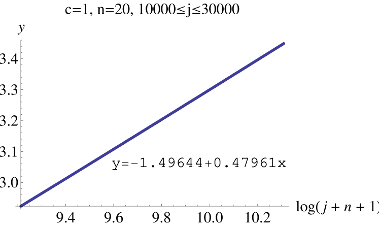
(a)

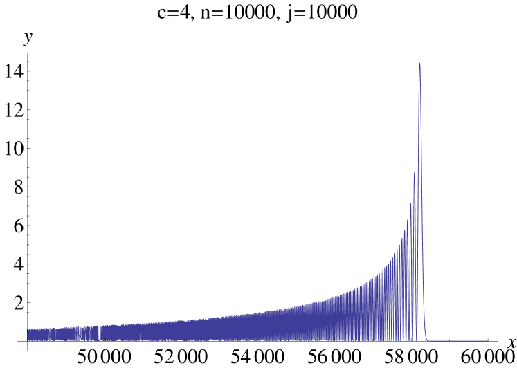
(b)

Figure 2. Numerical Calculations

In (A), to confirm the case $c=1$, $y=\log\left(\frac{n!}{(n+j)!}\max_{\lambda\geq 0}e^{-\lambda}\lambda^{1+j}\left|L^{j}_{0}\right|^{2}(\lambda)\right)$ and $x=\log(j+n+1)$, where $n=20$, the data almost lies on a line. For a larger range of $j$, the slope is close to $0.5$. In (B), $y=\frac{n!(1+n)^{1/6}}{(n+j)!(n+j+1)^{c-1/2}}e^{-\lambda}\lambda^{(c+j)}\left|L_{n}^{j}\right|^{2}(\lambda)$. For fixed $c$, when we vary $n$ and $j$, from our numerical observation, $y$ is uniformly bounded. If we increase $c$, the bound increases.

Now we are ready to establish the collapsing estimate Theorem 2.

Proof.

By the Parseval’s theorem on $L^{2}([0,\pi/b])$,

$$\left\||\nabla_{x}|^{c}\gamma(t,x,x)\right\|_{L^{2}_{[0,\pi/b]}L^{2}_{x}}^{2} =\left\||\nabla_{x}|^{c}\sum_{j,k\in\mathbb{N}}e^{-2b(j-k)it}\gamma_{jk}(x,x)\right\|_{L^{2}_{[0,\pi/b]}L^{2}_{x}}^{2}$$

(87) $$=\frac{\pi}{b}\sum_{m\in\mathbb{Z}}\left\||\nabla_{x}|^{c}\sum_{\begin{subarray}{c}j-k=m\\ j,k\in\mathbb{N}\end{subarray}}\gamma_{jk}(x,x)\right\|_{L^{2}_{x}}^{2}.$$

We will express (87) by the Fourier transform of $|\nabla_{x}|^{c}\gamma_{jk}(x,x)$. Using the expression (78),

$$\left(\widehat{|\nabla_{x}|^{c}\gamma_{jk}(x,x)}\right)(\xi) =\frac{1}{2\pi}\int_{\mathbb{R}^{4}}d\tilde{x}d\tilde{y}\,|\xi|^{c}\gamma_{jk}(\tilde{x},\tilde{y})\left(e^{-i\xi\tilde{x}}W(h_{j})(\xi)\right)*\left(e^{-i\xi\tilde{y}}W(h_{k})(\xi)\right)$$

$$\quad*\delta\left(\xi+\frac{b}{2}J(\tilde{x}-\tilde{y})\right),$$

where $W(h_{j})=W(h_{j},h_{j})$. To compute $\left(e^{-i\xi\tilde{x}}W(h_{j})(\xi)\right)*\left(e^{-i\xi\tilde{y}}W(h_{k})(\xi)\right)$, using tools from Appendix 7.3

$$\left(e^{-i\xi\tilde{x}}W(h_{j})(\xi)\right)*\left(e^{-i\xi\tilde{y}}W(h_{k})(\xi)\right)$$

$$=\int_{\mathbb{R}^{2}}d\tilde{\xi}\,e^{-i\left(\xi-\tilde{\xi}\right)\tilde{x}}W(h_{j})\left(\xi-\tilde{\xi}\right)e^{-i\tilde{\xi}\tilde{y}}W(h_{k})\left(\tilde{\xi}\right)$$

$$=\int_{\mathbb{R}^{2}}d\tilde{\xi}\,e^{-i\left(\xi-\tilde{\xi}\right)\tilde{x}}W(h_{j})\left(\tilde{\xi}-\xi\right)e^{-i\tilde{\xi}\tilde{y}}W(h_{k})\left(\tilde{\xi}\right)$$

$$=e^{-i\xi\tilde{x}/2}\int_{\mathbb{R}^{2}}d\tilde{\xi}\,W\left(\beta\left(\frac{\tilde{x}}{2}-\frac{J\xi}{b}\right)h_{j},\beta\left(-\frac{\tilde{x}}{2}-\frac{J\xi}{b}\right)h_{j}\right)(\tilde{\xi})\overline{W\left(\beta\left(\frac{\tilde{y}}{2}\right)h_{k},\beta\left(-\frac{\tilde{y}}{2}\right)h_{k}\right)}(\tilde{\xi})$$

$$=\frac{2\pi e^{-i\xi\tilde{x}/2}}{b}\left\langle\beta\left(\frac{\tilde{x}}{2}-\frac{J\xi}{b}\right)h_{j},\beta\left(\frac{\tilde{y}}{2}\right)h_{k}\right\rangle\left\langle\beta\left(-\frac{\tilde{y}}{2}\right)h_{k},\beta\left(-\frac{\tilde{x}}{2}-\frac{J\xi}{b}\right)h_{j}\right\rangle$$

$$=\frac{2\pi e^{-i\xi\tilde{x}/2}}{b}\left\langle\beta\left(-\frac{\tilde{y}}{2}\right)\beta\left(\frac{\tilde{x}}{2}-\frac{J\xi}{b}\right)h_{j},h_{k}\right\rangle\left\langle\beta\left(\frac{\tilde{x}}{2}+\frac{J\xi}{b}\right)\beta\left(-\frac{\tilde{y}}{2}\right)h_{k},h_{j}\right\rangle$$

$$=\frac{2\pi e^{-i\left(\tilde{x}+\tilde{y}\right)\xi}}{b}V\left(h_{j},h_{k}\right)\left(\frac{\tilde{x}-\tilde{y}}{2}-\frac{J\xi}{b}\right)V\left(h_{k},h_{j}\right)\left(\frac{\tilde{x}-\tilde{y}}{2}+\frac{J\xi}{b}\right).$$

Then

$$\left(\widehat{|\nabla_{x}|^{c}\gamma_{jk}(x,x)}\right)(\xi) =\frac{1}{b}\int_{\mathbb{R}^{4}}d\tilde{x}d\tilde{y}\,|\xi|^{c}\gamma_{jk}(\tilde{x},\tilde{y})\exp\left(-\frac{i}{2}\left[(\tilde{x}+\tilde{y})\xi+\frac{b}{2}\,\Omega(\tilde{x}+\tilde{y},\tilde{x}-\tilde{y})\right]\right)\times$$

$$\quad V(h_{j},h_{k})\left(\tilde{x}-\tilde{y}-\frac{J\xi}{b}\right)V(h_{k},h_{j})\left(\frac{J\xi}{b}\right).$$

Next estimate (87), using the Fourier transform on $\tilde{x}+\tilde{y}$ and the Minkowski inequality,

$$(\ref{collapsing,term,c}) \lesssim b^{-3}\sum_{m\in\mathbb{Z}}\left(\sum_{\begin{subarray}{c}j-k=m\\ j,k\in\mathbb{N}\end{subarray}}\left\|\int_{\mathbb{R}^{2}}d(\tilde{x}-\tilde{y})\,|\xi|^{c}\mathcal{F}_{\tilde{x}+\tilde{y}}\left(\gamma_{jk}\right)\left(\frac{1}{2}\left(\xi+\frac{bJ(\tilde{x}-\tilde{y})}{2}\right),\tilde{x}-\tilde{y}\right)\times\right.\right.$$

$$\quad\left.\left.V(h_{j},h_{k})\left(\tilde{x}-\tilde{y}-\frac{J\xi}{b}\right)V(h_{k},h_{j})\left(\frac{J\xi}{b}\right)\right\|_{L^{2}_{\xi}}\right)^{2}$$

$$\lesssim b^{-3}\sum_{m\in\mathbb{Z}}\left(\sum_{\begin{subarray}{c}j-k=m\\ j,k\in\mathbb{N}\end{subarray}}\left\|V(h_{j},h_{k})\right\|_{L^{2}_{\mathbb{R}^{2}}}\|\gamma_{jk}\|_{L^{2}_{\mathbb{R}^{4}}}\sup_{\xi\in\mathbb{R}^{2}}|\xi|^{c}\left|V(h_{k},h_{j})\right|\left(\frac{J\xi}{b}\right)\right)^{2}$$

$$\qquad(\hbox{Cauchy-Schwartz inequality})$$

$$\lesssim b^{-4}\sup_{m\in\mathbb{Z}}\left(\sum_{\begin{subarray}{c}j-k=m\\ j,k\in\mathbb{N}\end{subarray}}\frac{1}{\langle 2bj\rangle^{s}\langle 2bk\rangle^{s}}\sup_{\xi\in\mathbb{R}^{2}}|\xi|^{2c}\left|V(h_{j},h_{k})\right|^{2}\left(\frac{J\xi}{b}\right)\right)\sum_{j,k\in\mathbb{N}}\langle 2bj\rangle^{s}\langle 2bk\rangle^{s}\|\gamma_{jk}\|_{L^{2}_{\mathbb{R}^{4}}}^{2}.$$

$$\qquad\left(\hbox{since }\left\|V(h_{j},h_{k})\right\|_{L^{2}_{\mathbb{R}^{2}}}^{2}=\frac{2\pi}{b}\langle h_{k},h_{k}\rangle\langle h_{j},h_{j}\rangle=\frac{2\pi}{b}\right)$$

The estimate (43) reduces to show

$$b^{-4}\sup_{m\in\mathbb{N}}\left(\sum_{\begin{subarray}{c}j-k=m\\ j,k\in\mathbb{N}\end{subarray}}\frac{1}{\langle 2bj\rangle^{s}\langle 2bk\rangle^{s}}\sup_{\xi\in\mathbb{R}^{2}}|\xi|^{2c}\left|V(h_{j},h_{k})\right|^{2}\left(\frac{J\xi}{b}\right)\right)<\infty.$$

Taking $c=0$, by Lemma 4, for any $m\in\mathbb{N}$,

$$\sum_{\begin{subarray}{c}j-k=m\\ j,k\in\mathbb{N}\end{subarray}}\frac{1}{\langle 2bj\rangle^{s}\langle 2bk\rangle^{s}}\left\|V(h_{j},h_{k})\left(\frac{J\xi}{b}\right)\right\|_{L^{\infty}}^{2}\leq\sum_{\begin{subarray}{c}j-k=m\\ k\in\mathbb{N}\end{subarray}}\frac{1}{\langle 2bj\rangle^{s}\langle 2bk\rangle^{s}}\leq\sum_{k\in\mathbb{N}}\frac{1}{\langle 2bk\rangle^{2s}},$$

which is finite if $s>1/2$. Taking $1\leq c\leq 2$, by Lemma 5,

$$\sum_{\begin{subarray}{c}j-k=m\\ j,k\in\mathbb{N}\end{subarray}}\frac{1}{\langle 2bj\rangle^{s}\langle 2bk\rangle^{s}}\left\||\xi|^{c}V(h_{j},h_{k})\left(\frac{J\xi}{b}\right)\right\|_{L^{\infty}}^{2} \lesssim\sum_{\begin{subarray}{c}j-k=m\\ k\in\mathbb{N}\end{subarray}}\frac{b^{c}\langle k\rangle^{(2-c)/6}\langle j\rangle^{(3c-2)/2}}{\langle 2bj\rangle^{s}\langle 2bk\rangle^{s}}$$

$$\lesssim\frac{1}{b^{2s-c}}\sum_{k\in\mathbb{N}}\frac{1}{\langle k\rangle^{2s-4c/3+2/3}},$$

which is finite if $2s-4c/3+2/3>1$. Setting $s=1$, we get $1\leq c<5/4$.

Combining the low frequency case $c=0$ and the high frequency case $1\leq c<5/4$ yields the estimate (43). ∎

5. Well-Posedness of the System

Before showing the local well-posedness result Theorem 1, we discuss Equation (22) in a case other than Equation (27) to demonstrate that $[\rho_{Q}*v,_{\phi}]$ in Equation $(\ref{equation,pertubation})$ is a trouble term. Equation (22) is well-posed in several spaces. The possible low regularity for the initial data when we can obtain a local well-posedness result is

(88) $$\left\|H_{hx}^{1/8+\epsilon}H_{hy}^{1/8+\epsilon}\gamma_{0}(x,y)\right\|_{L^{2}_{x}L^{2}_{y}}<\infty,\quad x,y\in\mathbb{R}^{2},\quad\hbox{for arbitrary}\ \epsilon>0,$$

where the norm is

$$\left\|H_{h}^{s/2}f\right\|_{L^{2}}=\left\||\nabla|^{s}f\right\|_{L^{2}}+\left\||x|^{s}f\right\|_{L^{2}},\quad s\geq 0,\ f\in L^{2}(\mathbb{R}^{2}).$$

For the initial data (88), we acquire the following result.

Theorem 5.

Consider Equation (22) and suppose the initial condition $\gamma_{0}$ satisfies (88). Then Equation (22) has a mild solution for sufficiently short time $T$ in the Banach $\mathbf{N}_{HT}$, where the norm is defined as

(89) $$\|\gamma\|_{\mathbf{N}_{HT}}:=\left\|H_{hx}^{1/8+\epsilon}H_{hy}^{1/8+\epsilon}\gamma(t,x,y)\right\|_{L^{\infty}_{I_{T}}L^{2}_{x}L^{2}_{y}}+\left\||\nabla|^{1/2+2\epsilon}\rho_{\gamma}(t,x)\right\|_{L^{2}_{I_{T}}L^{2}_{x}},$$

where $I_{T}=[0,T]$ and the $\epsilon$ is the same in (88).

Remark 11.

Notice that the initial condition only requires that $\gamma_{0}$ is a Hilbert-Schmidt operator. It is not necessarily of trace class.

In order to use the technique in [GM17, Section 5, Section 6] to prove Theorem 5, we need another version of the collapsing estimate

Proposition 2.

Suppose $\gamma(t,x,y)=e^{-i(H_{x}-\bar{H}_{y})}\gamma_{0}(x,y)$ is the solution to the linear equation

(92) $$\left\{\begin{array}[]{l}i\,\partial_{t}\gamma=\left[H,\gamma\right],\\ \gamma(0,x,y)=\gamma_{0}(x,y)\in L^{2}_{x}L^{2}_{y},\end{array}\right.\quad x,y\in\mathbb{R}^{2},$$

the collapsing term $\rho_{\gamma}(t,x)=\gamma(t,x,x)$ satisfies

(93) $$\left\|\langle\tan bt\rangle^{-1/2-\epsilon}|\nabla_{x}|^{1/2+2\epsilon}\rho_{\gamma}(t,x)\right\|_{L^{2}_{[-\pi/2b,\pi/2b]}L^{2}_{x}}\lesssim_{\epsilon}\left\|\langle\nabla_{x}\rangle^{1/4+\epsilon}\langle\nabla_{y}\rangle^{1/4+\epsilon}\gamma_{0}(x,y)\right\|_{L^{2}_{x}L^{2}_{y}},$$

where $\epsilon$ is any arbitrary small positive number.

Proof.

The operator $H$ is decomposed as (66) and $[H_{h},H_{r}]=0$. Since the rotation generated by the vector field $-iH_{r}$ satisfies

$$\left||\nabla|^{s}e^{-iH_{r}t}f\right|(x)=\left||\nabla|^{s}f\right|\left(e^{-iH_{r}t}x\right),\quad x\in\mathbb{R}^{2}$$

and $e^{-i(H_{rx}-\bar{H}_{ry})t}\gamma_{0}(x,y)=e^{-i(H_{rx}+H_{ry})t}\gamma_{0}(x,y)$,

$$\left\|\langle\tan bt\rangle^{-1/2-\epsilon}|\nabla_{x}|^{1/2+2\epsilon}\rho_{\gamma}(t,x)\right\|_{L^{2}_{[-\pi/2b,\pi/2b]}L^{2}_{x}}$$

$$= \left\|\langle\tan bt\rangle^{-1/2-\epsilon}|\nabla_{x}|^{1/2+2\epsilon}\left(e^{-i\left(H_{rx}-\bar{H}_{ry}\right)t}e^{-i(H_{hx}-\bar{H}_{hy})t}\gamma_{0}\right)(x,x)\right\|_{L^{2}_{[-\pi/2b,\pi/2b]}L^{2}_{x}}$$

$$= \left\|\langle\tan bt\rangle^{-1/2-\epsilon}|\nabla_{x}|^{1/2+2\epsilon}\left(e^{-i(H_{hx}-\bar{H}_{hy})t}\gamma_{0}\right)(x,x)\right\|_{L^{2}_{[-\pi/2b,\pi/2b]}L^{2}_{x}}.$$

Then the estimate (93) reduces to

$$\left\|\langle\tan bt\rangle^{-1/2-\epsilon}|\nabla_{x}|^{1/2+2\epsilon}\left(e^{-i(H_{hx}-\bar{H}_{hy})t}\gamma_{0}\right)(x,x)\right\|_{L^{2}_{[-\pi/2b,\pi/2b]}L^{2}_{x}}\lesssim_{\epsilon}\left\|\langle\nabla_{x}\rangle^{1/4+\epsilon}\langle\nabla_{y}\rangle^{1/4+\epsilon}\gamma_{0}(x,y)\right\|_{L^{2}_{x}L^{2}_{y}},$$

where the collapsing term corresponds to the equation $i\,\partial_{t}\gamma=\left[H_{h},\gamma\right]$. By the Lens transform [Tao09]

(94) $$\L(u)(t,x):=\frac{1}{\cos bt}u\left(\frac{\tan bt}{b},\frac{x}{\cos bt}\right)e^{-\left(ib|x|^{2}\tan bt\right)/4},\quad t\in\mathbb{R},\ x\in\mathbb{R}^{2},$$

which maps the solution $u(t,x)$ of $i\,\partial_{t}u=-\Delta u$ to the solution of $i\,\partial_{t}\L(u)=H_{h}\L(u)$, we obtain the identity

$$\left\|\langle\tan bt\rangle^{-1/2-\epsilon}|\nabla_{x}|^{1/2+2\epsilon}\left(e^{-i(H_{hx}-\bar{H}_{hy})t}\gamma_{0}\right)(x,x)\right\|_{L^{2}_{[-\pi/2b,\pi/2b]}L^{2}_{x}}$$

$$= \left\||\nabla_{x}|^{1/2+2\epsilon}\left(e^{i(\Delta_{x}-\Delta_{y})t}\gamma_{0}\right)(x,x)\right\|_{L^{2}_{t}L^{2}_{x}}.$$

Finally, the estimate (93) reduces to the Laplacian case

$$\left\||\nabla_{x}|^{1/2+2\epsilon}\left(e^{i(\Delta_{x}-\Delta_{y})t}\gamma_{0}\right)(x,x)\right\|_{L^{2}_{t}L^{2}_{x}}\lesssim_{\epsilon}\left\|\langle\nabla_{x}\rangle^{1/4+\epsilon}\langle\nabla_{y}\rangle^{1/4+\epsilon}\gamma_{0}(x,y)\right\|_{L^{2}_{x}L^{2}_{y}},$$

which is proved in [GM17, CHP17]. ∎

Since the Hermite operator $H_{h}$ dominates $-\Delta+1$ in the sense $\left\|\langle-\Delta\rangle^{s/2}f\right\|_{L^{2}}\lesssim\left\|H_{h}^{s/2}f\right\|_{L^{2}}$ for $s\geq 0$, as a corollary of Proposition 2

(95) $$\left\|\langle\tan bt\rangle^{-1/2-\epsilon}|\nabla_{x}|^{1/2+2\epsilon}\rho_{\gamma}(t,x)\right\|_{L^{2}_{[-\pi/2b,\pi/2b]}L^{2}_{x}}\lesssim_{\epsilon}\left\|H_{hx}^{1/8+\epsilon}H_{hy}^{1/8+\epsilon}\gamma_{0}(x,y)\right\|_{L^{2}_{x}L^{2}_{y}}.$$

using this estimate (95) and the scheme in [GM17], Theorem 5 follows.

When it comes to Equation (27), if we expect to establish a local well-posedness result when

$$\left\|H_{hx}^{s/2}H_{hy}^{s/2}Q_{0}(x,y)\right\|_{L^{2}_{x}L^{2}_{y}}<\infty,$$

we need to deal with terms, for example $\left\|\left|\nabla_{x}\right|^{s}\left(\rho_{Q}*v\right)H_{hy}^{s/2}\bar{\Pi}_{\phi}(x,y)\right\|_{L^{2}_{x}L^{2}_{y}}$. However $H_{hy}^{s/2}\bar{\Pi}_{\phi}$ is not translation invariant. After integrating over $y$, we are faced with $\left\||x|^{s}\left|\nabla_{x}\right|^{s}\left(\rho_{Q}*v\right)\right\|_{L^{2}}$. For the linear equation $i\,\partial_{t}Q=[H+\rho_{Q}*v,Q]$ and $Q(t=0)=Q_{0}$, $\left\||x|^{s}\left|\nabla_{x}\right|^{s}\left(\rho_{Q}*v\right)\right\|_{L^{2}_{I_{T}}L^{2}}$ is controlled by $\left\|H_{hx}^{s/2}H_{hy}^{s/2}Q_{0}(x,y)\right\|_{tr}$. But it may not be controlled by $\left\|H_{hx}^{s/2}H_{hy}^{s/2}Q_{0}(x,y)\right\|_{L^{2}_{x}L^{2}_{y}}$. Therefore we can not close the argument to obtain a local well-posedness result of Equation (27). That is why we stick to the structure of Equation (27) and use norms arising from $H$, i.e. Definition 1. The operator $H$ is more compatible with the stationary solution $\bar{\Pi}_{\phi}$ than $H_{h}$. Hence we can deal with $\langle H_{x}\rangle^{1/2}\langle\bar{H}_{y}\rangle^{1/2}[\rho_{Q}*v,\bar{\Pi}_{\phi}]$.

Next we prove Theorem 1 the local wellposedness result of Equation (27).

Proof.

By Duhamel’s formulation, we define the solution map $\Phi$ and the solution ball $sol_{T}$ for the contraction mapping principle,

(96) $$\Phi(Q)(t,x,y):=e^{-i(H_{x}-\bar{H}_{y})t}Q_{0}-i\int_{0}^{t}e^{-i(H_{x}-\bar{H}_{y})(t-\tau)}[v*\rho_{Q},Q+\bar{\Pi}_{\phi}](\tau)\,d\tau,$$

(97) $$sol_{T}:=\left\{Q(t,x,y)\left|\|Q(t,x,y)\|_{\mathbf{N}_{T}}\leq C\left\|\langle H_{x}\rangle^{1/2}\langle\bar{H}_{y}\rangle^{1/2}Q_{0}(x,y)\right\|_{L_{x}^{2}L_{y}^{2}}\right.\right\},$$

where parameters $T$ and $C>1$ are to be determined later.

1. Show $\Phi$ maps $sol_{T}$ to itself.

Suppose $Q\in sol_{T}$. By Theorem 2 and Proposition 1,

$$\|e^{-i(H_{x}-\bar{H}_{y})t}Q_{0}\|_{\mathbf{N}_{T}}\lesssim_{T}\left\|\langle H_{x}\rangle^{1/2}\langle\bar{H}_{y}\rangle^{1/2}Q_{0}\right\|_{L_{x}^{2}L_{y}^{2}}.$$

Choosing $T=\pi/4b$, then $C$ is the constant such that

$$\|e^{-i(H_{x}-\bar{H}_{y})t}Q_{0}\|_{\mathbf{N}_{T}}\leq C\left\|\langle H_{x}\rangle^{1/2}\langle\bar{H}_{y}\rangle^{1/2}Q_{0}\right\|_{L_{x}^{2}L_{y}^{2}}/2.$$

For the nonlinear part, claim the estimate

(98) $$\left\|\int_{0}^{t}e^{-i(H_{x}-\bar{H}_{y})(t-\tau)}[v*\rho_{Q},Q+\bar{\Pi}_{\phi}](\tau)\,d\tau\right\|_{\mathbf{N}_{T}}\lesssim\left\|\langle H_{x}\rangle^{1/2}\langle\bar{H}_{y}\rangle^{1/2}[v*\rho_{Q},Q+\bar{\Pi}_{\phi}]\right\|_{L^{1}_{I_{T}}L^{2}_{x}L^{2}_{y}}.$$

The proof of (98) is twofold. On one hand, to control the Strichartz norm,

$$\left\|\int_{0}^{t}e^{-i(H_{x}-\bar{H}_{y})(t-\tau)}\underbrace{\langle H_{x}\rangle^{1/2}\langle\bar{H}_{y}\rangle^{1/2}[v*\rho_{Q},Q+\bar{\Pi}_{\phi}](\tau)}_{F_{1}(\tau,x,y)}\,d\tau\right\|_{L^{q}_{I_{T}}L^{r}_{x}L^{2}_{y}},$$

suppose $G(t,x,y)$ is in the dual Strichartz space $L_{I_{T}}^{q^{\prime}}L_{x}^{r^{\prime}}L^{2}_{y}$, where

$$\frac{1}{q}+\frac{1}{q^{\prime}}=1,\quad\frac{1}{r}+\frac{1}{r^{\prime}}=1.$$

Using the dual characterization of $L^{p}$ spaces

$$\int_{I_{T}}\int_{\mathbb{R}^{2}\times\mathbb{R}^{2}}dtdxdy\,\bar{G}(t,x,y)\int_{0}^{t}e^{-i(H_{x}-\bar{H}_{y})(t-\tau)}F_{1}(\tau,x,y)d\tau$$

$$= \int_{I_{T}}\int_{\mathbb{R}^{2}\times\mathbb{R}^{2}}d\tau dxdy\,F_{1}(\tau,x,y)\int_{\tau}^{T}\overline{e^{-i(H_{x}-\bar{H}_{y})(\tau-t)}G}(t,x,y)\,dt$$

$$\leq \int_{I_{T}}d\tau\,\left\|F_{1}(\tau,x,y)\right\|_{L^{2}_{x}L^{2}_{y}}\left\|\int_{\tau}^{T}\overline{e^{-i(H_{x}-\bar{H}_{y})(\tau-t)}G}(t,x,y)\,dt\right\|_{L^{\infty}_{I_{T}}L^{2}_{x}L^{2}_{y}}$$

$$\lesssim \int_{I_{T}}d\tau\,\left\|F_{1}(\tau,x,y)\right\|_{L^{2}_{x}L^{2}_{y}}\left\|G(t,x,y)\right\|_{L^{q^{\prime}}_{I_{T}}L^{r^{\prime}}_{x}L^{2}_{y}},$$

$$\quad(\text{by Proposition \ref{Strichartz,homogeneous} the dual Strichartz estimate (\ref{dual,strichartz})})$$

we obtain,

$$\left\|\int_{0}^{t}e^{-i\left(H_{x}-\bar{H}_{y}\right)(t-\tau)}F_{1}(\tau,x,y)\,d\tau\right\|_{L^{q}_{I_{T}}L^{r}_{x}L^{2}_{y}}\lesssim\left\|F_{1}(t,x,y)\right\|_{L^{1}_{I_{T}}L^{2}_{x}L^{2}_{y}}.$$

The argument for the norm $L^{q}_{I_{T}}L^{r}_{y}L^{2}_{x}$ is the same. On the other hand, to control the collapsing term

$$\left\|\langle\nabla_{x}\rangle^{9/8}\left(\int_{0}^{t}e^{-i(H_{x}-\bar{H}_{y})(t-\tau)}\underbrace{[v*\rho_{Q},Q+\bar{\Pi}_{\phi}](\tau)}_{F_{2}(\tau,x,y)}\,d\tau\right)(t,x,x)\right\|_{L^{2}_{I_{T}}L^{2}_{x}},$$

applying Theorem 2 and the Minkowski inequality,

$$\left\|\langle\nabla_{x}\rangle^{9/8}\left(\int_{0}^{t}e^{-i(H_{x}-\bar{H}_{y})(t-\tau)}F_{2}(\tau,x,y)\,d\tau\right)(t,x,x)\right\|_{L^{2}_{I_{T}}L^{2}_{x}}$$

$$\leq \left\|\int_{0}^{T}\left\|\langle\nabla_{x}\rangle^{9/8}\left(e^{-i(H_{x}-\bar{H}_{y})(t-\tau)}F_{2}(\tau,x,y)\right)(t,x,x)\right\|_{L^{2}_{x}}d\tau\right\|_{L^{2}_{I_{T}}}$$

$$\leq \int_{0}^{T}d\tau\left\|\langle\nabla_{x}\rangle^{9/8}\left(e^{-i(H_{x}-\bar{H}_{y})(t-\tau)}F_{2}(\tau,x,y)\right)(t,x,x)\right\|_{L^{2}_{I_{T}}L^{2}_{x}}$$

$$\lesssim \int_{0}^{T}d\tau\left\|\langle H_{x}\rangle^{1/2}\langle\bar{H}_{y}\rangle^{1/2}F_{2}(\tau,x,y)\right\|_{L^{2}_{x}L^{2}_{y}}\quad(\text{by Theorem \ref{pauli,collapsing,estimate}}).$$

According to the estimate (98), the problem is reduced to estimate quantities

$$\left\|\langle H_{x}\rangle^{1/2}\langle\bar{H}_{y}\rangle^{1/2}[v*\rho_{Q},Q]\right\|_{L^{1}_{I_{T}}L^{2}_{x}L^{2}_{y}},\quad\left\|\langle H_{x}\rangle^{1/2}\langle\bar{H}_{y}\rangle^{1/2}[v*\rho_{Q},\bar{\Pi}_{\phi}]\right\|_{L^{1}_{I_{T}}L^{2}_{x}L^{2}_{y}}.$$

Since the commutation relation does not play a role of our analysis, we give proofs for one of the two terms in the commutation relation. The other one is dealt similarly.

Considering $\left\|\langle H_{x}\rangle^{1/2}\langle\bar{H}_{y}\rangle^{1/2}\left(\left(v*\rho_{Q}\right)(t,x)Q(t,x,y)\right)\right\|_{L^{1}_{I_{T}}L^{2}_{x}L^{2}_{y}}$, based on the observation (71), we estimate it by

$$\lesssim\left\|D_{x}\langle\bar{H}_{y}\rangle^{1/2}\left(v*\rho_{Q}\right)(t,x)Q(t,x,y)\right\|_{L^{1}_{I_{T}}L^{2}_{x}L^{2}_{y}}+\left\|\langle\bar{H}_{y}\rangle^{1/2}\left(v*\rho_{Q}\right)(t,x)Q(t,x,y)\right\|_{L^{1}_{I_{T}}L^{2}_{x}L^{2}_{y}}$$

$$\lesssim\left\|2\partial_{z_{x}}\left(v*\rho_{Q}\right)(t,x)\,\langle\bar{H}_{y}\rangle^{1/2}Q(t,x,y)\right\|_{L^{1}_{I_{T}}L^{2}_{x}L^{2}_{y}}+\left\|\left(v*\rho_{Q}\right)(t,x)\langle H_{x}\rangle^{1/2}\langle\bar{H}_{y}\rangle^{1/2}Q(t,x,y)\right\|_{L^{1}_{I_{T}}L_{x}^{2}L_{y}^{2}}$$

$$\lesssim T^{1/2}\left\||\nabla_{x}|(v*\rho_{Q})(t,x)\right\|_{L^{2}_{I_{T}}L^{\frac{16}{7}}_{x}}\left\|\langle\bar{H}_{y}\rangle^{1/2}Q(t,x,y)\right\|_{L^{\infty}_{I_{T}}L^{16}_{x}L^{2}_{y}}$$

$$\quad+T^{1/4}\left\|\left(v*\rho_{Q}\right)(t,x)\right\|_{L^{2}_{I_{T}}L^{4}_{x}}\left\|\langle H_{x}\rangle^{1/2}\langle\bar{H}_{y}\rangle^{1/2}Q(t,x,y)\right\|_{L^{4}_{I_{T}}L_{x}^{4}L_{y}^{2}}\quad(\text{by H\"{o}lder inequality})$$

$$\lesssim T^{1/2}\left\||\nabla_{x}|^{9/8}\rho_{Q}(t,x)\right\|_{L^{2}_{I_{T}}L^{2}_{x}}\|\langle H_{x}\rangle^{1/2}\langle\bar{H}_{y}\rangle^{1/2}Q(t,x,y)\|_{L^{\infty}_{I_{T}}L^{2}_{x}L^{2}_{y}}$$

$$\quad+T^{1/4}\left\||\nabla_{x}|^{1/2}\rho_{Q}(t,x)\right\|_{L^{2}_{I_{T}}L^{2}_{x}}\left\|\langle H_{x}\rangle^{1/2}\langle\bar{H}_{y}\rangle^{1/2}Q(t,x,y)\right\|_{L^{4}_{I_{T}}L^{4}_{x}L^{2}_{y}}$$

$$\qquad(\text{by Sobolev inequality, Lemma \ref{covariant,n-endpoint,sobolev} and Young's convolution inequality})$$

$$\lesssim\max\{T^{1/2},T^{1/4}\}\left\|Q(t)\right\|_{\mathbf{N}_{T}}^{2}$$

$$\lesssim\max\{T^{1/2},T^{1/4}\}\left\|\langle H_{x}\rangle^{1/2}\langle\bar{H}_{y}\rangle^{1/2}Q_{0}(x,y)\right\|_{L_{x}^{2}L_{y}^{2}}^{2}.$$

Then for $\left\|\langle H_{x}\rangle^{1/2}\langle\bar{H}_{y}\rangle^{1/2}[v*\rho_{Q},\bar{\Pi}_{\phi}]\right\|_{L^{1}_{I_{T}}L^{2}_{x}L^{2}_{y}}$, because of direct computation

$$\bar{D}_{y}\bar{\Pi}_{\phi}(x,y) =\left(2\partial_{z}\phi(x-y)+\frac{b}{2}(\bar{z}_{x}-\bar{z}_{y})\phi(x-y)\right)e^{-ib\Omega(x,y)/2},$$

$$D_{x}\bar{\Pi}_{\phi}(x,y) =\left(-2\partial_{\bar{z}}\phi(x-y)-\frac{b}{2}(z_{x}-z_{y})\phi(x-y)\right)e^{-ib\Omega(x,y)/2},$$

$$D_{x}\bar{D}_{y}\bar{\Pi}_{\phi}(x,y) =\left(-4\partial_{\bar{z}}\partial_{z}\phi(x-y)-b(z_{x}-z_{y})\partial_{z}\phi(x-y)\right.$$

$$\quad\left.-b(\bar{z}_{x}-\bar{z}_{y})\partial_{\bar{z}}\phi(x-y)-\frac{b^{2}}{4}|x-y|^{2}\phi(x-y)\right)e^{-ib\Omega(x,y)/2},$$

integrating over $x$ or $y$, we obtain

$$\left\|\bar{D}_{y}\bar{\Pi}_{\phi}(x,y)\right\|_{L^{2}_{x(y)}}=\left\|\bar{D}\phi\right\|_{L^{2}}\lesssim\left\|\langle\bar{H}\rangle^{1/2}\phi\right\|_{L^{2}}$$

$$\left\|D_{x}\bar{\Pi}_{\phi}(x,y)\right\|_{L^{2}_{x(y)}}=\left\|D\phi\right\|_{L^{2}}\lesssim\left\|\langle H\rangle^{1/2}\phi\right\|_{L^{2}},$$

$$\left\|D_{x}\bar{D}_{y}\bar{\Pi}_{\phi}(x,y)\right\|_{L^{2}_{x(y)}}=\left\|D\bar{D}\phi\right\|_{L^{2}}\lesssim\left\|\langle H\rangle^{1/2}\langle\bar{H}\rangle^{1/2}\phi\right\|_{L^{2}}.$$

Combining the above estimates,

$$\left\|\langle H_{x}\rangle^{1/2}\langle\bar{H}_{y}\rangle^{1/2}[v*\rho_{Q},\bar{\Pi}_{\phi}]\right\|_{L^{1}_{I_{T}}L^{2}_{x}L^{2}_{y}} \lesssim\left\|\langle\nabla_{x}\rangle\rho_{Q}(t,x)\right\|_{L^{1}_{I_{T}}L^{2}_{x}}\left\|\langle H\rangle^{1/2}\langle\bar{H}\rangle^{1/2}\phi\right\|_{L^{2}}$$

$$\lesssim T^{1/2}\left\|\langle H_{x}\rangle^{1/2}\langle\bar{H}_{y}\rangle^{1/2}Q_{0}(x,y)\right\|_{L_{x}^{2}L_{y}^{2}}\left\|\langle H\rangle^{1/2}\langle\bar{H}\rangle^{1/2}\phi\right\|_{L^{2}}$$

If necessary, shrink the interval $I_{T}$ such that

$$\left\|\int_{0}^{t}e^{-i(H_{x}-\bar{H}_{y})(t-\tau)}[v*\rho_{Q},Q+\bar{\Pi}_{\phi}](\tau)\,d\tau\right\|_{\mathbf{N}_{T}}\leq\frac{C}{2}\left\|\langle H_{x}\rangle^{1/2}\langle\bar{H}_{y}\rangle^{1/2}Q_{0}(x,y)\right\|_{L_{x}^{2}L_{y}^{2}}.$$

Thus $\Phi$ maps $sol_{T}$ to itself.

2. Show $\Phi$ is a contraction map.

For any $Q_{1},\,Q_{2}\in sol_{T}$, similarly as step 1,

$$\left\|\Phi(Q_{1})-\Phi(Q_{2})\right\|_{\mathbf{N}_{T}} \leq\left\|\int_{0}^{t}d\tau\,e^{-i(H_{x}-\bar{H}_{y})(t-\tau)}[v*\rho_{Q_{1}}-v*\rho_{Q_{2}},\bar{\Pi}_{\phi}]\right\|_{\mathbf{N}_{T}}$$

$$\quad+\left\|\int_{0}^{t}d\tau\,e^{-i(H_{x}-\bar{H}_{y})(t-\tau)}[v*\rho_{Q_{1}}-v*\rho_{Q_{2}},Q_{1}]\right\|_{\mathbf{N}_{T}}$$

$$\quad+\left\|\int_{0}^{t}d\tau\,e^{-i(H_{x}-\bar{H}_{y})(t-\tau)}[v*\rho_{Q_{2}},Q_{1}-Q_{2}]\right\|_{\mathbf{N}_{T}}$$

$$\lesssim T^{1/2}\|\langle\nabla_{x}\rangle(\rho_{Q_{1}}-\rho_{Q_{2}})\|_{L^{2}_{I_{T}}L^{2}_{x}}\left\|\langle H\rangle^{1/2}\langle\bar{H}\rangle^{1/2}\phi\right\|_{L^{2}}$$

$$\quad+\max\{T^{1/2},T^{1/4}\}\|Q_{1}-Q_{2}\|_{\mathbf{N}_{T}}\left(\|Q_{1}\|_{\mathbf{N}_{T}}+\|Q_{2}\|_{\mathbf{N}_{T}}\right)$$

$$\lesssim\max\{T^{1/2},T^{1/4}\}\|Q_{1}-Q_{2}\|_{\mathbf{N}_{T}}\left\|\langle H_{x}\rangle^{1/2}\langle\bar{H}_{y}\rangle^{1/2}Q_{0}(x,y)\right\|_{L_{x}^{2}L_{y}^{2}}.$$

If needed, choose a smaller $T$ such that $\left\|\Phi(Q_{1})-\Phi(Q_{2})\right\|_{\mathbf{N}_{T}}\leq\|Q_{1}-Q_{2}\|_{\mathbf{N}_{T}}/2$.

Then by the contraction mapping principle, $\Phi$ has a fixed point in $sol_{T}$, i.e. Equation (27) is locally well-posed. ∎

Remark 12.

There are two families of stationary solutions $\Pi_{\phi}$ and $\bar{\Pi}_{\phi}$ (see Section 7.2). The reason for only $\bar{\Pi}_{\phi}$ is used in our pertubation problem is twofold. On one hand, $\bar{\Pi}_{\phi}$ recovers the Fermi-Dirac distribution. On the other hand, suppose we use the stationary solution $\Pi_{\phi}$ instead of $\bar{\Pi}_{\phi}$. By the product rule of the covariant derivative $D$, $D(fg)=(Df)g-2f\partial_{\bar{z}}g$,

$$D_{x}\bar{D}_{y}\left(\rho_{u}*v(x)\Pi_{\phi}(x,y)\right)=D_{x}\left(\rho_{u}*v\right)(x)\bar{D}_{y}\Pi_{\phi}(x,y)+\left(\rho_{u}*v\right)(x)\left(-2\partial_{\bar{z}_{x}}\right)\bar{D}_{y}\Pi_{\phi}(x,y)$$

(99) or $$D_{x}\bar{D}_{y}\left(\rho_{u}*v(x)\Pi_{\phi}(x,y)\right)=(-2\partial_{\bar{z}_{x}})\left(\rho_{u}*v\right)(x)\bar{D}_{y}\Pi_{\phi}(x,y)+\left(\rho_{u}*v\right)(x)D_{x}\bar{D}_{y}\Pi_{\phi}(x,y).$$

Since we do not have an estimate for $D_{x}\rho_{u}(t,x)$, we use the form (99) to continue our argument. A direct computation shows

$$\bar{D}_{y}\Pi_{\phi}(x,y)=\left(2\partial_{z}\phi(x-y)-\frac{b}{2}(\bar{z}_{x}+\bar{z}_{y})\phi(x-y)\right)e^{ib\Omega(x,y)/2}.$$

$\left|\bar{D}_{y}\Pi_{\phi}(x,y)\right|$ is not translation invariant. Therefore in order to estimate

$$\left\|-2\partial_{\bar{z}_{x}}(\rho_{u}*v)(t,x)\bar{D}_{y}\Pi_{\phi}(x,y)\right\|_{L^{2}_{x}L^{2}_{y}},$$

we need to control $\left\|x|\nabla_{x}|\rho_{u}(t,x)\right\|_{L^{2}_{x}}$, which is not possible by using $\mathbf{N}_{T}$.

6. Conclusion

In this paper, we obtained a local well-posed result of Equation (27) and a new collapsing estimate Theorem 2. However the estimate is not sharp since we do not have an optimal control of associated Laguerre polynomials (see Remark 10).

The ultimate goal of Theorem 1 is to acquire a low regularity result, for example a local well-posedness result for the initial data

$$\left\|\langle H_{x}\rangle^{s/2}\langle\bar{H}_{y}\rangle^{s/2}Q_{0}(x,y)\right\|_{L^{2}_{x}L^{2}_{y}}<\infty,\quad s<1,$$

According to Remark 10 and the proof of Theorem 2, we have a little gain of derivatives for the collapsing term when $s>1/3$. We conjecture that the best case might be $s=1/3+\epsilon$. However it requires a fractional Leibniz rule for $\langle H\rangle^{s/2}(fg)$, which currently is beyond our ability.

Another direction is to establish a global well-posedness result when

$$\left\|\langle H_{x}\rangle^{1/2}\langle\bar{H}_{y}\rangle^{1/2}Q_{0}(x,y)\right\|_{Tr}<\infty.$$

A formal computation shows that the total energy of Equation (27) is conserved

(100) $$\mathcal{E}(Q)=Tr\left(H^{1/2}QH^{1/2}\right)+\frac{1}{2}\int_{\mathbb{R}^{2}}\left(v*\rho_{Q}\right)(x)\rho_{Q}(x)\,dx,$$

which can be used for the global well-posedness result. However we lack of tools to estimate $\left\|\rho_{Q}\bar{\Pi}_{\phi}\right\|_{Tr}$ by the initial data.

7. Appendix

7.1. Heisenberg Group

[Fol89, Chapter 1]Let us review the Heisenberg group $H_{1}$ with the group law

$$(p_{1},q_{1},t_{1})\cdot(p_{2},q_{2},t_{2})=\left(p_{1}+p_{2},q_{1}+q_{2},t_{1}+t_{2}+b\frac{\Omega\left((p_{1},q_{1}),(p_{2},q_{2})\right)}{2}\right),$$

where $p_{i},q_{i}\in\mathbb{R}$, $t_{i}\in\mathbb{R}$, and impose a complex structure on $\mathbb{R}^{2}$, $z=p+q\,i$.

Identify the tangent space $TH_{1}$ with $\mathbb{R}^{3}\times\mathbb{R}^{3}$ and its basis by $\left\{\partial_{p},\partial_{q},\partial_{t}\right\}$. Then the differential of the left multiplication $L_{g}$, where $g=(p_{g},q_{g},t_{g})$, is

$$DL_{g}\left(\partial_{p},\partial_{q},\partial_{t}\right) =\left(\partial_{p},\partial_{q},\partial_{t}\right)\begin{pmatrix}1&0&0\\ 0&1&0\\ -bq_{g}/2&bp_{g}/2&1\end{pmatrix}.$$

The Lie algebra $\mathfrak{h}_{1}$ consisting of left invariant vector fields is

$$\mathfrak{h}_{1} =\mathbb{R}\hbox{-span}\left\{\partial_{p}-b\frac{q}{2}\partial_{t},\ \partial_{q}+b\frac{p}{2}\partial_{t},\ \partial_{t}\right\},$$

and the corresponding complexified space is

$$\mathfrak{h}_{1}^{\mathbb{C}} =\mathbb{C}\hbox{-span}\left\{2\partial_{\bar{z}}+i\frac{bz}{2}\partial_{t},\ 2\partial_{z}-i\frac{b\bar{z}}{2}\partial_{t},\ \partial_{t}\right\}.$$

We will think of $D$ and $D^{*}$ as vector fields of $\mathfrak{h}_{1}^{\mathbb{C}}$ in the following way. Denote

$$D_{H_{1}}=-2\partial_{\bar{z}}-i\frac{bz}{2}\partial_{t},\quad D^{*}_{H_{1}}=2\partial_{z}-i\frac{b\bar{z}}{2}\partial_{t}.$$

Suppose $\tilde{f}\in\mathcal{S}(H_{1})$ and apply the inverse Fourier transform on $t$ variable,

$$\check{D}_{H_{1}}\check{\tilde{f}}=\frac{1}{\sqrt{2\pi}}\int_{\mathbb{R}}\left(-2\partial_{\bar{z}}-\frac{bz\tau}{2}\right)\tilde{f}(q,p,t)e^{it\tau}\,dt.$$

On the piece $\tau=1$, $D_{H_{1}}$ and $D^{*}_{H_{1}}$ correspond to $D$ and $D^{*}$ respectively.

To make this correspondence rigorous, consider a quotient group $H_{1}^{red}$ of $H_{1}$

$$H_{1}^{red}:=H_{1}/\left\{\left.(0,0,t)\right|t\in 2\pi\mathbb{Z}\right\},\ \left\{\left.(0,0,t)\right|t\in 2\pi\mathbb{Z}\right\}\subset C(H_{1}).$$

For a $f$ on $\mathbb{R}^{2}$, it is lifted to $H_{1}$ by defining

(101) $$\tilde{f}(p,q,t):=\sqrt{2\pi}\exp(-ti)f(p,q).$$

Through the definition (101), the correspondence between $D(D^{*})$ and $D_{H_{1}}\left(D_{H_{1}}^{*}\right)$ is

(102) $$D\tilde{f}(p,q,t)=D^{*}_{H_{1}}\tilde{f}(p,q,t),\quad D^{*}\tilde{f}(p,q,t)=D^{*}_{H_{1}}\tilde{f}(p,q,t).$$

We can also relate the twisted convolution defined in (51) to the group convolution on $H_{1}$,

$$\left(\tilde{f}*\tilde{g}\right)(p,q,t) =\int_{H_{1}^{red}}\tilde{f}\left((p,q,t)\cdot(\tilde{p},\tilde{q},\tilde{t})^{-1}\right)\tilde{g}(\tilde{p},\tilde{q},\tilde{t})\,d\tilde{p}d\tilde{q}d\tilde{t}$$

$$=\int_{H_{1}^{red}}\tilde{f}\left(p-\tilde{p},q-\tilde{q},t-\tilde{t}-b\frac{\Omega\left((p,q),(\tilde{p},\tilde{q})\right)}{2}\right)\tilde{g}(\tilde{p},\tilde{q},\tilde{t})\,d\tilde{p}d\tilde{q}d\tilde{t}$$

$$=2\pi\exp(-ti)\int_{\mathbb{R}^{2}}f(p-\tilde{p},q-\tilde{q})g(\tilde{p},\tilde{q})\exp\left(ib\frac{\Omega\left((p,q),(\tilde{p},\tilde{q})\right)}{2}\right)\,d\tilde{p}d\tilde{q}$$

$$=2\pi\exp(-ti)\left(f\natural g\right)(p,q),$$

i.e. $\tilde{f}*\tilde{g}=\sqrt{2\pi}\widetilde{f\natural g}$.

Lemma 6.

Let $G$ be a Lie group endowed with a left invariant Haar measure $d\mu$, then

(103) $$L_{X}\left(f*g\right)=f*L_{X}g,\quad X\in\mathfrak{g}$$

where $L_{X}$ denotes the Lie derivative by X and $*$ denotes the convolution on $G$

$$\left(f*g\right)(x):=\int_{G}f(xy^{-1})g(y)dy,\quad x\in G.$$

Furthermore, (103) holds for the complexified Lie algebra $\mathfrak{g}_{\mathbb{C}}$.

Proof.

Suppose $X\in\mathfrak{g}$, let $\exp(tX)$ denote the one parameter subgroup generated by $X$ and $\exp(tX).x$ denote the action of $\exp(tX)$ on $G$, i.e. $x\in G$ travels along the flow generated by $X$. Then

$$\int_{G}f\left((\exp(tX).x)y^{-1}\right)g(y)\,dy =\int_{G}f\left(x\exp(tX)y^{-1}\right)g(y)\,dy$$

$$=\int_{G}f\left(x\left(y\exp(-tX)\right)^{-1}\right)g(y)\,dy$$

$$=\int_{G}f\left(xy^{-1}\right)g\left(\exp(tX).y\right)\,L^{*}_{\exp(tX)}dy$$

$$=\int_{G}f\left(xy^{-1}\right)g\left(\exp(tX).y\right)\,dy$$

which implies the identity (103). ∎

7.2. Stationary Solutions

We use relations (102) to find two families of stationary solutions to Equation (22).

Proposition 3.

Suppose $v\in L^{1}\left(\mathbb{R}^{2}\right)$, there are two families of stationary solutions to Equation (22),

1. $\displaystyle\Pi_{\phi}(x,y)=\phi(x-y)\exp\left(ib\frac{\Omega(x,y)}{2}\right)$, for arbitrary $\phi$ on $\mathbb{R}^{2}$,

2. $\displaystyle\bar{\Pi}_{\phi}(x,y)=\phi(x-y)\exp\left(-ib\frac{\Omega(x,y)}{2}\right)$, where $\phi$ is of radial symmetry, i.e. $\phi(x)=\phi(|x|)$.

Proof.

By the correspondence (102), we regard $D$ and $D^{*}$ as vector fields of $H_{1}$. Since the Lebesgue measure on $H_{1}^{red}$ is bi-invariant and the group convolution on $H_{1}$ is related to the twisted convolution by $\tilde{f}*\tilde{g}=\sqrt{2\pi}\widetilde{f\natural g}$, using Lemma 6, we conclude that the Hamiltonian $H=D^{*}D$ commutes with the twisted convolution $\natural$. As a result,

$$[D^{*}D,\Pi_{\phi}]=D^{*}[D,\Pi_{\phi}]+[D^{*},\Pi_{\phi}]D=0$$

$$\implies H_{x}\int_{\mathbb{R}^{2}}\Pi_{\phi}(x,y)f(y)dy-\int_{\mathbb{R}^{2}}\Pi_{\phi}(x,y)H_{y}f(y)dy$$

$$=\int_{\mathbb{R}^{2}}\left(H_{x}\Pi_{\phi}(x,y)-\bar{H}_{y}\Pi_{\phi}(x,y)\right)f(y)dy=0,\ \forall f\in\mathcal{S}(\mathbb{R}^{2})$$

Besides $\Pi_{\phi}(x,x)=\phi(0)$ and $v*\phi(0)=\phi(0)\int v(x)\,dx$ are constant, $\Pi_{\phi}$ is a stationary solution to (22).

Meanwhile, if we calculate $\left(H_{x}-\bar{H}_{y}\right)\bar{\Pi}_{\phi}$ directly,

$$\left(H_{x}-\bar{H}_{y}\right)\bar{\Pi}_{\phi} =\left(H_{x}-\bar{H}_{x}-\bar{H}_{y}+H_{y}\right)\bar{\Pi}_{\phi}+\left(\bar{H}_{x}-H_{y}\right)\bar{\Pi}_{\phi}$$

$$=2ib\left(xJ\nabla_{x}+yJ\nabla_{y}\right)\bar{\Pi}_{\phi}$$

$$=2ib(x-y)^{T}J\left(\nabla_{x}\bar{\phi}(x-y)\right)\exp\left(-\frac{ib\Omega(x,y)}{2}\right),$$

which vanishes if $\phi$ is a function of radial symmetry. ∎

7.3. Transform

We list some important results about the Fourier-Wigner transform $V$ and the Wigner transform $W$ from [Fol89, Chapter 1]. In the paper, we choose the reduced Planck constant $\hbar$ in [Fol89, Chapter 1] to be $b$ and use the following results when the dimension $d=1$.

Proposition 4.

[Fol89, Proposition 1.42]

$$\left\langle V(f_{1},g_{1}),V(f_{2},g_{2})\right\rangle=\left(\frac{2\pi}{b}\right)^{d}\left\langle f_{1},f_{2}\right\rangle\left\langle g_{2},g_{1}\right\rangle,\quad f_{j},g_{j}\in L^{2}(\mathbb{R}^{d}),\ j=1,2.$$

Proposition 5.

[Fol89, Proposition 1.47] Suppose $f_{j},g_{j}\in L^{2}(\mathbb{R}^{d})$,

$$\overline{V(f_{1},g_{1})}\natural\overline{V(f_{2},g_{2})}=\left(\frac{2\pi}{b}\right)^{d}\langle g_{2},f_{1}\rangle\overline{V(f_{2},g_{1})}.$$

Proposition 6.

[Fol89, Proposition 1.94]

$$W\left(\beta(a,e)f,\beta(c,d)g\right)(\xi,x) =\exp\left(-\frac{ib}{2}\Omega\left((a,e),(c,d)\right)+i\left\langle(a,e)-(c,d),(\xi,x)\right\rangle\right)$$

$$\quad\cdot W(f,g)\left(\xi-\frac{b(e+d)}{2},x+\frac{b(a+c)}{2}\right).$$

where $a,e,c,d,x,\xi\in\mathbb{R}^{d}$.

Hermite functions and associated Laguerre polynomials are related by the following two theorems.

Theorem 6.

[Fol89, Theorem 1.104] Suppose $p,q\in\mathbb{R}$, and $w=p+iq$. Then

$$V(h_{j},h_{k})(p,q)=\left\{\begin{array}[]{lc}\displaystyle\sqrt{\frac{k!}{j!}}\left(\sqrt{\frac{b}{2}}w\right)^{j-k}e^{-b|w|^{2}/4}L^{j-k}_{k}\left(\frac{b|w|^{2}}{2}\right),&j\geq k\\ \displaystyle(-1)^{j+k}\sqrt{\frac{j!}{k!}}\left(\sqrt{\frac{b}{2}}\bar{w}\right)^{k-j}e^{-b|w|^{2}/4}L^{k-j}_{j}\left(\frac{b|w|^{2}}{2}\right),&j\leq k\end{array}\right.$$

Theorem 7.

[Fol89, Theorem 1.105] Suppose $x,\xi\in\mathbb{R}$ and $z=x+i\xi$. Then

$$W(h_{j},h_{k})(\xi,x)=\left\{\begin{array}[]{cc}\displaystyle(-1)^{k}\frac{2}{b}\sqrt{\frac{k!}{j!}}\left(\sqrt{\frac{2}{b}}\bar{z}\right)^{j-k}L^{j-k}_{k}\left(\frac{2|z|^{2}}{b}\right)e^{-|z|^{2}/b},&j\geq k\\ \displaystyle(-1)^{j}\frac{2}{b}\sqrt{\frac{j!}{k!}}\left(\sqrt{\frac{2}{b}}z\right)^{k-j}L_{j}^{k-j}\left(\frac{2|z|^{2}}{b}\right)e^{-|z|^{2}/b},&j\leq k\end{array}\right.$$

Let $\mu$ be the Metaplectic representation from $Mp(2d,\mathbb{R})$ to $U\left(L^{2}(\mathbb{R}^{d})\right)$, with infinitesimal representation

$$d\mu:\mathcal{A}=\begin{pmatrix}A&B\\ C&-A^{T}\end{pmatrix}\in\mathfrak{sp}(2d,\mathbb{R})\mapsto-\frac{1}{2i}\begin{pmatrix}\hat{Q}&\hat{P}\end{pmatrix}\begin{pmatrix}A&B\\ C&-A^{T}\end{pmatrix}\begin{pmatrix}0&id\\ -id&0\end{pmatrix}\begin{pmatrix}\hat{Q}\\ \hat{P}\end{pmatrix},$$

where $\hat{Q}=x$, $\hat{P}=-i\nabla_{x}$, $x\in\mathbb{R}^{d}$ and $id$ is the identity matrix on $\mathbb{R}^{d}$.

Theorem 8.

[Fol89, Theorem 4.51] Suppose $\begin{pmatrix}A(t)&B(t)\\ C(t)&D(t)\\ \end{pmatrix}=\exp\left(\begin{pmatrix}A&B\\ C&-A^{T}\end{pmatrix}t\right)$, where $\begin{pmatrix}A&B\\ C&-A^{T}\end{pmatrix}\in\mathfrak{sp}(2d,\mathbb{R})$. For any time $T>0$ such that when $t\in[0,T]$, $\det(D(t))>0$, then

(104) $$\quad\mu\begin{pmatrix}A(t)&B(t)\\ C(t)&D(t)\\ \end{pmatrix}f(x)$$

$$=\frac{1}{\det\left(D(t)\right)^{1/2}(2\pi)^{n/2}}\int_{\mathbb{R}^{n}}\exp\left(-iS(x,\xi)\right)\hat{f}(-\xi)\,d\xi,\ x\in\mathbb{R}^{n},\ t\in[0,T]$$

where

$$S(x,\xi)=\frac{-\xi D(t)^{-1}C(t)\xi}{2}+\xi D(t)^{-1}x+\frac{xB(t)D(t)^{-1}x}{2},\quad x,\xi\in\mathbb{R}^{d}.$$

7.4. Global Well-posedness

We establish a global well-posedness result for Equation (17) when

$$\left\|h^{1/2}\Gamma_{0}h^{1/2}\right\|_{tr}<\infty,\quad\Gamma_{0}^{*}=\Gamma_{0},\quad\Gamma_{0}\geq 0\text{ and }w(x)=\frac{1}{|x|}.$$

The associated total energy is

(105) $$\mathcal{E}_{HF}\left(\Gamma(t)\right)=Tr\left(h^{1/2}\Gamma(t)h^{1/2}\right)+\frac{1}{2}\int_{\mathbb{R}^{3}}\left(\rho_{\Gamma}*w\right)(t,x)\rho_{\Gamma}(t,x)\,dx.$$

The outline of the proof is that we first establish two local well-posedness results for Equation (17): one is at the energy level and another one is for smooth data. Then we verify the conservation law of the total energy for smooth data and use a limiting argument to pass the law to the energy level. Finally, the global well-posedness follows from the conservation of energy. All estimates involved are based on time-independent arguments.

Note that $h=L^{*}L$, where $L=\left(-i\partial_{x^{1}}+\frac{b}{2}x^{2},-i\partial_{x^{2}}-\frac{b}{2}x^{1},-i\partial_{x^{3}}\right)$ and $x=(x^{1},x^{2},x^{3})$, and the covariant derivative $L$ is metric. The pointwise Kato’s inequality holds

(106) $$\left|\nabla|f|\right|\lesssim\left|Lf\right|.$$

Let us define the following operator norms for the discussion

(107) $$\left\|\Gamma\right\|_{\mathcal{L}^{s,p}}:=\left\|h^{s/2}\Gamma h^{s/2}\right\|_{\mathcal{L}^{p}}=\left(Tr\left|h^{s/2}\Gamma h^{s/2}\right|^{p}\right)^{1/p}$$

where $s\geq 0$, $1\leq p\leq\infty$ and $\mathcal{L}^{p}$ is the $p$-th Schatten norm.

1. The local well-posedness at the energy level.

To deal with the nonlinear term in Equation (17), we first show a bilinear estimate for functions, then generalize it to operators.

Proposition 7.

(108) $$\left\|h^{1/2}\left(\left(|\phi_{1}|^{2}*w\right)\phi_{2}\right)\right\|_{L^{2}}\lesssim\left\|h^{1/2}\phi_{1}\right\|_{L^{2}}^{2}\left\|h^{1/2}\phi_{2}\right\|_{L^{2}}.$$

Proof.

Applying the Hölder inequality,

$$\left\|h^{1/2}\left(\left(|\phi_{1}|^{2}*w\right)\phi_{2}\right)\right\|_{L^{2}} \lesssim\left\||\phi_{1}|^{2}*w\right\|_{L^{\infty}}\left\|h^{1/2}\phi_{2}\right\|_{L^{2}}+\left\||\nabla_{x}|\left(|\phi_{1}|^{2}*w\right)\right\|_{L^{3}}\left\|\phi_{2}\right\|_{L^{6}},$$

while

$$\left(|\phi_{1}|^{2}*w\right)(x) =\int_{\mathbb{R}^{3}}|\phi_{1}|^{2}(x-y)w(y)\,dy$$

$$\lesssim\int_{\mathbb{R}^{3}}\left||\nabla_{y}|^{1/2}|\phi_{1}|(x-y)\right|^{2}\,dy\quad(\text{by the Hardy's inequality})$$

$$\leq\int_{\mathbb{R}^{3}}\left(\left||\nabla||\phi_{1}|\right|^{2}(x)+|\phi_{1}|^{2}(x)\right)\,dx$$

$$\lesssim\left\|h^{1/2}\phi_{1}\right\|_{L^{2}}^{2},\quad(\text{by the inequality (\ref{covariant,derivative,relation})})$$

and by the inequality (106), the Sobolev inequality and the Hardy-Littlewood-Sobolev inequality,

$$\left\|\phi_{2}\right\|_{L^{6}}\lesssim\left\||\phi_{2}|\right\|_{H^{1}}\lesssim\left\|h^{1/2}\phi_{2}\right\|_{L^{2}},$$

$$\left\||\nabla_{x}|\left(|\phi_{1}|^{2}*w\right)\right\|_{L^{3}}=\left\||\phi_{1}|^{2}*\left(|\nabla|w\right)\right\|_{L^{3}}\lesssim\left\||\phi_{1}|^{2}\right\|_{L^{3/2}}=\left\|\phi_{1}\right\|_{L^{3}}^{2}\lesssim\left\|h^{1/2}\phi_{1}\right\|^{2}_{L^{2}},$$

we obtain the desired estimate,

$$\left\|h^{1/2}\left(\left(|\phi_{1}|^{2}*w\right)\phi_{2}\right)\right\|_{L^{2}}\lesssim\left\|h^{1/2}\phi_{1}\right\|_{L^{2}}^{2}\left\|h^{1/2}\phi_{2}\right\|_{L^{2}}.$$

∎

Proposition 8.

Suppose $\Gamma_{1}$ and $\Gamma_{2}$ are self-adjoint,

(109) $$\left\|\left[\rho_{\Gamma_{1}}*w,\Gamma_{2}\right]\right\|_{\mathcal{L}^{1,1}}\lesssim\left\|\Gamma_{1}\right\|_{\mathcal{L}^{1,1}}\left\|\Gamma_{2}\right\|_{\mathcal{L}^{1,1}}$$

Proof.

Since $\Gamma_{j}$ is self-adjoint and $\left\|\Gamma_{j}\right\|_{\mathcal{L}^{1,1}}<\infty$ for $j=1,2$, there are orthonormal bases $\{f_{k,j}\}_{k=1}^{\infty}$ $j=1,2$, such that

$$\left(h^{1/2}\Gamma_{j}h^{1/2}\right)(x,y)=\sum_{k=1}^{\infty}\lambda_{k,j}f_{k,j}(x)\bar{f}_{k,j}(y).$$

Then

$$\Gamma_{j}(x,y)=\sum_{k=1}^{\infty}\lambda_{k,j}\left(h^{-1/2}f_{k,j}\right)(x)\left(\overline{h^{-1/2}f}_{k,j}\right)(y),$$

and by the Minkowski’s inequality,

$$\left\|\left(\rho_{\Gamma_{1}}*w\right)\Gamma_{2}\right\|_{\mathcal{L}^{1,1}} =\left\|h^{1/2}_{x}\left(\left(\rho_{\Gamma_{1}}*w\right)(x)\sum_{k=1}^{\infty}\lambda_{k,2}\left(h^{-1/2}f_{k,2}\right)(x)\left(\bar{f}_{k,2}\right)(y)\right)\right\|_{tr}$$

$$\leq\sum_{k=1}^{\infty}|\lambda_{k,2}|\left\|h^{1/2}_{x}\left(\left(\rho_{\Gamma_{1}}*w\right)(x)\left(h^{-1/2}f_{k,2}\right)(x)\left(\bar{f}_{k,2}\right)(y)\right)\right\|_{tr}$$

$$\leq\sum_{k=1}^{\infty}|\lambda_{k,2}|\left\|h^{1/2}_{x}\left(\left(\rho_{\Gamma_{1}}*w\right)(x)\left(h^{-1/2}f_{k,2}\right)(x)\right)\right\|_{L^{2}_{x}}$$

$$\leq\sum_{k=1}^{\infty}|\lambda_{k,2}|\sum_{l=1}^{\infty}|\lambda_{l,1}|\left\|h^{1/2}\left(\left(\left|h^{-1/2}f_{l,1}\right|^{2}*w\right)h^{-1/2}f_{k,2}\right)\right\|_{L^{2}}$$

$$\lesssim\sum_{k=1}^{\infty}|\lambda_{k,2}|\sum_{l=1}^{\infty}|\lambda_{l,1}|\left\|f_{l,1}\right\|_{L^{2}}^{2}\left\|f_{k,2}\right\|_{L^{2}}\quad(\text{by Proposition \ref{estimate,local,energy,level}})$$

$$\leq\sum_{k=1}^{\infty}|\lambda_{k,2}|\sum_{l=1}^{\infty}|\lambda_{l,1}|.$$

The other term $\left\|\Gamma_{2}\left(\rho_{\Gamma_{1}}*w\right)\right\|_{\mathcal{L}^{1,1}}$ can be estimated in the same way. ∎

Based on Proposition 8, we obtain the following local well-posedness result as an application of the contraction mapping principle.

Theorem 9.

For any initial data $\left\|\Gamma_{0}\right\|_{\mathcal{L}^{1,1}}<\infty$ and $\Gamma_{0}^{*}=\Gamma_{0}$, Equation (17) has a mild solution in the Banach space $\mathbf{N}_{1T}$, where the norm $\mathbf{N}_{1T}$ is defined as

(110) $$\left\|\Gamma(t)\right\|_{\mathbf{N}_{1T}}:=\left\|\Gamma(t)\right\|_{L^{\infty}\left([0,T];\mathcal{L}^{1,1}\right)},$$

while the existence time $T$ depends on $\left\|h^{1/2}\Gamma_{0}h^{1/2}\right\|_{tr}$. To be more precise, the solution $\Gamma(t)\in C^{0}\left([0,T];\mathcal{L}^{1,1}\right)$.

2. The local well-posedness for smooth data.

Similarly as Step 1, we first show a bilinear estimate for functions, then generalize it to operators.

Proposition 9.

(111) $$\left\|h\left(\left(|\phi_{1}|^{2}*w\right)\phi_{2}\right)\right\|_{L^{2}}\lesssim\left\|h^{1/2}\phi_{1}\right\|_{L^{2}}^{2}\left\|h\phi_{2}\right\|_{L^{2}}$$

Proof.

A direct computation shows

$$h\left(\left(|\phi_{1}|^{2}*w\right)\phi_{2}\right) =-\Delta\left(|\phi_{1}|^{2}*w\right)\phi_{2}+\left(|\phi_{1}|^{2}*w\right)h\phi_{2}$$

$$\quad+\underbrace{\left(-2\partial_{\bar{z}}\left(|\phi_{1}|^{2}*w\right)\right)D^{*}\phi_{2}+\left(2\partial_{z}\left(|\phi_{1}|^{2}*w\right)\right)D\phi_{2}-2\partial_{x^{3}}\left(|\phi_{1}|^{2}*w\right)\partial_{x^{3}}\phi_{2}}_{\text{first-order terms}}.$$

By the proof of Proposition 7,

$$\left\|\left(|\phi_{1}|^{2}*w\right)h\phi_{2}\right\|_{L^{2}}\leq\left\||\phi_{1}|^{2}*w\right\|_{L^{\infty}}\left\|h\phi_{2}\right\|_{L^{2}}\lesssim\left\|h^{1/2}\phi_{1}\right\|_{L^{2}}^{2}\left\|h\phi_{2}\right\|_{L^{2}},$$

and

$$\left\|\text{first-order terms}\right\|_{L^{2}} \lesssim\left\||\nabla|\left(|\phi_{1}|^{2}*w\right)\right\|_{L^{3}}\left(\|D^{*}\phi_{2}\|_{L^{6}}+\|D\phi_{2}\|_{L^{6}}+\|\partial_{x^{3}}\phi_{2}\|_{L^{6}}\right)$$

$$\lesssim\left\|h^{1/2}\phi_{1}\right\|_{L^{2}}^{2}\left\|h\phi_{2}\right\|_{L^{2}}.$$

Analyzing $-\Delta\left(|\phi_{1}|^{2}*w\right)\phi_{2}$, by the Hardy-Littlewood-Sobolev inequality and the Sobolev inequality,

$$\left\|-\Delta\left(|\phi_{1}|^{2}*w\right)\phi_{2}\right\|_{L^{2}} \leq\left\|\left(|\nabla||\phi_{1}|^{2}\right)*(|\nabla|w)\right\|_{L^{3}}\left\|\phi_{2}\right\|_{L^{6}}$$

$$\lesssim\left\|\nabla|\phi_{1}|^{2}\right\|_{L^{3/2}}\left\|\phi_{2}\right\|_{L^{6}}$$

$$\lesssim\left\|\nabla\left|\phi_{1}\right|\right\|_{L^{2}}\left\|\phi_{1}\right\|_{L^{6}}\left\|\phi_{2}\right\|_{L^{6}}$$

$$\lesssim\left\|h^{1/2}\phi_{1}\right\|_{L^{2}}^{2}\left\|h^{1/2}\phi_{2}\right\|_{L^{2}}.$$

∎

Using the same argument in Proposition 8, we generalize Proposition 9 to operators.

Proposition 10.

Suppose $\Gamma_{1}$ and $\Gamma_{2}$ are self-adjoint,

(112) $$\left\|\left[\rho_{\Gamma_{1}}*w,\Gamma_{2}\right]\right\|_{\mathcal{L}^{2,1}}\lesssim\left\|\Gamma_{1}\right\|_{\mathcal{L}^{1,1}}\left\|\Gamma_{2}\right\|_{\mathcal{L}^{2,1}}.$$

Theorem 10.

For any initial data $\left\|\Gamma_{0}\right\|_{\mathcal{L}^{2,1}}<\infty$ and $\Gamma_{0}^{*}=\Gamma_{0}$, Equation (17) has a mild solution in the Banach space $\mathbf{N}_{2T}$, where the norm $\mathbf{N}_{2T}$ is defined as

(113) $$\left\|\Gamma(t)\right\|_{\mathbf{N}_{2T}}:=\left\|\Gamma(t)\right\|_{L^{\infty}\left([0,T];\mathcal{L}^{2,1}\right)},$$

while $I_{T}=[0,T]$ and the existence time $T$ depends on $\left\|\Gamma_{0}\right\|_{\mathcal{L}^{1,1}}$. More precisely, the solution $\Gamma(t)\in C^{0}\left([0,T],\mathcal{L}^{2,1}\right)\cap C^{1}\left([0,T],\mathcal{L}^{0,1}\right)$

Proof.

Based on Proposition 10, we use the contraction mapping principle to obtain the local well-posedness result.

To show the existence time $T$ depends on $\left\|\Gamma_{0}\right\|_{\mathcal{L}^{1,1}}$, consider the integral form of the solution $\Gamma(t)$

$$\Gamma(t)=e^{-i\,ht}\Gamma_{0}e^{i\,ht}-i\int_{0}^{t}e^{-i\,h(t-\tau)}\left[\rho_{\Gamma(\tau)}*w,\Gamma(\tau)\right]e^{i\,h(t-\tau)}\,d\tau,$$

then by the Minkowski’s inequality,

$$\left\|\Gamma(t)\right\|_{\mathcal{L}^{2,1}} \leq\left\|e^{-i\,ht}\Gamma_{0}e^{i\,ht}\right\|_{\mathcal{L}^{2,1}}+\int_{0}^{t}\left\|\left[\rho_{\Gamma(\tau)}*w,\Gamma(\tau)\right]\right\|_{\mathcal{L}^{2,1}}\,d\tau$$

$$\leq\left\|\Gamma_{0}\right\|_{\mathcal{L}^{2,1}}+C\left(\sup_{\tau\in I_{T}}\left\|\Gamma(\tau)\right\|_{\mathcal{L}^{1,1}}\right)\int_{0}^{t}\left\|\Gamma(\tau)\right\|_{\mathcal{L}^{2,1}}\,d\tau\qquad(\text{Proposition \ref{estimate,smooth,operator}}),$$

where $C$ is a constant. Using the Grönwall’s inequality, for $0\leq t\leq T$,

$$\left\|\Gamma(t)\right\|_{\mathcal{L}^{2,1}}\leq\left\|\Gamma_{0}\right\|_{\mathcal{L}^{2,1}}\exp\left(Ct\sup_{\tau\in I_{T}}\left\|\Gamma(\tau)\right\|_{\mathcal{L}^{1,1}}\right).$$

Since Theorem 9 says that the existence $T$ depends on $\left\|\Gamma_{0}\right\|_{\mathcal{L}^{1,1}}$, with the above estimate, so is the case for Theorem 10. By the semi-group theory, the solution $\Gamma(t)\in C^{0}\left([0,T],\mathcal{L}^{2,1}\right)\cap C^{1}\left([0,T],\mathcal{L}^{0,1}\right)$. ∎

3. The conservation law.

We first verify the conservation law of energy for smooth data, then pass it to the energy level by the limiting argument.

Proposition 11.

Suppose that $\Gamma(t)\in C^{0}\left([0,T],\mathcal{L}^{2,1}\right)\cap C^{1}\left([0,T],\mathcal{L}^{0,1}\right)$ is a solution to Equation (17), then the total energy (105) $\mathcal{E}_{HF}\left(\Gamma(t)\right)$ is conserved for $t\in[0,T]$.

Proof.

The trick is to express (105) in the following way

$$\mathcal{E}_{HF}\left(\Gamma\right) =Tr\left(h\Gamma\right)+\frac{1}{2}Tr\left(\left(\rho_{\Gamma}*w\right)\Gamma\right)=Tr\left(\Gamma h\right)+\frac{1}{2}Tr\left(\Gamma\left(\rho_{\Gamma}*w\right)\right),$$

and use the mild formulation

$$\Gamma(t)=e^{-iht}\Gamma_{0}e^{iht}-i\int_{0}^{t}e^{-ih(t-\tau)}\left[\rho_{\Gamma(\tau)}*w,\Gamma(\tau)\right]e^{ih(t-\tau)}\,d\tau.$$

Taking the time derivative

$$\frac{d\,\mathcal{E}_{HF}(\Gamma(t))}{dt} =-i\,Tr\left(he^{-iht}\Gamma_{0}e^{iht}h\right)-\int_{0}^{t}d\tau\,Tr\left(he^{-ih(t-\tau)}\left[\rho_{\Gamma(\tau)}*w,\Gamma(\tau)\right]e^{ih(t-\tau)}h\right)$$

$$\quad+i\,Tr\left(he^{-iht}\Gamma_{0}e^{iht}h\right)+\int_{0}^{t}d\tau\,Tr\left(he^{-ih(t-\tau)}\left[\rho_{\Gamma(\tau)}*w,\Gamma(\tau)\right]e^{ih(t-\tau)}h\right)$$

$$\quad-i\,Tr\left(\left[\rho_{\Gamma(t)}*w,\Gamma(t)\right]h\right)+Tr\left(\dot{\Gamma}(t)\left(\rho_{\Gamma(t)}*w\right)\right)$$

$$=-i\,Tr\left(\left[\rho_{\Gamma(t)}*w,\Gamma(t)\right]h\right)-i\,Tr\left(\left[h+\rho_{\Gamma(t)}*w,\Gamma(t)\right]\left(\rho_{\Gamma(t)}*w\right)\right)$$

$$=0\qquad(\text{cyclicity of Tr}).$$

By the fundamental theorem of calculus, $\mathcal{E}_{HF}\left(\Gamma(t)\right)=\mathcal{E}_{HF}\left(\Gamma_{0}\right)$ for $0\leq t\leq T$. ∎

For any initial data $\Gamma_{0}$ at the energy level, i.e.

$$\left\|\Gamma_{0}\right\|_{\mathcal{L}^{1,1}}<\infty,\quad\Gamma_{0}^{*}=\Gamma_{0},$$

there exists a sequence $\{\Gamma_{0,k}\}_{k=1}^{\infty}\subset\mathcal{L}^{2,1}$ such that

$$\lim_{k\rightarrow\infty}\left\|\Gamma_{0,k}-\Gamma_{0}\right\|_{\mathcal{L}^{1,1}}=0.$$

Denote the solution of Equation (17) associated to the initial data $\Gamma_{0,k}$ by $\Gamma_{k}(t)$. Since the existence time of $\Gamma_{k}(t)$ depends on $\left\|\Gamma_{0,k}\right\|_{\mathcal{L}^{1,1}}$ (Theorem 10), there is a uniform time $T$ such that all solutions $\Gamma_{k}(t)$ exist in the sense of Theorem 10. By the continuous dependence on initial data (from Theorem 9), for any $0\leq t\leq T$,

$$\lim_{k\rightarrow\infty}\left\|\Gamma_{k}(t)-\Gamma(t)\right\|_{\mathcal{L}^{1,1}}=0.$$

While the total energy $\mathcal{E}_{HF}$ is continuous with respect to the norm $\mathcal{L}^{1,1}$, by Proposition 11,

(114) $$\mathcal{E}_{HF}\left(\Gamma(t)\right)=\lim_{k\rightarrow\infty}\mathcal{E}_{HF}\left(\Gamma_{k}(t)\right)=\lim_{k\rightarrow\infty}\mathcal{E}_{HF}\left(\Gamma_{0,k}\right)=\mathcal{E}_{HF}\left(\Gamma_{0}\right).$$

4. The global well-posedness at the energy level.

Note that when the initial data $\Gamma_{0}$ is non-negative, i.e. it satisfies the operator inequality $\Gamma_{0}\geq 0$, the condition of being non-negative is preserved under Equation (17). Thus $Tr\left(h^{1/2}\Gamma(t)h^{1/2}\right)=\left\|\Gamma(t)\right\|_{\mathcal{L}^{1,1}}$ and the energy $\mathcal{E}_{HF}(\Gamma(t))\sim\left\|\Gamma(t)\right\|_{\mathcal{L}^{1,1}}$. Using the conservation law (114), we improve the local well-posedness result Theorem 9 to the following global statement.

Theorem 11.

Suppose that the initial data $\Gamma_{0}$ satisfies

$$\left\|\Gamma_{0}\right\|_{\mathcal{L}^{1,1}}<\infty,\quad\Gamma_{0}^{*}=\Gamma_{0},\quad\Gamma_{0}\geq 0,$$

then Equation (17) has a global mild solution $\Gamma(t)\in C^{0}\left([0,\infty),\mathcal{L}^{1,1}\right)$.

References

- [BA10] Besma Ben Ali, Maximal inequalities and Riesz transform estimates on spaces for magnetic Schrödinger operators I, J. Funct. Anal. 259 (2010), no. 7, 1631–1672. MR 2665406
- [BDPF74] A. Bove, G. Da Prato, and G. Fano, An existence proof for the Hartree-Fock time-dependent problem with bounded two-body interaction, Comm. Math. Phys. 37 (1974), 183–191. MR 424069
- [BDPF76] by same author, On the Hartree-Fock time-dependent problem, Comm. Math. Phys. 49 (1976), no. 1, 25–33. MR 456066
- [BGGM03] Claude Bardos, François Golse, Alex D. Gottlieb, and Norbert J. Mauser, Mean field dynamics of fermions and the time-dependent Hartree-Fock equation, J. Math. Pures Appl. (9) 82 (2003), no. 6, 665–683. MR 1996777
- [BPS14] Niels Benedikter, Marcello Porta, and Benjamin Schlein, Mean-field evolution of fermionic systems, Comm. Math. Phys. 331 (2014), no. 3, 1087–1131. MR 3248060
- [CH16] Xuwen Chen and Justin Holmer, Correlation structures, many-body scattering processes, and the derivation of the Gross-Pitaevskii hierarchy, Int. Math. Res. Not. IMRN (2016), no. 10, 3051–3110. MR 3551830
- [Cha76] J. M. Chadam, The time-dependent Hartree-Fock equations with Coulomb two-body interaction, Comm. Math. Phys. 46 (1976), no. 2, 99–104. MR 411439
- [CHP17] Thomas Chen, Younghun Hong, and Nataša Pavlović, Global well-posedness of the NLS system for infinitely many fermions, Arch. Ration. Mech. Anal. 224 (2017), no. 1, 91–123. MR 3609246
- [CHP18] by same author, On the scattering problem for infinitely many fermions in dimensions at positive temperature, Ann. Inst. H. Poincaré Anal. Non Linéaire 35 (2018), no. 2, 393–416. MR 3765547
- [EESY04] Alexander Elgart, László Erdős, Benjamin Schlein, and Horng-Tzer Yau, Nonlinear Hartree equation as the mean field limit of weakly coupled fermions, J. Math. Pures Appl. (9) 83 (2004), no. 10, 1241–1273. MR 2092307
- [FK11] Jürg Fröhlich and Antti Knowles, A microscopic derivation of the time-dependent Hartree-Fock equation with Coulomb two-body interaction, J. Stat. Phys. 145 (2011), no. 1, 23–50. MR 2841931
- [Fol89] Gerald B. Folland, Harmonic analysis in phase space, Annals of Mathematics Studies, vol. 122, Princeton University Press, Princeton, NJ, 1989. MR 983366
- [GM17] M. Grillakis and M. Machedon, Pair excitations and the mean field approximation of interacting bosons, II, Comm. Partial Differential Equations 42 (2017), no. 1, 24–67. MR 3605290
- [GV92] J. Ginibre and G. Velo, Smoothing properties and retarded estimates for some dispersive evolution equations, Comm. Math. Phys. 144 (1992), no. 1, 163–188. MR 1151250
- [KM08] Sergiu Klainerman and Matei Machedon, On the uniqueness of solutions to the Gross-Pitaevskii hierarchy, Comm. Math. Phys. 279 (2008), no. 1, 169–185. MR 2377632
- [Kra05] Ilia Krasikov, Inequalities for laguerre polynomials, East Journal on Approximations 11 (2005), no. 3, 257–268.
- [Kra07] by same author, Inequalities for orthonormal Laguerre polynomials, J. Approx. Theory 144 (2007), no. 1, 1–26. MR 2287374
- [KT98] Markus Keel and Terence Tao, Endpoint Strichartz estimates, Amer. J. Math. 120 (1998), no. 5, 955–980. MR 1646048
- [KZ10] Ilia Krasikov and Alexander Zarkh, Equioscillatory property of the Laguerre polynomials, J. Approx. Theory 162 (2010), no. 11, 2021–2047. MR 2732920
- [LL77] L. D. Landau and E. M. Lifschitz, Quantum mechanics non-relativistic theory : Volume 3 of course of theoretical physics, 3 ed., Pergamon Press, 1977.
- [LS14] Mathieu Lewin and Julien Sabin, The Hartree equation for infinitely many particles, II: Dispersion and scattering in 2D, Anal. PDE 7 (2014), no. 6, 1339–1363. MR 3270166
- [LS15] by same author, The Hartree equation for infinitely many particles I. Well-posedness theory, Comm. Math. Phys. 334 (2015), no. 1, 117–170. MR 3304272
- [NS81] Heide Narnhofer and Geoffrey L. Sewell, Vlasov hydrodynamics of a quantum mechanical model, Comm. Math. Phys. 79 (1981), no. 1, 9–24. MR 609224
- [SO96] Attila Szabo and Neil S. Oslund, Modern quantum chemistry: Introduction to advanced electronic structure theory, Dover Publications, Inc. Mineola, New York, 1996.
- [Sol91] Jan Philip Solovej, Proof of the ionization conjecture in a reduced Hartree-Fock model, Invent. Math. 104 (1991), no. 2, 291–311. MR 1098611
- [Spo81] H. Spohn, On the Vlasov hierarchy, Math. Methods Appl. Sci. 3 (1981), no. 4, 445–455. MR 657065
- [Sze75] Gábor Szegő, Orthogonal polynomials, fourth ed., American Mathematical Society, 1975.
- [Tao09] Terence Tao, A pseudoconformal compactification of the nonlinear Schrödinger equation and applications, New York J. Math. 15 (2009), 265–282. MR 2530148
- [Zag92] Sandro Zagatti, The Cauchy problem for Hartree-Fock time-dependent equations, Ann. Inst. H. Poincaré Phys. Théor. 56 (1992), no. 4, 357–374. MR 1175475