Covariance Matrix Estimation under Total Positivity
for Portfolio Selection

Abstract

Selecting the optimal Markowitz porfolio depends on estimating the covariance matrix of the returns of $N$ assets from $T$ periods of historical data. Problematically, $N$ is typically of the same order as $T$, which makes the sample covariance matrix estimator perform poorly, both empirically and theoretically. While various other general purpose covariance matrix estimators have been introduced in the financial economics and statistics literature for dealing with the high dimensionality of this problem, we here propose an estimator that exploits the fact that assets are typically positively dependent. This is achieved by imposing that the joint distribution of returns be multivariate totally positive of order 2 ($\text{MTP}_{2}$). This constraint on the covariance matrix not only enforces positive dependence among the assets, but also regularizes the covariance matrix, leading to desirable statistical properties such as sparsity. Based on stock-market data spanning thirty years, we show that estimating the covariance matrix under $\text{MTP}_{2}$ outperforms previous state-of-the-art methods including shrinkage estimators and factor models.

1 Introduction

Given a universe of $N$ assets, what is the optimal way to select a portfolio? When ?optimal? refers to selecting the portfolio with minimal risk or variance for a given level of expected return, then the solution, commonly known as the Markowitz optimal portfolio, depends on two quantities: the vector of expected returns $\mu^{*}$ and the covariance matrix between returns $\Sigma^{*}$ (Markowitz, 1952). In practice, $\mu^{*}$ and $\Sigma^{*}$ are unknown and must be estimated from historical returns. Since $\Sigma^{*}$ requires estimating $O(N^{2})$ parameters while $\mu^{*}$ only requires estimating $O(N)$ parameters, the main challenge lies in estimating $\Sigma^{*}$. A naive strategy is to use the sample covariance matrix $S$ to estimate $\Sigma^{*}$. However, this estimator is known to have poor properties (Marčenko and Pastur, 1967; Wachter, 1978; Bai and Yin, 1993; Johnstone, 2001; Johnstone et al., 2009), as can be seen by the following degrees-of-freedom argument (see also Engle et al. (2017, Section 3.1)): as is common when daily or monthly returns are used, the number of historical data points $T$ is of the order of $1000$ while the number of assets $N$ typically ranges between 100 and 1000. Since in this case $T\ll N^{2}$, only $O(1)$ effective samples are used to estimate each entry in the covariance matrix, making the sample covariance matrix perform poorly out-of-sample (Ledoit and Wolf, 2004, 2012; Engle et al., 2017).

Given the importance and the statistical challenges of covariance matrix estimation in the high-dimensional setting, this problem has been widely studied in the statistics and financial economics literature. In the statistical literature, a number of estimators have been proposed based on banding or soft-thresholding the entries of $S$ (Bickel and Levina, 2008; Wu and Pourahmadi, 2009; Cai et al., 2010). Such estimators, which are equivalent to selecting the covariance matrix closest to $S$ in Frobenius norm subject to the covariance matrix lying within a specified $L_{1}$ ball, were proven to be minimax optimal with respect to the Frobenius norm and spectral norm loss (Cai et al., 2010). However, such estimators may not output a covariance matrix estimate that is positive definite, which is required for the Markovitz portfolio selection problem. Moreover, while such estimators are optimal in a minimax sense for the Frobenius and spectral norm loss, these losses may not be relevant to measure the excess risk that results from using an estimate of $\Sigma^{*}$ instead of $\Sigma^{*}$ itself to compute the Markovitz portfolio; see Engle et al. (2017, Section 4.1) for details.

Another reason to consider estimators beyond those in Bickel and Levina (2008); Wu and Pourahmadi (2009); Cai et al. (2010) is that these methods do not exploit some of the structure that often holds in $\Sigma^{*}$. In particular, the eigenspectrum of $\Sigma^{*}$ is often structured; we expect to find several important ?directions? (i.e., eigenvectors) that well-approximate $S$. For example, under the capital asset pricing model (Black et al., 1972), the eigenspectrum of $\Sigma^{*}$ contains a dominant eigenvector corresponding to the market; as a consequence, $S$ could be well-approximated by the sum of a rank one matrix (the ?market component?) and a diagonal matrix (the ?idiosyncratic error component?). More generally, covariance matrix estimators based on low-rank approximations of $S$ are advantageous statistically since such estimators have smaller variance. In practice, low-rank covariance estimates are based on explicitly provided factors (French and French, 1993; Fama and French, 2015; Black et al., 1972), or data-driven factors learned by performing principal component analysis (PCA) on $S$ (Fan et al., 2013; Jianqing et al., 2011). Another related popular strategy for estimating $\Sigma^{*}$ is based on the assumption that the eigenvalues of $\Sigma^{*}$ are well-behaved, and exploit results from random matrix theory (El Karoui, 2008; Marčenko and Pastur, 1967). In particular, various methods considered regularizing the eigenvalues of $S$ (Ledoit and Wolf, 2004, 2012; Engle et al., 2017; Jagannathan and Ma, 2003; DeMiguel et al., 2013); collectively, these methods can be regarded as particular instances of empirical Bayesian shrinkage estimators (Haff, 1980; Ledoit and Wolf, 2004; Stein, 1956). Finally, a number of papers have proposed covariance estimators based on the assumption that the precision matrix is sparse (Friedman et al., 2008; Ravikumar et al., 2011). Such a constraint is motivated by the fact that a sparse precision matrix implies that the induced undirected graphical model associated with the joint distribution is sparse, which is desirable both for better interpretability and robustness properties.

In this paper, we propose a new type of covariance matrix estimator for portfolio selection based on the assumption that the underlying distribution is multivariate totally positive of order 2 ($\text{MTP}_{2}$), which exploits a particular type of structure in the covariance matrix. $\text{MTP}_{2}$ was first studied in Fortuin et al. (1971); Karlin and Rinott (1980a); Bølviken (1982); Karlin and Rinott (1983) from a purely theoretical perspective and later also in the context of statistical modeling, in particular graphical models, in Slawski and Hein (2014); Fallat et al. (2017); Lauritzen et al. (2019a, b). $\text{MTP}_{2}$ is a strong form of positive dependence that can be used in combination with the above methods for covariance estimation. The structure we exploit is motivated by the observation that asset returns are often positively correlated since assets typically move together with the market. As an illustration, consider the sample correlation matrix $S$ and its inverse $S^{-1}$ based on the 2016 monthly returns of global stock markets shown in Figure 1. Note that all correlations (i.e., off-diagonal entries of $S$) are positive, and all partial correlations (i.e., negative of the off-diagonal entries of $S^{-1}$) are positive.

A multivariate Gaussian distribution with mean $\mu$ and positive definite covariance matrix $\Sigma$ is $\text{MTP}_{2}$ if and only if $(\Sigma^{-1})_{ij}\leq 0$ for all $i\neq j$. A precision matrix satisfying this condition is called a symmetric M-matrix (Bølviken, 1982; Karlin and Rinott, 1980a), and implies that all correlations and partial correlations are non-negative (Ostrowski, 1937; Dellacherie et al., 2014). Hence, a multivariate Gaussian fit to the 2016 daily returns of the global stock market indices considered in Figure 1 is $\text{MTP}_{2}$. This is quite remarkable, since uniformly sampling correlation matrices, e.g. using the method described in Joe (2006), shows that less than $0.001\%$ of all $5\times 5$ correlation matrices satisfy the $\text{MTP}_{2}$ constraint. Since factor analysis models with a single factor are $\text{MTP}_{2}$ when each observed variable has a positive dependence on the latent factor (Wermuth and Marchetti, 2014), the capital asset pricing model implies $\text{MTP}_{2}$ when all market betas are positive, which further motivates studying $\text{MTP}_{2}$ in the context of portfolio selection.

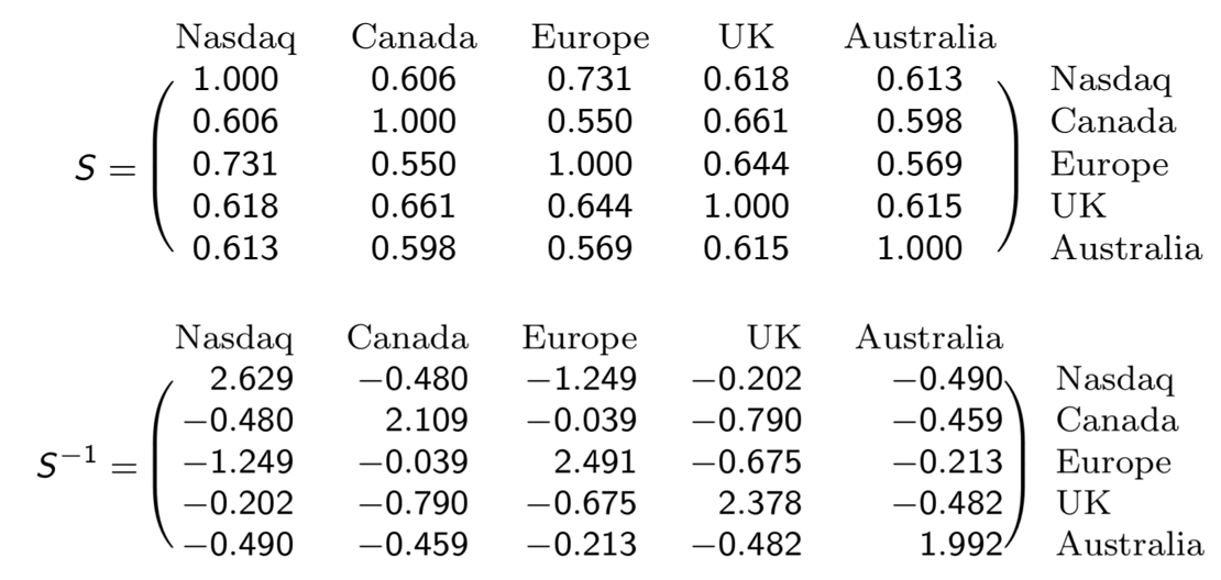
Figure 1: The sample correlation matrix of global stock market indices based on monthly returns from 2013-2016. ?Canada?, ?Europe?, ?UK?, and ?Australia? refer to the country names in the MSCI Developed Markets Index

. Notice that the covariance matrix contains all positive entries and the precision matrix is an M-matrix which implies that the joint distribution is $\text{MTP}_{2}$ (see Section 3.2 for details).

In this paper, we provide (1) a new $\text{MTP}_{2}$ covariance matrix estimator to model heavy-tailed returns data and (2) an extensive empirical comparison demonstrating the advantages of this new estimator on stock-market data spanning thirty years. The remainder of this paper is organized as follows: In Section 2 we review the Markowitz portfolio problem and existing techniques for covariance matrix estimation that we benchmark our method against in Section 5. In Section 3, we define $\text{MTP}_{2}$ more precisely, motivate its usage for financial returns data in more detail, and describe a method to perform covariance estimation under this constraint. Finally, in Section 5 we empirically compare our method with several competing methods on historical stock market data and show that covariance matrix estimation under $\text{MTP}_{2}$ outperforms state-of-the-art methods for portfolio selection in terms of out-of-sample variance, i.e. risk. All data and code for this work is available at https://github.com/uhlerlab/MTP2-finance.

2 Problem Statement

After introducing some notation, we will review the Markowitz portfolio selection problem, explain how it relates to covariance matrix estimation, and discuss various covariance estimation techniques.

2.1 Notation

We assume throughout that we are given $N$ assets, which we index using the subscript $i$, from $T$ dates (e.g. days), which we index using the subscript $t$. We let $r_{i,t}$ denote the observed return for asset $i$ at date $t$ for $1\leq i\leq N$ and $1\leq t\leq T$. The vector $r_{t}:=(r_{1,t},\ldots,r_{N,t})^{T}$ consists of the returns of each asset on day $t$. Finally, $\mu_{t}:=\mathrm{E}[r_{t}]$ and $\Sigma_{t}:=\mathrm{Cov}(r_{t})$ denote the expected returns and the covariance matrix of the returns for day $t$, respectively.

2.2 Optimal Markowitz Portfolio Allocation

Markowitz portfolio theory concerns the problem of assigning weights $w\in\mathbb{R}^{N}$ to a universe of $N$ possible assets in order to minimize the variance of the portfolio for a specified level of expected returns $R$. More precisely, the optimal portfolio weights $w\in\mathbb{R}^{N}$ on day $t$ are found by solving

$$\underset{w\in\mathbb{R}^{N}}{\text{minimize}} w^{T}\Sigma^{*}_{t}w$$ (1)

subject to $$w^{T}\mu_{t}^{*}=R\quad\textrm{and}\quad\sum_{i=1}^{N}w_{i}=1,$$

where $\mu^{*}_{t}$ and $\Sigma^{*}_{t}$ denote the true expected returns and covariance matrix of the returns for day $t$. In practice, $\mu^{*}_{t}$ and $\Sigma^{*}_{t}$ are unknown and must be estimated from historical returns. Since the main difficulty lies in estimating $\Sigma^{*}_{t}$ (it requires estimating $O(N^{2})$ parameters as compared to $O(N)$ for $\mu^{*}_{t}$), a widely used tactic to specifically evaluate the quality of a covariance matrix estimator is by finding the global minimum variance portfolio, which does not require estimating $\mu^{*}$ (Haugen and Baker, 1991; Jagannathan and Ma, 2003). Such a portfolio can be found by solving

$$\underset{w\in\mathbb{R}^{N}}{\text{minimize}} w^{T}\Sigma^{*}_{t}w$$ (2)

subject to $$\sum_{i=1}^{N}w_{i}=1,$$

where $w$ is chosen to minimize the variance of the portfolio. Replacing the unknown true covariance matrix of returns $\Sigma_{t}^{*}$ by some estimator $\hat{\Sigma}_{t}$ yields the following analytical solution for Eq. 2:

$$\hat{w}:=\frac{\widehat{\Sigma}_{t}^{-1}\mathbf{1}}{\mathbf{1}^{T}\widehat{\Sigma}_{t}^{-1}\mathbf{1}}.$$ (3)

A natural choice for $\widehat{\Sigma}_{t}$ is the sample covariance matrix. Unfortunately, as discussed in Section 1, the sample covariance matrix is a poor estimator of the true covariance matrix, particularly in the high-dimensional setting when the number of assets $N$ exceeds the number of periods $T$ (the sample size). Although the sample covariance matrix is an unbiased estimator of the true covariance matrix, in the high-dimensional setting it is not invertible, has high variance, and is not consistent (e.g., the eigenvectors of $S$ do not converge to those of $\Sigma^{*}$ (Marčenko and Pastur, 1967; Johnstone, 2001; Wachter, 1978; Bai and Yin, 1993; Johnstone et al., 2009)). Making structural assumptions about the true covariance matrix allows the construction of estimators that have lower variance with only a small increase in bias.

3 Covariance Matrix Estimation under $\text{MTP}_{2}$

We propose a new structure for modeling asset returns data, namely by exploiting that assets are often positively dependent. In particular, we consider distributions that are $\textit{MTP}_{2}$.

Definition 3.1 (Fortuin et al. (1971); Karlin and Rinott (1980b)).

A distribution on $\mathcal{X}\subseteq\mathbb{R}^{M}$ is multivariate totally positive of order 2 ($\text{MTP}_{2}$) if its density function $p$ satisfies

$$p(x)p(y)\leq p(x\wedge y)p(x\vee y)\quad\text{for all}\quad x,y\in\mathcal{X},$$

where $\wedge,\vee$ denote the coordinate-wise minimum and maximum, respectively.

$\text{MTP}_{2}$ is a strong form of positive dependence that implies most other known forms including e.g. positive association; see for example Colangelo et al. (2005) for a recent overview. Note that when $p(x)$ is a strictly positive density, then 3.1 is equivalent to $p(x)$ being log-supermodular. Log-supermodularity has a long history in ecomomics, in particular in the context of complementarity and comparative statics  (Topkis, 1978; Milgrom and Roberts, 1990; Milgrom and Shannon, 1994; Topkis, 1998; Athey, 2002; Costinot, 2009).

In Fig. 1, we provided an example of 5 global stock indices, where the sample distribution is $\text{MTP}_{2}$. To further motivate studying $\text{MTP}_{2}$ as a constraint for covariance matrix estimation for portfolio selection we discuss its connection to latent tree models in Section 3.1. In particular, we show that the capital asset pricing model implies that the resulting joint distribution is $\text{MTP}_{2}$ when all ?market betas? (also known as ?market loadings? or ?factor coefficients?) are positive. Then in Section 3.2, we discuss how to perform covariance matrix estimation under $\text{MTP}_{2}$ in the Gaussian setting. Finally, in Section 3.3, we propose how to extend this estimator to heavy-tailed distributions.

3.1 Latent Tree Models

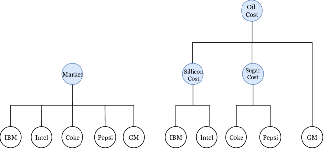
Figure 2: Shaded nodes represent factors that are potentially unobserved, and unshaded nodes are the observed returns of different companies. Figure (left) represents a simple model where an unobserved market variable drives the returns of all stocks as in the CAPM. Figure (right) represents a more complicated latent tree model where latent sector-level factors drive the returns of different assets.

A powerful framework to model complex data such as stock-market returns is through models with latent variables. Factor models, which are widely used for covariance estimation for portfolio selection (see Section 4.1) are examples thereof. A latent tree model is an undirected graphical model on a tree (where every node represents a random variable that may or may not be observed and any two nodes are connected by a unique path). For financial applications, latent tree models have been used, for example, for unsupervised learning tasks, such as clustering similar stocks, or for modeling and learning the dependence structure among asset returns (Choi et al., 2011; Mantegna, 1999). A factor analysis model with a single factor is a particular example of a latent tree model consisting of an unobserved root variable that is connected to all the observed variables; see Fig. 2 for a concrete example of a single-factor analysis model and a more general latent tree model. The prominent capital asset pricing model (CAPM) is a single-factor analysis model: the return of stock $i$ is modeled as

$$r_{i}=r_{f}+\beta_{i}(r_{m}-r_{f})+u_{i}\quad\beta_{i}\in\mathbb{R},$$

where $r_{f}$ is known as the risk-free rate of return, $r_{m}$ is the market return, and $u_{i}$ is the uncorrelated, zero mean idiosyncratic error term. Typically, the parameters $\beta_{i}$ are positive, which explains why the covariance between stock returns is usually positive. Non-negative correlation is in general necessary but not sufficient to imply $\text{MTP}_{2}$. The following theorem states that for latent tree models non-negative correlation already implies $\text{MTP}_{2}$. The proof follows from Lauritzen et al. (2019a, Theorem 5.4).

Theorem 3.2.

Let $X\in\mathbb{R}^{M}$ follow a multivariate Gaussian distribution that factorizes according to a tree. If $\mathrm{Cov}(X)\geq 0$, then $X$ is $\text{MTP}_{2}$ and any marginal of $X$ is $\text{MTP}_{2}$.

While working with CAPM is convenient from a theoretical perspective, its simplicity often comes at the expense of underfitting. In particular, there commonly are additional sector-level factors that drive returns. Identifying these factors is an active area of research; for instance, CAPM was recently extended to include three and then five new factors French and French (1993); Fama and French (2015). However, identifying relevant factors is in general a challenging task; for example, learning the structure of a latent tree model from data is known to be NP-hard (Cooper, 1990). We here propose to instead take a structure-free approach by constraining the joint distribution over the observed variables to be $\text{MTP}_{2}$. This approach provides more flexibitlity than modeling stock returns using latent tree models and at the same time allows overcoming the computational bottleneck of fitting a latent tree model. In particular, we show in Section 3.2 that an $\text{MTP}_{2}$ covariance matrix estimator can be computed by solving a convex optimization problem.

3.2 $\text{MTP}_{2}$ Covariance Matrix Estimation Assuming Multivariate Gaussian Returns

For multivariate Gaussian distributions, a necessary and sufficient condition for a distribution to be $\text{MTP}_{2}$ is that the precision matrix $K\coloneqq\Sigma^{-1}$ is an M-matrix, i.e., $K_{ij}\leq 0$ for all $i\neq j$; or equivalently, all partial correlations are nonnegative. (Karlin and Rinott, 1980a). Following Lauritzen et al. (2019a), we consider the maximum likelihood estimator (MLE) of $K$ subject to $K$ being an M-matrix.

Recall that the log-likelihood function $\mathcal{L}$ of $K$ given data $D\coloneqq\{r_{t}\}_{t=1}^{T}\overset{\text{i.i.d.}}{\sim}N(0,K)$ is, up to additive and multiplicative constants, given by

$$\mathcal{L}(K;D)=\log\det K-\text{trace}(KS),$$ (4)

where $S\in\mathbb{R}^{N\times N}$ denotes the sample covariance matrix of the returns $\{r_{t}\}_{t=1}^{T}$ or log-returns. Without the $\text{MTP}_{2}$ constraint, the MLE of $K$ is obtained by maximizing $\mathcal{L}(K;D)$ over the set of all positive semidefinite matrices and is given by $S^{-1}$ when $N\leq T$ (i.e., the dimension of the covariance matrix is less than the number of samples). Note that when $N\geq T$, the MLE does not exist, i.e., the log-likelihood function is unbounded above. Remarkably, by adding the constraint that $K$ is an M-matrix (i.e., that the distribution is $\text{MTP}_{2}$), then the MLE

$$\hat{K}=\arg\max_{K\succeq 0}\ \log\det K-\text{trace}(KS)\quad\text{subject to}\quad K_{ij}\leq 0\quad\forall i\neq j,$$ (5)

exists with probability 1 when $T\geq 2$ for any dimension $N$ Slawski and Hein (2014); Lauritzen et al. (2019a). Similarly, the popular CLIME estimator, which we review in Eq. (10) in the next section, could be extended to the MTP₂ setting by adding the constraints $K_{ij}\leq 0$ for all $i\neq j$. It would be of interest to understand its properties.

The fact that a unique solution exists for Eq. 5 for any $N$ when $T\geq 2$ suggests that the $\text{MTP}_{2}$ constraint adds considerable regularization for covariance matrix estimation. In addition, the problem in Eq. 5 is a convex optimization problem and computationally efficient coordinate-descent algorithms have been described for computing $\hat{K}$ (cf. Lauritzen et al., 2019a; Slawski and Hein, 2014). Finally, another desirable property is that the $\text{MTP}_{2}$ covariance matrix estimator $\hat{K}$ in Eq. 5 is usually sparse (Lauritzen et al., 2019a, Corallary 2.9), which reduces the intrinsic dimensionality of the model and hence reduces the variance of the estimator. Note that this sparsity is achieved without the need of any tuning parameter, an immediate advantage over methods that explicitly add sparsity-inducing $L_{1}$ penalties such as the graphical lasso (Friedman et al., 2008; Ravikumar et al., 2011) discussed in Section 4.3. Nevertheless, to relax the $\text{MTP}_{2}$ constraint, one could always introduce a Lagrange multiplier (i.e., tuning parameter) to penalize for violating the $\text{MTP}_{2}$ constraint.

3.3 Extensions to Heavy-Tailed Distributions

Asset returns are often computed as $r_{t}=\log\left(\frac{p_{t}}{p_{t-1}}\right)$, where $p_{t}$ is the price of the asset at time $t$. Stock returns may be heavy tailed, and in such cases the Gaussian assumption made for estimating the covariance matrix in Section 3.2 may be problematic. Transelliptical distributions form a convenient class of distributions that contain the Gaussian distribution as well as heavy-tailed distributions such as the $t$-distribution. In the following, we provide an extension of the estimator in Eq. 5 to transelliptical distributions.

A random vector $X$ with density function $p(x)$, mean $\mu\in\mathbb{R}^{M}$ and covariance matrix $\Sigma\in\mathbb{R}^{M\times M}$ follows an elliptical distribution if its density function can be expressed as

$$g((x-\mu)^{T}\Sigma^{-1}(x-\mu))$$

for some function $g$. More generally, $X$ follows a transelliptical distribution if there exist monotonically increasing functions $f_{i}$, $i=1,\dots,M$, such that $(f_{1}(X_{1}),\cdots,f_{M}(X_{M}))$ follows an elliptical distribution. We denote the covariance matrix of this elliptical distribution by $\Sigma_{f}$. The following result provides a necessary condition for a transelliptical distribution to be $\text{MTP}_{2}$.

Theorem 3.3.

Suppose that the joint distribution of $(X_{1},\cdots,X_{M})$ is $\text{MTP}_{2}$ and transelliptical, i.e., there exist increasing functions $f_{i}$, $i=1,\dots,M$, such that the density function of $(f_{1}(X_{1}),\cdots,f_{M}(X_{M}))$ can be written as $g((x-\mu)^{T}\Sigma_{f}^{-1}(x-\mu))$. Then, $\Sigma_{f}^{-1}$ is an M-matrix.

We prove 3.3 in A. While 3.3 shows that the covariance matrix of any elliptical distribution is an inverse M-matrix, the following example shows that, unlike in the Gaussian setting, this is not a sufficient condition for $\text{MTP}_{2}$.

Example 3.4.

Suppose $X$ is a two-dimensional $t$-distribution with one degree of freedom and precision matrix

$$\Sigma^{-1}=\begin{bmatrix}1&-0.1\\ -0.1&1\\ \end{bmatrix}.$$

Then $X$ is not $\text{MTP}_{2}$, since for $x=(-1,1)$ and $y=(0,0)$ its density function $p(\cdot)$ satisfies $p(x)p(y)>p(x\wedge y)p(x\vee y)$. ∎

This shows that for transelliptical distributions, the constraint that $\Sigma^{-1}$ be an M-matrix is a relaxation of $\text{MTP}_{2}$. In terms of covariance matrix estimators for transelliptical distributions (without the $\text{MTP}_{2}$ constraint), it was shown recently that replacing the sample covariance matrix $S$ in Eq. 9 and Eq. 10 by Kendall’s tau correlation matrix $S_{\tau}$ defined in Eq. 11 yields consistent estimators of $\Sigma_{f}$ (Liu et al., 2012; Barber and Kolar, 2018). This is quite remarkable, since it does not involve any changes to the objective function apart from replacing $S$ by $S_{\tau}$. Motivated by these results, we propose to extend the $\text{MTP}_{2}$ covariance matrix estimator from Section 3.2 to heavy-tailed distributions using the covariance matrix estimator in Eq. 5 by simply replacing the sample covariance matrix $S$ by $S_{\tau}$.

In recent work, Rossell and Zwiernik (2020) provide a number of interesting theoretical results for transelliptical distributions, including the theoretical analysis of our proposed $\text{MTP}_{2}$ relaxation above. They show that our relaxation for transelliptical distributions has a number of desirable properties, including positive partial correlations for arbitrary conditioning sets and the avoidance of Simpsons Paradox; see (Rossell and Zwiernik, 2020, Proposition 4.12) for details. Rossell and Zwiernik (2020) further motivate this relaxation by showing that $\text{MTP}_{2}$ is in fact too strong of a constraint for (non-Gaussian) transelliptical distributions in Theorem 4.8 (for example, there does not exist any transelliptical $\text{MTP}_{2}$ $t$-distributions).

4 Related Work

In this section, we review several models and techniques for covariance matrix estimation that are commonly used in financial contexts. We compare our method to these estimators in Section 5.

4.1 Factor Models

A common modeling assumption in financial applications is that the returns for day $t$ are given by a linear combination of a (small) collection of latent factors $f_{k,t}$ for $1\leq k\leq K$, which are either explicitly provided or estimated from the data. In such a factor model, the returns are modeled as

$$r_{i,t}=\alpha_{i}+\beta_{i}^{T}f_{t}+u_{i,t},\quad f_{t}:=(f_{1,t},\ldots,f_{K,t}),$$ (6)

where $u_{i,t}$ is the idiosyncratic error term for asset $i$ that is uncorrelated with $f_{t}$. Letting $B\in\mathbb{R}^{K\times N}$ be the matrix whose $i$th column is $\beta_{i}$, the covariance matrix of the returns can be expressed as

$$\Sigma_{t}=B^{T}\Sigma_{f,t}B+\Sigma_{u,t},\quad\text{for}\quad 1\leq t\leq T,$$

where $\Sigma_{f,t}:=\mathrm{Cov}(f_{t})$ and $\Sigma_{u,t}:=\mathrm{Cov}(u_{t})$. In practice, $K\ll N$ factors are selected, making $B^{T}\Sigma_{f,t}B$ low-rank. This low-rank structure makes estimating $\Sigma_{t}$ easier since $\Sigma_{f,t}$ and $B$ only have $O(K^{2})$ and $O(NK)$ free parameters, respectively. When $K\ll N$, and $K\ll T^{2}$, then by standard concentration of measure results, $\Sigma_{f,t}$ can be estimated well by $\widehat{\Sigma}_{f,t}$, the sample covariance matrix of the factors. Similarly, by Eq. 6, the $i$th row of $B$ can be estimated by regressing the returns of asset $i$ on the $K$ latent factors, for example using ordinary least-squares. In this case, $\hat{\beta}_{i}\approx\beta_{i}$ and hence the error $u_{i,t}$ is approximately equal to the residual $\hat{u}_{i,t}\coloneqq r_{i,t}-\hat{\beta}_{i}^{T}f_{t}-\hat{\alpha}_{i}$. Thus $\Sigma_{u,t}$ can be approximated by a covariance matrix estimate $\hat{\Sigma}_{u,t}$ based on the residuals. However, without additional assumptions on the structure of $\Sigma_{u,t}$, $\Sigma_{u,t}$ is not necessarily easier to estimate than $\Sigma_{t}$. As a result, many estimators assume that $\Sigma_{u,t}$ has some special structure such as being diagonal or sparse (see below).

Several different types of factor models of varying complexity have been considered in the literature: The general model in Eq. 6 is known as a dynamic factor model. A static factor model assumes that the covariance matrices $\Sigma_{u,t}$ and $\Sigma_{f,t}$ are time-invariant, i.e., $\Sigma_{u,t}=\Sigma_{u}$ and $\Sigma_{f,t}=\Sigma_{f}$ do not depend on $t$. An exact factor model furthermore assumes that the covariance matrix $\Sigma_{u}$ is diagonal, whereas an approximate factor model assumes that $\Sigma_{u}$ has bounded $L^{1}$ or $L^{2}$ norm. In this paper, we concentrate on static estimators. The following static factor-based covariance matrix estimators are popularly used in financial applications.

• POET: is based on an approximate factor model and was first proposed in Fan et al. (2013). POET estimates $B^{T}\Sigma_{f,t}B$ by a rank $K$ truncated singular value decomposition (SVD) of the sample covariance matrix $\hat{\Sigma}$, which we denote by $\hat{\Sigma}_{K}$. $\widehat{\Sigma}_{u}$ is estimated by soft-thresholding the off-diagonal entries of the residual covariance matrix $S_{\hat{u}}=\hat{\Sigma}-\hat{\Sigma}_{K}$ based on the method in Bickel and Levina (2008).

• EFM: is an estimator based on the exact factor model using the Fama-French factors (Fama and French, 1993). $\widehat{\Sigma}_{f}$ equals the sample covariance matrix of the factors $\{f_{t}\}$ and $\widehat{\Sigma}_{u}$ equals the diagonal of $S_{\hat{u}}$.

• AFM-POET: is an estimator based on an approximate factor model using the Fama-French factors. $\widehat{\Sigma}_{f}$ is obtained as in EFM, whereas $\widehat{\Sigma}_{u}$ is obtained by soft-thresholding $S_{\hat{u}}$ as in POET.

4.2 Shrinkage of Eigenvalues

Another way to impose structure on the covariance matrix is through assumptions on the eigenvalues of the covariance matrix. Assuming that the true covariance matrix is well-conditioned, then the extreme eigenvalues of the sample covariance matrix are generally too small/large as compared to the true covariance matrix (Marčenko and Pastur, 1967; Bai and Yin, 1993). This motivates the development of covariance matrix estimators such as linear shrinkage Ledoit and Wolf (2004) and extensions thereof  (cf. Ledoit and Wolf, 2012; Engle et al., 2017) that shrink the eigenvalues of the sample covariance matrix for better statistical properties.

To be more precise, let

$$S=\sum_{i=1}^{N}\lambda_{i}v_{i}v_{i}^{T},$$

be the eigendecomposition of the sample covariance matrix $S$, where $\lambda_{i}$ denotes the $i$-th eigenvalue of $S$ and $v_{i}$ the corresponding eigenvector. Then the linear shrinkage estimator is given by

$$\widehat{\Sigma}_{LS}=\sum_{i=1}^{N}\gamma_{i}v_{i}v_{i}^{T},$$

where $\gamma_{i}=\rho\lambda_{i}+(1-\rho)\bar{\lambda}$ with $\bar{\lambda}$ denoting the average of the eigenvalues of $S$ and $0<\rho<1$ a tuning parameter that determines the amount of shrinkage. Note that $\widehat{\Sigma}_{LS}$ can equivalently be expressed as

$$\widehat{\Sigma}_{LS}=\rho S+(1-\rho)\bar{\lambda}I_{N},$$ (7)

where $I_{N}\in\mathbb{R}^{N\times N}$ denotes the identity matrix (Eq. (7) follows from the uniqueness of the eigenvalue decomposition). Thus $\widehat{\Sigma}_{LS}$ is obtained by shrinking the sample covariance matrix towards a multiple of the identity, which from a Bayesian point of view can also be interpreted as using the identity matrix as a prior for the true covariance matrix (Ledoit and Wolf, 2004). The shrinkage estimator $\widehat{\Sigma}_{LS}$ is asymptotically efficient given a particular choice of $\rho$ that depends on the sample covariance matrix $S$, its dimension $N$ (i.e., the number of assets) and the number of samples $T$ (i.e., the number of dates) (Ledoit and Wolf, 2004).

An extension of linear shrinkage, known as non-linear shrinkage, considers non-linear transforms of the eigenvalues according to the Marcenko-Pastur distribution, which describes the asymptotic distribution of the eigenvalues of random matrices. This approach has been shown to outperform linear-shrinkage empirically (Ledoit and Wolf, 2012). It is also common to combine shrinkage estimators with factor models (e.g., such as those introduced in Section 4.1). For example, AFM-LS and AFM-NLS apply linear shrinkage and non-linear shrinkage, respectively, to the residuals (by regressing out the Fama-French factors) to estimate $\Sigma_{u}$ (De Nard et al., 2018).

4.3 Regularization of the Precision Matrix

Another common technique for covariance matrix estimation is to assume that the true underlying inverse covariance matrix $K^{*}:=(\hat{\Sigma}^{*})^{-1}$, also known as the precision matrix, is sparse, i.e. that the number of non-zero entries in $K^{*}$ is bounded by an integer $\kappa>0$. Since estimating $K$ under the constraint

$$\|K\|_{0}\coloneqq\sum_{i\neq j}I[K_{ij}\neq 0]\leq\kappa$$ (8)

is computationally intractable as it involves solving a difficult combinatorial optimization problem, a standard approach is to replace the $L_{0}$ constraint in Eq. 8 by an $L_{1}$ constraint. In particular, assuming that the data follows a multivariate Gaussian distribution, then the $L_{1}$-regularized maximum likelihood estimator (also known as graphical lasso) can be used to estimate $K$ (Friedman et al., 2008; Ravikumar et al., 2011). Maximum likelihood estimation under the the $L_{1}$ constraint leads to the following convex optimization problem:

$$\hat{K}\coloneqq\operatorname*{arg\,max}_{K\succeq 0}\ \log\det K-\text{trace}(KS)\quad\text{subject to}\quad\|K\|_{1}\leq\lambda,$$ (9)

where $\lambda\geq 0$ is a tuning parameter. Instead of maximizing the log-likelihood, the popular CLIME estimator Liu et al. (2012) finds a sparse estimate of the precision matrix by solving

$$\hat{K}\coloneqq\operatorname*{arg\,min}_{K}\|K\|_{1}\quad\text{subject to}\quad\|SK-I_{N}\|_{\infty}\leq\lambda.$$ (10)

and has similar consistency guarantees as the graphical lasso in the Gaussian setting.

To overcome the restrictive Gaussian assumption, recent work suggested replacing the sample covariance matrix $S$ in Eq. 9 and Eq. 10 by Kendall’s tau correlation matrix $S_{\tau}$ with $(S_{\tau})_{ij}\coloneqq\sin(\frac{\pi}{2}\hat{\tau})$, where

$$\hat{\tau}_{ij}\coloneqq\frac{1}{{T\choose 2}}\sum_{1\leq t\leq t^{\prime}\leq T}\text{sign}(X_{it}-X_{it^{\prime}})\ \text{sign}(X_{jt}-X_{jt^{\prime}}).$$ (11)

Interestingly, the resulting estimators can also be used for data from heavy-tailed distributions (including elliptical distributions such as the $t$-distribution) with almost no loss in efficiency (Liu et al., 2012; Barber and Kolar, 2018); see also Section 3.3.

5 Empirical Evaluation

In this section, we first describe both the data used for the evaluation and our experimental setup, which closely follows De Nard et al. (2018) for reproducibility. We then present our empirical evaluation of the various methods discussed in this paper based on the global minimum variance portfolio problem and the full Markovitz portfolio problem. All data and code for this work is available at https://github.com/uhlerlab/MTP2-finance.

5.1 Data

We use daily stock returns data from the Center for Research in Security Prices (CRSP), starting in 1975 and ending in 2015. We restrict our attention to stocks from the NYSE, AMEX and NASDAQ stock exchanges, and consider different portfolio sizes $N\in\{100,200,500\}$. As in De Nard et al. (2018), $21$ consecutive trading days constitute one ‘month’. To account for distribution shift over time, we use a rolling out-of-sample estimator. That is, for each month in the out-of-sample period, we estimate the covariance matrix using the most recent $T$ daily returns, and update the portfolio monthly. We vary $T$ with $N$ to evaluate how sensitive different covariance estimators are with respect to increasing dimensionality. In particular, for a given $N$, we vary $T$ such that the ratio $N/T\in\{\frac{1}{2},1,2,4\}$. We also include $T=1260$ (which corresponds to 5 years of market data) in order to replicate the results in De Nard et al. (2018). We consider 360 months for evaluation, starting from 01/08/1986 and ending on 12/02/2015, using the portfolio and covariance updating strategy described above. We index each of these 360 investment periods by $h\in\{1,\ldots,360\}$.

For each investment period and portfolio size, we vary the investment universe because many stocks do not have data for the entire period and the most relevant stocks (i.e. by market capitalization or volume) naturally vary over time. We use the same procedure as in De Nard et al. (2018) to construct the investment universe. Specifically, we consider the set of stocks that have (1) an almost complete return history over the most recent $T=1260$ days and (2) a complete return ‘future’ in the next 21 days (which is the investment period). Next, we remove one stock in each pair of highly correlated stocks, defined as those with sample correlation exceeding $0.95$. More precisely, for each pair we remove the stock with the lower market capitalization for period $h$. Finally, we pick the largest $N$ stocks (as measured by their market capitalization on the investment date $h$) for the subsequent analysis. We use $I_{h,N}$ to denote this investment universe, where the subscripts emphasize the dependence on $N$ and $h$.

5.2 Competing Covariance Matrix Estimators

We compare the performance of the proposed MTP₂ covariance matrix estimator to the estimators described in Section 4. In addition, as a baseline, we also consider the equally weighted portfolio denoted by $\mathbf{1/N}$. We evaluate each estimator in terms of its out-of-sample standard deviation (see Section 5.3), Sharpe ratio (see Section 5.4), and information ratio (see B). These results are also summarized in Table 1 and Table 2. In the following, we provide details regarding the implementation of the various covariance matrix estimators included in our empirical analysis.

• LS: linear shrinkage, as described in Section 4.2, applied to the sample covariance matrix.

• NLS: non-linear shrinkage, as described in Section 4.2, applied to the sample covariance matrix; we used the implementation in the R package shrink (Dunkler et al., 2016).

• AFM-LS: approximate factor model, as described in Section 4.1, with $5$ Fama-French factors and linear shrinkage applied to estimate the covariance matrix of the residuals.

• AFM-NLS: approximate factor model, as described in Section 4.1, with $5$ Fama-French factors and non-linear shrinkage applied to estimate the covariance matrix of the residuals.

• POET (k=3): POET, as described in Section 4.1, using the top $3$ principal components; we used the implementation in the R package POET.

• POET (k=5): POET, as described in Section 4.1, using the top $5$ principal components; we used the implementation in the R package POET.

• GLASSO: graphical lasso, as described in Section 4.3, using the python implementation in sklearn (Pedregosa et al., 2011); cross-validation is used to select the hyperparameter $\lambda$; we used the default parameters, i.e. using 3-fold cross-validation and testing $\lambda$ on a grid of 4 points refined 4 times (the parameter values for $\alpha$ and $n_{\text{iter}}$ respectively). We note that this results in a biased estimator due to the $\ell_{1}$-penalty.

• CLIME: as described in Section 4.3; we used the implementation in the R package CLIME with hyperparameter $\lambda=\sqrt{(\log p)/n}$, which is asymptotically optimal; the CLIME estimator using this hyperparameter only exists when $T\geq N$ and hence we only benchmarked CLIME in this range.

• CLIME-KT: CLIME estimator as described above but using Kendall’s tau correlation matrix instead of the sample correlation matrix. Since Kendall’s tau correlation matrix is not singular, the CLIME-KT estimator exists even when when $T\leq N$.

• MTP2: our method, as described in Section 3.2. We used the implementation from Slawski and Hein (2014), which is a computationally efficient coordinate-descent algorithm implemented in Matlab.

• MTP2-KT: MTP2 estimator as described above but using Kendall’s tau correlation matrix instead of the sample correlation matrix; see Section 3.3.

5.3 Evaluation on the Global Minimum Variance Portfolio Problem

For each fixed portfolio size $N$, estimation sample size $T$, and investment period $h$, we let $\widehat{\Sigma}^{\mathcal{M}}_{T,h}(I_{h,N})$ denote the estimated covariance matrix between the assets in universe $I_{h,N}$ obtained using estimator $\mathcal{M}$. We then computed the portfolio weights $\hat{w}^{\mathcal{M}}_{h}$ via Eq. 3 and the corresponding returns $r^{\mathcal{M}}_{h}$ for $h=1,\dots,360$. We estimated the portfolio standard deviation from these 360 returns for each estimator and multiplied each standard deviation by $\sqrt{12}$ to annualize. Note that a smaller standard deviation implies a lower variance portfolio, and hence better empirical performance.

N	T	1/N	LS	NLS	AFM-	AFM-	POET	POET
					LS	NLS	(k=3)	(k=5)
100	50	18.724	13.452	12.976	13.159	13.193	12.498*	12.617
	100	18.724	13.695	13.111	13.135	13.338	11.994*	12.595
	200	18.724	12.560	12.347	12.357	12.480	12.348	12.707
	400	18.724	12.451	12.347	12.352	12.344	12.744	13.255
	1260	18.724	12.151	12.122	12.146	12.130	13.041	12.722
200	100	18.134	12.583	12.320	12.372	12.406	11.743	11.544
	200	18.134	11.881	11.603	11.556	11.612	11.881	11.593
	400	18.134	11.656	11.431*	11.552	11.469	12.559	12.103
	800	18.134	11.670	11.424*	11.531	11.449	13.019	12.455
	1260	18.134	11.665	11.534*	11.601	11.568	13.170	12.898
500	250	17.925	11.140	10.516	10.508	10.517	11.269	10.203*
	500	17.925	11.934	10.793*	10.913	11.163	11.833	10.873
	1000	17.925	11.373	10.838	10.856	10.816*	12.179	11.917
	1260	17.925	11.469	10.943*	11.005	10.950	12.395	11.626

N	T	GLASSO	CLIME	CLIME-	MTP2	MTP2-
				KT		KT
100	50	13.594	nan	15.484	12.655	12.623
	100	13.822	nan	15.024	12.327	12.049
	200	13.985	14.945	15.140	11.858	11.742*
	400	13.607	15.127	15.223	12.294	12.114*
	1260	13.631	15.253	15.316	12.087*	12.087*
200	100	13.522	nan	14.983	11.803	11.445*
	200	13.719	nan	14.344	11.586	11.442*
	400	13.920	14.563	14.964	11.880	11.905
	800	14.096	14.778	14.862	11.635	11.661
	1260	13.958	15.013	15.013	11.710	11.749
500	250	13.855	nan	15.677	10.455	10.512
	500	14.171	nan	20.896	11.009	11.261
	1000	14.283	15.523	14.330	11.031	11.273
	1260	14.290	14.776	14.962	11.187	11.422

Table 1: For each combination of $N$ (portfolio size), $T$ (estimation sample size), and covariance matrix estimator, we report the out-of-sample standard deviation of the returns of the portfolio. The most competitive value in each row is marked with an asterisk.

Table 1 summarizes the results for each estimator. Each row corresponds to a particular choice of $N$ (size of investment universe) and $T$ (estimation sample size). Each column corresponds to a different covariance matrix estimator. The best performing estimator in each row is marked with an asterisk. While no estimator outperforms all other estimators across all $N$ and $T$, Table 1 shows that the MTP2, non-linear shrinkage (NLS), and POET estimators perform consistently well in all settings.

As discussed in Section 3.3, to deal with the heavy-tailed nature of the distribution of returns, Kendall’s tau correlation matrix can be used instead of the sample correlation matrix in the CLIME and MTP2 estimators which assume Gaussianity. Columns CLIME-KT and MTP2-KT in Table 1 indicate that while using Kendall’s tau correlation matrix usually does not make a significant difference in the performance, it can give a slight boost for the MTP2 estimator in particular when $N$ is 100 or 200.

Instead of comparing the covariance matrix estimators only based on one number, the standard deviation of the returns of the resulting portfolios across the entire out-of-sample period, it is also of interest to examine the performance of each estimator throughout the out-of-sample period. Figure 3 shows the standard deviation of the returns of the different estimators for $N\in\{100,200,500\}$ and $T=1260$ when varying the out-of-sample period from 60 to $360$ (where $360$ is the maximal number of total out-of-sample months). Note that the ordering between the different estimators is relatively consistent over time, indicating that the conclusions from the comparison of the different estimators in Table 1 would remain unchanged even when varying the length of the out-of-sample period.

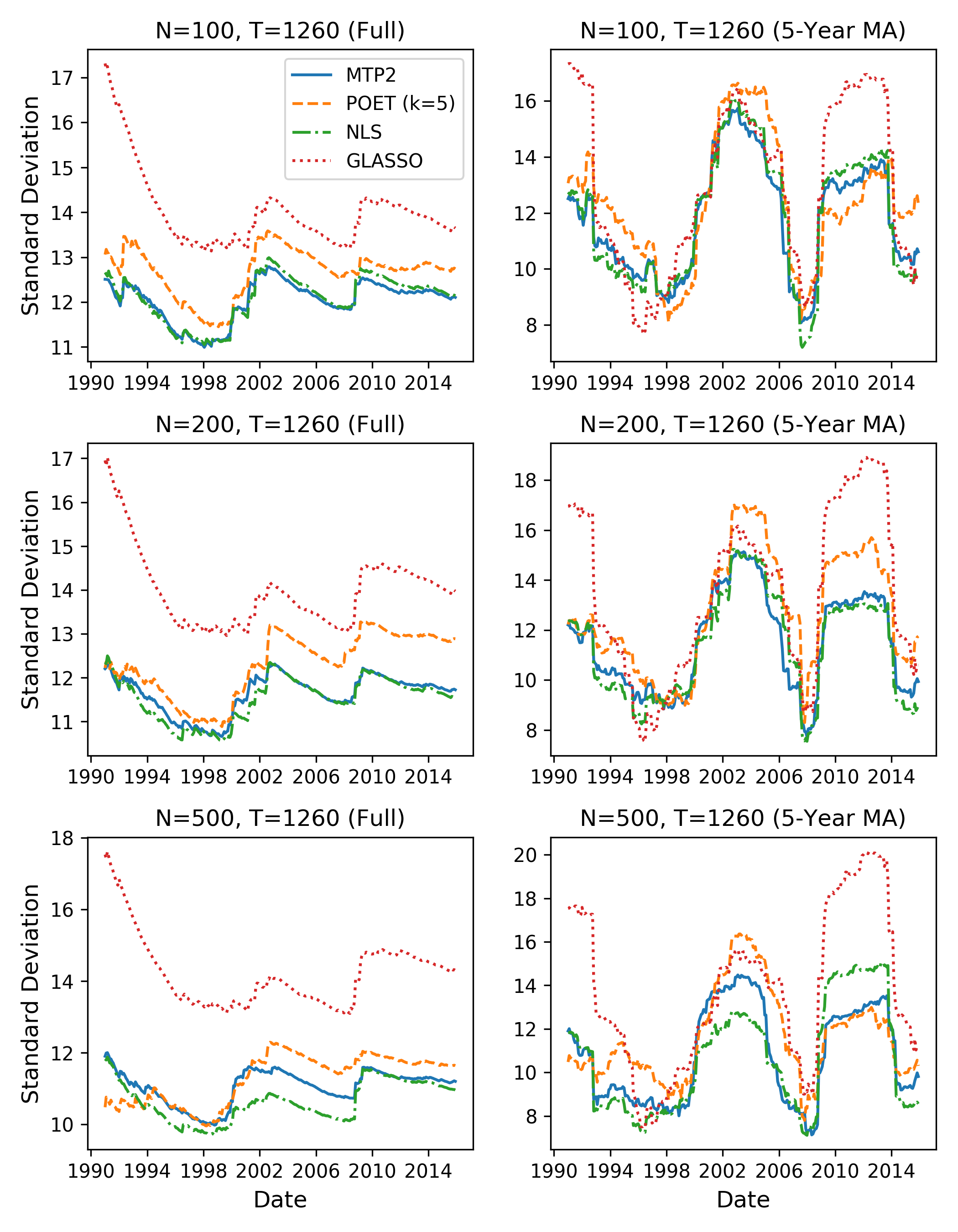
Figure 3: By varying the length of the out-of-sample period we examine the standard deviation of the returns obtained by each estimator throughout time. ?Full? is the cumulative average while ?5-Year MA? is a 5 year moving average. Lower is better.

5.4 Evaluation on Full Markowitz Portfolio Problem with Momentum Signal

We also benchmarked the different covariance matrix estimators based on the performance of the portfolios selected by solving Eq. 1, where $\Sigma^{*}_{t}$ is replaced by the estimator. A standard performance metric is the Sharpe ratio, which is the ratio between the excess portfolio returns and the standard deviation of excess returns. Hence, a higher Sharpe ratio indicates better performance.

N	T	EQ-TW	LS	NLS	AFM-	AFM-	POET	POET
					LS	NLS	(k=3)	(k=5)
100	50	0.544	0.348	0.361	0.334	0.338	0.462	0.496
	100	0.544	0.328	0.397	0.344	0.340	0.486	0.394
	200	0.544	0.374	0.419	0.389	0.376	0.500	0.413
	400	0.544	0.437	0.471	0.502	0.475	0.532	0.474
	1260	0.544	0.525	0.527	0.526	0.524	0.555	0.539
200	100	0.599	0.423	0.433	0.413	0.428	0.448	0.439
	200	0.599	0.498	0.471	0.474	0.468	0.432	0.443
	400	0.599	0.545	0.559	0.566	0.568	0.528	0.513
	800	0.599	0.649	0.636	0.640	0.643	0.461	0.571
	1260	0.599	0.588	0.585	0.593	0.585	0.491	0.481
500	250	0.599	0.649	0.639	0.641	0.638	0.538	0.664
	500	0.599	0.628	0.609	0.653	0.668	0.534	0.685
	1000	0.599	0.592	0.633	0.650	0.636	0.470	0.550
	1260	0.599	0.595	0.628	0.646	0.642	0.505	0.589

N	T	GLASSO	CLIME	CLIME-	MTP2	MTP2-
				KT		KT
100	50	0.589	nan	0.548	0.554	0.611*
	100	0.616	nan	0.589	0.594	0.666*
	200	0.589	0.580	0.636*	0.585	0.634
	400	0.603	0.608	0.578	0.590	0.617*
	1260	0.605*	0.535	0.523	0.582	0.547
200	100	0.611*	nan	0.593	0.514	0.594
	200	0.587	nan	0.632*	0.563	0.594
	400	0.597	0.657*	0.568	0.573	0.581
	800	0.596	0.605	0.552	0.650*	0.627
	1260	0.620	0.593	0.632	0.638*	0.615
500	250	0.639	nan	0.341	0.755	0.779*
	500	0.623	nan	0.313	0.705*	0.674
	1000	0.637	0.572	0.818*	0.723	0.635
	1260	0.635	0.585	0.539	0.701*	0.635

Table 2: For each combination of $N$ (portfolio size), $T$ (estimation sample size), and covariance matrix estimator, we report the out-of-sample Sharpe ratio (the ratio between the excess portfolio returns and the standard deviation of excess returns based on 1 Year US Treasury Rates). The most competitive value in each row is marked with an asterisk.

We selected the desired expected returns level $R$ as in De Nard et al. (2018). Namely, we considered the EW-TQ portfolio which places equal weight on each of the top $20\%$ of assets (based on expected returns). We then set $R$ equal to the expected return of the EW-TQ portfolio. In addition, since the true vector of expected returns $\mu^{*}$ is unknown, we estimated it from the data. We do this using the momentum factor (Jegadeesh and Titman, 1993) as in De Nard et al. (2018), which for a given investment period $h$ and stock is the geometric average of returns of the previous year excluding the past month.

The out-of-sample Sharpe ratio and information ratio of each estimator are shown in Table 2 and B, respectively. As in Table 1, each row corresponds to a different choice of $N$ and $T$ and each column corresponds to a different estimator for both tables. The best performing estimator in each row is marked with an asterisk. This analysis shows that the MTP2 estimator achieves the best performance for almost all choices of $N$ and $T$. Although the results are similar, comparing MTP2 to MTP2-KT indicates that it is recommended to use Kendall’s tau correlation matrix instead of the sample correlation matrix with the MTP2 estimator when $N$ is 100 or 200.

Similar to Figure 3, in Figure 4 we show the Sharpe ratio of the returns of the different estimators for $N\in\{100,200,500\}$ and $T=1260$ when varying the out-of-sample period from 60 to $360$. Note that while the ordering between the different estimators is still relatively consistent over time, it varies more than for the standard deviation plotted in Figure 3 and could provide additional valuable information regarding each estimator that is not captured in Table 2.

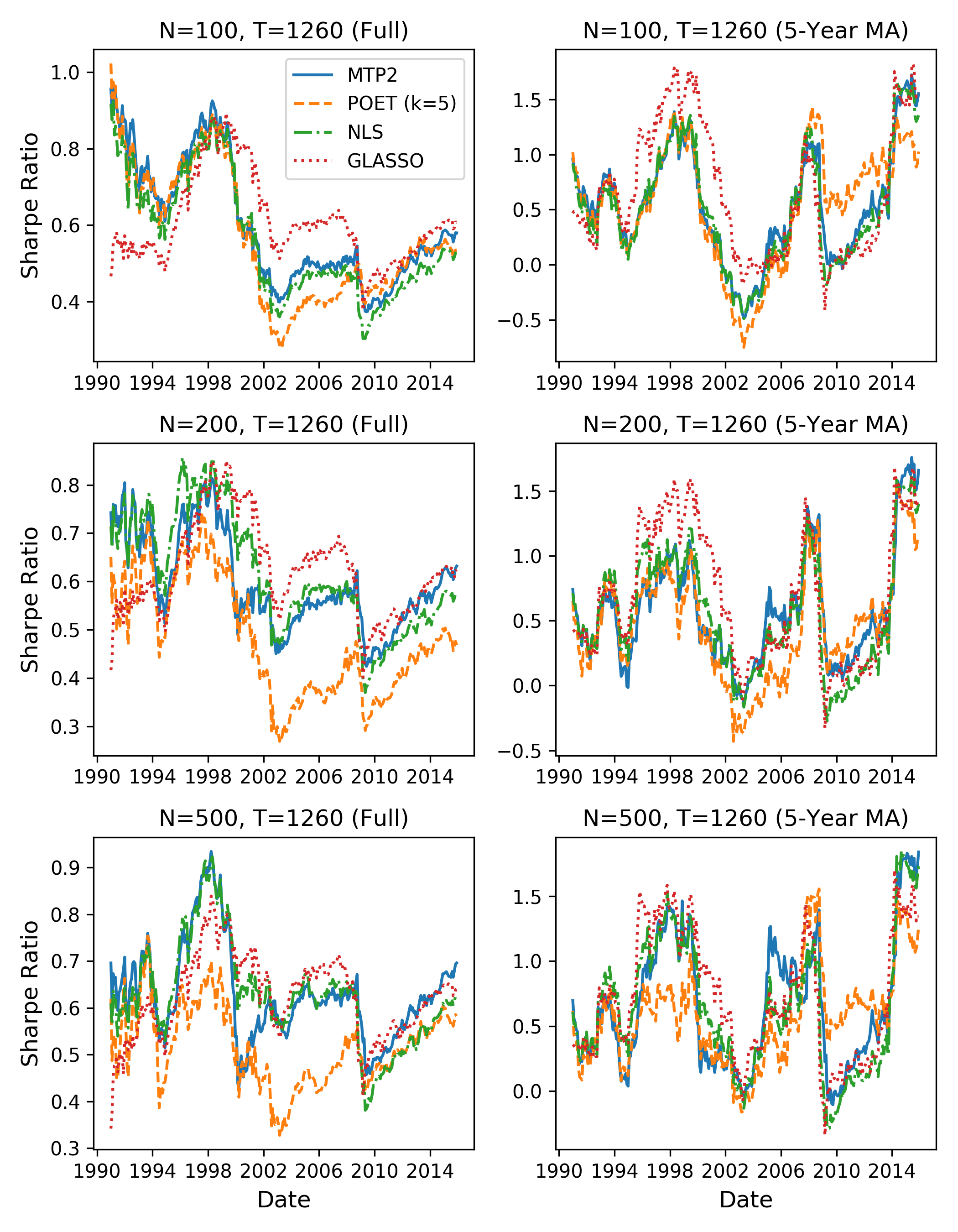
Figure 4: By varying the length of the out-of-sample period we examine the Sharpe ratio of the returns obtained by each estimator throughout time. ?Full? is the cumulative average while ?5-Year MA? is a 5 year moving average. Higher is better.

6 Conclusion

In this paper, we proposed a new covariance matrix estimator for portfolio selection based on the assumption that returns are $\text{MTP}_{2}$, which is a strong form of positive dependence. While the $\text{MTP}_{2}$ assumption is strong, this constraint adds considerable regularization, thereby reducing the variance of the resulting covariance matrix estimator. Empirically, the added bias of $\text{MTP}_{2}$ is outweighed by the reduction in variance. In particular, the proposed $\text{MTP}_{2}$ estimator outperforms previous state-of-the-art covariance matrix estimators in terms of the Sharpe ratio and the information ratio.

In our empirical evaluation we observed that using Kendall tau’s correlation matrix instead of the sample covariance matrix in the MLE under MTP₂ performed particularly well for a portfolio size of 100 or 200. It would therefore be of interest to analyze the theoretical properties of such covariance matrix estimators including MLE or CLIME under MTP₂ for heavy-tailed distributions. In addition, while we only considered static covariance matrix estimators in this paper, the $\text{MTP}_{2}$ estimator naturally extends to the dynamic setting, where the covariance matrix evolves over time. Specifically, we may adapt the techniques developed in Engle et al. (2017) to obtain a dynamic estimator under $\text{MTP}_{2}$. In future work, it would be interesting to compare the resulting estimator to other state-of-the-art dynamic covariance matrix estimators. Another interesting future direction is the theoretical analysis of the spectrum of symmetric M-matrices in the high-dimensional setting. If the $\text{MTP}_{2}$ constraint already implicitly regularizes the spectrum sufficiently, then shrinkage methods such as those developed in Ledoit and Wolf (2004, 2012); Engle et al. (2017); Jagannathan and Ma (2003); DeMiguel et al. (2013) may be unnecessary under $\text{MTP}_{2}$. Alternatively, covariance matrix estimators under $\text{MTP}_{2}$ could be combined with shrinkage methods to potentially achieve even better performance.

Appendix A Proofs

The proof of 3.3 requires the following simple lemma.

Lemma A.5.

Suppose $g(x)$ is differentiable, non-negative, and $\int_{-\infty}^{\infty}g(x)dx=1$. Then, for any $\delta,M>0$, there exists an $x^{*}>M$ such that $g(\cdot)$ is strictly decreasing on the interval $(x^{*},x^{*}+\delta)$.

Proof.

Let $I=\{x:g^{\prime}(x)>0\}$. Then, the Lebesgue measure of $I$ is finite since $g(\cdot)$ is non-negative and integrates to one. Suppose towards a contradiction that there was no such $x^{*}$. Then, for any $x>M$, $g(\cdot)$ is not monotonically decreasing on $(x,x+\delta)$. Hence, by continuity of $g(\cdot)$, there exists an interval $I_{x}$ of length $\Delta_{x}$ contained in $(x,x+\delta)$ such that $g(\cdot)$ is monotonically increasing on $I_{x}$. Let $\bigsqcup_{j=1}^{\infty}I_{x_{j}}$ be some disjoint covering of $\{x:x>M\}$, where $I_{x_{j}}\coloneqq(x_{j},x_{j}+\delta]$. Then, by our previous argument, $I_{x_{j}}$ contains an interval of length $\Delta_{x_{j}}$ where $g(\cdot)$ is monotonically increasing. By assumption, $\inf_{j}\Delta_{x_{j}}>0$ and $\liminf_{j\rightarrow\infty}\Delta_{x_{j}}>0$. Hence, $\sum_{j}\Delta_{x_{j}}=\infty$ which contradicts that $I$ has finite Lebesgue measure. ∎

Proof of 3.3.

Note that by Karlin and Rinott (1980a, Equation 1.13), if $X$ is $\text{MTP}_{2}$, then so is $(f_{1}(X_{1}),\cdots,f_{M}(X_{M}))$. Hence $\Sigma_{ij}\geq 0$ for all $i\neq j$. To complete the proof, we need to show that $(\Sigma^{-1})_{ij}\leq 0$ for all $i\neq j$. Without loss of generality, we assume that $\mu=0$. We consider the two points $x=s_{1}e_{i}-s_{2}e_{j}$ and $y=-x$, where $e_{k}\in\mathbb{R}^{M}$ denotes the $k$-th unit vector and $s_{i}\in\mathbb{R}$. For ease of notation, let $\Sigma^{-1}_{i,i}=a,\Sigma^{-1}_{j,j}=b$, and $\Sigma^{-1}_{i,j}=\Sigma^{-1}_{j,i}=c$. Notice that

$$p(x)=p(y)=g(s_{1}^{2}a+s_{2}^{2}b-2s_{1}s_{2}c)\quad\text{and}\quad p(x\vee y)=(x\wedge y)=g(s_{1}^{2}a+s_{2}^{2}b+2s_{1}s_{2}c).$$

Hence, since $(f_{1}(X_{1}),\cdots,f_{M}(X_{M}))$ is $\text{MTP}_{2}$, it holds that

$$g(s_{1}^{2}a+s_{2}^{2}b-2s_{1}s_{2}c)^{2}\leq g(s_{1}^{2}a+s_{2}^{2}b+2s_{1}s_{2}c)^{2},$$

which simplifies to $g(s_{1}^{2}a+s_{2}^{2}b-2s_{1}s_{2}c)\leq g(s_{1}^{2}a+s_{2}^{2}b+2s_{1}s_{2}c)$. Let $s_{2}=\frac{1}{s_{1}}$ and $\delta=4|c|$. If $c=0$, the claim trivially holds. Therefore, suppose $|c|>0$. Then, A.5 implies that there exists an $x^{*}$ such that $g(\cdot)$ is monotonically decreasing on $(x^{*},x^{*}+4|c|)$. Since the range of the function $h(s)=as^{2}+\frac{b}{s^{2}}$ is $(M,\infty)$ for some $M>0$, then by A.5 there must exist $s_{1}\in\mathbb{R}$ such that $x^{*}=s_{1}^{2}a+\frac{b}{s_{1}^{2}}$. Since $g(x^{*}-2c)\leq g(x^{*}+2c)$, then

$$x^{*}-2c\geq x^{*}+2c$$

by monotonicity, which implies $c<0$ as desired. ∎

Appendix B Information Ratio Results

In Section 5.4, we compared the methods in terms of the Sharpe ratio. Here, we provide similar results except for the information ratio, which is the ratio between the expected portfolio returns and portfolio standard deviation.

N	T	EQ-TW	LS	NLS	AFM-	AFM-	POET	POET
					LS	NLS	(k=3)	(k=5)
100	50	0.694	0.625	0.648	0.617	0.621	0.760	0.791
	100	0.694	0.600	0.682	0.628	0.620	0.797	0.690
	200	0.694	0.670	0.720	0.691	0.675	0.802	0.706
	400	0.694	0.736	0.772	0.803	0.776	0.824	0.753
	1260	0.694	0.831	0.834	0.832	0.831	0.841	0.831
200	100	0.757	0.719	0.735	0.715	0.728	0.766	0.762
	200	0.757	0.812	0.793	0.796	0.790	0.747	0.764
	400	0.757	0.864	0.885	0.888	0.892	0.825	0.820
	800	0.757	0.967	0.961	0.962	0.967	0.747	0.870
	1260	0.757	0.906	0.907	0.913	0.906	0.773	0.770
500	250	0.764	0.985	0.995	0.997	0.993	0.869	1.030
	500	0.764	0.940	0.955	0.995	1.003	0.849	1.027
	1000	0.764	0.918	0.976	0.993	0.980	0.772	0.861
	1260	0.764	0.920	0.967	0.984	0.982	0.806	0.909

N	T	GLASSO	CLIME	CLIME-	MTP2	MTP2-
				KT		KT
100	50	0.858	nan	0.788	0.849	0.905*
	100	0.885	nan	0.837	0.896	0.975*
	200	0.855	0.830	0.882	0.899	0.950*
	400	0.877	0.852	0.823	0.892	0.924*
	1260	0.878	0.778	0.767	0.890*	0.855
200	100	0.887	nan	0.844	0.829	0.918*
	200	0.859	nan	0.896	0.885	0.919*
	400	0.865	0.916*	0.821	0.886	0.893
	800	0.862	0.860	0.805	0.970*	0.945
	1260	0.887	0.845	0.885	0.955*	0.931
500	250	0.908	nan	0.596	1.112	1.133*
	500	0.887	nan	0.511	1.045*	1.005
	1000	0.897	0.828	1.101*	1.061	0.993
	1260	0.896	0.858	0.806	1.034*	0.958

Table 3: For each combination of $N$ (portfolio size), $T$ (estimation sample size), and covariance matrix estimator, we report the out-of-sample information ratio (ratio of the average return to the standard deviation of return) of the portfolio. The most competitive value in each row is marked with an asterisk.

References

- (1)
- Athey (2002) Athey, S. (2002), ‘Monotone comparative statics under uncertainty’, The Quarterly Journal of Economics 117, 187–223.
- Bai and Yin (1993) Bai, Z. D. and Yin, Y. Q. (1993), ‘Limit of the smallest eigenvalue of a large dimensional sample covariance matrix’, The Annals of Probability 21, 1275–1294.
- Barber and Kolar (2018) Barber, R. and Kolar, M. (2018), ‘ROCKET: Robust confidence intervals via kendall’s tau for transelliptical graphical models’, The Annals of Statistics 46, 3422–3450.
- Bickel and Levina (2008) Bickel, P. and Levina, E. (2008), ‘Covariance regularization by thresholding’, The Annals of Statistics 36, 2577–2604.
- Black et al. (1972) Black, F., Jensen, M. and Scholes, M. (1972), The Capital Asset Pricing Model: Some Empirical Tests, in ‘Studies in the Theory of Capital Markets’.
- Bølviken (1982) Bølviken, E. (1982), ‘Probability inequalities for the multivariate normal with non-negative partial correlations’, Scandinavian Journal of Statistics 9, 49–58.
- Cai et al. (2010) Cai, T., Zhang, C. and Zhou, H. (2010), ‘Optimal rates of convergence for covariance matrix estimation’, The Annals of Statistics 38, 2118–2144.
- Choi et al. (2011) Choi, M., Tan, V. F., Anandkumar, A. and Willsky, A. (2011), ‘Learning latent tree graphical models’, Journal of Machine Learning Research pp. 1771–1812.
- Colangelo et al. (2005) Colangelo, A., Scarsini, M. and Shaked, M. (2005), ‘Some notions of multivariate positive dependence’, Insurance: Mathematics and Economics 58, 3713–3726.
- Cooper (1990) Cooper, G. (1990), ‘The computational complexity of probabilistic inference using bayesian belief networks’, Artificial Intelligence 42, 393–405.
- Costinot (2009) Costinot, A. (2009), ‘An elementary theory of comparative advantage’, Econometrica 77, 1165–1192.
- De Nard et al. (2018) De Nard, G., Ledoit, O. and Wolf, M. (2018), Factor models for portfolio selection in large dimensions: the good, the better and the ugly, Technical report.
- Dellacherie et al. (2014) Dellacherie, C., Martinez, S. and San Martin, J. (2014), Inverse M-matrices and ultrametric matrices, Vol. 2118, Springer.
- DeMiguel et al. (2013) DeMiguel, V., Martin-Utrera, A. and Nogales, F. (2013), ‘Size matters: Optimal calibration of shrinkage estimators for portfolio selection’, Journal of Banking and Finance 37, 3018–3034.
- Dunkler et al. (2016) Dunkler, D., Sauerbrei, W. and Heinze, G. (2016), ‘Global, parameterwise and joint shrinkage factor estimation’, Journal of Statistical Software 69(8), 1–19.
- El Karoui (2008) El Karoui, N. (2008), ‘Operator norm consistent estimation of large-dimensional sparse covariance matrices’, The Annals of Statistics 36, 2717–2756.
- Engle et al. (2017) Engle, R., Ledoit, O. and Wolf, M. (2017), ‘Large dynamic covariance matrices’, Journal of Business & Economic Statistics 0, 1–13.
- Fallat et al. (2017) Fallat, S., Lauritzen, S., Sadeghi, K., Uhler, C., Wermuth, N. and Zwiernik, P. (2017), ‘Total positivity in Markov structures’, The Annals of Statistics 45(3), 1152–1184.
- Fama and French (1993) Fama, E. and French, K. (1993), ‘Common risk factors in the returns on stocks and bonds’, Journal of Financial Economics 33, 3–56.
- Fama and French (2015) Fama, E. and French, K. (2015), ‘A five-factor asset pricing model’, Journal of Financial Economics 116(1), 1–22.
- Fan et al. (2013) Fan, J., Liao, Y. and Mincheva, M. (2013), ‘Large covariance estimation by thresholding principal orthogonal complements’, Journal of the Royal Statistical Society: Series B (Statistical Methodology) 75(4), 603–680.
- Fortuin et al. (1971) Fortuin, C. M., Kasteleyn, P. W. and Ginibre, J. (1971), ‘Correlation inequalities on some partially ordered sets’, Communications in Mathematical Physics 22, 89–103.
- French and French (1993) French, E. and French, K. (1993), ‘Common risk factors in the returns on stocks and bonds’, Journal of Financial Economics 33, 3–56.
- Friedman et al. (2008) Friedman, J., Hastie, T. and Tibshirani, R. (2008), ‘Sparse inverse covariance estimation with the graphical lasso’, Biostatistics 9, 432–441.
- Haff (1980) Haff, L. R. (1980), ‘Empirical bayes estimation of the multivariate normal covariance matrix’, The Annals of Statistics 8(3), 586–597.
- Haugen and Baker (1991) Haugen, R. and Baker, N. (1991), ‘The efficient market inefficiency of capitalization–weighted stock portfolios’, The Journal of Portfolio Management 17, 35–40.
- Jagannathan and Ma (2003) Jagannathan, R. and Ma, T. (2003), ‘Risk reduction in large portfolios: Why imposing the wrong constraints helps’, The Journal of Finance 58, 1651–1683.
- Jegadeesh and Titman (1993) Jegadeesh, N. and Titman, S. (1993), ‘Returns to buying winners and selling losers: Implications for stock market efficiency’, The Journal of finance 48, 65–91.
- Jianqing et al. (2011) Jianqing, F., Yuan, L. and Mincheva, M. (2011), ‘High-dimensional covariance matrix estimation in approximate factor models’, The Annals of Statistics 39, 3320–3356.
- Joe (2006) Joe, H. (2006), ‘Generating random correlation matrices based on partial correlations’, Journal of Multivariate Analysis 97, 2177 – 2189.
- Johnstone (2001) Johnstone, I. (2001), ‘On the distribution of the largest eigenvalue in principal components analysis’, The Annals of Statistics 29, 295–327.
- Johnstone et al. (2009) Johnstone, I., Lu, A., Nadler, B., Witten, B., Hastie, T., Tibshirani, R. and Ramsay, J. (2009), ‘On consistency and sparsity for principal components analysis in high dimensions’, Journal of the American Statistical Association 104(486), 682–703.
- Karlin and Rinott (1980a) Karlin, S. and Rinott, Y. (1980a), ‘Classes of orderings of measures and related correlation inequalities. i. multivariate totally positive distributions’, Journal of Multivariate Analysis 10, 467–498.
- Karlin and Rinott (1980b) Karlin, S. and Rinott, Y. (1980b), ‘Classes of orderings of measures and related correlation inequalities. I. Multivariate totally positive distributions’, Journal of Multivariate Analysis 10, 467–498.
- Karlin and Rinott (1983) Karlin, S. and Rinott, Y. (1983), ‘M-matrices as covariance matrices of multinormal distributions’, Linear Algebra and its Applications 52, 419–438.
- Lauritzen et al. (2019a) Lauritzen, S., Uhler, C. and Zwiernik, P. (2019a), ‘Maximum likelihood estimation in gaussian models under total positivity’, The Annals of Statistics 47, 1835–1863.
- Lauritzen et al. (2019b) Lauritzen, S., Uhler, C. and Zwiernik, P. (2019b), ‘Total positivity in structured binary distributions’, arXiv:1905.00516 .
- Ledoit and Wolf (2004) Ledoit, O. and Wolf, M. (2004), ‘A well-conditioned estimator for large-dimensional covariance matrices’, Journal of multivariate analysis 88, 365–411.
- Ledoit and Wolf (2012) Ledoit, O. and Wolf, M. (2012), ‘Nonlinear shrinkage estimation of large-dimensional covariance matrices’, The Annals of Statistics 40, 1024–1060.
- Liu et al. (2012) Liu, H., Han, F. and Zhang, C. (2012), Transelliptical graphical models, in ‘Advances in Neural Information Processing Systems’, pp. 809–817.
- Mantegna (1999) Mantegna, R. N. (1999), ‘Hierarchical structure in financial markets’, The European Physical Journal B - Condensed Matter and Complex Systems 11, 193–197.
- Markowitz (1952) Markowitz, H. (1952), ‘Portfolio selection’, Journal of Finance 7, 77–91.
- Marčenko and Pastur (1967) Marčenko, V. and Pastur, L. (1967), ‘Distribution of eigenvalues for some sets of random matrices’, Mathematics of the USSR-Sbornik 1, 457.
- Milgrom and Roberts (1990) Milgrom, P. and Roberts, J. (1990), ‘Rationalizability, learning, and equilibrium in games with strategic complementarities’, Econometrica 58, 1255–1278.
- Milgrom and Shannon (1994) Milgrom, P. and Shannon, C. (1994), ‘Monotone comparative statics’, Econometrica 62, 157–180.
- Ostrowski (1937) Ostrowski, A. (1937), ‘Über die Determinanten mit überwiegender Hauptdiagonale’, Commentarii Mathematici Helvetici 10(1), 69–96.
- Pedregosa et al. (2011) Pedregosa, F., Varoquaux, G., Gramfort, A., Michel, V., Thirion, B., Grisel, O., Blondel, M., Prettenhofer, P., Weiss, R., Dubourg, V., Vanderplas, J., Passos, A., Cournapeau, D., Brucher, M., Perrot, M. and Duchesnay, E. (2011), ‘Scikit-learn: Machine learning in Python’, Journal of Machine Learning Research 12, 2825–2830.
- Ravikumar et al. (2011) Ravikumar, P., Wainwright, M. J., Raskutti, G. and Yu, B. (2011), ‘High-dimensional covariance estimation by minimizing -penalized log-determinant divergence’, Electronic Journal of Statistics 5, 935–980.
- Rossell and Zwiernik (2020) Rossell, D. and Zwiernik, P. (2020), ‘Dependence in elliptical partial correlation graphs’, arXiv:1905.00516 .
- Slawski and Hein (2014) Slawski, M. and Hein, M. (2014), ‘Estimation of positive definite M-matrices and structure learning for attractive Gaussian Markov random fields’, Linear Algebra and its Applications .
- Stein (1956) Stein, C. (1956), Inadmissibility of the usual estimator for the mean of a multivariate normal distribution, in ‘Proceedings of the Third Berkeley Symposium on Mathematical Statistics and Probability, Volume 1: Contributions to the Theory of Statistics’, pp. 197–206.
- Topkis (1978) Topkis, D. M. (1978), ‘Minimizing a submodular function on a lattice’, Operations Research 26, 305–321.
- Topkis (1998) Topkis, D. M. (1998), Supermodularity and Complementarity, Princeton University Press.
- Wachter (1978) Wachter, K. (1978), ‘The strong limits of random matrix spectra for sample matrices of independent elements’, The Annals of Probability 6, 1–18.
- Wermuth and Marchetti (2014) Wermuth, N. and Marchetti, G. (2014), ‘Star graphs induce tetrad correlations: for Gaussian as well as for binary variables’, Electronic Journal of Statistics 8, 253–273.
- Wu and Pourahmadi (2009) Wu, W. and Pourahmadi, M. (2009), ‘Banding sample autocovariance matrices of stationary processes’, Statistica Sinica 19, 1755–1768.