The Overarching Framework of Core-Collapse Supernova Explosions as Revealed by 3D Fornax Simulations

Abstract

We have conducted nineteen state-of-the-art 3D core-collapse supernova simulations spanning a broad range of progenitor masses. This is the largest collection of sophisticated 3D supernova simulations ever performed. We have found that while the majority of these models explode, not all do, and that even models in the middle of the available progenitor mass range may be less explodable. This does not mean that those models for which we did not witness explosion would not explode in Nature, but that they are less prone to explosion than others. One consequence is that the “compactness" measure is not a metric for explodability. We find that lower-mass massive star progenitors likely experience lower-energy explosions, while the higher-mass massive stars likely experience higher-energy explosions. Moreover, most 3D explosions have a dominant dipole morphology, have a pinched, wasp-waist structure, and experience simultaneous accretion and explosion. We reproduce the general range of residual neutron-star masses inferred for the galactic neutron-star population. The most massive progenitor models, however, in particular vis à vis explosion energy, need to be continued for longer physical times to asymptote to their final states. We find that while the majority of the inner ejecta have Y${}_{e}=0.5$, there is a substantial proton-rich tail. This result has important implications for the nucleosynthetic yields as a function of progenitor. Finally, we find that the non-exploding models eventually evolve into compact inner configurations that experience a quasi-periodic spiral SASI mode. We otherwise see little evidence of the SASI in the exploding models.

1 Introduction

At the end of the quasi-static life of tens of millions to millions of years of a star perhaps more massive than $\sim$8 M_⊙, its white-dwarf-like core is thought to experience the Chandrasekhar instability. This core would then dynamically implode to nuclear densities within less than a second, giving birth in such a violent “core collapse" to either a neutron star or “stellar mass" black hole. It is thought that most of the time this scenario produces a gravitationally-powered supernova explosion, a core-collapse supernova (CCSN), and that all Type IIp, IIb, IIn, Ib, and Ic supernovae, collectively the vast majority, originate in this context. The neutrino detections of SN 1987A (Hirata et al., 1987; Bionta et al., 1987) support this general notion, but the complexity of the theory and the heterogeneity of the observational database mitigate against simple physical scenarios.

One ultimate goal of supernova theory is the credible mapping between progenitor star and dynamical outcome. Which massive stars end their lives in supernovae, with what properties, and why? Inspired by this goal and using our new state-of-the-art radiation/hydrodynamic code Fornax(§2), we have conducted a suite of three-dimensional (3D) core-collapse and explosion simulations of unprecedented breadth across most of the expected progenitor continuum to ascertain the differences in outcome as a function of initial core structure. This study encompasses nineteen 3D simulations with competitive physical realism for progenitors with masses of 9-, 10-, 11-, 12-, 13-, 14-, 15-, 16-, 17-, 18-, 19-, 20-, 25-, and 60-M_⊙. These progenitors were all calculated by Sukhbold et al. (2016), except for the 25-M_⊙ progenitor which was taken from Sukhbold et al. (2018). This is by far the largest number of 3D simulations ever performed.

Until recently, the complexity in 3D of factors and effects important to explosion had slowed progress in capturing all the major processes and phenomena thought necessary to an ultimate resolution of the mechanism of core-collapse supernova explosions. These included avoiding the sloshing artifacts seen in two-dimensional (2D) axial simulations; moving beyond the problematic ray-by-ray+ transport simplification (see Skinner et al. (2016) and §2); incorporating all the important neutrino-matter interaction rates; capturing the post-shock turbulence hydrodynamics to an acceptable degree; allowing simultaneous accretion and explosion (shown to be important in maintaining neutrino driving), impossible in one dimension (1D); naturally enabling (by calculating in multi-D all the way to the center) the interior proto-neutron-star (PNS) convection that can alter late-time neutrino luminosities (Radice et al., 2017; Dessart et al., 2006); and including inelastic scattering and its associated matter heating effects in the gain region (Bethe & Wilson, 1985) behind the shock. Now, with the advent of codes such as Fornax, albeit still evolving, 3D calculations that contain the necessary realism are available to capture much of this complexity at a sufficient level of detail and with respectable physical fidelity.

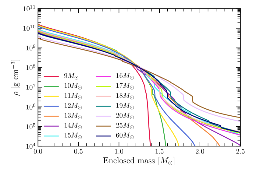
Figure 1: Density profiles for the progenitors considered in our study. We obtain successful explosions for both low-compactness stellar cores, such as those of the 9-M_⊙ and 10-M_⊙ progenitors, as well as for high-compactness stellar cores with sharp density drops at the Si/O interface, such as that of the 25-M_⊙ progenitor.

Progenitor	Envelope Binding Energy	Compactness
(M⊙)	($10^{51}$ ergs)	(calculated at 1.75 M⊙)
s9.0	0.002	$3.831\times{10^{-5}}$
s10.0	0.012	$2.165\times{10^{-4}}$
s11.0	0.025	$7.669\times{10^{-3}}$
s12.0	0.050	$2.215\times{10^{-2}}$
s13.0	0.072	$5.932\times{10^{-2}}$
s14.0	0.110	0.1243
s15.0	0.144	0.1674
s16.0	0.212	0.1546
s17.0	0.251	0.1644
s18.0	0.309	0.1715
s19.0	0.341	0.1783
s20.0	0.413	0.2615
s25.0	0.865	0.3010
s60.0	0.513	0.1753

Table 1: The binding energy (in units of $10^{51}$ ergs, one Bethe) of the stellar envelope exterior to the 20,000 km outer boundary of the computational domain and the so-called compactness of the progenitor, calculated at 1.75 M_⊙. The former is the energy penalty an explosion witnessed on the computational domain still has to pay to eject that outer envelope material and reach “infinity." The compactness is a crude, but ofttimes useful, metric of the shallowness of the mass density profile of the inner progenitor. It has been shown that while compactness is not a measure of explodability it is roughly correlated with the envelope binding energy (Burrows et al., 2018), a proposition this table supports.

The mass density profiles of massive stars were once thought to be roughly monotonic with ZAMS mass. This might have translated into a smooth dependence upon progenitor mass of the explosion characteristics, for a given metallicity. However, recent 1D studies (Sukhbold et al., 2016; Sukhbold et al., 2018; Woosley, 2019) have called this simple picture into question, with slight “chaos" resulting in a non-monotonic dependence on the shallowness of the mass density profile in the crucial inner core. Figure 1 depicts the mass density profiles for the initial models we employ for this study. In addition, Table 1 provides for our model suite the “compactness," a simple one-dimensional metric of shallowness (O’Connor & Ott, 2013). Compactness does affect the evolution of the infall accretion rate, and, hence, the neutrino luminosities and neutrino energies. Therefore, in the context of the neutrino-driven mechanism of explosion, it affects whether, when, and how a model explodes. However, we have found in recent studies in 2D (Burrows et al., 2018) and 3D (Burrows et al., 2019) that this naive picture is not complete and that explodability is not correlated with compactness in a simple way. With this paper, we expand this notion and find that the 13-, 14-, and 15-M_⊙ models (not only the 13-M_⊙ model studied in Burrows et al. 2019), fail to explode, when all the other models do. This makes more firm the preliminary conclusion in Burrows et al. (2019) that there may be a mass gap in explodability near the middle of the massive-star mass function. In fact, we now find, and demonstrate in this paper, that both low and high compactness models explode, with the high compactness models likely exploding the most energetically, albeit later. It was once thought that low compactness and a steep initial density profile were prerequisites for explodability. Our new results put this notion in doubt.

To add further complexity, recent 3D stellar evolution studies reveal mixing processes, gravity waves, and dynamics that the problematic mixing-length prescription for convection can not capture and, therefore, that the progenitor landscape is still not fully understood (Couch et al., 2015; Jones et al., 2016; Chatzopoulos et al., 2016; Müller et al., 2017; Müller et al., 2019; Jones et al., 2019; Yoshida et al., 2019). Moreover, the potential role of aspherical perturbations in the progenitor models in inaugurating and maintaining turbulent convection behind the stalled shock wave (Couch & Ott, 2015; Müller et al., 2017; Burrows et al., 2018; Vartanyan et al., 2018; Müller et al., 2019), shown to be important in igniting neutrino-driven explosions (Burrows et al., 1995), highlights the need to determine their magnitude and character. One-dimensional stellar-evolution calculations are clearly not adequate. Therefore, the reader should keep in mind the provisional character of current progenitor models employed by supernova theorists and the ongoing need for further improvement. Nevertheless, such is the span of the mass density profiles of the model continuum we incorporate in this study that though the derived mapping between ZAMS and outcome itself is probably provisional, the range of behaviors in this wide progenitor range from 9 M_⊙, through 25 M_⊙, to 60 M_⊙ is probably, in the main, captured.

In this paper, in addition to determining whether and when these models explode, we present the shock radius development, the integrated neutrino luminosities, the final masses of exploding models, the neutrino heating rates, the spherical-harmonic decompositions of the shock surface, the diagnostic explosion energy and its rate of climb, the ejecta masses, the ejecta electron-fraction (Y_e) distributions, and approximate maps of the putative ejecta ⁵⁶Ni distributions. In §2, we describe in detail the specifications of Fornax and the computational setup employed for this paper. In §3, we provide our results, including explosion properties, the integrated neutrino luminosities, the spherical-harmonic decompositions of the shock surface, the diagnostic explosion energy and its rate of climb, the neutrino heating rates, the final neutron-star masses of exploding models, the ejecta masses and the ejecta electron-fraction (Y_e) distributions, and approximate maps of the inferred ejecta ⁵⁶Ni distributions. In §4, we show how a model’s hydrodynamic behavior might depend upon resolution, the Horowitz many-body correction, and employing a monopole term in place of a multipole expansion to handle gravity. We summarize our general results and conclusions in §5.

2 Numerical Methods and Computational Setup

The numerical and physical details incorporated into the code Fornax have been published in numerous papers in recent years (Skinner et al., 2016; Burrows et al., 2018; Vartanyan et al., 2018; Burrows et al., 2019; Skinner et al., 2019). In particular, Skinner et al. (2019) provided a challenging set of hydrodynamic, radiation, and radiation-hydrodynamic tests and described the discritization, reconstruction, solver, algorithms, and implementation specifics of Fornax.

Most of the code is written in C, with only a few Fortran 95 routines for reading in microphysical data tables; we use an MPI/OpenMP hybrid paralelism model. Fornax employs spherical coordinates in one, two, and three spatial dimensions, solves the comoving-frame, multi-group, two-moment, velocity-dependent transport equations to O($v/c$), and uses the M1 tensor closure for the second and third moments of the radiation fields (Vaytet et al., 2011). We do not use the dimensional reduction simplification known as “ray-by-ray+" employed by most other groups, but follow the vector flux densities of the first-moment equations in 3D. The ray-by-ray+ approach, though it addresses the lateral advective transport of lepton number, has been shown to introduce artifacts in the results, particularly for 2D simulations (Skinner et al., 2016) and aspherical 3D simulations (Glas et al., 2019).

Three species of neutrino ($\nu_{e}$, $\bar{\nu}_{e}$, and “$\nu_{\mu}$" [$\nu_{\mu}$, $\bar{\nu}_{\mu}$, $\nu_{\tau}$, and $\bar{\nu}_{\tau}$ lumped together]) are followed using an explicit Godunov characteristic method applied to the radiation transport operators, but an implicit solver for the radiation source terms. In this way, the radiative transport and transfer are handled locally, without the need for a global solution on the entire mesh. This is also the recent approach taken by O’Connor & Couch (2018), Glas et al. (2019), and O’Connor & Couch (2018), though with some important differences. By addressing the transport operator with an explicit method, we significantly reduce the computational complexity and communication overhead of traditional multi-dimensional radiative transfer solutions by bypassing the need for global iterative solvers that have proven to be slow and/or problematic beyond $\sim$10,000 cores. Strong scaling of the transport solution in three dimensions using Fornax is excellent beyond 100,000 tasks on KNL and Cray architectures. The light-crossing time of a zone generally sets the timestep, but since the speed of light and the speed of sound in the inner core are not far apart in the core-collapse problem after bounce, this numerical stability constraint on the timestep is similar to the CFL constraint of the explicit hydrodynamics. Radiation quantities are reconstructed with linear profiles and the calculated edge states are used to determine fluxes via an HLLE solver. In the non-hyperbolic regime, the HLLE fluxes are corrected to reduce numerical diffusion (O’Connor & Ott, 2013). The momentum and energy transfer between the radiation and the gas are operator-split and addressed implicitly.

The hydrodynamics in Fornax is based on a directionally unsplit Godunov-type finite-volume method. Fluxes at cell faces are computed with the fast and accurate HLLC approximate Riemann solver based on left and right states reconstructed from the underlying volume-averaged states. The reconstruction is accomplished via a novel algorithm we developed specifically for Fornax that uses moments of the coordinates within each cell and the volume-averaged states to reconstruct TVD-limited parabolic profiles, while requiring one less “ghost cell" than the standard PPM approach. The profiles always respect the cells’ volume averages and, in smooth parts of the solution away from extrema, yield third-order accurate states on the faces. To eliminate the carbuncle and related phenomenon (Hanawa et al., 2008), Fornax specifically detects strong, grid-aligned shocks and employs in neighboring cells HLLE, rather than HLLC, fluxes that introduce a small amount of smoothing in the transverse direction. Currently, we do not include the effects of nuclear burning. Given the ejecta masses we obtain (§3.6), we expect this usually to amount to no more than a $\sim$10% effect on the explosion energies (however, see §3.2), but this remains to be seen (Yamamoto et al., 2013).

Without gravity, the coupled set of radiation/hydrodynamic equations conserves energy and momentum to machine accuracy. Total lepton number is conserved by construction. With gravity, energy conservation is excellent before and after core bounce (Skinner et al., 2019). However, as with all other supernova codes, at bounce the total energy as defined in integral form glitches by $\geq 10^{49}$ ergs. This is due to the fact that the gravitational terms are handled in the momentum and energy equations as source terms and are not in conservative divergence form.

The code is written in a covariant/coordinate-independent fashion, with generalized connection coefficients, and so can employ any coordinate mapping. This facilitates the use of any logically-Cartesian coordinate system and, if necessary, the artful distribution of zones. In the interior, to circumvent Courant limits due to converging angular zones, the code can deresolve in both angles ($\theta$ and $\phi$) independently with decreasing radius, conserving hydrodynamic and radiative fluxes in a manner similar to the method employed in AMR codes at refinement boundaries. The use of such a “dendritic grid," or “static-mesh refinement," allows us to avoid angular Courant limits at the center, while maintaining accuracy and enabling us to employ the useful spherical coordinate system natural for the supernova problem.

Importantly, the overheads for Christoffel symbol calculations are minimal, since the code uses static refinement, and, hence, the terms are calculated only once (in the beginning). Therefore, the overhead associated with the covariant formulation is almost nonexistent. In the context of a multi-species, multi-group, neutrino radiation hydrodynamics calculation, the additional memory footprint is small (note that the radiation requires hundreds of variables to be stored per zone). In terms of FLOPs, the additional costs are associated with occasionally transforming between contravariant and covariant quantities and in the evaluation of the geometric source terms. Again, in the context of a radiation/hydrodynamics calculation, the additional expense is extremely small.

Gravity can be handled in 2D and 3D with a multipole solver (Müller & Steinmetz, 1995), where we would generally set the maximum spherical harmonic order necessary equal to twelve. For these calculations however, to gain a bit of speed, we use the monopole only (see §4). In all implementations of gravity, the monopole gravitational term is altered to approximately accommodate general-relativistic gravity (Marek et al., 2006) and we employ the metric terms, $g_{rr}$ and $g_{tt}$, derived from this potential in the neutrino transport equations to incorporate general relativistic redshift effects (in the manner of Rampp & Janka (2002); see also Burrows et al. (2018)). We use for this extensive suite of simulations the SFHo EOS of Steiner et al. (2013). This EOS is one of those still consistent with known laboratory nuclear physics constraints (Tews et al., 2017). However, the study of the EOS dependence of core-collapse theory is one of the important topics for future research (Souza et al., 2009; Hempel et al., 2012; Couch, 2013; Suwa et al., 2013; Steiner et al., 2013; da Silva Schneider et al., 2017; Nagakura et al., 2018; Schneider et al., 2019).

The neutrino-matter interaction cross sections and rates are taken from Burrows et al. (2006) and we use detailed balance to derive emissivities from absorption rates. Many-body corrections to the axial-vector part of the neutrino-nucleon scattering rate are taken from Horowitz et al. (2017). All our default simulations incorporated this correction. We note that such corrections for both neutral-current scattering and charged-current absorption are still in play and have been shown to be potentially important (Burrows et al., 2018; Burrows & Sawyer, 1998). Weak magnetism and recoil corrections to scattering and absorption rates off nucleons à la Horowitz (2002) are employed. Coherent Freedman scattering off nuclei is corrected using lepton screening and form-factor terms described in Burrows et al. (2006). Nucleon-nucleon bremmstrahlung is handled using the rates found in Thompson et al. (2000) and our approach to $e^{+}/e^{-}$ annihilation into neutrino pairs is found in both Thompson et al. (2000) and Burrows et al. (2006). Inelastic scattering of neutrinos and anti-neutrinos off electrons and free nucleons is addressed using the prescriptions described in Thompson et al. (2003), with more details of its implementation to be found in Burrows & Thompson (2004). Our approach to electron capture on heavy nuclei, most important on infall, is taken from Juodagalvis et al. (2010).

To summarize, the advantages of Fornax are: 1) it does not employ the simplifying “ray-by-ray+" approximation used by many others (Tamborra et al., 2014; Lentz et al., 2015; Melson et al., 2015; Müller, 2015; Takiwaki et al., 2016; Müller et al., 2017; Summa et al., 2018) that suppresses the important lateral transport (Skinner et al., 2016); 2) it handles the spatial transport operator explicitly, thereby avoiding problematic global iterative solves; 3) the source terms are still handled implicitly, including inelastic energy redistribution, ensuring stability and speed; 4) we use static-mesh-refinement in the inner core and along the polar axis to thwart the significant Courant timestep hit in the angular directions that would otherwise obtain there when using spherical coordinates; and 5) all important physical effects (except neutrino oscillations) are handled at some reasonable level of approximation. In short, all the necessary physical realism is included. The result is a code that is $\sim$5 times faster than previous implementations, and this speedup is what enables the significant increase in simulation cadence represented by this paper. Drawbacks of the current implementation of Fornax are that it incorporates approximate general-relativistic gravity and does not perform full multi-angle transport. Though Fornax does follow the multi-group vector fluxes, it is currently too expensive to attempt to calculate the full angular specific-intensity distributions in 3D for a simulation of reasonable physical duration (Nagakura et al., 2014; Nagakura et al., 2017; Nagakura et al., 2019).

In keeping with the philosophy behind this comprehensive 3D study spanning such a unprecedentedly wide progenitor mass range, we start our calculations with a uniform set of progenitors taken from Sukhbold et al. (2016). The only exception is the 25-M_⊙ model, taken from Sukhbold et al. (2018). This 3D full-physics model set includes 9-, 10-, 11-, 12-, 13-, 14-, 15-, 16-, 17-, 18-, 19-, 20-, 25-, and 60-M_⊙ massive-star progenitors. In addition, we explore for a subset of progenitors the multipole/monopole, Horowitz/no-Horowitz, low versus high angular resolution differences for a small subset of progenitors, namely the 19-M_⊙ and 11-M_⊙ models. We explored in a previous paper (Nagakura et al., 2019) other aspects of the same resolution study. In toto, this comprises nineteen 3D simulations with what is thought to be the necessary physical realism.

Unless otherwise indicated, our default spatial resolution is 678$\times$128$\times$256 (r$\times\theta\times\phi$), we use 12 energy groups, and the outer radius is at 20,000 kilometers (km). The radial zone width from the center out to $\sim$20 km is 0.5 km, after which the zone width grows logarithmically to this outer boundary. The energy groups are logarithmically distributed from 1 MeV to 300 MeV (for $\nu_{e}$) or 100 MeV (for all other species). To seed instabilities, very modest initial perturbations to the velocity field of amplitude 100 km s^-1 and with $\ell=10$, $m=1$, and $n=4$, using the prescription of Müller & Janka (2015), were imposed 10 milliseconds (ms) after bounce to the 3D model that was mapped from the 1D model followed to collapse. This is to be compared to the pre-explosion speeds in front of the bounce shock of $\sim$50,000 km s^-1 and the immediate post-bounce speeds from $\sim$8000 km s^-1 to $\sim$4000 km s^-1. It is expected that these perturbations will grow on infall (Lai & Goldreich, 2000; Takahashi & Yamada, 2014), but not achieve comparable speeds. All models were non-rotating. We have attempted to standardize all model runs to ensure our model-to-model comparisons are as direct as possible. In this way, one can hope to better ascertain true systematic differences in the context of state-of-the-art 3D simulations over this wide progenitor panorama.

We emphasize that all our 3D models are calculated using exactly the same specifications and setup, including our admittedly-crude method of initial model perturbation. This is to enable direct comparisons and, thereby, to extract systematic variations along the progenitor continuum. It may be that models for which we don’t witness explosions (and vice versa) might explode with rotation, updated physics, higher resolution, or an improved code, etc. However, we assert that the relative tendency to explode, or not to explode, is captured by our study and will serve as an important theoretical context going forward.

3 Results

3.1 Overview

Figure 2: Average shock radii. Our models span a wide range in terms of explosion delay times with shock revival occurring from ${\sim}0.1$ to ${\sim}0.5$ seconds after bounce. Among the progenitors we consider, the 13-M_⊙, 14-M_⊙ and 15-M_⊙ models fail to explode within the timeframe we simulate.

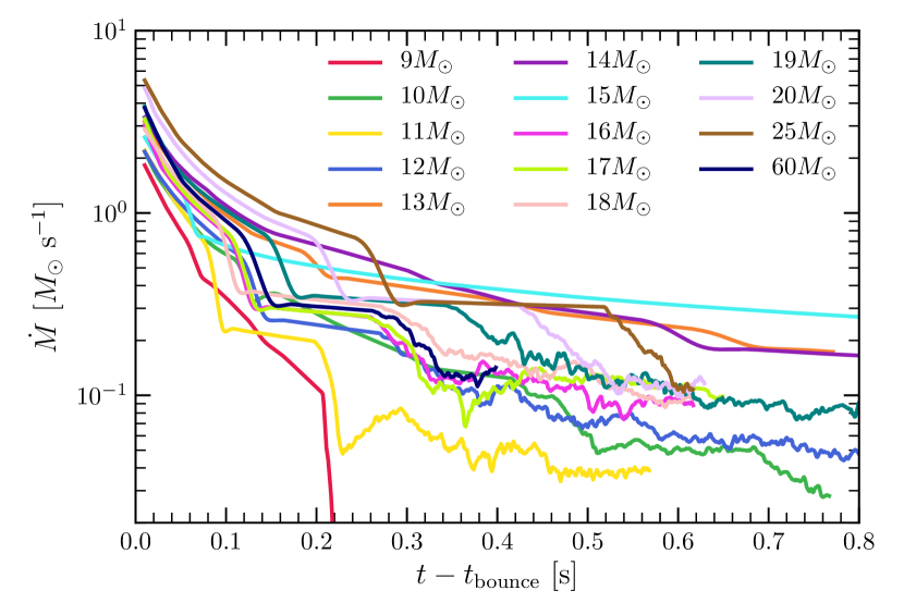
Figure 3: Mass accretion rate at 500 km. All exploding models display a sharp drop in the accretion rate corresponding to the infall of the Si/O interface. All models, with the exception of the 9-$M_{\odot}$ progenitor, show an overall positive net accretion rate onto the inner core even after explosion sets in.

At this stage in the theoretical development of progenitor models, it should not be assumed that the mapping between mass and profile is accurately known. There is still much churn in that complicated field, and the effects of multi-dimensional stellar evolution (Couch et al., 2015; Jones et al., 2016; Chatzopoulos et al., 2016; Müller et al., 2017; Müller et al., 2019; Jones et al., 2019; Yoshida et al., 2019) and binarity (Müller et al., 2019), to name only two, have not yet been fully assimilated. However, it is reasonable to suggest that the range of possible structures is well-captured by the range depicted in Figure 1. It is in this spirit that we present our 3D explosion results and suggest that the general range of outcomes has been approximately corralled.

Figure 1 depicts the mass density profiles of the suite of models upon which we focus in this paper. The range of model slopes exterior to $\sim$1.2 M_⊙ is quite wide and covers most of the model space historically found in the literature. The lowest mass representative, the 9-M_⊙ progenitor, boasts the steepest profile and the 25-M_⊙ progenitor the shallowest, and any measure of average declivity would be a monotonic function of ZAMS mass. However, as the calculated compactness given in Table 1 demonstrates, the models are not perfectly nested monotonically, and this is thought to reflect real physical effects (Woosley & Heger, 2007; Sukhbold et al., 2016; Sukhbold et al., 2018). Moreover, due to significant mass loss, the 60-M_⊙ of Sukhbold et al. (2016) we employ in this paper resides in the middle of the pack. For all the models, the compactness and shallowness are inversely related to the central density, which helps determine the time to bounce. It should be noticed that most of the models have pronounced density cliffs at the silicon/oxygen interface, and it has been shown that the accretion of such features can itself jump a model into explosion (Vartanyan et al., 2018; Burrows et al., 2018; Burrows et al., 2019). However, not all progenitors share this feature, with the 13-, 14-, and 15-M_⊙ models evincing some of the most modest jumps of $\sim$1.2 - 1.4. As Figure 2 of the post-bounce evolution of the mean shock radius demonstrates, these are the models that do not explode, and this is one reason. All our other models explode, with the post-bounce explosion times generally shorter for the lower-mass progenitors and longer for the higher-mass progenitors. Most of these exploding models have mass density jumps at this interface of $\sim$2.0-2.3. Here, we define the time of explosion rather loosely as the approximate time the mean shock radius experiences an upward inflexion and is seen to continue its climb. In fact, the 19-, 20-, and 25-M_⊙ stars explode later than most, and the 9- and 11-M_⊙ models the earliest, with the 10-M_⊙ model a bit sluggish, perhaps due to the less pronounced silicon/oxygen ledge and its (seemingly anomalous) shallower density profile. However, the general separation of the early-exploding lower-mass branch from the later exploding higher-mass branch seems to hold. The delay of the higher-mass models seems connected with the larger early mass accretion rate (Figure 3) and higher associated ram pressure. However, when these models do explode they do so more energetically $-$ the higher accretion rates are maintained to translate into higher driving neutrino luminosities (Figure 4, left) and RMS neutrino energies (Figure 4, right) absorbed on a consequently thicker column of mass in the gain region, resulting in a higher neutrino power deposition (Figure 5). As we discuss in §3.2, this results in a higher accumulation rate of net explosion energy, and likely into higher asymptotic explosion energies. Nevertheless, we still find that there are models, currently in the middle of the progenitor continuum, that do not explode, but are bracketed in compactness and other general parameters by those that do. This reiterates the strong conclusion that low compactness is not a necessary nor sufficient condition for explodability (Burrows et al., 2018).

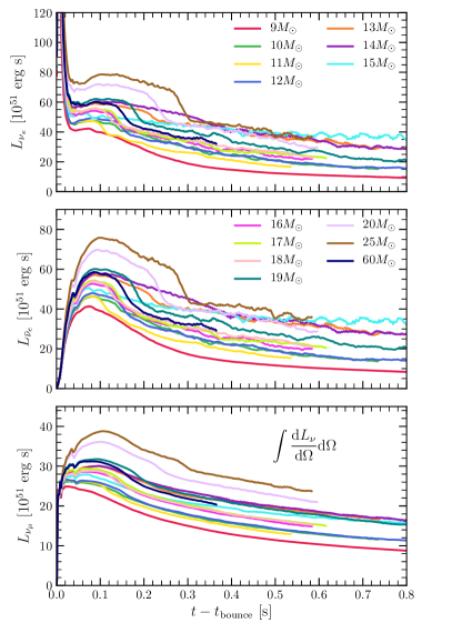
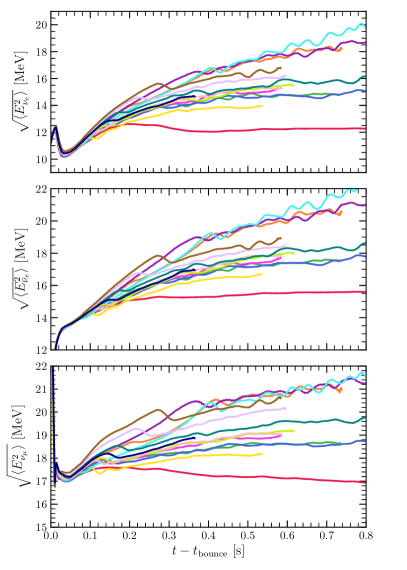
Figure 4: Neutrino luminosities (left panel) and rms energies (right panel) measured at 10,000 km. There is significant spread between the different models. The exploding models, with the exception of the 9-M_⊙ progenitor, show drops in the electron-type neutrino luminosities at the time of the accretion of the Si/O interface, which coincides with the explosion time. The explosion time is also imprinted in the neutrino rms energies, which exhibit a similar drop.

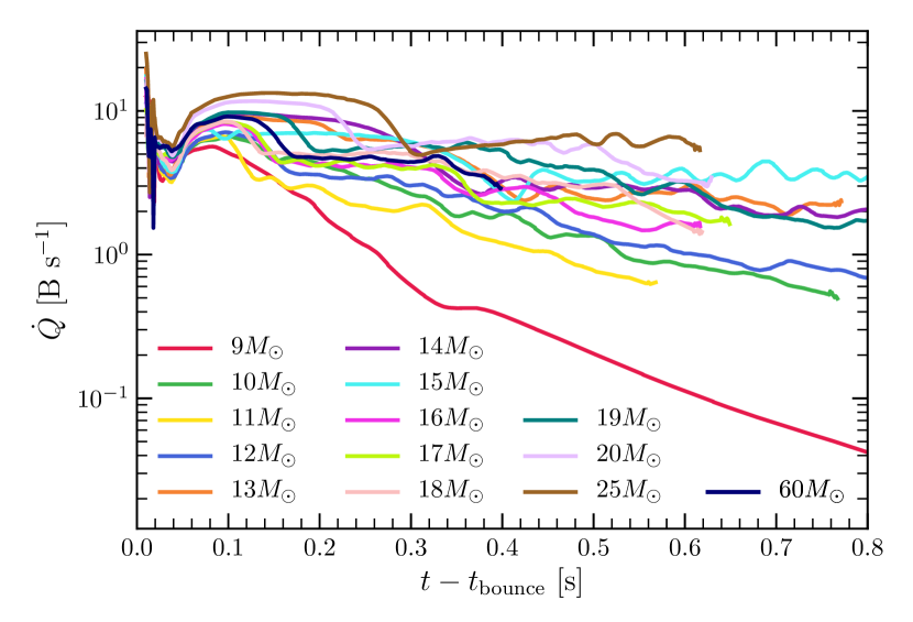
Figure 5: Net neutrino energy deposition rate. More compact progenitors typically show higher neutrino luminosities and higher net heating rates. With the exception of the 9-M_⊙ progenitor, strong heating is maintained for the entire duration of our simulations.

Figure 3 renders the evolution of the integrated mass accretion rate ($\dot{M}$, inward) through a radius of 500 km as a function of time after bounce. $\dot{M}$ follows the corresponding mass density profile (Figure 1) closely, with the effects of the accretion of the silicon/oxygen interface clearly shown. The post-bounce time of the accretion of this interface is correlated for many models with the onset time of explosion (modulo the accretion time from 500 km to the shock). $\dot{M}$ for the 9-M_⊙ model drops precipitously, and accretion effectively ceases around $\sim$0.2 seconds. Not unexpectedly, $\dot{M}$ for the non-exploding models (13-, 14-, and 15-M_⊙) continues and eventually (after $\sim$0.6 seconds) supersedes that of any exploding model. However, apart from the 9-M_⊙ model, even for the exploding models accretion continues for quite some time. This is due to the fact that in 3D there simultaneously can be accretion in one direction, while the star explodes in another. This feature enables accretion to maintain the driving neutrino luminosities beyond the onset of explosion at a higher level than would be possible with core neutrino diffusion alone, and is clearly pronounced for the 25-M_⊙ model. For the exploding models, we note that with time $\dot{M}$ at 500 km begins very weakly fluctuating behavior on timescales of $\sim$10 milliseconds. This is due to the summed effect of the clumpiness and swirling behavior of the ejected material at a radius of 500 km after the exploding turbulent shock has reached and passed it with the dominant accretion component associated with the material that continues to infall despite explosion at other angles (Müller et al., 2017; Vartanyan et al., 2019).

The post-bounce evolutions of the angle-integrated neutrino luminosities and RMS neutrino energies are given in Figure 4. The hierarchy of values expected from the systematics with progenitor with $\dot{M}$ depicted in Figure 3 is continued in these plots. The lower-mass progenitors generally achieve lower luminosities, with the plateaus/peaks in the $\nu_{e}$ (post-breakout) and $\bar{\nu}_{e}$ luminosities ranging by a factor of $\sim$2 and in the $\nu_{\mu}$ luminosities by $\sim$60%. There is a similar systematic behavior for the mean and RMS neutrino energies, with higher neutrino energies generally for the more massive exploding progenitors. Since the neutrino energy deposition rate in the gain region behind the shock goes as the absorption cross section, which is quadratic in the RMS energy, the more massive models experience the double effect of both high luminosity and high neutrino energy. This result underpins the more rapid rise in explosion energy shown in Figure 6 for the 20- and 25-M_⊙ models. However, as Figure 4 indicates, at later times the neutrino energies for the non-exploding models continue to rise to achieve the highest values. This is also the case for their late-time luminosities. Therefore, despite the high values for the non-exploding models of the product of the luminosity and square of the RMS energy, they still need to explode for them to take advantage of this high product.

We note that the neutrino energies reached by all models are still significantly lower than those published by Wilson in his early, pioneering studies (Bethe & Wilson, 1985; Mayle et al., 1987). This is due to subsequent improvements in the neutrino-matter interaction rates and is reflected broadly in the modern literature (Bruenn et al., 2016; Janka, 2017; O’Connor et al., 2018; Glas et al., 2019).

The heating rates (minus those due to inelastic scattering) in the gain region behind the shock are portrayed in Figure 5 and recapitulate the trends seen in Figures 3 and 4. The high deposition rates of a few to $\sim$10 Bethes (10⁵¹ ergs) per second should not lead one to infer that an asymptotic explosion energy of a Bethe is quickly achieved. Before explosion, this energy is completely reradiated and after the onset of explosion much of this power goes into lifting the ejecta out of a deep potential well.

Table 2 provides the mean shock radius and mean shock speed at the end of each of our baseline simulations. In general, soon after the shock is launched its mean speed stays roughly constant. The 9-M_⊙ model proceeded the furthest after bounce, at which point its explosion shock achieved a mean radius of $\sim$12,400 km and a mean shock speed of $\sim$1.6$\times{10}^{9}$ cm s^-1. The other exploding models achieved mean speeds of $\sim$5$-$8$\times{10}^{9}$ cm s^-1, while, as Table 2 clearly indicates, the 13-, 14-, and 15-M_⊙ do not explode.

3.2 Explosion Energies

Though many of our models were carried out to post-bounce times that would be considered late in the context of most other published 3D models, we find that the majority of our simulations still need to be carried out even further to asymptote to their final explosion energies. In a resource-constrained computational environment, deciding to be wider in progenitor space naturally translates into being shorter in mean duration. Nevertheless, ours is still by far the largest number of total physical-seconds explored in 3D. As Figure 6 shows, though the 11- and 12-M_⊙ simulations seem, by the curvature of their energy curves, to have reached within greater than $\sim$50% of their asymptotic explosion energies at simulation end, the only model in our set to actually asymptote to its final explosion energy is the 9-M_⊙ model (Burrows et al., 2019). It achieves an explosion energy of $\sim$10⁵⁰ ergs ($\sim$0.1 Bethe) after $\sim$0.5 seconds and was continued to $\sim$1.0 seconds.

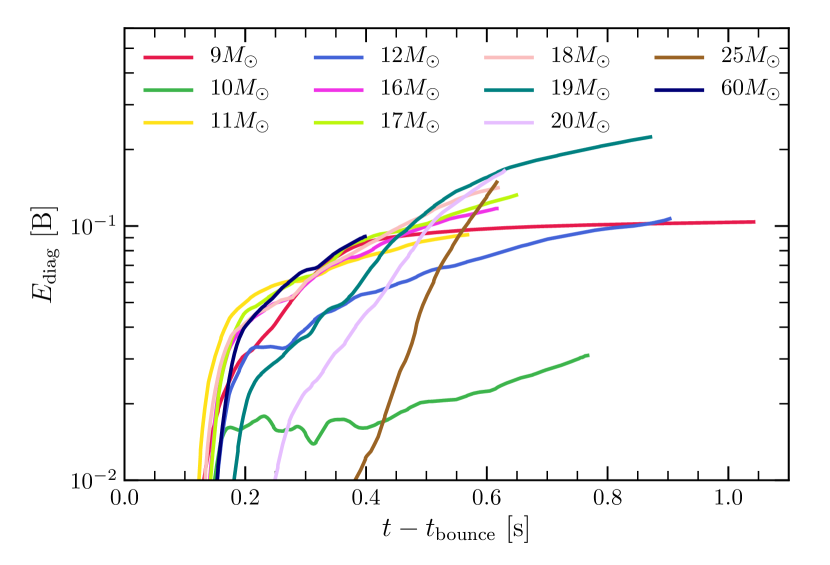
Figure 6: Diagnostic explosion energies. With the exception of the 9-M_⊙ progenitor, the explosion energies have not yet reached their asymptotic value. However, most of the models appear to be approaching diagnostic explosion energies near a $\mathrm{few}\times 10^{50}\ {\rm erg}$, except for the more massive models which are poised to achieve at later times even higher explosion energies. The total “diagnostic" supernova explosion energy is the sum of the internal thermal, kinetic, and gravitational energies of the ejecta, defined as the matter with positive Bernoulli integral. The gravitational term is the largest and much of the deposited neutrino power goes into work against it. We include in the diagnostic energy the “reassociation energy" of the debris into nuclei and the gravitational binding energy of the matter exterior to the explosion shock, but interior to the 20,000-km boundary. Note that the total diagnostic energy must still be corrected for the binding energy exterior to the outer computational boundary, provided in Table 1, to obtain the total explosion energy. This correction is small, except for the more massive models, where it can approach one Bethe.

Importantly, the higher-mass progenitors explode late (Figure 2), but, as stated in §3.1, accumulate total energy at a more rapid rate (Figure 6). For the 25-M_⊙ model, that rate is $\sim$1 Bethe per second and for the 20-M_⊙ model it is only a bit less, implying that, carried for another few seconds, these models would achieve what are considered to be “canonical" supernova energies of one Bethe or more. A caveat is that the total binding energy of the mantle exterior to our computational boundary at 20,000 km must be paid. As Table 1 indicates, though this number is quite small for the low-mass progenitors, it is approaching one Bethe for the 25-M_⊙ star, necessitating a longer energy ramp at the rate witnessed in Figure 6 to achieve a kinetic energy at infinity of order one Bethe. This longer time for the more massive stars is in keeping with the results of Müller (2015), who concluded the same using a simpler computational infrastructure. Hence, our results suggest that the more massive models that explode a bit later, likely ramp up more quickly to larger explosion energies after a longer evolution. For some massive models, perhaps the 25-M_⊙ model, the mantle binding energy penalty may be too high and a black hole may result. We note that since we have neglected nuclear burning, it is for the 25-M_⊙ model that this neglect may be most relevant. As we see in §3.6, the amount of core material ejecta for this model is large and a fraction of this mass (to be determined) may burn to boost this explosion even further. In this context it should be remembered that the burning of one solar mass of oxygen yields approximately a Bethe of energy.

The lower-mass progenitors explode, when they do, earlier after bounce, but achieve lower asymptotic explosion energies. This is the systematics in explosion energy with progenitor structure/mass that we infer from the results of this 3D progenitor model set. Importantly, this is also consistent with what is emerging from the progenitor-mass/explosion-energy correlation inferred in recent analyses of Type IIp light curves(Morozova et al., 2018; Martinez & Bersten, 2019; Eldridge et al., 2019; Poznanski, 2013). Clearly, future 3D simulations should push to longer post-bounce physical times. Moreover, the chaos in the convective turbulence will naturally introduce a degree of stochasticity in the outcomes and their parameters, including explosion energy. Therefore, determining the distribution functions in these observables, even for a given progenitor, will be an interesting long-term challenge for theory.

Progenitor	t(final)	Shock Radius	Shock Speed
(M⊙)	(seconds)	(1000 km)	(1000 km s-1)
s9.0	1.042	12.419	16.287
s10.0	0.767	1.963	6.647
s11.0	0.568	2.754	7.996
s12.0	0.903	4.088	6.944
s13.0	0.771	0.090	0.078
s14.0	0.994	0.077	0.044
s15.0	0.994	0.069	0.072
s16.0	0.617	2.265	6.717
s17.0	0.649	2.527	6.621
s18.0	0.619	2.122	7.870
s19.0	0.871	3.879	7.848
s20.0	0.629	1.415	7.330
s25.0	0.616	0.735	6.594
s60.0	0.398	0.808	5.233

Table 2: A table of the mean shock radius and mean shock speed at the end of each baseline 3D simulation. The simulation end time is given in seconds, the mean shock radius is given in units of 1000 km, and the mean shock speed is given in units of 1000 km s^-1. Note that the non-exploding models (13-, 14-, and 15-M_⊙) have correspondingly low values for both quantities.

Progenitor	t(final)	Baryon Mass	Grav. Mass
(M⊙)	(seconds)	(M⊙)	(M⊙)
s9.0	1.042	1.342	1.233
s10.0	0.767	1.495	1.358
s11.0	0.568	1.444	1.317
s12.0	0.903	1.517	1.377
s13.0	0.771	1.769	1.577
s14.0	0.994	1.824	1.619
s15.0	0.994	1.774	1.580
s16.0	0.617	1.585	1.431
s17.0	0.649	1.615	1.455
s18.0	0.619	1.606	1.448
s19.0	0.871	1.757	1.567
s20.0	0.629	1.887	1.667
s25.0	0.616	1.993	1.747
s60.0	0.398	1.647	1.481

Table 3: At the final time after bounce for each simulation (in seconds), the baryonic mass of the PNS (in M_⊙) and the gravitational mass of the residual neutron star (in M_⊙) for all the models of this study (except the extra 3D models associated with the sensitivity study of §4). All models, except the 13-, 14-, and 15-M_⊙ models, explode.

3.3 Proto-neutron Star Masses

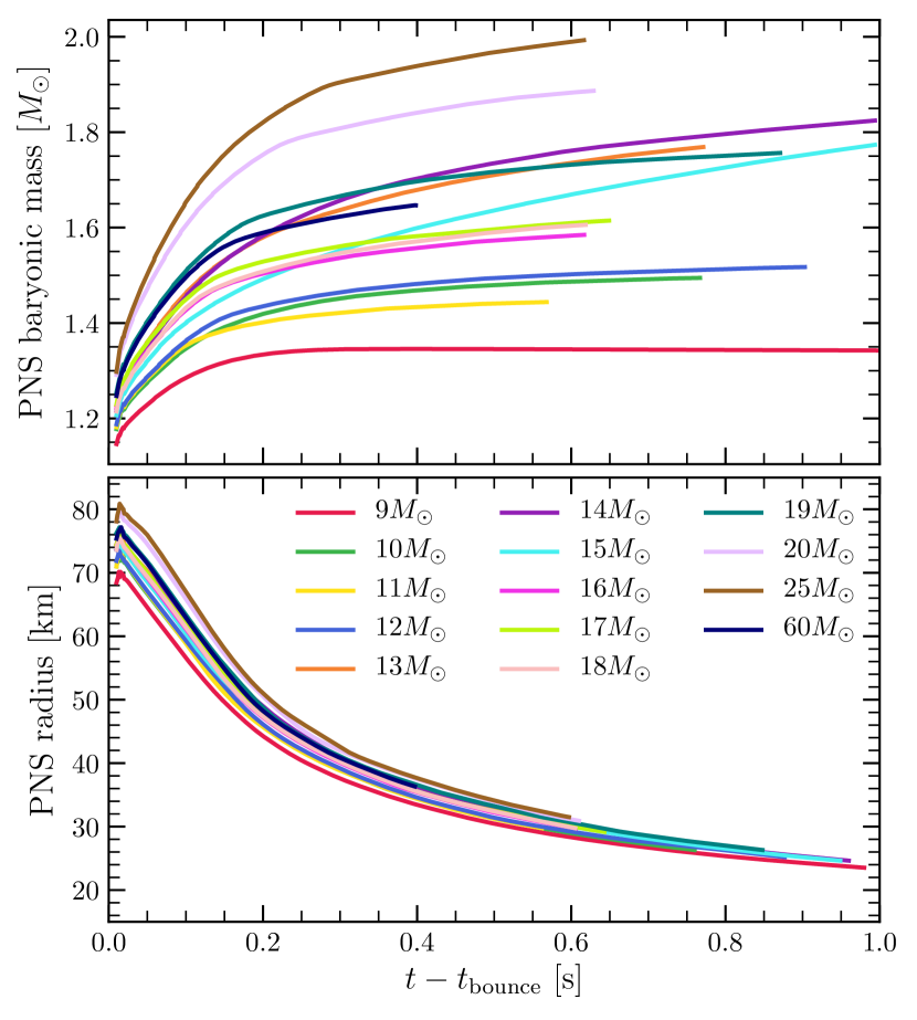
Figure 7: PNS baryonic masses (in M_⊙) (upper panel) and radii (in km) (lower panel). For most of the models the growth rate of the PNS has dropped substantially by the time we terminate our simulations. The PNS of the 25-M_⊙ progenitor, which explodes very energetically ${\sim}0.5$ seconds after bounce, is still growing rapidly at the end of the simulation.

Figure 7 shows the baryon mass accumulated within an isodensity surface of mass density 10¹¹ g cm^-3 for all the simulations of this investigation. This PNS mass ranges from a low of $\sim$1.3 M_⊙ for the 9-M_⊙ model to a high near $\sim$2.0 M_⊙ for the 25-M_⊙ progenitor. In Table 3, we tabulate the baryon and gravitational PNS masses at the end of each simulation. The latter is the gravitational mass for the cold neutron star in beta equilibrium, using the SFHo EOS. Except for the 9-M_⊙ simulation, for which the PNS mass has asymptoted, the PNS masses for the other models are still growing at a rate bounded by $\sim$5% per second at the termination of each run. While the PNS radius (defined as the $10^{11}$ g cm^-3 radius) for all models varies from one model to the next by no more than $\sim$15%, the gravitational mass varies by $\sim$40% from 1.233 to 1.747 M_⊙, a range in keeping with general expectations for neutron stars in the galaxy (Lattimer & Prakash, 2007). However, it does not extend to the highest values measured to date ($\sim$2.1 M_⊙, Antoniadis et al. (2013); $\sim$1.97 M_⊙, Demorest et al. (2010); $\sim$2.14 M_⊙, Cromartie et al. (2019)). Nevertheless, we see a clear trend among the exploding models from low neutron star masses for low-mass progenitors to higher mass neutron stars for the high-mass progenitors, with the 10-M_⊙ out of order (as discussed). Given the non-monotonicity of the initial mass-density profiles (Figure 1) with progenitor, we would not expect a monotonic correspondence between progenitor mass and residual PNS gravitational mass. Again, the non-exploding models in the middle of the compactness continuum are “out of sequence." Of course, if they never explode in the first seconds after bounce, they should birth black holes.

The PNS radii depicted in Figure 7 achieve values of only $\sim$25 km by the end of the simulations. This is not the standard 10-12 km because the PNS is still lepton-rich and hot. It will require many more seconds to one minute to cool and deleptonize into the “cold, catylyzed" state of a galactic neutron star (Burrows & Lattimer, 1986).

3.4 Explosion Morphology

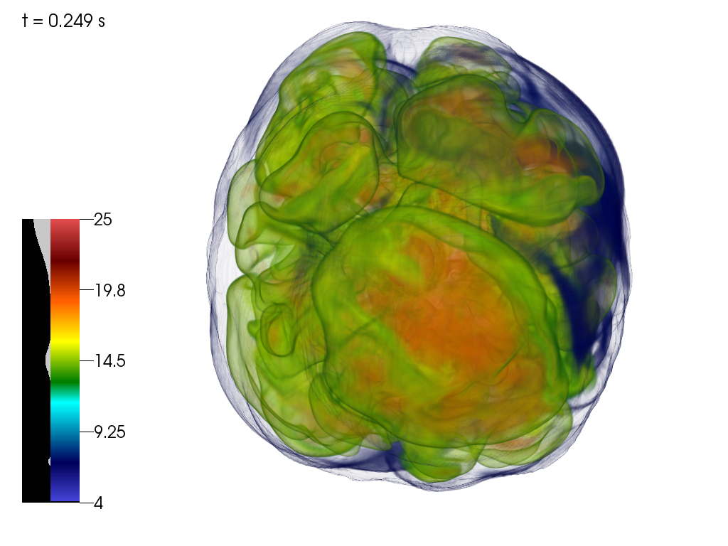
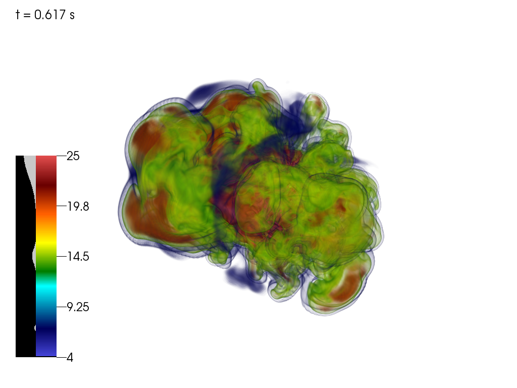
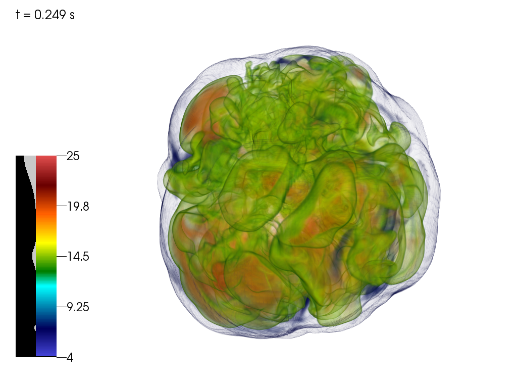
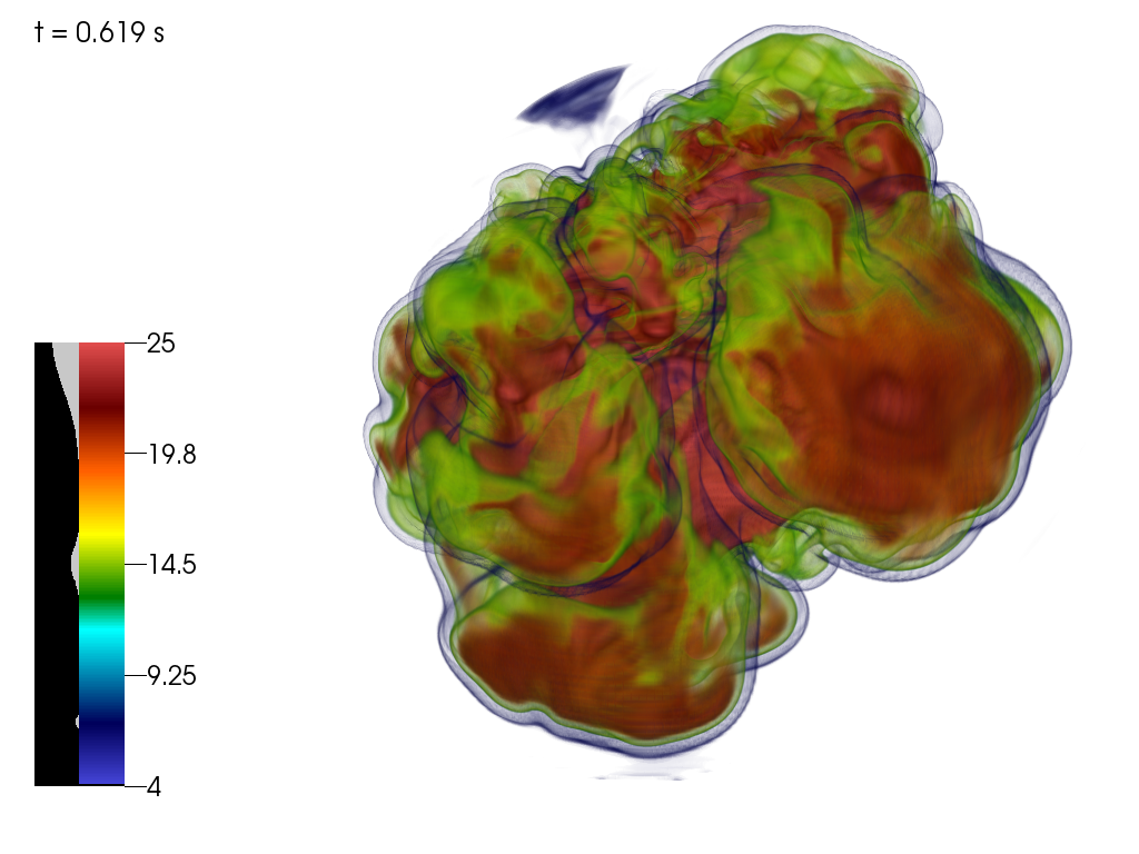
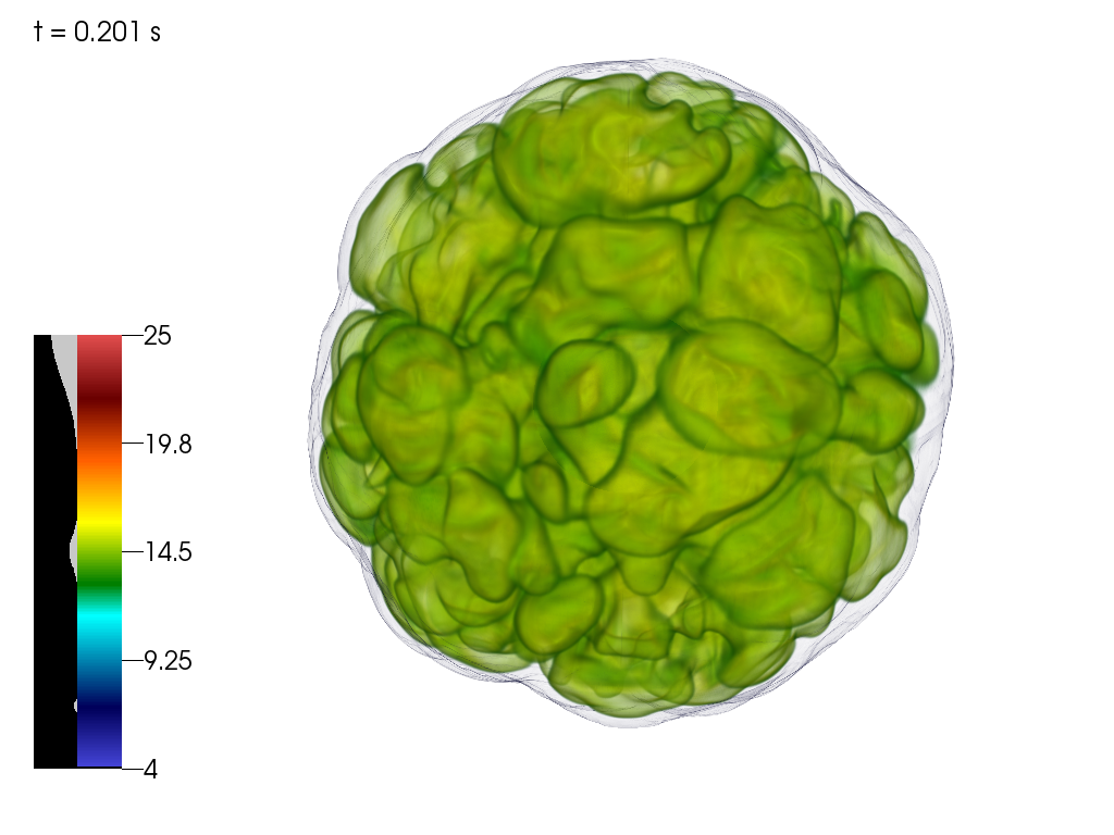
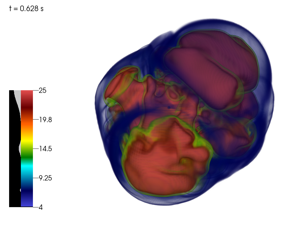
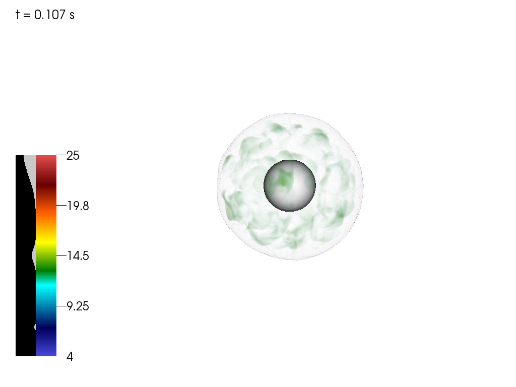
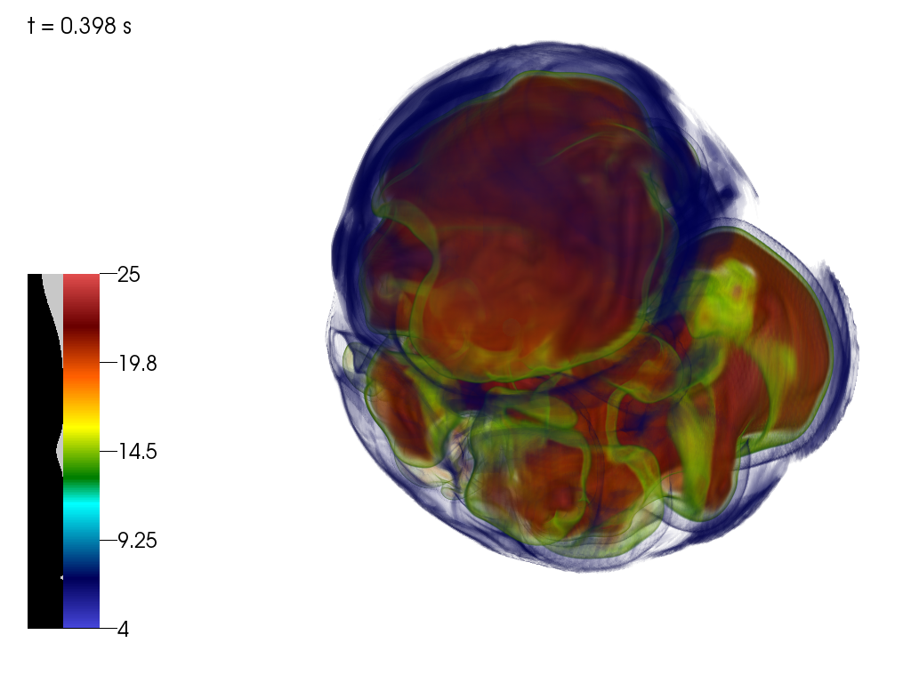
Figure 8: Volume renderings at two different times of four representative 3D models that explode. The 16-, 18-, 20-, and 60-M_⊙ models are portrayed from top to bottom. For these 16-, 18-, 20-, and 60-M_⊙ models, the times for the stills on the left 250, 250, 200, and 100 ms after bounce, respectively, and on the right are 637, 639, 651, and 400 ms after bounce, respectively. The blue veil on each plot roughly traces the position of the shock. Also shown are the entropy (per baryon per Boltzmann’s constant) colormaps for each model and time. Note the transition to redder colors at the later times, indicative of the higher entropies generated through ongoing neutrino heating. The physical scales are (left plot, right plot) = ($\pm$320 km/$\pm$2240 km; $\pm$320 km/$\pm$2000 km; $\pm$160 km/$\pm$1600 km; and $\pm$160 km/$\pm$960 km), respectively.

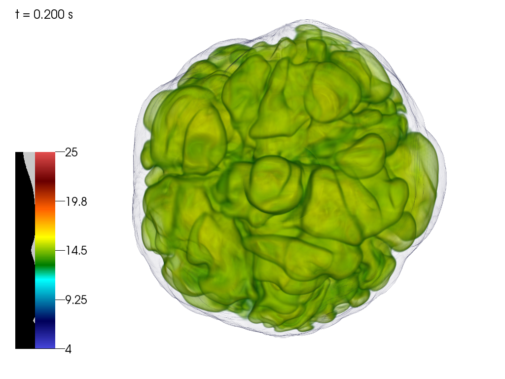
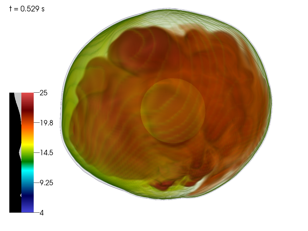
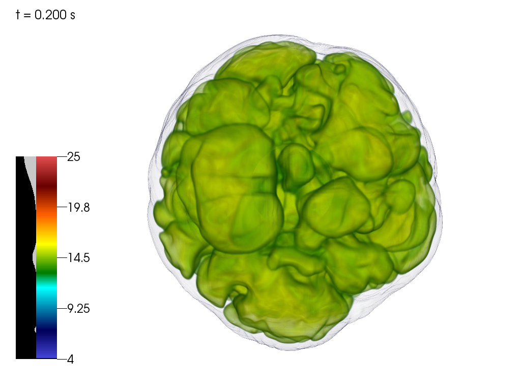
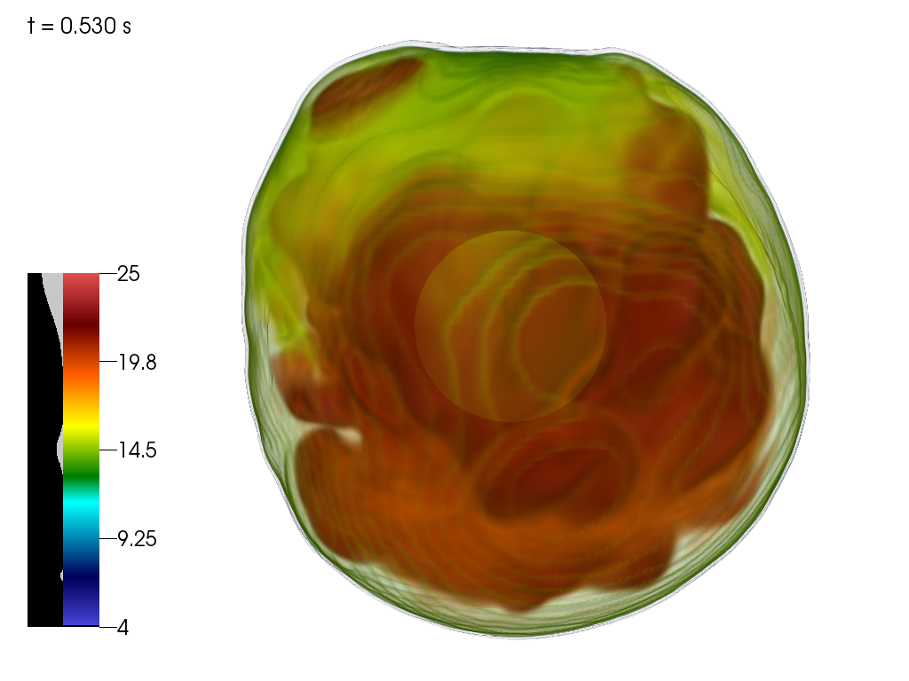
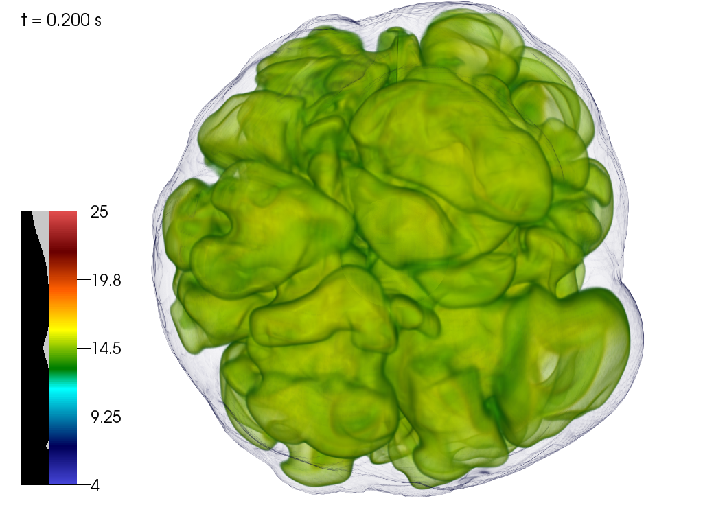
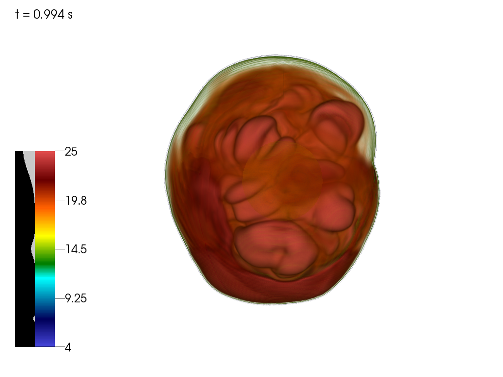
Figure 9: Same as Figure 8, but for the three default 3D models that do not explode. The 13-, 14-, and 15-M_⊙ models are portrayed from top to bottom. For these 13-, 14-, and 15-M_⊙ models, the times for all the stills on the left are all 200 ms after bounce, and on the right are 550, 550, and 1048 ms after bounce, respectively. Despite the transition to redder colors at the later times, indicative of the higher entropies generated through ongoing neutrino heating, these models do not explode. Note the presence of the spheres in the centers on the right. This is the proto-neutron star (PNS), here given as a 10¹¹ gm cm^-3 mass-density isosurface. The physical scales are $\pm$160 km/$\pm$80 km (left/right) for all three model plots. See text for a discussion.

Figure 8 summarizes the evolution before and after explosion of a subset of our exploding models. At early times before or near the onset of explosion the rough shape of the shock is spherical, with significant bubble structures and a range of scales. The green color that dominates on the left (early phase) indicates modest entropies generated due to ongoing neutrino heating (Figure 5). With time and as the explosion progresses, these colors turn progressively more red as the entropies rise and higher-entropy bubbles drive the explosion. A feature of many of our exploding models is the slight pinching near the middle of the exploding structures (Vartanyan et al., 2019; Burrows et al., 2019) seen on the right panels of Figure 8. This is due to accretion of matter in a belt while the rest of the mantle is exploding. The direction of explosion and the positions of this “wasp waist" emerge randomly for our non-rotating models. Such accretion helps maintain a respectable neutrino luminosity during explosion that continues to drive by neutrino heating that same explosion. Spherical models can not accomplish this and this feature is one positive aspect of explosions in the multi-dimensional context that naturally emerges in most of our 3D explosion models.

Figure 9 depicts similar transitions from early to late, but for our non-exploding 13-, 14-, and 15-M_⊙ models. For these models, despite the increase in entropy behind the shock no explosion is seen and the shock shrinks in radius. Moreover, there emerges a spiral SASI (Standing-Accretion-Shock-Instability (Blondin & Shaw, 2007; Foglizzo et al., 2015)) mode that assumes a quite regular wobbling motion. This quasi-periodic spiral arm motion may be generic of failed non-rotating core collapse and has distinctive gravitational-wave and neutrino signatures Vartanyan et al. (2019). The central sphere seen at late times in the centers of these stills is the PNS (proto-black-hole?), whose radius relative to that of the shock demonstrates the degree to which the shock radius has receded at late times for these non-exploding models.

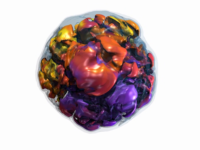
Figure 10: Isoentropy surfaces of the 25-M_⊙ model, painted by Y_e, at 390 milliseconds after bounce. The outer surface is at an entropy per baryon per Boltzmann’s constant of 20. The spatial scale is 500 km on a side. The Y_e colors range from purple ($\sim$0.45), through yellow ($\sim$0.5), to red ($\sim$0.55). This is just after the onset of explosion and portrays the neutrino-driven turbulent structures of the matter behind the shock wave. The top-bottom contrast in the color indicates that there is a hemispheric dependence of the electron-fraction distribution. This is indicative of the LESA phenomenon and is a feature seen in all our exploding models after $\sim$200 milliseconds after bounce.

Figure 10 is a representative depiction of the neutrino-driven bubble structures in our 3D models near the onset of explosion, in this case for the 25-M_⊙ model. Shown are isoentropy surfaces painted by Y_e. A range of scales are visible, with larger scales starting to dominate. Note that there is a distinct color contrast between the top and bottom hemispheres in this model at this time. This Y_e asymmetry is an indirect signature of the LESA phenomenon (Tamborra et al., 2014) and we go into this in more detail in Vartanyan et al. (2019).

3.5 Shock Shape and Structure

One way to characterize and depict the asphericities of the pre- and post-explosion hydrodynamics is to study the spherical harmonic decomposition of the shock wave surface (Burrows et al., 2012). The monopole is the solid-angle-averaged shock radius and the higher-order multipoles reflect the degree of corrugation of this surface in response to turbulent upwelling and distortion during its propagation. It has been shown in the past (Dolence et al., 2013; Vartanyan et al., 2019) that the explosion monopole is accompanied by a dominant dipole, but the exploration of this decomposition for a large, uniform suite of 3D models has not been possible until now. Figure 11 depicts the magnitude of the monopole-normalized dipole (N.B., the dipole is a vector) for the fourteen fiducial models of this paper. There are a few notable aspects of this collection to emphasize. First is that, with individual variation on timescales of tens of milliseconds, all the dipole magnitudes experience a quasi-exponential linear growth phase during the first $\sim$200 ms after bounce, with a time constant (e-folding time) of $\sim$20 ms. This time scales with the advection and sound travel times between the stalled shock at $\sim$150 km and the inner core. Second, the 9-M_⊙ model (red) never achieves a signifcant dipole after explosion, though early in its explosion it seems to be on a trajectory to achieving one. This reflects the near spherical behavior of this explosion, which resembles more a wind driven by the quasi-spherical diffusive flux from the inner core, unaided by much accretion-fueled neutrino power (Burrows et al., 2019, 1995). Third, the shock waves of the non-exploding 13-, 14-, and 15-M_⊙ models retain a much more spherical character than most of the other exploding models, with their dipoles limited to only a $\sim$0.5% effect. The exploding models (except the 9-M_⊙) all achieve a dipole whose magnitude is as much as an order of magnitude larger than seen for the non-exploding models. This distinction between non-exploding and exploding models, except in the case of the 9-M_⊙ model, seems striking and may be robust. Once the non-linear turbulence sets in and vigorous convection is manifest, the subsequent neutrino- and turbulent-pressure-aided explosion almost always assumes a pronounced dipolar component.

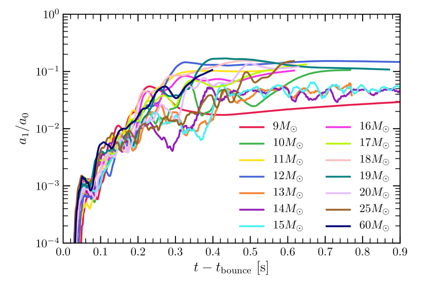
Figure 11: Normalized shock dipole moment. All models show fast growing deformations of the shock. The shock dipole saturation level for exploding models is a factor of a few larger than for failed explosions despite the appearance of the spiral SASI mode for the latter. The 9-M_⊙ progenitor explodes almost spherically and is an exception to this general trend.

We note that the onset of the non-linear turbulent phase will likely depend upon the magnitude and character of the seed perturbations (velocity and thermal fields) in the progenitor. Had we used a different approach to seeding the flow (§2), the details of the developments just described could well have been quantitatively, though probably not qualitatively, different.

Figure 12 depicts the hierarchy of normalized shock multipoles for a representative subset of progenitors. The square root of the sum of the squares of the $m$ subcomponents for each $\ell$, a rotational invariant, is what is plotted. Not only is the prominence of the dipole clearly reinforced, but the various multipoles seem to be nested (by and large) one over the other as a function of spherical harmonic order $\ell$, the highest-order $\ell$ having the lowest magnitude. It is almost as if explosion is correlated with the onset of the growth (as opposed to damped oscillation) of various harmonic mode perturbations of the shock surface, with the growth rates of the $\ell$ modes being a monotonically decreasing function of $\ell$. The $\ell=0$ and $\ell=1$ modes have the greatest rates of growth, and we can see this in the morphologies of the blasts (§3.6). An intriguing future project would be to explore whether this speculation concerning a modal analysis has quantitative merit.

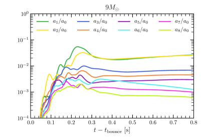
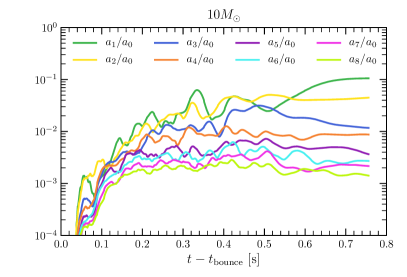
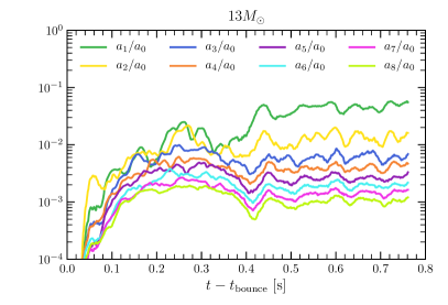
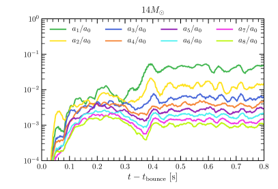
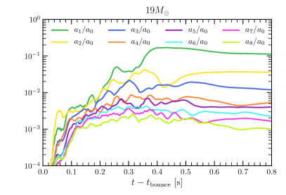
Figure 12: Spherical harmonics decomposition of the shock radius for selected models. All our models show significant deformations of the shock predominantly of dipolar character. The deformations are typically larger for the exploding models, with the exception of the 9-M_⊙ progenitor where the shock front remains close to spherical.

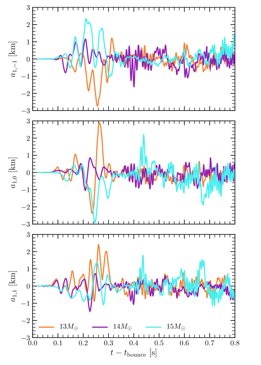
Figure 13: Shock dipole moments for the models that fail to explode. Large spiral-SASI-like oscillations are observed at late times for all the models that do not achieve shock revival.

Another intriguing trend is shown in Figure 13. This figure portrays the dipole subcomponents of the shock surface for the three non-exploding progenitors as a function of time after bounce. The qualitative behavior does not differ from one model to the next. However, there are intriguing features of these plots and models that bear mentioning. The vector amplitudes of all three grow with time in the first $\sim$0.3 seconds, during which the mean shock radius also increases, but after which the magnitude of the dipole subsides. The latter phase marks the shrinkage of the mean shock radius and is near when it becomes clear the model will not explode (at least as the others did). The characteristic pulsation time is of order $\sim$20-25 ms, again comparable to the sound and advection times between the shock and the inner core when the shock is at its greatest extent. Afterwards, with the shrinkage of the shock radius, the characteristic timescale of the subsequent oscillations diminishes to $\sim$10-15 ms. However, the oscillation frequency becomes a bit more regular. What is not obvious from these plots is that the phases of the component oscillations are such that we are witnessing a spiral mode, with the timescale of variation the timescale of the rotation of the mode. This is likely the spiral SASI (Blondin & Shaw, 2007; Foglizzo et al., 2015), and has distinctive gravitational-wave and neutrino-emission signatures (Kuroda et al., 2016; Vartanyan et al., 2019). Otherwise, only for a short interval during the early post-bounce phase of the 25-M_⊙ model do we see the original SASI mode (Blondin et al., 2003; Radice et al., 2019). Moreover, neither the original nor the spiral SASI are in evidence during any of the exploding phases. At least in our calculations, all variants of SASI seem to show up clearly only in the most compact shock configurations. However, whether the spiral SASI leads to a more dynamical later phase (Takiwaki et al., 2016), beyond the horizon of our simulations, seems unlikely, but is yet to be determined.

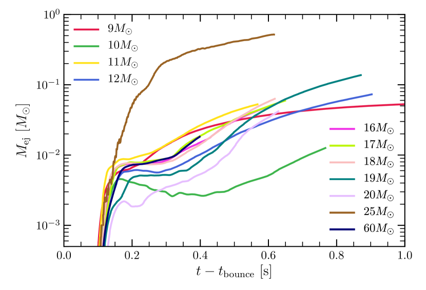
Figure 14: Mass of the material that is not gravitationally bound. Note that for non-exploding models some material is formally unbound for a brief period of time. However, as the shock recedes deeper into the potential well of the PNS, all of the matter behind the shock becomes bound.

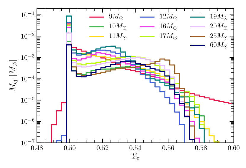
Figure 15: Electron fraction distribution of the ejecta. All models display a peak at $Y_{e}=0.5$ associated with the production of ${}^{56}{\rm Ni}$. Additional abundance peaks are found at different $Y_{e}$’s for different simulations, suggesting that the nucleosynthesis yields might depend on the structure of the imploding stellar cores and show differences between low-compactness and high-compactness progenitors.

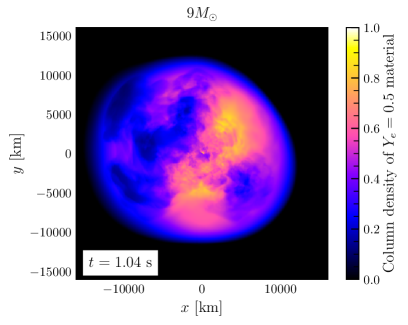
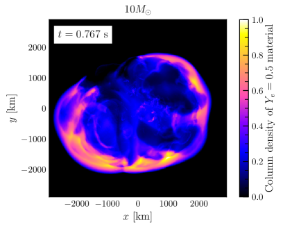
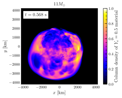
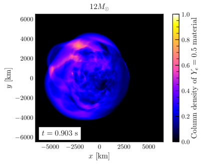
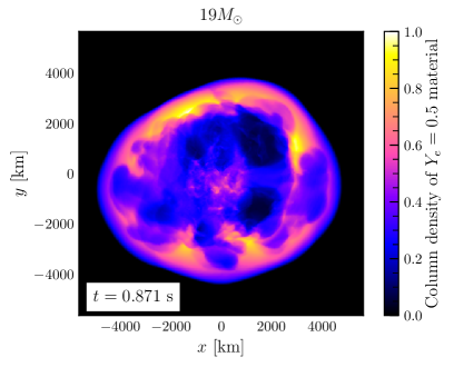
Figure 16: False-color maps of the column density of the Y_e = 0.5 ejecta, wherein ${}^{56}{\rm Ni}$ may reside at the end of the 9-, 10-, 11-, 12-, 19-, and 25-M_⊙ simulations. Note that since we have not performed proper nucleosynthetic calculations these maps are merely notional indications of the approximate positions of whatever ${}^{56}{\rm Ni}$ might be ejected. The ejecta have a complex morphology reminiscent of elemental abundance maps of supernova remnants. However, much longer simulations with nuclear burning and nucleosynthesis turned on are necessary to establish whether or not such similarities are fortuitous.

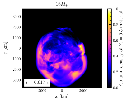
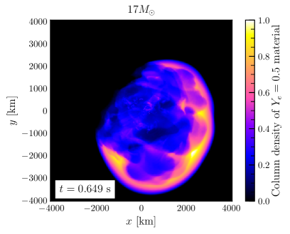
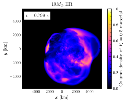
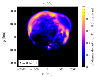
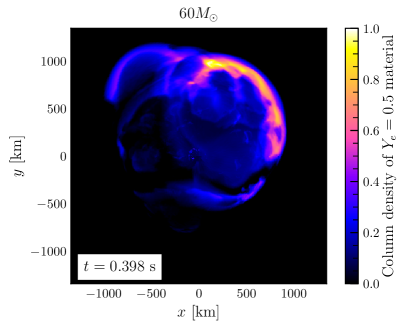
Figure 17: The same as Figure 16, but for the 16-, 17-, 19 (HR)-, 19-, 20-, and 60-M_⊙ simulations. The default 19-M_⊙ model is repeated here for the purpose of direct comparison with its high-resolution variant.

3.6 Ejecta

A calculation should be continued to the end of the explosive phase, at which point the mass cut between the ejecta and the residual neutron star (we surmise, the majority of the time) or black hole would be determined. The ejecta mass and total explosion energy will have then asymptoted (§3.2) to their final values. However, our simulations, except for that for the 9-M_⊙ progenitor, were truncated before asymptoting. Nevertheless, one can still derive general trends in the ejecta mass from the high-density inner region. Recall, that our computational grid extends to 20,000 km. We designate the matter on the grid whose Bernoulli constant (“$\epsilon+P/\rho+v^{2}/2-GM/r$", where “M" is the mass interior to the given radius) is positive as the ejecta mass (M_ej) and track this quantity with time after bounce until the end of a run. Here, $\epsilon$ is the specific internal thermal energy. This number should be a good measure of the outer material of what was the white-dwarf-like progenitor blown off the compact residue in the explosion. It includes the freshly-minted iron-peak material and almost all material processed during explosion by the emerging $\nu_{e}$ and $\bar{\nu}_{e}$ neutrinos. Figure 14 depicts the evolution with time after bounce of M_ej for all the eleven exploding baseline progenitors in this paper. The ejecta masses at the end of each respective simulation range from about a percent of a solar mass to many tenths of a solar mass for the 25-M_⊙ model. The 9-M_⊙ model has asymptoted to $\sim$5$\times$10^-2 solar masses. The 10-M_⊙ model takes a while to reach 10^-2 M_⊙, while the 11-M_⊙ model jumped to $\sim$5$\times$10^-2 M_⊙ early on. The 19-M_⊙ model achieves nearly 0.15 M_⊙ by the end of its run. The 20- and 25-M_⊙ models, the latter taking the most time, eventually experience phases of rapid growth in M_ej. This is due to their shallower initial density profiles (Figure 1) $-$ there is a lot of mass to work with, though this also delays explosion. Similar, but to a lesser degree, are the 16- and 18-M_⊙ models, with M${}_{ej}\sim 0.05$ and $\sim$0.06 M_⊙, respectively.

The electron fraction (Y_e) distributions of these ejecta are given in Figure 15. Most of the ejecta have Y${}_{e}=0.5$ and this material will likely result in radioactive ⁵⁶Ni (and then stable ⁵⁶Fe). However, most of the rest of these inner ejecta have higher Y_es on the proton-rich side. This is the result of net $\nu_{e}$ absorption that exceeds in effect $\bar{\nu}_{e}$ absorption to elevate Y_es above that of symmetric matter. Importantly, this effect depends upon the speed with which the ejecta leave the core. For models, such as the 9-M_⊙ and 12-M_⊙ models, which explode and eject matter quickly, some of the ejecta will not have had time to transition from neutron-rich to proton-rich through the agency of net $\nu_{e}$ neutrino absorption. These models will be a source of some neutron-rich material. At the end of each simulation, these neutron-rich ejecta have reached entropies per baryon per Boltzmann’s constant around $\sim$35 for the 9-M_⊙ model and around $\sim$20 for the 12-M_⊙ model. Those other models that explode later and initially more slowly seem to have enough time to elevate the Y_e of more of their ejecta to proton-rich values. Apart from the disassembly-speed dependence, the fundamental tendency to eject proton-rich material in CCSNe is related to the electron-lepton excess of the PNS. Due to electron-neutrino trapping on infall, there will naturally be a net electron-lepton excess in the emitted neutrinos, which, if given enough time, will push the ejecta Y_e upward. However, the possible effects on this conclusion of neutrino oscillations, not addressed in this study, have yet to be ascertained.

Nevertheless, this progenitor- and explosion-speed dependence is an intriguing conclusion that has important nucleosynthetic consequences. In any case, all our 3D models show a preference for proton-rich ejecta and this, if true, has a consequence for the isotope yields and nucleosynthesis of core-collapse supernovae. Note that this conclusion is contingent upon the proper handling of neutrino transport and is provisional, but is highly suggestive. Similar effects have been seen by Bliss et al. (2018) and Bliss et al. (2018) for PNS winds, and something like a wind component is contributing here. A note of caution, however, is in order. Two-dimensional results for the same progenitors can show different ejecta Y_e distributions that have more neutron-rich ejecta (Vartanyan et al., 2018) (though the ejecta are still predominantly proton-rich). This is mostly a consequence of the different trajectory histories of individual matter parcels during the early explosive phases $-$ 2D and 3D dynamics are not the same, though the neutrino emissions can be similar (see Figure 4 and §3.1).

As noted, however, most of these inner ejecta have a Y_e of 0.5 and we expect this material to include ⁵⁶Ni. We emphasize, however, that we have not performed the necessary nucleosynthesis calculations, nor incorporated tracer particles to facilitate such calculations, and have left this to future work. Figures 16 and 17 show column density maps of the “Y_e = 0.5" regions wherein we expect whatever ⁵⁶Ni that is created for a sample of our exploding models to reside. These figures should not be interpreted to indicate perfectly our produced ⁵⁶Ni, but merely to indicate in a rough fashion where we expect it to reside. The distributions vary significantly from model to model, some having roughly symmetric angular distributions and others very asymmetrical angular distributions. All, however, have shells of ⁵⁶Ni and are not fully filled in. Both these observations may have consequences for the observed distributions of the iron-peak elements in supernova light curves, spectra (via line profiles), and remnants.

4 Brief Sensitivity Investigation

It is important to gauge the sensitivity of simulation results to variations in input physics and methodologies; it is in this way that the qualitative import of uncertainties in the relevant physics and of approximations in the numerical schemes can be ascertained. To this end, there is already a large literature spanning decades wherein the dependence of CCSN dynamics on changes in the physics has been inspected. However, given the complexity of the overall core-collapse supernova simulation enterprise, this is not something easily determined nor quantified. Nevertheless, such efforts are ongoing and modern codes incorporate many of the lessons learned.

There have not, however, been many such studies to determine the consequences of such alterations in the context of full 3D simulations. Until recently, this would have been prohibitively expensive. In this section, we provide a few such comparisons, altering only a few aspects of 3D simulations. These include the angular spatial resolution, the effect of the Horowitz et al. (2017) many-body correction to the axial-vector term in the neutrino-nucleon scattering rates, and the use of a monopole versus a multipole (Müller & Steinmetz, 1995) gravity expansion. Nagakura et al. (2019), to which the reader is referred, have provided more details and interpretation for the angular resolution study of the 19-M_⊙ model, but here we augment that study with a few additional observations. In addition, we contrast the behavior of 3D models with and without the many-body correction for both the same 19-M_⊙ progenitor and our 11-M_⊙ progenitor, at our standard resolution (§2). The 19-M_⊙ progenitor is also the context of our single multipole/monopole comparison.

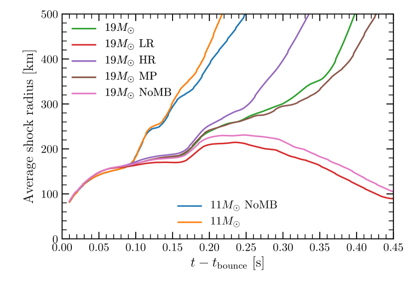
Figure 18: Shock radius evolution for the 11-M_⊙ and 19-M_⊙ progenitors, with and without many-body corrections to the neutrino-nucleon scattering cross section. The inclusion of many-body effects is crucial for the explosion of the 19-M_⊙ progenitor, and strengthens the explosion of the 11-M_⊙ progenitor.

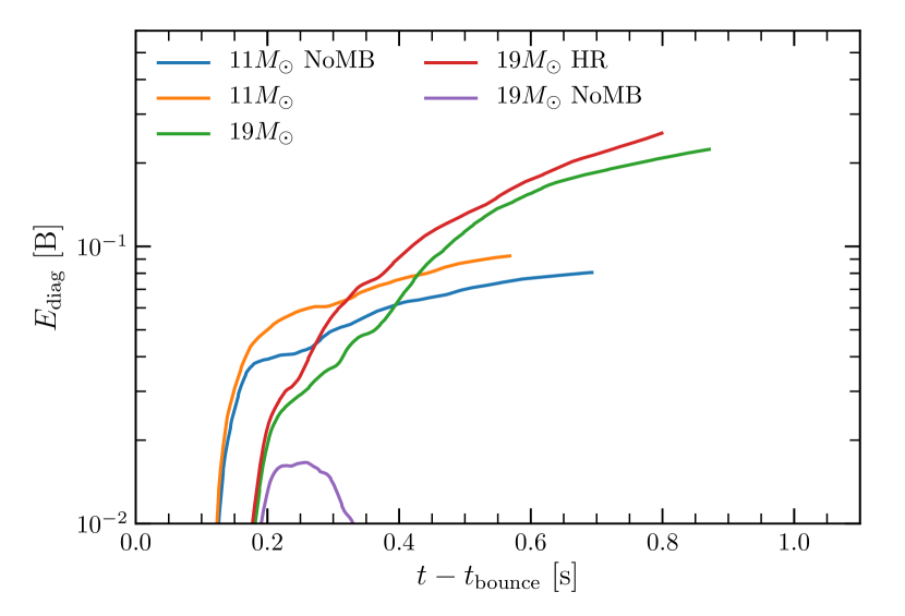
Figure 19: Diagnostic explosion energy for the 11-M_⊙ and 19-M_⊙ progenitors, with and without many-body corrections to the neutrino nucleon scattering cross-section. See the text for a discussion.

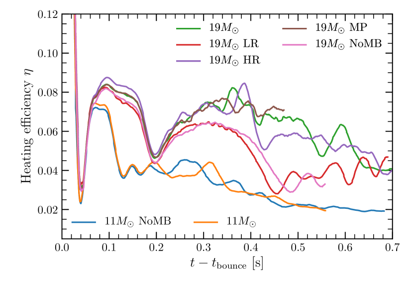
Figure 20: Heating efficiencies for the 11-M_⊙ and 19-M_⊙ progenitors, with and without many-body corrections to the neutrino-nucleon scattering cross section. The inclusion of many-body effects leads to a more rapid contraction of the PNS, resulting in slightly higher neutrino rms energies, and, consequently, higher heating efficiencies. See text for a discussion.

Figure 18 provides a comparison of the evolution of the mean shock radius with time after bounce for all the models in our modest sensitivity study. From a comparison of models 19-M_⊙ (default: 678$\times$128$\times$256, green), 19-M_⊙-LR (low-resolution: 678$\times$64$\times$128, red), and 19-M_⊙-HR (high-resolution: 678$\times$256$\times$512, purple) we see that if the resolution is too low a model that otherwise explodes will not. This is, of course, a qualitative difference and is explained and analyzed in more detail in Nagakura et al. (2019). The increased numerical viscosity at lower resolution inhibits the turbulent pressure important in almost all neutrino-driven models of explosion. We also see that the higher resolution model explodes earlier. This result puts a premium on spatial resolution as a factor in the interpretation of model results in the literature. We note that this 19-M_⊙-HR model is one of the highest resolution 3D supernova models ever performed using a spherical grid.

From Figure 18, we learn that, whereas the many-body correction makes little qualitative difference for the 11-M_⊙ progenitor (11-M_⊙ versus 11-M_⊙-NoMB), without it (19-M_⊙-NoMB, magenta) our otherwise default 3D 19-M_⊙ model does not explode. The density profile of the 11-M_⊙ progenitor all but ensures explosion for a range of microphysics, but to get the 19-M_⊙ model (and, presumably, other more massive progenitors) to explode the many-body correction, as we have currently implemented it (Horowitz et al., 2017), has proven supportive. The many-body effect decreases slightly the neutrino-nucleon scattering rate, thereby accelerating the shrinkage of the core. This raises by the resulting compression the temperatures around the $\nu_{e}$ and $\bar{\nu}_{e}$ neutrinospheres and, as a result, the heating rates due to absorption on nucleons near the stalled shock wave. This facilitates explosion. What the effect may be of anticipated improvements down the road in this class of corrections is yet to be determined (Burrows & Sawyer, 1998, 1999; Roberts et al., 2012; Roberts & Reddy, 2017).

Also on Figure 18, we find that there is little difference between models using the full multipole gravitational expansion (19-M_⊙-MP) and those that retain only the monopole. This is due to the strong central concentration of the generic core-collapse structure and the fact that all our initial models are non-rotating.

Figure 19 plots the evolution with time after bounce of the diagnostic energy of exploding models. We see that the many-body correction increases the explosion energy of the 11-M_⊙ progenitor by $\sim$20% and that higher resolution does the same (at least in this comparison study) for the 19-M_⊙ model. These are not qualitative differences, but important ones, as we attempt to determine, or at least bracket, the salient quantities of theoretical CCSN explosions.

Figure 20 displays the heating efficiencies ($\eta$) for all our sensitivity calculations. The efficiency is defined as the ratio of the neutrino power deposition rate by $\nu_{e}$ and $\bar{\nu}_{e}$ absorption in the gain region behind the shock wave and the sum of the angle- and group-integrated $\nu_{e}$ and $\bar{\nu}_{e}$ luminosities. This number does not include the subdominant heating rate due to inelastic scattering, though the simulations do. $\eta$ is approximately a measure of the “optical depth" to neutrino absorption and ranges from $\sim$4% to $\sim$8%. Core-collapse supernovae are a “5$-$10-%" effect, not the “$\sim$1%" effect often quoted. We see that during the first $\sim$0.2 seconds there is little difference between the various models with the same progenitor mass. The high-resolution 19-M_⊙ model does have a slightly higher energy deposition rate than the default model, and higher still than the low-resolution realization. This is one of the reasons for the qualitative difference in the outcomes (HR versus LR) (Nagakura et al., 2019). In addition, the default 11-M_⊙ model with the many-body correction has a $\sim$3% higher heating rate early on, but in a time-averaged sense is not much different after explosion. Not unexpectedly, the comparison between the two models with and without the higher-order multipole gravity terms reveals no appreciable differences. One thing we do notice is that the efficiency is not a good predictor or index of explosion, since models such as 19-M_⊙-NoMB and 19-M_⊙-LR have approximately the same $\eta$ history, but only one explodes, and the $\eta$ values for the two non-exploding 19-M_⊙ models are higher than those for the exploding 11-M_⊙ models.

The small set of 3D simulations we have performed here to address some sensitivity issues can not in any way be construed as definitive, nor adequate to the general task of exploring the important dependences of CCSN theory on the outstanding ambiguities concerning progenitors, microphysics, resolution, and numerical technique. This is the ongoing program for the community of supernova theorists. However, ours are some of the first to be performed in 3D with a state-of-the-art supernova code, and, as such, are meant in part to indicate what is now possible.

5 Conclusions

For this paper, we have conducted and assembled for analysis nineteen state-of-the-art 3D core-collapse supernova simulations spanning a broad range of progenitor masses and structures. This is, we believe, the largest such collection of sophisticated 3D supernova simulations ever performed. A goal was to determine the behavior of the family of CCSN progenitors, not just one model at a time, but collectively, and to determine overarching trends vis à vis explodability and outcomes. We have found that while the majority of this suite explode, not all do, and that even models in the middle of the available progenitor mass range may be less explodable. This does not mean that those models for which we did not witness explosion would not explode in Nature, but that they are less prone to explosion than others in this cohort. One clear consequence is that the “compactness" measure is not a metric for explodability $-$ we, find as have others (Ugliano et al., 2012; Perego et al., 2015; Ertl et al., 2016), that models with both low and high compactness can explode, but that some with an intermediate value may not. As we have discussed in previous work (Burrows et al., 2018), since a core-collapse supernova explosion is a critical bifurcation, explodability is still sensitive to the detailed microphysics and numerical schema. Despite our attempts here to incorporate the necessary realism and address all the major issues with the latest methods and physics, every feature of our Fornax implementation and simulations should be considered provisional. The supernova theory community continues its decades-long investigations into neutrino-matter interactions, the nuclear equation of state, and massive star evolution and progenitors with the goal of obtaining a robust understanding of the core-collapse supernova phenomenon. This paper, though it contains an unprecedentedly large set of 3D CCSN simulations, is but one contribution to this ongoing collective effort.

We found that a preponderance of lower-mass massive star progenitors likely experience lower-energy explosions, while the higher-mass massive stars likely experience higher-energy explosions. The latter explode a bit latter after bounce than the former, so time of explosion seems weakly correlated or anti-correlated with explosion vigor. However, this is a statistical statement and we have not determined the full range of possible explosion energies for a given progenitor in the context of chaotic turbulence and chaotic initial models. Not unexpectedly, we confirm in 3D that neutrino-driven turbulence behind the stalled shock wave is a major factor in the viability of the neutrino-driven mechanism of CCSN. Moreover, as was determined in Vartanyan et al. (2019) and Burrows et al. (2019), most 3D models have a dominant dipole morphology, have a pinched, wasp-waist early structure, and experience simultaneous accretion and explosion. Continuing accretion during explosion maintains the neutrino power during the crucial early launch phase.

Coupled with the earlier calculations of Radice et al. (2017) concerning the sources from $\sim$8$-$8.8 M_⊙ progenitors of the lowest-mass pulsars (down to $\sim$1.17 M_⊙ gravitational; (Martinez et al., 2015)), we have now been able to reproduce in a qualitative sense the general range of residual neutron-star masses inferred for the galactic neutron-star population. However, the mapping of massive star mass function to initial neutron star mass function has not been attempted and is likely a job for the future. One of our most important conclusions is that the most massive progenitor models need to be continued for longer physical times, perhaps to many seconds, to asymptote to a final state, in particular vis à vis explosion energy. This seems to be a firm conclusion of our 3D study, and was anticipated by Müller (2015). Moreover, we find that while the majority of the inner ejecta have Y${}_{e}=0.5$, there is a substantial proton-rich tail. Those models that explode more lethargically and a bit later after bounce tend not to include much neutron-rich ejecta, while those that explode more quickly, such as the lowest-mass progenitors (e.g., the 9-M_⊙ model), can ejecta some more neutron-rich matter. However, in all our 3D models, the inner ejecta have a net proton-richness. If true, this systematic result has important consequences for the nucleosynthetic yields as a function of progenitor.

We find that the non-exploding models eventually evolve into compact inner configurations that experience a quasi-periodic spiral SASI mode. We otherwise see little evidence of the SASI in the exploding models, except during a brief period at early post-bounce times for the 25-M_⊙ model. For the latter model, the slightly smaller initial post-bounce shock radius, by dint of the greater early accretion it experiences, is likely responsible for this transient phase.

We are now in a position to articulate the features of a progenitor and physics model supportive of explosion. Foremost, perhaps, is the initial progenitor mass density profile $-$ all else being equal, such structures determine the outcomes of collapse. Associated is the seed perturbation field inherited from the pre-collapse core. Jump starting and continuing to seed turbulent convection behind the stalled shock wave is necessary for a vigorous outcome, though the detailed character of the requisite seed turbulence has yet to be determined. Along with these two aspects of a progenitor is a third, the presence of a sharp silicon/oxygen interface. We here and elsewhere (Vartanyan et al., 2018) confirm that explosion is ofttimes inaugurated upon accretion of this interface. There is a delay of tens of milliseconds between accretion through the shock and the response of the emergent neutrino luminosities to the consequent decrease in accretion rate, with the result that the countervailing effect of the accretion ram pressure is temporarily diminished. The upshot is often explosion.

Though we have not addressed this in this paper, increasing the mean dwell time in the gain region of a given parcel of newly-shocked matter increases the exposure of that parcel to neutrino heating and facilitates explosion (Murphy & Burrows, 2008). Turbulence behind the stalled shock wave does just this, and such an enhancement is one positive feature of multi-dimensional motions absent in spherical models. However, as has been made clear in numerous publications, the Reynolds stress itself of the neutrino-driven convection behind the shock wave contributes centrally to explosion and may be the most important aspect of multi-dimensional turbulent motion. Converting some of the accretion gravitational energy into turbulence channels energy into a component (turbulence) that, if it were a gas, would have an effective $\gamma$ of $\sim$2 (not $4/3$) and would be anisotropic in the radial direction (Murphy & Burrows, 2008). This means that turbulence is an effective means to generate needed outward “pressure" stress (Burrows et al., 1995; Couch & Ott, 2015; Nagakura et al., 2019) behind the shock wave. Turbulence, hence, is more effective than fluid pressure for the same energy density.

Of course, central to the neutrino mechanism of core-collapse supernova explosions is the power deposited by the $\nu_{e}$ and $\bar{\nu}_{e}$ neutrinos in the gain region behind the shock $-$ this is the ultimate source of the supernova energy when the rotation rate is small. Though charged-current absorption on nucleons dominates this rate, inelastic neutrino-electron and neutrino-nucleon scattering play positive roles, perhaps in aggregate by as much as $\sim$10$-$15% (Burrows et al., 2018). The large energy transfer of neutrino-electron scattering happens at a small rate and the small energy transfer of neutrino-nucleon scattering occurs at a more rapid rate. The upshot is a comparable (to within a factor of $\sim$2) contribution, though neutrino-electron scattering seems generally more important.

The many-body correction of Horowitz et al. (2017) to the axial-vector term in neutral-current neutrino-nucleon scattering is also a factor. In particular, the resultant decreased interaction cross sections for such scattering lead to a more rapid loss of $\nu_{\mu}$, $\bar{\nu}_{\mu}$, $\nu_{\tau}$, and $\bar{\nu}_{\tau}$ neutrinos. This accelerates the contraction of the inner core, with the result that the temperatures around the $\nu_{e}$ and $\bar{\nu}_{e}$ neutrinospheres are increased. Increased temperatures harden their emergent spectra and, since the rate of charged-current absorption goes as the square of the neutrino energy, the heating rates in the gain region increase. Therefore, and ironically, enhanced energy leakage into a less productive channel (the “$\nu_{\mu}$s") facilitates explosion. This is similar to the published effect of general-relativity $-$ despite the redshifting of the emergent neutrinos and the deeper potential well, more compact relativistic configurations aid explosion (Bruenn et al., 2001; Müller et al., 2012). However, the full set of many-body corrections has not yet been calculated (Burrows & Sawyer, 1998, 1999; Roberts et al., 2012; Roberts & Reddy, 2017) nor implemented, so their ultimate effect has yet to be determined.

We also note that PNS convection in the inner core around $\sim$20$\pm 5$ km increases the “$\nu_{\mu}$" loss rate, performing, though to a lesser degree, a similar function to that of the many-body correction (Radice et al., 2017). The effect is similar in both 2D and 3D simulations (H. Nagakura et al., in preparation).

The nuclear EOS is a perennial central issue. Fischer et al. (2018) have explored the possible effects of a quark-hadron phase transition at super-nuclear densities. Schneider et al. (2019) have shown that a higher effective neutron mass near nuclear density can aid explosion, through its effect on nuclear specific heats and, hence, on the temperatures achieved during and after collapse. The EOS we have employed (SFHo) has an effective mass near 0.7$\times$$m_{n}$, while Schneider et al. (2019) find that values close to 1.0$\times$$m_{n}$, such as are found in the LS220 EOS (Lattimer & Douglas Swesty, 1991), could support greater explodability. However, the LS220 EOS and such a high effective mass currently seem incompatible with known nuclear constraints (Tews et al., 2017). Another physical effect that may have some bearing on the question of explodablity and that has an indirect EOS connection is the electron capture rate during infall (Sullivan et al., 2016; Titus et al., 2018; Nagakura et al., 2019). This rate depends upon the free proton abundance, an EOS-dependent quantity that, along with the capture rate on heavy nuclei, determines the rate of electron loss. The loss of electrons translates into a loss of pressure that affects the rate of collapse and time to bounce. Hence, variations in the total capture rate result in variations in the time to bounce (Lentz et al., 2012). Since alterations in the time to bounce affect the timing of the subsequent mass accretion of the outer core onto the inner core, and the $\dot{M}$ history factors into the explodability, scrutiny of these issues in the future could bear fruit. In addition, the stiffness of the EOS at high density will help determine the size of the inner core, the depth of the gravitational potential well, and the neutrinopshere temperatures. These factors influence the work against gravity needed to launch the ejecta, as well as the neutrino deposition powers in the gain region. So, there remain issues surrounding the nuclear EOS, not addressed in this paper, that could prove illuminating.

Finally, we have not in this paper looked into the possible effects of rotation and/or magnetic fields. The latter, if the core is not rotating fast, are unlikely to alter our findings to an interesting degree. Magneto-turbulence will be similar to hydrodynamic turbulence as far as aggregate stress is concerned. Rapid differential rotation, on the other hand, has the potential to generate large magnetic stresses (Burrows et al., 2007; Mösta et al., 2014; Obergaulinger & Aloy, 2019), with the result that strong jets can emerge. However, it is thought that most pulsars are not born rotating fast (Faucher-Giguère & Kaspi, 2006) and that the majority of CCSNe are not magneto-rotationally powered. Nevertheless, it remains to determine whether even slow or modest rotation has a role to play in the overall context of CCSNe. An intriguing possibility is that even slow rotation might promote our recalcitrant 13-, 14-, and 15-M_⊙ models into explosion.

With the advent of Fornax and the ongoing development of an international constellation of full-physics codes, multiple 3D simulations per year are now the new standard in core-collapse theory. Not only does this finally ensure an extensive exploration of parameter space in the full three dimensions of Nature, but it mitigates the resource penalties of the few inevitable mistakes. Though much remains to be done, as a result of this extensive study using Fornax, we can now feel confident that a decades-long theoretical challenge is finally yielding many of its secrets.

References

- Antoniadis et al. (2013) Antoniadis J., Freire P. C. C., Wex N., Tauris T. M., Lynch R. S., van Kerkwijk M. H., Kramer M., 2013, Science, 340, 448
- Bethe & Wilson (1985) Bethe H. A., Wilson J. R., 1985, ApJ, 295, 14
- Bionta et al. (1987) Bionta R. M., Blewitt G., Bratton C. B., Casper D. Kropp W. R., Learned J. G., Losecco J. M., 1987, Phys. Rev. Lett., 58, 1494
- Bliss et al. (2018) Bliss J., Arcones A., Qian Y.-Z., 2018, ApJ, 866, 105
- Bliss et al. (2018) Bliss J., Witt M., Arcones A., Montes F., Pereira J., 2018, ApJ, 855, 135
- Blondin et al. (2003) Blondin J. M., Mezzacappa A., DeMarino C., 2003, ApJ, 584, 971
- Blondin & Shaw (2007) Blondin J. M., Shaw S., 2007, ApJ, 656, 366
- Bruenn et al. (2001) Bruenn S. W., De Nisco K. R., Mezzacappa A., 2001, ApJ, 560, 326
- Bruenn et al. (2016) Bruenn S. W., Lentz E. J., Hix W. R., Mezzacappa A., Harris J. A., Messer O. E. B., Endeve E., Blondin J. M., Chertkow M. A., Lingerfelt E. J., Marronetti P., Yakunin K. N., 2016, ApJ, 818, 123
- Burrows et al. (2007) Burrows A., Dessart L., Livne E., Ott C. D., Murphy J., 2007, ApJ, 664, 416
- Burrows et al. (2012) Burrows A., Dolence J. C., Murphy J. W., 2012, ApJ, 759, 5
- Burrows et al. (1995) Burrows A., Hayes J., Fryxell B. A., 1995, ApJ, 450, 830
- Burrows & Lattimer (1986) Burrows A., Lattimer J. M., 1986, ApJ, 307, 178
- Burrows et al. (2019) Burrows A., Radice D., Vartanyan D., 2019, MNRAS, 485, 3153
- Burrows et al. (2006) Burrows A., Reddy S., Thompson T. A., 2006, Nuclear Physics A, 777, 356
- Burrows & Sawyer (1998) Burrows A., Sawyer R. F., 1998, Phys. Rev. C, 58, 554
- Burrows & Sawyer (1999) Burrows A., Sawyer R. F., 1999, Phys. Rev. C, 59, 510
- Burrows & Thompson (2004) Burrows A., Thompson T. A., 2004, in Fryer C. L., ed., Astrophysics and Space Science Library Vol. 302 of Astrophysics and Space Science Library, Neutrino-Matter Interaction Rates in Supernovae. pp 133–174
- Burrows et al. (2018) Burrows A., Vartanyan D., Dolence J. C., Skinner M. A., Radice D., 2018, Space Sci. Rev., 214, 33
- Chatzopoulos et al. (2016) Chatzopoulos E., Couch S. M., Arnett W. D., Timmes F. X., 2016, ApJ, 822, 61
- Couch (2013) Couch S. M., 2013, Astrophys. J., 765, 29
- Couch et al. (2015) Couch S. M., Chatzopoulos E., Arnett W. D., Timmes F. X., 2015, ApJ, 808, L21
- Couch & Ott (2015) Couch S. M., Ott C. D., 2015, ApJ, 799, 5
- Cromartie et al. (2019) Cromartie H. T., Fonseca E., Ransom S. M., et al. 2019, Nature Astronomy, p. 439
- da Silva Schneider et al. (2017) da Silva Schneider A., Roberts L. F., Ott C. D., 2017, arXiv e-prints, p. arXiv:1707.01527
- Demorest et al. (2010) Demorest P. B., Pennucci T., Ransom S. M., Roberts M. S. E., Hessels J. W. T., 2010, Nature, 467, 1081
- Dessart et al. (2006) Dessart L., Burrows A., Livne E., Ott C. D., 2006, ApJ, 645, 534
- Dolence et al. (2013) Dolence J. C., Burrows A., Murphy J. W., Nordhaus J., 2013, ApJ, 765, 110
- Eldridge et al. (2019) Eldridge J. J., Guo N.-Y., Rodrigues N., Stanway E. R., Xiao L., 2019, arXiv e-prints
- Ertl et al. (2016) Ertl T., Janka H. T., Woosley S. E., Sukhbold T., Ugliano M., 2016, ApJ, 818, 124
- Faucher-Giguère & Kaspi (2006) Faucher-Giguère C.-A., Kaspi V. M., 2006, ApJ, 643, 332
- Fischer et al. (2018) Fischer T., Bastian N.-U. F., Wu M.-R., Baklanov P., Sorokina E., Blinnikov S., Typel S., Klähn T., Blaschke D. B., 2018, Nature Astronomy, 2, 980
- Foglizzo et al. (2015) Foglizzo T., Kazeroni R., Guilet J., Masset F., González M., Krueger B. K., Novak J., Oertel M., Margueron J., Faure J., Martin N., Blottiau P., Peres B., Durand G., 2015, Publ. of the Astron. Soc. of Australia, 32, e009
- Glas et al. (2019) Glas R., Just O., Janka H.-T., Obergaulinger M., 2019, ApJ, 873, 45
- Hanawa et al. (2008) Hanawa T., Mikami H., Matsumoto T., 2008, Journal of Computational Physics, 227, 7952
- Hempel et al. (2012) Hempel M., Fischer T., Schaffner-Bielich J., Liebendörfer M., 2012, ApJ, 748, 70
- Hirata et al. (1987) Hirata K., Kajita T., Koshiba M., Nakahata M., Oyama Y., Sato N., Suzuki A., Takita M., 1987, Phys. Rev. Lett., 58, 1490
- Horowitz (2002) Horowitz C. J., 2002, Phys. Rev. D, 65, 043001
- Horowitz et al. (2017) Horowitz C. J., Caballero O. L., Lin Z., O’Connor E., Schwenk A., 2017, Phys. Rev. C, 95, 025801
- Janka (2017) Janka H.-T., 2017, Neutrino-Driven Explosions. Springer International Publishing AG, p. 1095
- Jones et al. (2019) Jones S., Röpke F. K., Fryer C., Ruiter A. J., Seitenzahl I. R., Nittler L. R., Ohlmann S. T., Reifarth R., Pignatari M., Belczynski K., 2019, A&A, 622, A74
- Jones et al. (2016) Jones S., Röpke F. K., Pakmor R., Seitenzahl I. R., Ohlmann S. T., Edelmann P. V. F., 2016, A&A, 593, A72
- Juodagalvis et al. (2010) Juodagalvis A., Langanke K., Hix W. R., Martínez-Pinedo G., Sampaio J. M., 2010, Nuclear Physics A, 848, 454
- Kuroda et al. (2016) Kuroda T., Kotake K., Takiwaki T., 2016, ApJ, 829, L14
- Lai & Goldreich (2000) Lai D., Goldreich P., 2000, ApJ, 535, 402
- Lattimer & Douglas Swesty (1991) Lattimer J. M., Douglas Swesty F., 1991, Nuclear Physics A, 535, 331
- Lattimer & Prakash (2007) Lattimer J. M., Prakash M., 2007, Phys. Rep., 442, 109
- Lentz et al. (2015) Lentz E. J., Bruenn S. W., Hix W. R., Mezzacappa A., Messer O. E. B., Endeve E., Blondin J. M., Harris J. A., Marronetti P., Yakunin K. N., 2015, ApJ, 807, L31
- Lentz et al. (2012) Lentz E. J., Mezzacappa A., Messer O. E. B., Liebendörfer M., Hix W. R., Bruenn S. W., 2012, ApJ, 747, 73
- Marek et al. (2006) Marek A., Dimmelmeier H., Janka H. T., Müller E., Buras R., 2006, A&A, 445, 273
- Martinez et al. (2015) Martinez J. G., Stovall K., Freire P. C. C., Deneva J. S., Jenet F. A., McLaughlin M. A., Bagchi M., Bates S. D., Ridolfi A., 2015, Astrophys. J., 812, 143
- Martinez & Bersten (2019) Martinez L., Bersten M. C., 2019, arXiv e-prints
- Mayle et al. (1987) Mayle R., Wilson J. R., Schramm D. N., 1987, ApJ, 318, 288
- Melson et al. (2015) Melson T., Janka H.-T., Bollig R., Hanke F., Marek A., Müller B., 2015, ApJ, 808, L42
- Morozova et al. (2018) Morozova V., Piro A. L., Valenti S., 2018, ApJ, 858, 15
- Mösta et al. (2014) Mösta P., Richers S., Ott C. D., Haas R., Piro A. L., Boydstun K., Abdikamalov E., Reisswig C., Schnetter E., 2014, ApJ, 785, L29
- Müller (2015) Müller B., 2015, MNRAS, 453, 287
- Müller & Janka (2015) Müller B., Janka H.-T., 2015, MNRAS, 448, 2141
- Müller et al. (2010) Müller B., Janka H.-T., Dimmelmeier H., 2010, ApJS, 189, 104
- Müller et al. (2012) Müller B., Janka H.-T., Marek A., 2012, ApJ, 756, 84
- Müller et al. (2017) Müller B., Melson T., Heger A., Janka H.-T., 2017, MNRAS, 472, 491
- Müller et al. (2019) Müller B., Tauris T. M., Heger A., Banerjee P., Qian Y.-Z., Powell J., Chan C., Gay D. W., Langer N., 2019, MNRAS, 484, 3307
- Müller & Steinmetz (1995) Müller E., Steinmetz M., 1995, Computer Physics Communications, 89, 45
- Murphy & Burrows (2008) Murphy J. W., Burrows A., 2008, Astrophys. J., 688, 1159
- Nagakura et al. (2019) Nagakura H., Burrows A., Radice D., Vartanyan D., 2019, arXiv e-prints
- Nagakura et al. (2019) Nagakura H., Furusawa S., Togashi H., Richers S., Sumiyoshi K., Yamada S., 2019, ApJS, 240, 38
- Nagakura et al. (2018) Nagakura H., Iwakami W., Furusawa S., Okawa H., Harada A., Sumiyoshi K., Yamada S., Matsufuru H., Imakura A., 2018, ApJ, 854, 136
- Nagakura et al. (2017) Nagakura H., Iwakami W., Furusawa S., Sumiyoshi K., Yamada S., Matsufuru H., Imakura A., 2017, ApJS, 229, 42
- Nagakura et al. (2014) Nagakura H., Sumiyoshi K., Yamada S., 2014, ApJS, 214, 16
- Nagakura et al. (2019) Nagakura H., Sumiyoshi K., Yamada S., 2019, ApJ, 878, 160
- Obergaulinger & Aloy (2019) Obergaulinger M., Aloy M. Á., 2019, arXiv e-prints, p. arXiv:1909.01105
- O’Connor et al. (2018) O’Connor E., Bollig R., Burrows A., Couch S., Fischer T., Janka H.-T., Kotake K., Lentz E. J., Liebendörfer M., Messer O. E. B., Mezzacappa A., Takiwaki T., Vartanyan D., 2018, Journal of Physics G Nuclear Physics, 45, 104001
- O’Connor & Ott (2013) O’Connor E., Ott C. D., 2013, ApJ, 762, 126
- O’Connor & Couch (2018) O’Connor E. P., Couch S. M., 2018, ApJ, 865, 81
- O’Connor & Couch (2018) O’Connor E. P., Couch S. M., 2018, Astrophys. J., 854, 63
- Perego et al. (2015) Perego A., Hempel M., Fröhlich C., Ebinger K., Eichler M., Casanova J., Liebendörfer M., Thielemann F. K., 2015, ApJ, 806, 275
- Poznanski (2013) Poznanski D., 2013, MNRAS, 436, 3224
- Radice et al. (2017) Radice D., Burrows A., Vartanyan D., Skinner M. A., Dolence J. C., 2017, ApJ, 850, 43
- Radice et al. (2019) Radice D., Morozova V., Burrows A., Vartanyan D., Nagakura H., 2019, ApJ, 876, L9
- Rampp & Janka (2002) Rampp M., Janka H.-T., 2002, A&A, 396, 361
- Roberts & Reddy (2017) Roberts L. F., Reddy S., 2017, Phys. Rev. C, 95, 045807
- Roberts et al. (2012) Roberts L. F., Reddy S., Shen G., 2012, Phys. Rev. C, 86, 065803
- Schneider et al. (2019) Schneider A. S., Roberts L. F., Ott C. D., O’Connor E., 2019, arXiv e-prints
- Skinner et al. (2016) Skinner M. A., Burrows A., Dolence J. C., 2016, ApJ, 831, 81
- Skinner et al. (2019) Skinner M. A., Dolence J. C., Burrows A., Radice D., Vartanyan D., 2019, ApJS, 241, 7
- Souza et al. (2009) Souza S. R., Steiner A. W., Lynch W. G., Donangelo R., Famiano M. A., 2009, ApJ, 707, 1495
- Steiner et al. (2013) Steiner A. W., Hempel M., Fischer T., 2013, ApJ, 774, 17
- Sukhbold et al. (2016) Sukhbold T., Ertl T., Woosley S. E., Brown J. M., Janka H. T., 2016, ApJ, 821, 38
- Sukhbold et al. (2018) Sukhbold T., Woosley S. E., Heger A., 2018, ApJ, 860, 93
- Sullivan et al. (2016) Sullivan C., O’Connor E., Zegers R. G. T., Grubb T., Austin S. M., 2016, ApJ, 816, 44
- Summa et al. (2018) Summa A., Janka H.-T., Melson T., Marek A., 2018, ApJ, 852, 28
- Suwa et al. (2013) Suwa Y., Takiwaki T., Kotake K., Fischer T., Liebendörfer M., Sato K., 2013, Astrophys. J., 764, 99
- Takahashi & Yamada (2014) Takahashi K., Yamada S., 2014, ApJ, 794, 162
- Takiwaki et al. (2016) Takiwaki T., Kotake K., Suwa Y., 2016, MNRAS, 461, L112
- Tamborra et al. (2014) Tamborra I., Hanke F., Janka H.-T., Müller B., Raffelt G. G., Marek A., 2014, ApJ, 792, 96
- Tews et al. (2017) Tews I., Lattimer J. M., Ohnishi A., Kolomeitsev E. E., 2017, ApJ, 848, 105
- Thompson et al. (2000) Thompson T. A., Burrows A., Horvath J. E., 2000, Phys. Rev. C, 62, 035802
- Thompson et al. (2003) Thompson T. A., Burrows A., Pinto P. A., 2003, ApJ, 592, 434
- Titus et al. (2018) Titus R., Sullivan C., Zegers R. G. T., Brown B. A., Gao B., 2018, Journal of Physics G Nuclear Physics, 45, 014004
- Ugliano et al. (2012) Ugliano M., Janka H.-T., Marek A., Arcones A., 2012, ApJ, 757, 69
- Vartanyan et al. (2019) Vartanyan D., Burrows A., Radice D., 2019, MNRAS, p. 2235
- Vartanyan et al. (2018) Vartanyan D., Burrows A., Radice D., Skinner M. A., Dolence J., 2018, MNRAS, 477, 3091
- Vartanyan et al. (2019) Vartanyan D., Burrows A., Radice D., Skinner M. A., Dolence J., 2019, MNRAS, 482, 351
- Vaytet et al. (2011) Vaytet N. M. H., Audit E., Dubroca B., Delahaye F., 2011, Journal of Quantitative Spectroscopy and Radiative Transfer, 112, 1323
- Woosley (2019) Woosley S. E., 2019, ApJ, 878, 49
- Woosley & Heger (2007) Woosley S. E., Heger A., 2007, Phys. Rep., 442, 269
- Yamamoto et al. (2013) Yamamoto Y., Fujimoto S., Nagakura H., Yamada S., 2013, ApJ, 771, 27
- Yoshida et al. (2019) Yoshida T., Takiwaki T., Kotake K., Takahashi K., Nakamura K., Umeda H., 2019, arXiv e-prints