Kubo conductivity for anisotropic tilted Dirac semimetals and its application to 8-Pmmn borophene:
The role of different frequency, temperature and scattering limits

Abstract

The electronic and optical conductivities for anisotropic tilted Dirac semimetals are calculated using the Kubo formula. As in graphene, it is shown that the minimal conductivity is sensitive to the order in which the temperature, frequency and scattering limits are taken. Both intraband and interband scattering are found to be direction dependent. In the high frequency and low temperature limit, the conductivities do not depend on frequency and are weighted by the anisotropy in such a way that the geometrical mean $\sqrt{\sigma_{xx}\sigma_{yy}}$ of the conductivity is the same as in graphene. This results from the fact that in the zero temperature limit, interband transitions are not affected by the tilt in the dispersion, a result that is physically interpreted as a global tilting of the allowed transitions. Such result is verified by an independent and direct calculation of the absorption coefficient using the Fermi golden rule. However, as temperature is raised, an interesting minimum is observed in the interband scattering, interpreted here as a result of the interplay between the tilt and the chemical potential increasing with temperature.

Keywords

Dirac semimetal, 8-Pmmn borophene, Kubo conductivity.

I Introduction

In the last years, Dirac and Weyl semimetals have attracted intense research interest [1, 2, 3, 4, 5, 6, 7, 8, 9, 10] after the discovery of the one-atom-thick (2D) carbon allotrope, graphene [11, 12], showing great promise for applications in the next generation of nanoelectronics [12, 2, 13, 14, 15]. After the discovery of graphene, much work has been directed towards searching for new 2D materials which can host massless Dirac fermions [16, 17, 18, 19, 20]. In more recent times, 2D crystalline boron allotropes, known as borophenes, have attracted intense research interest due to their chemical and structural complexity [16, 21, 22, 23, 24, 25, 26]. Remarkably, a two dimensional phase of boron with space group Pmmn was theoretically predicted to host massless Dirac fermions [16, 27].

8-Pmmn borophene is a 2D boron allotrope known to host massless Dirac fermions with an anisotropic, tilted energy dispersion [16, 27, 28] which is found to lead to direction-dependent electronic behavior [29, 30, 31, 32], a situation akin to strained graphene [33, 34, 35, 36, 2]. Its lattice is formed by a sublattice of “inner” atoms and a sublattice of “ridge” atoms[27]. A possible origin of the tilt on 8-Pmmn borophene’s energy dispersion could be the structure of the inner sublattice, which resembles that of quinoid-type strained graphene, known to present a tilted energy dispersion [37, 38]. However, there seems to be a lack of consensus regarding whether it is the inner sublattice which is mainly responsible for the formation of the Dirac cones or rather both sublattices contribute equally [16, 27, 28].

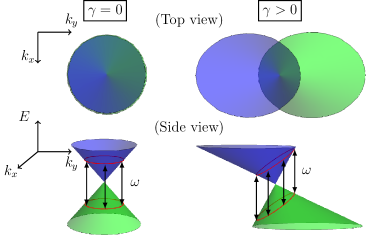
Figure 1: Comparison of a graphene-like dispersion with a tilted energy dispersion. Direct interband transitions on a tilted dispersion cone for a given constant frequency $\omega$ of the electric field arise from a non-isoenergetic curve, in contrast to transitions in a non-tilted dispersion.

In many 2D systems as in 8-Pmmn borophene, around one of the Dirac points, the low-energy excitations are described by an effective anisotropic tilted Dirac Hamiltonian of the form [28]

$$H=v_{x}\sigma_{x}k_{x}+v_{y}\sigma_{y}k_{y}+v_{t}\sigma_{0}k_{y}.$$ (1)

Here all energies are in units of $\hbar$. The other valley is studied through changing the sign of two velocities [28].

As seen in Fig. 1, the last term in Eq. (1) with nonzero $v_{t}$ produces a tilting of the dispersion cone in the $y$ direction. Also, as $v_{x}\neq v_{y}$ and $v_{t}\neq 0$, the cone’s constant energy contours are found to be elliptical rather than circular as in the particular case of graphene, for which $v_{x}=v_{y}$ and $v_{t}=0$. These distortions of the dispersion cones of 8-Pmmn borophene are found to produce direction dependent terms and scaling factors in the conductivity, both absent in graphene.

Although there are now some works in which the zero-temperature conductivity in anisotropic tilted Dirac Hamiltonians is calculated through the Kubo formula [39, 40, 31, 41], not so much attention has been drawn to the role of a non-zero temperature, or to the fact that different results depend upon different physical and mathematical limits. This is well known in graphene’s optical [42, 43, 2] and electronic properties [42, 43, 44, 2]. For example, in the low-frequency limit, graphene’s optical conductivity depends upon the sample through self-doping, scattering, temperature and ripple effects [42, 2].

The aim of this work is precisely to further investigate all the previous effects in the conductivity when applied to anisotropic tilted Dirac Hamiltonians, and specially to 8-Pmmn borophene. In particular, we are interested in the physical understanding of anisotropy and tilting effects on the intra and inter band scattering, which as we will show here, are far from trivial.

The layout is the following: In section II we calculate the conductivity: in subsection II.1 the calculation is done along the direction parallel to the tilt axis, in subsection II.2 we calculate the conductivity in the direction perpendicular to the tilt axis and contrast with the results of subsection II.1. Then, in section III we analyze the different frequency, temperature and scattering limits, and the minimal conductivities obtained thereof, followed by the discussion of the results in section IV. Finally, the conclusions are given in subsection IV.1.

II Conductivity for the anisotropic tilted Dirac Hamiltonian

Let us calculate the conductivity for the Hamiltonian given by Eq. (1). As represented in Fig. 1, the eigenvalues of this Hamiltonian are given by $E_{\pm}(\bm{k})=v_{t}k_{y}\pm\sqrt{v_{x}^{2}k_{x}^{2}+v_{y}^{2}k_{y}^{2}}$ with eigenvectors

$$|\Psi_{+}(\bm{k})\rangle=\frac{1}{\sqrt{2}}\left(\begin{array}[]{ccc}1\\ +e^{i\theta}\end{array}\right),\;\;\;|\Psi_{-}(\bm{k})\rangle=\frac{1}{\sqrt{2}}\left(\begin{array}[]{ccc}1\\ -e^{i\theta}\end{array}\right)$$ (2)

with $\theta$ defined by $\cos\theta=k_{x}/|k|$ and $\sin\theta=k_{y}/|k|$. Our aim is to obtain an expression for the real part of the diagonal conductivity from the Kubo formula [45, 43],

$$\sigma_{\nu\nu}=\pi\frac{e^{2}}{\hslash} \int\text{Tr}\{[H,r_{\nu}]\delta(H-\epsilon-\omega)$$ (3)

$$\times[H,r_{\nu}]\delta(H-\epsilon)\}\frac{f_{\beta}(\epsilon+\omega)-f_{\beta}(\epsilon)}{\omega}d\epsilon$$

where $r_{\nu}$ is the position coordinate in the $\nu=x$ or $\nu=y$ direction, $f_{\beta}(\epsilon)=1/[1+exp(\beta\epsilon)]$ is the Fermi distribution with $\beta=1/k_{B}T$, $T$ being the temperature and $\delta(x)$ is the Dirac delta function of $x$. In the limit $\beta\rightarrow\infty$, after changing $\epsilon\rightarrow\epsilon-\omega/2$, we obtain,

$$\sigma_{\nu\nu}=-\pi\frac{e^{2}}{\hslash}\frac{1}{\omega} \int_{-\omega/2}^{\omega/2}\text{Tr}\{[H,r_{\nu}]\delta(H-\omega/2-\epsilon)$$ (4)

$$\times[H,r_{\nu}]\delta(H+\omega/2-\epsilon)\}d\epsilon$$

Since the current operator is given by $j_{\nu}=-ie[H,r_{\nu}]$, the trace in Eq. (4) can be expressed as,

$$T(\epsilon)=\int\text{Tr}_{2}\biggl{[}\frac{\partial H}{\partial k_{\nu}} \delta(H-\omega/2-\epsilon)$$ (5)

$$\times\frac{\partial H}{\partial k_{\nu}}\delta(H+\omega/2-\epsilon)\biggr{]}\frac{d^{2}k}{(2\pi)^{2}},$$

where $\text{Tr}_{2}$ is the trace taken over the pseudospin degree of freedom. In order to investigate the effects introduced by the anisotropy on the electronic properties of this Hamiltonian, we calculate the components of the real conductivity in the direction of the tilt ($\sigma_{yy}$), and in the direction perpendicular to the tilt ($\sigma_{xx}$). These two cases are considered in the following subsections. Notice that for simplicity, here we start considering only one valley and spin. To find the total conductivity, on needs to take into account the corresponding factors, as we do in Section IV.

II.1 Conductivity in the direction parallel to the tilt

To obtain $\sigma_{yy}$, we start by writing the current operator in the $y$ direction,

$$j_{y}=-ie[H,y]\;\;\rightarrow\;\;e\frac{\partial H}{\partial k_{y}}=e\left(\begin{array}[]{ccc}v_{t}&-iv_{y}\\ iv_{y}&v_{t}\end{array}\right)$$ (6)

In order to evaluate the trace in Eq. (3), we rewrite $j_{y}$ in the $\{|\Psi_{+}\rangle,|\Psi_{-}\rangle\}$ basis. It reads,

$$j_{y}=\mathcal{U}\Big{(}e\frac{\partial H}{\partial k_{y}}\Big{)}\mathcal{U}^{\dagger}=ev_{y}\left(\begin{array}[]{ccc}\gamma+\sin\theta&i\cos\theta\\ -i\cos\theta&\gamma-\sin\theta\end{array}\right).$$ (7)

To simplify the calculation, we next propose a transformation which defines scaled momentums in such a way that the anisotropy due to $v_{x}$ and $v_{y}$ can be eliminated. Thus we define $\xi_{x}=v_{x}k_{x}$, $\xi_{y}=v_{y}k_{y}$, $\xi=\sqrt{\xi^{2}_{x}+\xi^{2}_{y}}$ and $\gamma=v_{t}/v_{y}$. Using these new variables, the Hamiltonian is written as,

$$H=\left(\begin{array}[]{ccc}\gamma\xi_{y}&\xi_{x}-i\xi_{y}\\ \xi_{x}+i\xi_{y}&\gamma\xi_{y}\end{array}\right),$$ (8)

Here $\gamma$ serves as a measure of the tilt in the dispersion cone, which in the present Hamiltonian occurs in the $y$ direction. The energy dispersion is now,

$$E_{\pm}(\bm{k})=\gamma\xi_{y}\pm\xi=(\gamma\sin\theta\pm 1)\xi.$$ (9)

where $\xi_{y}=\xi\sin\theta$ is in polar coordinates. Next we calculate $T(\epsilon)$ using Eq. (5), and as we show in Appendix A, for $\nu=y$ we obtain that

$$T( \epsilon)=\int\biggl{\{}\frac{(v_{t}\xi+v_{y}\xi_{y})^{2}}{\xi^{2}}\delta(\xi+\gamma\xi_{y}-\bar{\epsilon}_{+})\delta(\xi+\gamma\xi_{y}+\bar{\epsilon}_{-})+\frac{v_{y}^{2}\xi_{x}^{2}}{\xi^{2}}\delta(\xi-\gamma\xi_{y}+\bar{\epsilon}_{+})\delta(\xi+\gamma\xi_{y}+\bar{\epsilon}_{-})$$ (10)

$$+\frac{v_{y}^{2}\xi_{x}^{2}}{\xi^{2}}\delta(\xi+\gamma\xi_{y}-\bar{\epsilon}_{+})\delta(\xi-\gamma\xi_{y}-\bar{\epsilon}_{-})+\frac{(v_{t}\xi-v_{y}\xi_{y})^{2}}{\xi^{2}}\delta(\xi-\gamma\xi_{y}+\bar{\epsilon}_{+})\delta(\xi-\gamma\xi_{y}-\bar{\epsilon}_{-})\biggr{\}}\frac{d\xi_{x}d\xi_{y}}{v_{x}v_{y}(2\pi)^{2}},$$

where $\bar{\epsilon}_{\pm}=\omega/2\pm\epsilon$. This equation reduces to the case of graphene [43] for $\gamma=0$ and $v_{x}=v_{y}$. However, as a consequence of the tilting ($\gamma\neq 0$), $T(\epsilon)$ is no longer symmetric under $\epsilon\rightarrow-\epsilon$, rather, it is symmetric under $\epsilon\rightarrow-\epsilon$, $\xi_{y}\rightarrow-\xi_{y}$.

We denote the terms in the above integral as $T(\epsilon)=T_{+}^{tra}(\epsilon)+T_{+}^{ter}(\epsilon)+T_{-}^{ter}(\epsilon)+T_{-}^{tra}(\epsilon)$. The superscript $tra$ is used to denote intraband contributions while the superscript $ter$ denotes interband contributions. The first term of the previous equation, in polar coordinates reads

$$T_{+}^{tra}(\epsilon)=\int_{0}^{2\pi} \int_{0}^{\lambda}\frac{v_{y}}{v_{x}}(\gamma+\sin\theta)^{2}\delta(\xi(1+\gamma\sin\theta)-\bar{\epsilon}_{+})$$ (11)

$$\times\delta(\xi(1+\gamma\sin\theta)+\bar{\epsilon}_{-})\frac{\xi d\xi d\theta}{(2\pi)^{2}}$$

after using $\xi_{y}=\xi\sin\theta$, $\gamma=v_{t}/v_{y}$ and $d\xi_{x}d\xi_{y}\rightarrow\xi d\xi d\theta$, and having introduced $\lambda$ as a high energy cutoff [43]. Similar definitions are used for the other three terms $T_{+}^{ter}(\epsilon),T_{-}^{ter}(\epsilon),T_{-}^{tra}(\epsilon)$. We introduce a scattering rate $\eta$ by considering soft Dirac delta functions $\delta_{\eta}(x)$

$$\delta(x)\approx\delta_{\eta}(x)=\lim_{\eta\rightarrow 0}\frac{1}{\pi}\frac{\eta}{x^{2}+\eta^{2}}.$$ (12)

As we will integrate over $\xi$ before $\theta$, we define $\gamma_{+}=1+\gamma\sin\theta$ and then express the first Dirac delta in Eq. (11) as

$$\delta_{\eta}(\gamma_{+}\xi-\bar{\epsilon}_{+})=\frac{1}{\gamma_{+}}\delta_{\eta_{+}}\Big{(}\xi-\frac{\bar{\epsilon}_{+}}{\gamma_{+}}\Big{)}$$ (13)

with $\eta_{+}=\eta/\gamma_{+}$. For these and further equations to remain well defined we will assume that $0\leq\gamma<1$, which in the three dimensional case defines a type-I Weyl semimetal [46, 3].

We will further make the assumption that $\gamma$ does not take values too close to unity so $\eta_{\pm}\rightarrow 0$ remains valid. This means that $\delta_{\eta_{\pm}}(x)$ stays as a good approximation to a (soft) Dirac delta function so we can consider $\delta_{\eta_{\pm}}(x)\approx\delta_{\eta}(x)$, by taking $\gamma\eta\rightarrow 0$.

After having defined $\gamma_{-}=1-\gamma\sin\theta$, $\eta_{-}=\eta/\gamma_{-}$, and expressing the delta functions as in Eq. (13), the four terms in the trace in Eq. (10) can be divided into two intraband contributions,

$$T_{\pm}^{tra}(\epsilon)=\int_{0}^{2\pi}\int_{0}^{\lambda}g_{\pm}(\theta)\delta_{\eta}\Big{(}\xi\mp\frac{\bar{\epsilon}_{+}}{\gamma_{\pm}}\Big{)}\delta_{\eta}\Big{(}\xi\pm\frac{\bar{\epsilon}_{-}}{\gamma_{\pm}}\Big{)}\frac{\xi d\xi d\theta}{(2\pi)^{2}},$$ (14)

and two interband contributions,

$$T_{\pm}^{ter}(\epsilon)=\int_{0}^{2\pi}\int_{0}^{\lambda}l(\theta)\delta_{\eta}\Big{(}\xi\pm\frac{\bar{\epsilon}_{+}}{\gamma_{\mp}}\Big{)}\delta_{\eta}\Big{(}\xi\pm\frac{\bar{\epsilon}_{-}}{\gamma_{\pm}}\Big{)}\frac{\xi d\xi d\theta}{(2\pi)^{2}},$$ (15)

where,

$$g_{\pm}(\theta)=\frac{v_{y}}{v_{x}}(\gamma\pm\sin\theta)^{2}\frac{1}{\gamma_{\pm}^{2}}$$ (16)

and,

$$l(\theta)=\frac{v_{y}}{v_{x}}\frac{\cos^{2}\theta}{\gamma_{+}\gamma_{-}}$$ (17)

The radial integrals in eqs. (14-15) involving the product of soft Dirac delta functions can be expressed as

$$\int_{0}^{\lambda} \delta_{\eta}(\xi-a)\delta_{\eta}(\xi-b)\xi d\xi\sim(a+b)\delta_{\eta}\left(a-b\right)\frac{1}{4}[\Theta(\lambda-a)$$ (18)

$$+\Theta(a)+\Theta(\lambda-b)+\Theta(b)-2]-\frac{\eta}{a-b}\frac{1}{2\pi}[\Theta(\lambda-b)$$

$$+\Theta(b)-\Theta(\lambda-a)-\Theta(a)].$$

Evaluation of the radial integrals and addition of the four trace terms of Eq. (10) (see Appendix A) leads to,

$$T (\epsilon)=\frac{v_{y}}{v_{x}}\frac{\pi}{(2\pi)^{2}}\Biggl{\{}\int_{0}^{2\pi}\frac{\cos^{2}\theta}{1-\gamma^{2}\sin^{2}\theta}\Bigl{(}\frac{\omega}{4}-\frac{\epsilon}{2}\gamma\sin\theta\Bigr{)}$$ (19)

$$\times\delta_{\eta}\Bigl{(}\epsilon-\frac{\omega}{2}\gamma\sin\theta\Bigr{)}\frac{d\theta}{\pi}+\frac{\eta}{\pi\omega}\varphi_{yy}^{tra}(\gamma)\Biggr{\}}\Theta\Bigl{(}\lambda-\frac{\omega}{2}\Bigr{)}.$$

The first term in $T(\epsilon)$ is related to interband scattering, while the second term describes intraband scattering. An overall scaling factor of $v_{y}/v_{x}$ is introduced due to the anisotropy, and the function $\varphi_{yy}^{tra}(\gamma)$ enhances the intraband term as a consequence of the tilt in the energy dispersion. It is given by,

$$\varphi^{tra}_{yy}(\gamma)=\frac{2}{\gamma^{2}}[(1-\gamma^{2})(\sqrt{1-\gamma^{2}}-1)+\gamma^{2}].$$ (20)

We plot $\varphi^{tra}_{yy}(\gamma)$ in Fig. 2. The magnitude of the intraband scattering term increases with the tilt; it reduces to that of graphene for $\gamma=0$. For the case of Pmmn-8 borophene [28], $\gamma=0.46$, resulting in $\varphi^{tra}_{yy}(\gamma)\approx 1.16$.

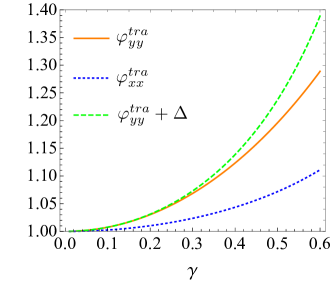
Figure 2: A comparison of the different adimensional factors that appear in the conductivity due to the tilt strength $\gamma\neq 0$ of the energy dispersion. When a tilt is introduced in the $y$ direction, $\varphi^{tra}_{yy}(\gamma)$ enters the intraband contribution of $\sigma_{yy}$, while $\varphi^{tra}_{xx}(\gamma)$ enters the intraband contribution of $\sigma_{xx}$. The factor $\varphi_{yy}^{tra}+\Delta$ enters the minimal conductivity of Eq. (32). All of these factors reduce to unity for a dispersion with no tilt.

We can now calculate the temperature dependent conductivity by substituting Eq. (19) into Eq. (3) (see Appendix B).

Finally, we obtain that for $\omega<2\lambda$,

$$\sigma_{yy} \sim\frac{v_{y}}{v_{x}}\Biggl{\{}\varphi_{yy}^{ter}(\gamma,\beta\omega)\frac{\pi e^{2}}{8h}\tanh\Bigg{(}\frac{\beta\omega}{4}\Bigg{)}$$ (21)

$$+\varphi_{yy}^{tra}(\gamma)\frac{e^{2}}{h}\frac{\beta\eta}{(\beta\omega)^{2}}\log\Biggl{[}\frac{1+\tanh^{2}(\beta\omega/4)}{1-\tanh^{2}(\beta\omega/4)}\Biggr{]}\Biggr{\}}$$

and the conductivity vanishes for $\omega>2\lambda$. Notice that in the previous equation we defined the interband scattering factor as,

$$\tanh\Bigg{(}\frac{\beta\omega}{4}\Bigg{)}\varphi_{yy}^{ter}(\gamma,\beta\omega)=$$

$$\int_{0}^{2\pi}\cos^{2}\theta\frac{\sinh(\beta\omega/2)}{\cosh(\beta\omega/2)+\cosh(\beta\frac{\omega}{2}\gamma\sin\theta)}\frac{d\theta}{\pi}$$ (22)

After taking an expansion in $\gamma$, we obtain

$$\varphi_{yy}^{ter}(\gamma,\beta\omega)=1-\frac{\gamma^{2}}{4}\left(\frac{\beta\omega}{4}\right)^{2}\text{Sech}^{2}\Bigg{(}\frac{\beta\omega}{4}\Bigg{)}+O(\gamma)^{4}$$ (23)

For $\gamma=0$ we recover the case of graphene, as $\varphi_{yy}^{ter}=1$. However, unlike in the intraband scattering factor, $\varphi_{yy}^{ter}$ is not only a function of $\gamma$, but of $\beta\omega$ as well.

The tilting has no effect in the interband conductivity in the limits $\beta\omega\rightarrow 0$ and $\beta\omega\rightarrow\infty$, as in both cases $\varphi_{yy}^{ter}(\gamma,\beta\omega)=1$, just as in the case of no tilt ($\gamma=0$). For finite values of $\beta\omega$, $\varphi_{yy}^{ter}$ decreases with $\gamma$ in contrast to $\varphi_{yy}^{tra}(\gamma)$, which monotonically increases.

In Fig. 3 we present the resulting $\sigma_{yy}$ (and also $\sigma_{xx}$, see next section for details on the calculation) as a function of $\beta\omega$ for the case of 8-Pmmn borophene using two different values for the scattering, $\beta\eta=1$ and $\beta\eta=4$. For comparison proposes, we also plot graphene’s conductivity. The predicted conductivity for 8-Pmmn borophene is smaller than that of graphene in the tilt direction, and larger in the perpendicular direction. In this case, the scaling factors $v_{\mu}/v_{\nu}$ dominate over the tilt factors $\varphi_{\mu\mu}^{intra}$ and $\varphi_{\mu\mu}^{inter}$. In order to show the effect introduced purely by the tilt, in Fig. 4 is shown a comparison between graphene’s conductivity and the geometric average $\langle\sigma\rangle=\sqrt{\sigma_{xx}\sigma_{yy}}$ for borophene, which is independent of $v_{x}$ and $v_{y}$. We can see that for the high-frequency limit, the mean geometrical conductivity is the same as in graphene.

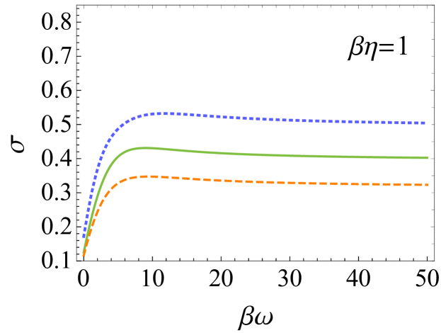
(a)

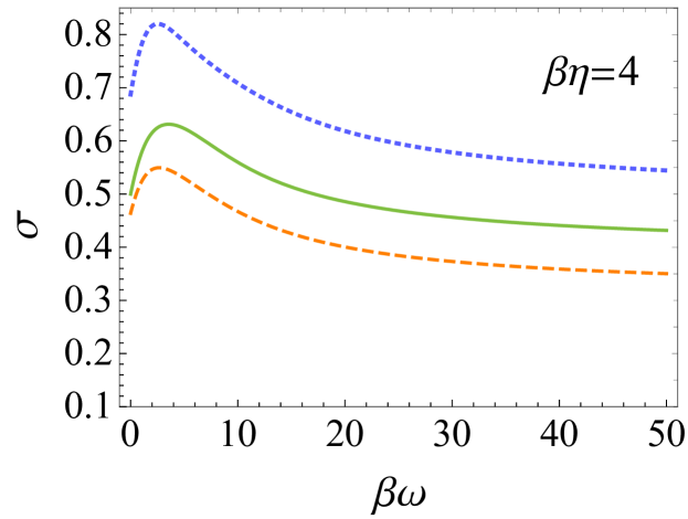
(b)

Figure 3: Conductivity of 8-Pmmn borophene in the tilt axis $\sigma_{yy}$ (dashed curves), and the perpendicular axis $\sigma_{xx}$ (dotted curves), compared to that of graphene (solid curves) for the constant rates (a) $\beta\eta=1$ and (b) $\beta\eta=4$ assumed constant. Notice the anisotropy with respect to graphene. In the low-frequency limit for a fixed $T$, the conductivity depends upon the scattering. In the high-frequency region, it reaches the same limit for different amounts of scattering as happens with graphene. The numerical values for $v_{x}$, $v_{y}$ and $v_{t}$ were taken from [28].

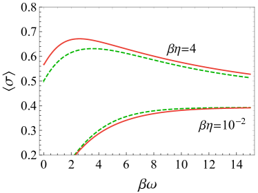
Figure 4: Comparison of graphene’s conductivity (dashed lines) vs the geometric mean $\langle\sigma\rangle=\sqrt{\sigma_{xx}\sigma_{yy}}$ of 8-Pmmn borophene (solid lines) at different scattering rates $\beta\eta=10^{-2}$ (lower curves) and $\beta\eta=4$ (upper curves).

As in graphene, samples under typical experimental situations have an appreciable spontaneous doping which is able to reduce the transition strength due to state blocking [42]. This can be accounted for by introducing a nonzero chemical potential $\mu$ relative to the Dirac point, which essentially shifts the peak of $\sigma$, giving a vanishing conductivity for values of $\omega<2\mu$ and having practically no effect when $\omega>2\mu$ [42, 31].

Notice that apart from $\varphi_{yy}^{ter}$ and $\varphi_{yy}^{tra}$, the anisotropy in the energy dispersion introduces an additional scaling factor $v_{y}/v_{x}$ to $\sigma_{yy}$, in agreement with calculations using the Landauer formalism [38] or in a semi-Dirac material [47].

II.2 Conductivity in the direction perpendicular to the tilt

The calculation of $\sigma_{xx}$ can be performed by following the same steps as those presented in the previous section. The result is,

$$\sigma_{xx} \sim\frac{v_{x}}{v_{y}}\Biggl{\{}\varphi_{xx}^{ter}(\gamma,\beta\omega)\frac{\pi e^{2}}{8h}\tanh\Biggl{(}\frac{\beta\omega}{4}\Biggr{)}$$ (24)

$$+\varphi_{xx}^{tra}(\gamma)\frac{e^{2}}{h}\frac{\beta\eta}{(\beta\omega)^{2}}\log\Biggl{[}\frac{1+\tanh^{2}(\beta\omega/4)}{1-\tanh^{2}(\beta\omega/4)}\Biggr{]}\Biggr{\}}$$

The intraband scattering factor is,

$$\varphi_{xx}^{tra}(\gamma)=\int_{0}^{2\pi}\frac{1}{2\pi}\bigg{\{}\frac{\cos^{2}\theta}{\gamma_{+}}+\frac{\cos^{2}\theta}{\gamma_{-}}\bigg{\}}d\theta=\frac{2}{\gamma^{2}}[1-\sqrt{1-\gamma^{2}}]$$ (25)

This function is analogous to $\varphi_{yy}^{tra}$; it also grows from unity as $\gamma$ increases, but it takes lower values. Both $\varphi_{xx}^{tra}$ and $\varphi_{yy}^{tra}$ are compared in Fig. 2.

The interband scattering factor is given by,

$$\varphi_{xx}^{ter}(\gamma,\beta\omega)=1-\frac{3\gamma^{2}}{4}\left(\frac{\beta\omega}{4}\right)^{2}\text{Sech}^{2}\Bigg{(}\frac{\beta\omega}{4}\Bigg{)}+O(\gamma)^{4}$$ (26)

It is worthwhile to remark that our Eqs. (21) and (24) generalize Eq. (13) of Ref. [43], to which our expressions reduce for $v_{y}=v_{x}$ and $\gamma=0$.

III Minimal conductivity

In graphene, it is known that the minimal conductivity approaches different limits depending upon the scattering, frequency and temperature [42, 43]. In this section, we explore such limits.

III.1 Zero temperature

We put Eq. (19) into the conductivity of Eq. (4) and obtain

$$\sigma_{yy}=\frac{v_{y}}{v_{x}}\frac{\pi}{8}\Bigg{(}1+\frac{4\eta}{\pi\omega}\varphi_{yy}^{tra}(\gamma)\Bigg{)}\frac{e^{2}}{h},$$ (27)

Evaluating the limits discussed by Ziegler in Ref. [43] at temperature zero we obtain,

$$\sigma_{yy,1}^{min}=\frac{v_{y}}{v_{x}}\varphi_{xx}^{tra}(\gamma)\frac{1}{\pi}\frac{e^{2}}{h},$$ (28)

taking $\omega\rightarrow 0$ in Eq. (10) then $\eta\rightarrow 0$,

$$\sigma_{yy,2}^{min}=\frac{v_{y}}{v_{x}}\frac{\pi}{8}\frac{e^{2}}{h}\qquad\text{for {\hbox{\eta\approx 0}}},$$ (29)

$$\sigma_{yy,3}^{min}=\frac{v_{y}}{v_{x}}\frac{\pi}{4}\bigg{(}\frac{1+\varphi_{yy}^{tra}(\gamma)}{2}\bigg{)}\frac{e^{2}}{h}\qquad\text{for {\hbox{\eta\approx\omega}}},$$ (30)

these are to be compared to eqs. (15-17) of [43]. The intraband factor that appears in the expression for $\sigma_{xx}$ enters $\sigma_{yy,1}^{min}$ and, while the minimal conductivities in eqs. (28) and (30) increase with the tilt, the one in Eq. (29) is not affected by it.

Quite analogous, for the zero temperature $\sigma_{xx}$ we obtain

$$\sigma_{xx}=\frac{v_{x}}{v_{y}}\frac{\pi}{8}\Bigg{(}1+\frac{4\eta}{\pi\omega}\varphi_{xx}^{tra}(\gamma)\Bigg{)}\frac{e^{2}}{h},$$ (31)

$$\sigma_{xx,1}^{min}=\frac{v_{x}}{v_{y}}[\varphi_{yy}^{tra}(\gamma)+\Delta(\gamma)]\frac{1}{\pi}\frac{e^{2}}{h}$$ (32)

taking $\omega\rightarrow 0$ in Eq. (10) then $\eta\rightarrow 0$,

$$\sigma_{xx,2}^{min}=\frac{v_{x}}{v_{y}}\frac{\pi}{8}\frac{e^{2}}{h}\qquad\text{for {\hbox{\eta\approx 0}}},$$ (33)

$$\sigma_{xx,3}^{min}=\frac{v_{x}}{v_{y}}\frac{\pi}{4}\bigg{(}\frac{1+\varphi_{xx}^{tra}(\gamma)}{2}\bigg{)}\frac{e^{2}}{h}\qquad\text{for {\hbox{\eta\approx\omega}}},$$ (34)

having introduced $\Delta(\gamma)$ such that $\varphi_{yy}^{tra}(\gamma)+\Delta(\gamma)=2[(1-\gamma^{2})^{-1/2}-1]/\gamma^{2}$. These values are plotted and compared in Fig. 2. We note that for small values of $\gamma$, $\Delta(\gamma)\approx 0$ and then all of eqs. (31-34) are symmetrical to eqs. (27-30) under the interchange $\varphi_{xx}^{tra}\leftrightarrow\varphi_{yy}^{tra}$ and $v_{y}/v_{x}\leftrightarrow v_{x}/v_{y}$.

III.2 Frequency and temperature dependence

Now, considering the asymptotic regimes $\beta\omega\rightarrow 0$ and $\beta\omega\rightarrow\infty$ for the conductivity in Eq. (21) leads to

$$\sigma_{yy}^{\prime}\sim\frac{v_{y}}{v_{x}}\frac{e^{2}}{8h}\Bigg{\{}\begin{array}[]{cc}\text{$\;\,\varphi_{yy}^{tra}(\gamma)\times\beta\eta$ \qquad\qquad for $\beta\omega\sim 0$},\\ \text{$\pi+\varphi_{yy}^{tra}(\gamma)\times 4\beta\eta/\beta\omega$ \quad for $\beta\omega\sim\infty$}.\end{array}$$ (35)

Similarly, for the conductivity in Eq. (24),

$$\sigma_{xx}^{\prime}\sim\frac{v_{x}}{v_{y}}\frac{e^{2}}{8h}\Bigg{\{}\begin{array}[]{cc}\text{$\;\,\varphi_{xx}^{tra}(\gamma)\times\beta\eta$ \qquad\qquad for $\beta\omega\sim 0$},\\ \text{$\pi+\varphi_{xx}^{tra}(\gamma)\times 4\beta\eta/\beta\omega$ \quad for $\beta\omega\sim\infty$}.\end{array}$$ (36)

IV Discussion of the results

We first discuss our results in the zero temperature, dc limit. The minimal conductivities in Eqs. (28) and (32) can be written as

$$\sigma_{yy,1}^{min}=\frac{v_{y}}{v_{x}}\frac{1}{\pi}\frac{e^{2}}{h}\frac{2}{\gamma^{2}}\left(\frac{1}{\sqrt{1-\gamma^{2}}}-1\right)\sqrt{1-\gamma^{2}}$$ (37)

$$\sigma_{xx,1}^{min}=\frac{v_{x}}{v_{y}}\frac{1}{\pi}\frac{e^{2}}{h}\frac{2}{\gamma^{2}}\left(\frac{1}{\sqrt{1-\gamma^{2}}}-1\right).$$ (38)

We notice that both $\sigma_{xx,1}^{min}$ and $\sigma_{yy,1}^{min}$ increase with the tilt parameter $\gamma$, while $\sigma_{xx,1}^{min}>\sigma_{yy,1}^{min}$ and only $\sigma_{xx,1}^{min}$ diverges as $\gamma\rightarrow 1$ [39, 41]. This limit coincides with recent calculations of the static conductivity using the covariant Boltzmann equation [41]. The fact that both $\sigma_{xx,1}^{min}$ and $\sigma_{yy,1}^{min}$ grow with the tilt of the dispersion can be attributed to the increase in the density of states with the tilt parameter $\gamma$,

$$\rho(E)=\sum_{\bm{k}}^{|k|<k_{F}}\delta(E_{\pm}(\bm{k})-E)=\frac{|E|}{2\pi v_{x}v_{y}}(1-\gamma^{2})^{-3/2}$$ (39)

To account for the anisotropy we point out that the constant-energy cross sections of the dispersion cone describe ellipses in momentum space given by $(v_{x}k_{x})^{2}/A^{2}+(v_{y}k_{y}-h)^{2}/B^{2}=1$ with $h=\pm\gamma E/(1-\gamma^{2})$, $A=E/\sqrt{1-\gamma^{2}}$ and $B=E/(1-\gamma^{2})$. As the tilt increases, the eccentricity of the isoenergetic ellipses becomes more pronounced and scattering events across the shorter axis (here the x-axis) become more probable [41, 39] than along the tilt axis (here the y-axis). We further note that in the purely tilted case ($v_{x}=v_{y}$) the ratio between the lengths of the ellipse’s semi-axes $B/A$ is precisely equal to the ratio between these conductivities

$$\frac{\sigma_{xx,1}^{min}}{\sigma_{yy,1}^{min}}=\frac{1}{\sqrt{1-\gamma^{2}}}=\frac{B}{A}.$$ (40)

When anisotropy ($v_{y}\neq v_{x}$) is introduced, we obtain a direction-dependent scaling of the components $\sigma_{\nu\nu}$ of the form $v_{\nu}/v_{\mu}$ which is in agreement with calculations using the Landauer formalism [38] or in a semi-Dirac material [47].

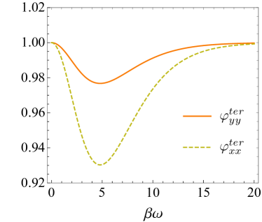
Figure 5: Comparison of the adimensional factors that appear in the interband components of the conductivity due to a tilt strength $\gamma=0.46$ which has been reported for 8-Pmmn borophene’s energy dispersion [28]. $\varphi_{xx}^{ter}$ enters the interband component of $\sigma_{xx}$ and $\varphi_{yy}^{ter}$ enters the interband component of $\sigma_{yy}$. A minimum is observed for $\beta\omega\approx 4$ for any $\gamma\neq 0$.

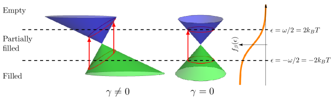
Figure 6: Comparison of interband transitions occurring in a material with a tilted ($\gamma\neq 0$) vs a non-tilted ($\gamma=0$) dispersion cone when $\beta\omega\approx 4$. The red contours in the cones indicate the states the can participate in direct interband transitions i.e., states that satisfy $E_{+}(\bm{k})-E_{-}(\bm{k})=\omega$. When $\gamma\neq 0$, the contours tilt and half of their perimeter lays in the partially-filled energy region, where the total number of states available for transitions decreases. This reduces the interband conductivity around $\beta\omega\approx 4.$

Our results show that in the zero temperature limit interband transitions are not affected by the tilt in the dispersion. As shown in Fig. 6, such results comes out from the global tilting of the transitions. This can also be readily verified by using the Fermi golden rule, i.e., we introduce the electric field $\bm{E}$ as a perturbation $\delta H$ to the Hamiltonian in Eq. (1) as

$$H=\bm{\sigma}^{\prime}\cdot(\bm{p}-\frac{e}{c}\bm{A})\equiv H_{0}+\delta H$$ (41)

where $\bm{\sigma}^{\prime}=(v_{x}\sigma_{x},v_{y}(\sigma_{y}+\gamma\sigma_{0}))/\hbar$, $\bm{p}=\hbar\bm{k}$ and $\partial\bm{A}/\partial t=-c\bm{E}$. The perturbation is then given by [48]

$$\delta H=\frac{ie}{2\omega}\bm{\sigma}^{\prime}\cdot\bm{E}$$ (42)

According to the Fermi golden rule, the absorption energy per unit time for direct interband transitions $E_{-}(\bm{k})\rightarrow E_{+}(\bm{k})$ between states with an energy difference $\Delta E=\omega$ is [48, 49]

$$W=g_{d}\sum_{\bm{k}}4\pi\omega|\langle\Psi_{+}(\bm{k})|\delta H|\Psi_{-}(\bm{k})\rangle|^{2}\delta(E_{+}(\bm{k})-E_{-}(\bm{k})-\omega)$$ (43)

where $g_{d}=4$ takes into account valley and spin degeneracy. It can be easily seen that the transition amplitude $\langle\Psi_{+}(\bm{k})|\delta H|\Psi_{-}(\bm{k})\rangle$ is independent of $\gamma$, as the term proportional to $\sigma_{0}$ is eliminated due to the orthogonal character of the basis. Moreover, we make the observation that the density of states implied in Eq. (43) is not the same as the one in Eq. (39). This is due to the tilt, as the states that participate in interband transitions between states with a given energy difference $\Delta E=\omega$ do not lay on an isoenergetic curve in the dispersion (Fig. 1), unlike in graphene ($\gamma=0$), where the density of states that enters the expression for the transition rate is simply $\rho(\omega/2)$. Rather, the density of final states for direct interband transitions with $\Delta E=\omega$ is given by (see Appendix C)

$$D(\omega/2)\equiv 2g_{d}\sum_{\bm{k}}\delta(E_{+}(\bm{k})-E_{-}(\bm{k})-\omega)=\frac{\omega}{\pi v_{x}v_{y}}$$ (44)

which is independent of $\gamma$. In the isotropic case ($v_{x}=v_{y}$), $D(\omega/2)$ is exactly graphene’s density of final states $\rho(\omega/2)$ for interband transitions with $\Delta E=\omega$.

The final expressions for the absorption coefficient on each direction are

$$\frac{W_{x}}{W_{i}}=\frac{v_{x}}{v_{y}}\frac{\pi e^{2}}{\hbar c},\quad\frac{W_{y}}{W_{i}}=\frac{v_{y}}{v_{x}}\frac{\pi e^{2}}{\hbar c}$$ (45)

where $W_{i}=c|\bm{E}|/4\pi\hbar$ is the incident energy flux [48]. When $v_{x}=v_{y}$, this direction-dependent optical absorption coefficient reduces to the isotropic constant value of $\pi e^{2}/\hbar c=\pi\alpha$ measured in graphene [42, 50]. This shows that in the $T\rightarrow 0$ limit, the tilt in the dispersion has no effect on interband transitions, a fact consistent with the expressions for the factors $\varphi_{\mu\mu}^{ter}$ obtained from the Kubo formula (Fig. 5). Notice that for intraband transitions, the relevant density of states is that in Eq. (39), while for analyzing the interband transitions, the $\gamma$-independent density of states in Eq. (44) should be used. The former is related to the states in a isoenergetic cross-section of the dispersion (which is to be taken into account in elastic scattering events) and the latter is related to the states that can participate in direct interband transitions.

Thus, our results show that the intraband contribution to the conductivity, which is related to the Drude peak, is enhanced by the tilt in the energy dispersion, and this effect is highly anisotropical.

On the other hand, for the interband conductivity we obtain that both components $\sigma_{yy}$ and $\sigma_{xx}$ decrease in the limit where $\beta\omega$ takes a finte value. Moreover, if we express Eq. (26) as $\varphi_{xx}^{ter}=1-\delta\varphi_{xx}^{ter}$, and do similarly for $\varphi_{yy}^{ter}$, comparing this equation with Eq. (23), we note that,

$$\delta\varphi_{xx}^{ter}+\delta\varphi_{yy}^{ter}=\gamma^{2}c_{v}/k_{B}$$ (46)

up to $O(\gamma)^{4}$ terms, where $c_{v}$ is the heat capacity (per particle) of a two level system with an energy gap of $\Delta E=\omega/2$,

$$c_{v}=k_{B}\left(\frac{\beta\Delta E}{2}\right)^{2}\text{Sech}^{2}\left(\frac{\beta\Delta E}{2}\right)$$ (47)

In Fig. 5, we present the resulting curves for $\varphi_{xx}^{ter}$ and $\varphi_{yy}^{ter}$. Notice that as happens with the specific heat of a two-level system, there is a maximum for $c_{v}$ which in this case results in a minimum for $\varphi_{xx}^{ter}$ and $\varphi_{yy}^{ter}$ as a function of $\beta\omega$. This occurs at $\beta\omega\approx 4$ as obtained from the derivative of Eq. (47). A sketch of its explanation is presented in Fig. 6. The minimum arises as an interplay between the partially-filled energy region in the Fermi distribution, which extends approximately from $-2k_{B}T$ to $+2k_{B}T$ around the chemical potential, with the tilted cross-sections in the cone that carry interband transitions for a given $\omega$ . In the case of graphene ($\gamma=0$), the interband conductivity takes a constant value for $\beta\omega\gtrsim 4$ and it starts to decrease when $\beta\omega\lesssim 4$ [43], as the contours in the dispersion cone that participate in interband transitions start to enter the partially-filled energy region, where the number of total states available for transitions is reduced. When $\gamma\neq 0$, as in 8-Pmmn borophene, these contours are tilted and as a result, when $\beta\omega\approx 4$, already half of their perimeter is in the region of partially filled states. This accounts for the reduction of the mean geometrical conductivity of 8-Pmmn borophene with respect to that of graphene in a wide range around $\beta\omega\approx 4$ shown in Fig. 4 for $\beta\eta=10^{-2}$.

IV.1 Conclusions

We have investigated the temperature-dependent optical conductivity of anisotropic tilted Dirac semimetals using the Kubo formula and discussed our results in the context of 8-Pmmn borophene. The effects of the tilting on interband and intraband scattering were analyzed in detail. We found direction-dependent scaling factors that appear due to the anisotropy of the energy dispersion and an anisotropic increase of the intraband conductivity with the tilt strength $\gamma$, which can be attributed to the deformation of the constant-energy contours of the dispersion cone into ellipses. In the zero-temperature, dc limit, our results are in agreement with recent calculations of the static conductivity using the covariant Boltzmann equation [41]. We also found most of the limits leading to minimal conductivities that increase with the tilt strength. Our results reproduce those of graphene reported in [43] for the particular case of an isotropic energy dispersion with no tilt. Moreover, the conductivity is similar to that found in graphene but weighted by the anisotropy in such a way that the mean geometrical conductivity is the same as in graphene for the high frequency or low temperature limit. This is a consequence of the fact that in such limit, interband transitions are not affected by the tilt in the dispersion, a result that was verified by a direct use of the Fermi golden rule. Finally, as the temperature was raised, a minimum of the interband dispersion was observed as a result of the interplay between tilting and the derivative of the Fermi distribution widening with temperature. Such minimum can be tested by a suitable optical experiment.

Appendix A Calculation of the trace factor $T(\epsilon)$ in the expression for $\sigma_{yy}$

In this section we calculate the trace factor in Eq. (4). For $\nu=y$ we have defined

$$T(\epsilon) =-\text{Tr}\{[H,r_{y}]\delta(H-\omega/2-\epsilon)[H,r_{y}]\delta(H+\omega/2-\epsilon)\}$$

$$=\int\text{Tr}_{2}\biggl{[}\frac{\partial H}{\partial k_{y}}\delta\bigl{(}H-\frac{\omega}{2}-\epsilon\bigr{)}\frac{\partial H}{\partial k_{y}}\delta\bigl{(}H+\frac{\omega}{2}-\epsilon\bigr{)}\biggr{]}\frac{d^{2}k}{(2\pi)^{2}}$$

Expanding the trace over the pseudospin degree of freedom we get

$$T(\epsilon) =\int\{\langle\Psi_{+}|\Lambda_{1}|\Psi_{+}\rangle\langle\Psi_{+}|\Lambda_{2}|\Psi_{+}\rangle$$ (48)

$$+\langle\Psi_{+}|\Lambda_{1}|\Psi_{-}\rangle\langle\Psi_{-}|\Lambda_{2}|\Psi_{+}\rangle+\langle\Psi_{-}|\Lambda_{1}|\Psi_{+}\rangle\langle\Psi_{+}|\Lambda_{2}|\Psi_{-}\rangle$$

$$+\langle\Psi_{-}|\Lambda_{1}|\Psi_{-}\rangle\langle\Psi_{-}|\Lambda_{2}|\Psi_{-}\rangle\}\frac{d^{2}k}{(2\pi)^{2}},$$

where we have defined the operators

$$\Lambda_{1}=\frac{\partial H}{\partial k_{y}}\delta(H-\frac{\omega}{2}-\epsilon),\;\;\;\Lambda_{2}=\frac{\partial H}{\partial k_{y}}\delta(H+\frac{\omega}{2}-\epsilon).$$

Substitution of the elements of the current operator in Eq. (7) into Eq. (48) leads to Eq. (10). In the following, we will assume $-\omega/2\leq\epsilon\leq\omega/2$, which is justified for low temperatures.

A.1 Expression for $T_{+}^{ter}(\epsilon)$

From Eq. (15),

$$T_{+}^{ter}(\epsilon)=\int_{0}^{2\pi}l(\theta)\int_{0}^{\lambda}\delta_{\eta}\Big{(}\xi+\frac{\bar{\epsilon}_{+}}{\gamma_{-}}\Big{)}\delta_{\eta}\Big{(}\xi+\frac{\bar{\epsilon}_{-}}{\gamma_{+}}\Big{)}\frac{\xi d\xi d\theta}{(2\pi)^{2}}.$$ (49)

Comparing with Eq. (18) we identify $a=-\bar{\epsilon}_{+}/\gamma_{-}$ and $b=-\bar{\epsilon}_{-}/\gamma_{+}$. As $a,b\leq 0$, we have $\Theta(a)=\Theta(b)=0$ and $\Theta(\lambda-a)=\Theta(\lambda-b)=1$. Therefore, according to Eq. (18), $T_{+}^{ter}(\epsilon)=0$.

A.2 Expression for $T_{-}^{ter}(\epsilon)$

From Eq. (15),

$$T_{-}^{ter}(\epsilon)=\int_{0}^{2\pi}\int_{0}^{\lambda}l(\theta)\delta_{\eta}\Big{(}\xi-\frac{\bar{\epsilon}_{+}}{\gamma_{+}}\Big{)}\delta_{\eta}\Big{(}\xi-\frac{\bar{\epsilon}_{-}}{\gamma_{-}}\Big{)}\frac{\xi d\xi d\theta}{(2\pi)^{2}}$$ (50)

Comparing to Eq. (18) we identify $a=\bar{\epsilon}_{+}/\gamma_{+}$ and $b=\bar{\epsilon}_{-}/\gamma_{-}$. As $a,b\geq 0$, we have $\Theta(a)=\Theta(b)=1$. Adding the inequalities $\lambda>a$ and $\lambda>b$ leads to $\Theta(\lambda-a)+\Theta(\lambda-b)=2\Theta(\lambda-\omega/2)$ and $\Theta(\lambda-a)-\Theta(\lambda-b)=0$. Therefore, according to Eq. (18),

$$T_{-}^{ter}(\epsilon)=\int_{0}^{2\pi}l(\theta)\Bigl{(}\frac{\omega}{4}-\frac{\epsilon}{2} \gamma\sin\theta\Bigr{)}\delta_{\eta}\Bigl{(}\epsilon-\frac{\omega}{2}\gamma\sin\theta\Bigr{)}$$ (51)

$$\times\frac{d\theta}{(2\pi)^{2}}\Theta(\lambda-\omega/2).$$

A.3 Expressions for $T_{+}^{tra}(\epsilon)$ and $T_{-}^{tra}(\epsilon)$

From Eq.(14),

$$T_{+}^{tra}(\epsilon)=\int_{0}^{2\pi}\int_{0}^{\lambda}g_{+}(\theta)\delta_{\eta}\Big{(}\xi-\frac{\bar{\epsilon}_{+}}{\gamma_{+}}\Big{)}\delta_{\eta}\Big{(}\xi+\frac{\bar{\epsilon}_{-}}{\gamma_{+}}\Big{)}\frac{\xi d\xi d\theta}{(2\pi)^{2}}.$$ (52)

Comparing to Eq. (18) we identify $a=\bar{\epsilon}_{+}/\gamma_{+}$ and $b=-\bar{\epsilon}_{-}/\gamma_{+}$. As $a\geq 0$ and $b\leq 0$, we have $\Theta(a)=1$, $\Theta(b)=\Theta(\lambda-b)=0$.

On the other hand,

$$T_{-}^{tra}(\epsilon)=\int_{0}^{2\pi}\int_{0}^{\lambda}g_{-}(\theta)\delta_{\eta}\Big{(}\xi+\frac{\bar{\epsilon}_{+}}{\gamma_{-}}\Big{)}\delta_{\eta}\Big{(}\xi-\frac{\bar{\epsilon}_{-}}{\gamma_{-}}\Big{)}\frac{\xi d\xi d\theta}{(2\pi)^{2}}.$$ (53)

And in this case, comparing to Eq. (18) we identify $a=-\bar{\epsilon}_{+}/\gamma_{-}$ and $b=\bar{\epsilon}_{-}/\gamma_{-}$. As $a\leq 0$ and $b\geq 0$, we have $\Theta(a)=\Theta(\lambda-a)=0$, $\Theta(b)=1$. Adding these two last expressions and solving the integral over $\theta$ leads to

$$T^{tra} \equiv T_{+}^{tra}(\epsilon)+T_{-}^{tra}(\epsilon)$$ (54)

$$=\frac{\eta}{2\pi\omega}\int_{0}^{2\pi}[g_{+}(\theta)\gamma_{+}+g_{-}(\theta)\gamma_{-}]\frac{d\theta}{(2\pi)^{2}}\times\Theta(\lambda-\omega/2)$$

$$=\frac{v_{y}}{v_{x}}\frac{\eta/\omega}{(2\pi)^{2}}\times\varphi_{yy}^{ter}(\gamma)\times\Theta(\lambda-\omega/2)$$

where $\varphi_{yy}^{tra}(\gamma)$ is given in eq. (20). Adding Eqs. (49) and (54) leads to Eq. (19).

Appendix B The final expression for $\sigma_{yy}$

To obtain the final expression for the conductivity in Eq. (21), we substitute Eq. (10) into Eq. (3) and write

$$f_{\beta}\Bigl{(}\epsilon+\frac{\omega}{2}\Bigr{)}-f_{\beta}\Bigl{(}\epsilon-\frac{\omega}{2}\Bigr{)}=\frac{-\sinh(\beta\omega/2)}{\cosh(\beta\omega/2)+\cosh(\beta\epsilon)}.$$ (55)

Then the integral over $\epsilon$ is solved using

$$\frac{1}{\omega}\int_{-\omega/2}^{\omega/2}\frac{\sinh(\beta\omega/2)}{\cosh(\beta\omega/2)+\cosh(\beta\epsilon)} d\epsilon=$$

$$\frac{4}{\beta\omega}\text{arctanh} \Bigg{[}\tanh^{2}\Bigg{(}\frac{\beta\omega}{4}\Bigg{)}\Bigg{]}\,$$

together with $\text{arctanh}(x)=(1/2)\log[(1+x)/(1-x)]$. To solve the remaining integral over $\theta$ we make an expansion around $\gamma=0$ as shown in Eqs. (II.1) and Eqs. (23).

Appendix C Optical absorption coefficient

The total absorption energy per unit time shown in Eq. (43) is usually expressed as [48]

$$W=\frac{2\pi}{\hbar}\overline{|\langle\Psi_{+}|\delta H|\Psi_{-}\rangle|^{2}}D(\omega/2)\hbar\omega$$ (56)

where the average is taken over $2\pi$ and $D(\omega/2)$ is defined as the density of final states for transitions between states with an energy difference $\Delta E=\omega$,

$$D(\omega/2)=2g_{d}\sum_{\bm{k}}\delta(E_{+}(\bm{k})-E_{-}(\bm{k})-\omega)$$ (57)

The factor of $2$ has to be introduced because $D(\omega/2)=dN/d(\omega/2)=2\times dN/d\omega$. One can easily corroborate that this definition yields the familiar result of $D(\omega/2)=\omega/\pi v_{F}^{2}$ for graphene [48] , where $E_{\pm}(\bm{k})=\pm v_{F}k$ (energy is in units of $\hbar$). From Eq. (42) we get

$$\overline{|\langle\Psi_{+}|\delta H|\Psi_{-}\rangle|^{2}}=e^{2}v_{\nu}^{2}E_{\nu}^{2}/8\omega^{2}\hbar^{2}$$ (58)

and substituting into Eq. (56) leads to Eqs.(45).

References

- Cortijo et al. [2015] A. Cortijo, Y. Ferreirós, K. Landsteiner, and M. A. H. Vozmediano, Elastic gauge fields in weyl semimetals, Phys. Rev. Lett. 115, 177202 (2015).
- Naumis et al. [2017] G. G. Naumis, S. Barraza-Lopez, M. Oliva-Leyva, and H. Terrones, Electronic and optical properties of strained graphene and other strained 2D materials: a review, Reports on Progress in Physics 80, 096501 (2017).
- Soluyanov et al. [2015] A. A. Soluyanov, D. Gresch, Z. Wang, Q. Wu, M. Troyer, X. Dai, and B. A. Bernevig, Type-ii weyl semimetals, Nature 527, 495 EP (2015).
- Armitage et al. [2018] N. P. Armitage, E. J. Mele, and A. Vishwanath, Weyl and dirac semimetals in three-dimensional solids, Rev. Mod. Phys. 90, 015001 (2018).
- Yan and Felser [2017] B. Yan and C. Felser, Topological materials: Weyl semimetals, Annual Review of Condensed Matter Physics 8, 337 (2017), https://doi.org/10.1146/annurev-conmatphys-031016-025458 .
- Amorim et al. [2016] B. Amorim, A. Cortijo, F. de Juan, A. Grushin, F. Guinea, A. Gutiérrez-Rubio, H. Ochoa, V. Parente, R. Roldán, P. San-Jose, J. Schiefele, M. Sturla, and M. Vozmediano, Novel effects of strains in graphene and other two dimensional materials, Physics Reports 617, 1 (2016), novel effects of strains in graphene and other two dimensional materials.
- Nguyen and Charlier [2018] V. H. Nguyen and J.-C. Charlier, Klein tunneling and electron optics in dirac-weyl fermion systems with tilted energy dispersion, Phys. Rev. B 97, 235113 (2018).
- Ahn et al. [2017] S. Ahn, E. J. Mele, and H. Min, Optical conductivity of multi-weyl semimetals, Phys. Rev. B 95, 161112 (2017).
- Tabert et al. [2016] C. J. Tabert, J. P. Carbotte, and E. J. Nicol, Optical and transport properties in three-dimensional dirac and weyl semimetals, Phys. Rev. B 93, 085426 (2016).
- Mukherjee and Carbotte [2018] S. P. Mukherjee and J. P. Carbotte, Doping and tilting on optics in noncentrosymmetric multi-weyl semimetals, Phys. Rev. B 97, 045150 (2018).
- Novoselov et al. [2004] K. S. Novoselov, A. K. Geim, S. V. Morozov, D. Jiang, Y. Zhang, S. V. Dubonos, I. V. Grigorieva, and A. A. Firsov, Electric field effect in atomically thin carbon films, Science 306, 666 (2004), http://science.sciencemag.org/content/306/5696/666.full.pdf .
- Castro Neto et al. [2009] A. H. Castro Neto, F. Guinea, N. M. R. Peres, K. S. Novoselov, and A. K. Geim, The electronic properties of graphene, Rev. Mod. Phys. 81, 109 (2009).
- López-Rodríguez and Naumis [2008] F. J. López-Rodríguez and G. G. Naumis, Analytic solution for electrons and holes in graphene under electromagnetic waves: Gap appearance and nonlinear effects, Phys. Rev. B 78, 201406 (2008).
- Naumis [2007] G. G. Naumis, Internal mobility edge in doped graphene: Frustration in a renormalized lattice, Phys. Rev. B 76, 153403 (2007).
- Das Sarma et al. [2011] S. Das Sarma, S. Adam, E. H. Hwang, and E. Rossi, Electronic transport in two-dimensional graphene, Rev. Mod. Phys. 83, 407 (2011).
- Zhou et al. [2014] X.-F. Zhou, X. Dong, A. R. Oganov, Q. Zhu, Y. Tian, and H.-T. Wang, Semimetallic two-dimensional boron allotrope with massless dirac fermions, Phys. Rev. Lett. 112, 085502 (2014).
- Geng and Yang [2018] D. Geng and H. Y. Yang, Recent advances in growth of novel 2d materials: Beyond graphene and transition metal dichalcogenides, Advanced Materials 30, 1800865 (2018), https://onlinelibrary.wiley.com/doi/pdf/10.1002/adma.201800865 .
- Zhang et al. [2018] H. Zhang, H.-M. Cheng, and P. Ye, 2d nanomaterials: beyond graphene and transition metal dichalcogenides, Chem. Soc. Rev. 47, 6009 (2018).
- Andrade et al. [2019] E. Andrade, R. Carrillo-Bastos, and G. G. Naumis, Valley engineering by strain in kekulé-distorted graphene, Phys. Rev. B 99, 035411 (2019).
- Ruiz-Tijerina et al. [2019] D. A. Ruiz-Tijerina, E. Andrade, R. Carrillo-Bastos, F. Mireles, and G. G. Naumis, Multi-flavor Dirac fermions in Kekulé-distorted graphene bilayers, arXiv e-prints , arXiv:1905.12810 (2019), arXiv:1905.12810 [cond-mat.mes-hall] .
- Penev et al. [2012] E. S. Penev, S. Bhowmick, A. Sadrzadeh, and B. I. Yakobson, Polymorphism of two-dimensional boron, Nano Letters 12, 2441 (2012), pMID: 22494396, https://doi.org/10.1021/nl3004754 .
- Penev et al. [2016] E. S. Penev, A. Kutana, and B. I. Yakobson, Can two-dimensional boron superconduct?, Nano Letters 16, 2522 (2016), pMID: 27003635, https://doi.org/10.1021/acs.nanolett.6b00070 .
- Mannix et al. [2015] A. J. Mannix, X.-F. Zhou, B. Kiraly, J. D. Wood, D. Alducin, B. D. Myers, X. Liu, B. L. Fisher, U. Santiago, J. R. Guest, M. J. Yacaman, A. Ponce, A. R. Oganov, M. C. Hersam, and N. P. Guisinger, Synthesis of borophenes: Anisotropic, two-dimensional boron polymorphs, Science 350, 1513 (2015), http://science.sciencemag.org/content/350/6267/1513.full.pdf .
- Yang et al. [2008] X. Yang, Y. Ding, and J. Ni, Ab initio prediction of stable boron sheets and boron nanotubes: Structure, stability, and electronic properties, Phys. Rev. B 77, 041402 (2008).
- Li et al. [2018] W. Li, L. Kong, C. Chen, J. Gou, S. Sheng, W. Zhang, H. Li, L. Chen, P. Cheng, and K. Wu, Experimental realization of honeycomb borophene, Science Bulletin 63, 282 (2018).
- Champo and Naumis [2019] A. E. Champo and G. G. Naumis, Metal-insulator transition in borophene under normal incidence of electromagnetic radiation, Phys. Rev. B 99, 035415 (2019).
- Lopez-Bezanilla and Littlewood [2016] A. Lopez-Bezanilla and P. B. Littlewood, Electronic properties of borophene, Phys. Rev. B 93, 241405 (2016).
- Zabolotskiy and Lozovik [2016] A. D. Zabolotskiy and Y. E. Lozovik, Strain-induced pseudomagnetic field in the dirac semimetal borophene, Phys. Rev. B 94, 165403 (2016).
- Sadhukhan and Agarwal [2017] K. Sadhukhan and A. Agarwal, Anisotropic plasmons, friedel oscillations, and screening in borophene, Phys. Rev. B 96, 035410 (2017).
- Zhang and Yang [2018] S.-H. Zhang and W. Yang, Oblique klein tunneling in borophene junctions, Phys. Rev. B 97, 235440 (2018).
- Verma et al. [2017] S. Verma, A. Mawrie, and T. K. Ghosh, Effect of electron-hole asymmetry on optical conductivity in borophene, Phys. Rev. B 96, 155418 (2017).
- Ibarra-Sierra et al. [2019] V. G. Ibarra-Sierra, J. C. Sandoval-Santana, A. Kunold, and G. G. Naumis, Dynamical band gap tuning in Weyl semi-metals by intense elliptically polarized normal illumination and its application to borophene, arXiv e-prints , arXiv:1907.11351 (2019), arXiv:1907.11351 [cond-mat.mes-hall] .
- Naumis and Roman-Taboada [2014] G. G. Naumis and P. Roman-Taboada, Mapping of strained graphene into one-dimensional hamiltonians: Quasicrystals and modulated crystals, Phys. Rev. B 89, 241404 (2014).
- Roman-Taboada and Naumis [2014] P. Roman-Taboada and G. G. Naumis, Spectral butterfly, mixed dirac-schrödinger fermion behavior, and topological states in armchair uniaxial strained graphene, Phys. Rev. B 90, 195435 (2014).
- Oliva-Leyva and Naumis [2015] M. Oliva-Leyva and G. G. Naumis, Tunable dichroism and optical absorption of graphene by strain engineering, 2D Materials 2, 025001 (2015).
- Oliva-Leyva and Naumis [2016] M. Oliva-Leyva and G. G. Naumis, Effective dirac hamiltonian for anisotropic honeycomb lattices: Optical properties, Phys. Rev. B 93, 035439 (2016).
- Goerbig et al. [2008] M. O. Goerbig, J.-N. Fuchs, G. Montambaux, and F. Piéchon, Tilted anisotropic dirac cones in quinoid-type graphene and , Phys. Rev. B 78, 045415 (2008).
- Trescher et al. [2015] M. Trescher, B. Sbierski, P. W. Brouwer, and E. J. Bergholtz, Quantum transport in dirac materials: Signatures of tilted and anisotropic dirac and weyl cones, Phys. Rev. B 91, 115135 (2015).
- Suzumura et al. [2014a] Y. Suzumura, I. Proskurin, and M. Ogata, Effect of tilting on the in-plane conductivity of dirac electrons in organic conductor, Journal of the Physical Society of Japan 83, 023701 (2014a), https://doi.org/10.7566/JPSJ.83.023701 .
- Suzumura et al. [2014b] Y. Suzumura, I. Proskurin, and M. Ogata, Dynamical conductivity of dirac electrons in organic conductors, Journal of the Physical Society of Japan 83, 094705 (2014b), https://doi.org/10.7566/JPSJ.83.094705 .
- Rostamzadeh et al. [2019] S. Rostamzadeh, i. d. I. m. c. Adagideli, and M. O. Goerbig, Large enhancement of conductivity in weyl semimetals with tilted cones: Pseudorelativity and linear response, Phys. Rev. B 100, 075438 (2019).
- Mak et al. [2008] K. F. Mak, M. Y. Sfeir, Y. Wu, C. H. Lui, J. A. Misewich, and T. F. Heinz, Measurement of the optical conductivity of graphene, Phys. Rev. Lett. 101, 196405 (2008).
- Ziegler [2007] K. Ziegler, Minimal conductivity of graphene: Nonuniversal values from the kubo formula, Phys. Rev. B 75, 233407 (2007).
- Zhang et al. [2005] Y. Zhang, Y.-W. Tan, H. L. Stormer, and P. Kim, Experimental observation of the quantum hall effect and berry’s phase in graphene, Nature 438, 201 (2005).
- Madelung [1978] O. Madelung, Introduction to Solid-State Theory (Springer-Verlag, Berlin, 1978).
- Tchoumakov et al. [2016] S. Tchoumakov, M. Civelli, and M. O. Goerbig, Magnetic-field-induced relativistic properties in type-i and type-ii weyl semimetals, Phys. Rev. Lett. 117, 086402 (2016).
- Carbotte et al. [2019] J. P. Carbotte, K. R. Bryenton, and E. J. Nicol, Optical properties of a semi-dirac material, Phys. Rev. B 99, 115406 (2019).
- Katsnelson [2007] M. I. Katsnelson, Graphene: carbon in two dimensions, Materials Today 10, 20 (2007).
- Sakurai and Commins [1995] J. J. Sakurai and E. D. Commins, Modern quantum mechanics, revised edition, American Journal of Physics 63, 93 (1995), https://doi.org/10.1119/1.17781 .
- Nair et al. [2008] R. R. Nair, P. Blake, A. N. Grigorenko, K. S. Novoselov, T. J. Booth, T. Stauber, N. M. R. Peres, and A. K. Geim, Fine structure constant defines visual transparency of graphene, Science 320, 1308 (2008), https://science.sciencemag.org/content/320/5881/1308.full.pdf .