A Flexible Framework for Anomaly Detection via Dimensionality Reduction

Abstract

Anomaly detection is challenging, especially for large datasets in high dimensions. Here we explore a general anomaly detection framework based on dimensionality reduction and unsupervised clustering. We release DRAMA, a general python package that implements the general framework with a wide range of built-in options. We test DRAMA on a wide variety of simulated and real datasets, in up to 3000 dimensions, and find it robust and highly competitive with commonly-used anomaly detection algorithms, especially in high dimensions. The flexibility of the DRAMA framework allows for significant optimization once some examples of anomalies are available, making it ideal for online anomaly detection, active learning and highly unbalanced datasets.

I Introduction

Anomaly and Novelty Detection is an important area of machine learning research and critical across a spectrum of applications which stretch from humble data cleaning to the discovery of new species or classes of objects. An example of the latter application is provided in astronomy by the LSST and SKA, the next-generation optical and radio telescopes which are so much more powerful than existing facilities that they are expected to observe completely new types of celestial objects lurking in the torrent of data in the 100PB-10EB range. Other real-world applications include adverse reaction identification in medicine, fraud detection, terrorism, network attacks and abnormal customer behaviour [1, 2, 3].

Despite the wide range of approaches, the problem is still one of the most challenging areas of machine learning. The No Free Lunch (NFL) theorems imply that no “best” anomaly detection algorithm exists across all possible anomalies, classes, data and problems. For any algorithm it is possible to construct anomaly attacks that deceive the algorithm by exploiting the features learned in the process of training the algorithm.

One might be tempted to try to circumvent this aspect of the NFL theorems by building a very large number of features in the hope that some features will, by chance, be sensitive to the anomalous signal. Unfortunately, significantly increasing the number of features leads to the curse of dimensionality [4]: the performance of most machine learning algorithms deteriorate as the dimensionality of the feature spaces increases dramatically. The key reasons for the “curse” are that distance measures become less and less informative [5] and feature space volume grows exponentially in higher dimensions.

Contrary to the dual challenges posed by the NFL theorems and the curse of dimensionality, humans are relatively good at anomaly detection in the real world and have the ability to learn from a single example. It is therefore reasonable to believe that there exist optimal anomaly detectors for subclasses of anomalies relevant to the real world. Most physically-relevant functions are fairly smooth and can be efficiently compressed [6]. This inspires our search for “better” algorithms and is the key context of the present work. Application to the case of relatively smooth functions and real-world anomaly datasets is how we judge our anomaly detection algorithm, which we call the Dimensionality Reduction Anomaly Meta-Algorithm (DRAMA). DRAMA is released as a python package .

Comparison of our algorithm, DRAMA, with a large number of existing algorithms is computationally infeasible. We therefore pick two popular general algorithms to benchmark DRAMA against: Local Outlier Factor (LOF) [9] and Isolation Forest (iForest) [10]. Benchmarks are performed both against simulated data and a collection of real-world anomaly datasets. The outline of this paper is as follows: in section II we outline DRAMA while section III describes the simulated and experimental datasets and metrics. Results and discussion are presented in section IV.

II The DRAMA Algorithm

Our algorithm – Dimensional Reduction Anomaly Meta Algorithm (DRAMA) – consists of four main steps: (i) dimensionality reduction (encoding) of data to a lower-dimensional space, followed by (ii) clustering to find the main prototypes in the data, (iii) uplifting to the original space (decoding; optional) and finally (iv) distance measurements between the test data and the prototypes (the main clustered components) to rank potential anomalies. These steps are illustrated in Fig.1 and are discussed in turn in the following.

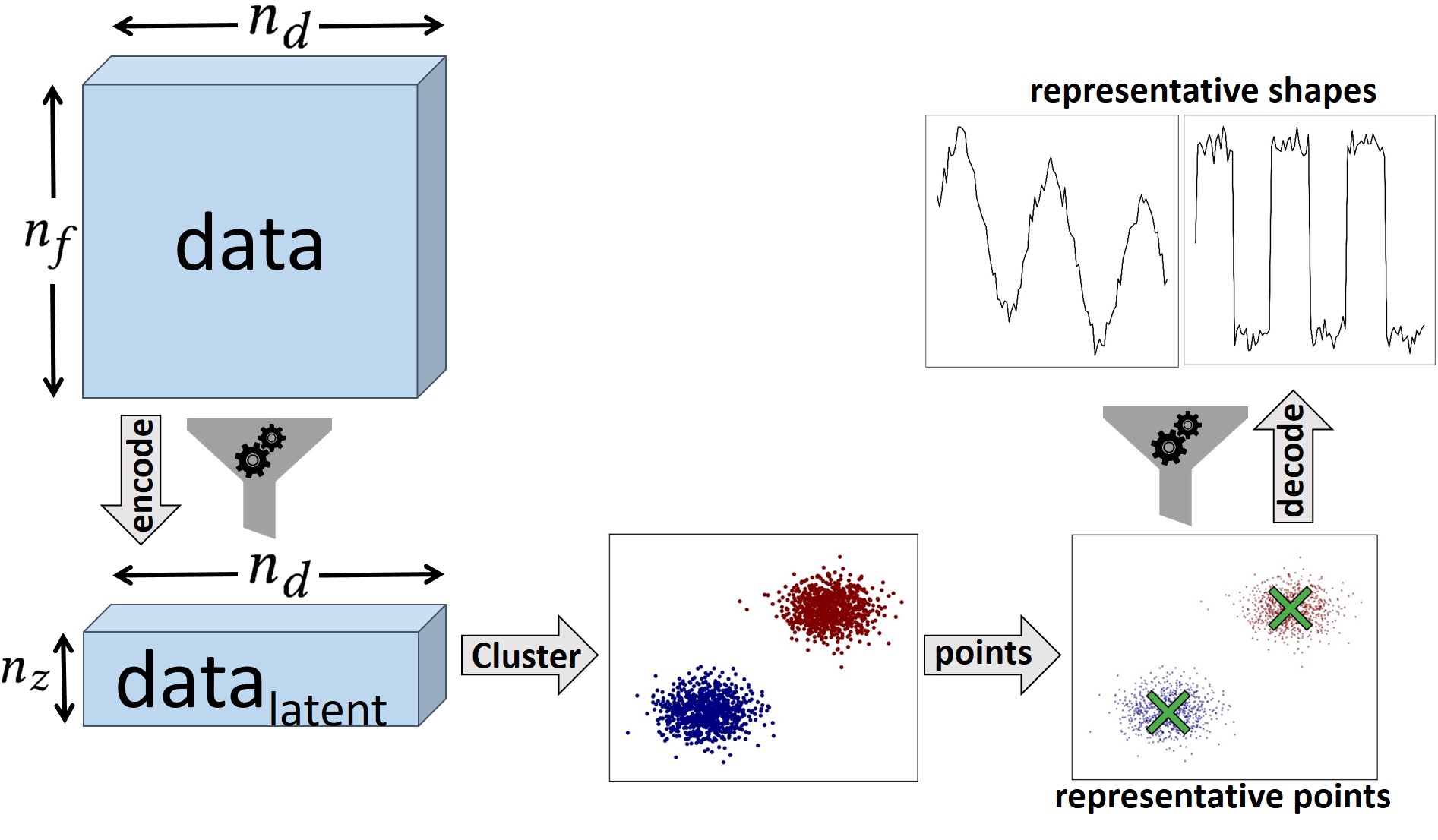
Figure 1: Schematic of the DRAMA framework. First dimensionality reduction (left) is performed on the $n_{d}$ data points down from $n_{f}$ to $n_{z}$ features in the latent space. Unsupervised clustering then splits the data into clusters (here two). The covariance matrix of each label is calculated in the original feature space for the Mahalanobis distance and a prototype is extracted for cluster. This prototype (main component) is then decoded back into the original space (top right) and comparison between the prototypes and test data is performed. Finally anomalies are ranked by their maximum distance to the closest prototype in each case.

II-A Dimensionality reduction

This is the first step of DRAMA procedure. Assume X as a $n_{f}$-dimensional feature vector. Dimensionality reduction translates X into another vector z in an $m$-dimensional space, where $m\ll n$. Good reductions keep as much important information as possible while removing noise and irrelevant information, efficiently encoding the data. In general the reduction will result in loss of information, but is very useful when one wants to work with or visualize the data in lower dimensions or attempts to combat the curse of dimensionality. The inverse process of lifting back up to the original space, i.e. going from z to X will be referred to as decoding hereafter. DRAMA uses both encoding and decoding, with primary component extraction performed in between.

The current version of DRAMA comes with 5 builtin Dimensionality Reduction Techniques (DRT):

• Independent Component Analysis (ICA) [11, 12]

• Non-negative Matrix factorization (NMF) [13]

• Autoencoders (AE) [14]

• Variational AutoEncoders (VAE) [15, 16]

• Principal Component Analysis (PCA) [17, 18]

II-B Prototype extraction

For the second and third steps in DRAMA we now explain prototypes and how they can be extracted. Having encoded the features down to a low-dimensional latent space (here we used 2D) using a choice of DRT, we can efficiently perform unsupervised clustering to detect clusters. Then the primary shapes – the prototypes or archetypes – in the data can be captured by the centers of the detected clusters (see e.g. [19]). We could perform the clustering directly in the high-dimensional feature space before encoding, but this is often computationally unfeasible. Prototype detection can use any of the many existing clustering algorithms. In this study we report results using agglomerative clustering [20] because experiments showed that it was superior to other methods like K-means [21] .

As illustrated in Fig.2, the data is hierarchically split into $2^{n_{s}}$ detected prototypes. We are not concerned with whether the $2^{n_{s}}$ clusters represent true subclasses; $n_{s}$ is simply a hyperparameter designed to find anomalies. Having found the $2^{n_{s}}$ clusters we select the centre of each cluster and can now choose whether or not to decode it to the original, high-dimensional, feature space. Empirically we find that decoding to the original space gives better results. Either way we now have $2^{n_{s}}$ prototypical components representative of the “average” (inlier) data.

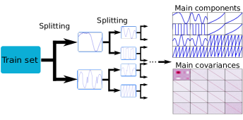
Figure 2: Illustrating prototype extraction process in DRAMA. Splitting can be done iteratively to extract more detailed information about the different shapes in the data, allowing more prototypes to be extracted if the inlier data has a large amount of variation.

II-C Identifying Anomalies

Having decoded (or encoded) the prototypes, the next step is computing the distance between them and each test data point. This requires a metric, $d(x_{i},c_{j})$, where $x_{i}$ are test data points and $c_{j}$ are the prototypes. For any choice of metric the predicted anomalies are then ranked by $\rm{max}_{i}\{\rm{min}_{j}\{d(x_{i},c_{j})\}\}$. The choice of metric is another flexibility of DRAMA. Currently DRAMA includes nine different metrics, given in Table (I).

TABLE I: Metric options available in DRAMA: $d(u,v)$ is the distance between data points $u$ and $v$; $\bar{u}$ is the average of $u$.

Metric	definition
L1	$\sum_{i}{\left|u_{i}-v_{i}\right|}$
L2	${||u-v||}_{2}$
L4	${||u-v||}_{4}$
wL2	${||\frac{u-v}{\sigma}||}_{2}$
wL4	${||\frac{u-v}{\sigma}||}_{4}$
Bray-Curtis	$\sum{|u_{i}-v_{i}|}/\sum{|u_{i}+v_{i}|}$
Chebyshev	$\max_{i}{|u_{i}-v_{i}|}$
Canberra	$\sum_{i}\frac{|u_{i}-v_{i}|}{|u_{i}|+|v_{i}|}$
correlation	$1-\frac{(u-\bar{u})\cdot(v-\bar{v})}{{||(u-\bar{u})||}_{2}{||(v-\bar{v})||}_{2}}$
Mahalanobis	$\sqrt{(u-v)C^{-1}(u-v)^{T}}$

III Datasets for Testing DRAMA

Because of the NFL theorems it is always possible to construct anomaly datasets that make any algorithm look better than any other algorithm. To avoid this we first designed two simulated anomaly detection challenges and then blind-selected several real-world anomaly benchmarks to evaluate DRAMA on, all of which we now describe.

III-A Simulated challenges

There are an infinite number of ways to simulate inliers and anomalies. In this work we consider $10$ different classes of continuous “time series”, shown in Fig.3, representing a wide range of behaviours one might find in the real world.

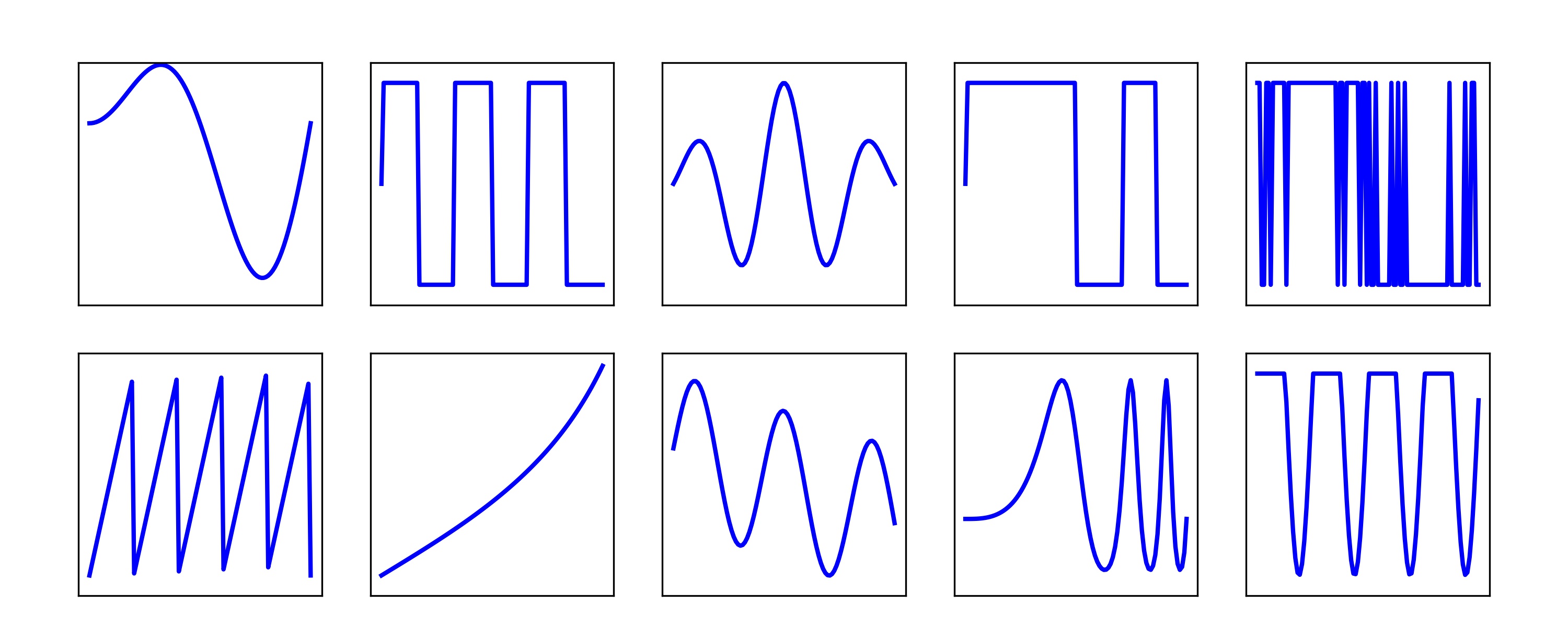
Figure 3: The base classes used for the simulated time-series challenges. Noise and a variety of anomalies were then added on top of these base classes.

These $10$ shapes were perturbed by random Gaussian noise and by random scaling in both the $x$ and $y$ directions. Then we designed two anomaly detection challenges, each with two sub-challenges which differ only in the dimensionality of the data. The challenge details are explained as follows:

• Challenge-I: Compact Anomalies

  In the first challenge compact Gaussian “bump” anomalies were added to the $10$ classes with random location, and amplitude chosen in the range $0.3-0.4$ and width in the range $0.08-0.1$. There were $1000$ inliers and $50$ anomalies for each chosen shape. Finally the noise characteristics were drawn from a mean zero Gaussian with $\sigma=0.3$, comparable to the anomaly amplitude. This task is broken into two sub-challenges, labeled C-Ia and C-Ib, which differ only in the dimensionality of the data. For C-Ia (C-Ib) we chose $n_{f}=100(3000)$ respectively.

• Challenge-II

  The second challenge uses $9$ of the shapes in Fig. (3) to produce 500 inliers with the remaining shape used to produce 50 anomalies. We permute the choice of class used for the anomalies to enhance robustness. Uncorrelated Gaussian noise ($\mu=0$, $\sigma=0.8$) is added in all cases. As before, this challenge is split into two sub-challenges, labeled C-IIa and C-IIb, which again differ only in the dimensionality of the data: $n_{f}=100,3000$ respectively.

III-B Real datasets

In this study we also used $20$ real-world datasets chosen at random from the ODSS database. This is a standard testbed for outlier detection and has been used in many earlier works, including [22, 23, 24]. A summary of the different datasets used, including the dimensionality of the data and number of inliers and outliers, is shown in Table (II).

TABLE II: Real-world dataset summary from the ODSS Benchmark.

Dataset	# points	# dim.	# outliers
lympho	148	18	6
breastw	683	9	239
wine	129	13	10
vertebral	240	6	30
glass	214	9	9
pima	768	8	268
thyroid	3772	6	93
ionosphere	351	33	126
cardio	1831	21	176
wbc	378	30	21
arrhythmia	452	274	66
vowels	1456	12	50
satellite	6435	36	2036
satimage-2	5803	36	71
optdigits	5216	64	150
mammography	11183	6	260
shuttle	49097	9	3511
mnist	7603	100	700
pendigits	6870	16	156
musk	3062	166	97

III-C Scoring metrics

To test for robustness all the algorithms were run 10 times on each test dataset. We then report the means and best performances for two relevant metrics suited for anomaly detection, namely: area under the ROC Curve (AUC) and Rank-Weighted Score (RWS) [25]. Given a ranked list of length $N$ of the most likely outliers, the RWS is defined by:

$$\mbox{RWS}=\frac{1}{N(N+1)}\sum_{i=1}^{N}w_{i}I_{i}$$ (1)

where the weight $w_{i}\equiv N+1-i$ and is large if $i$ is small and decreases to unity for $i=N$. Here $I_{i}$ is an indicator function which is unity if the i-th object is an outlier and $0$ otherwise and the sum is over the top $N$ anomaly candidates. Here we choose $N$ to be the number of anomalies. The RWS rewards algorithms whose anomaly scores correlate well with the true probability of being an anomaly.

IV Results and Discussion

Since DRAMA is, by design, very flexible, it is actually a large number of related algorithms, differing by choice of DRT, clustering, metric etc… As a result, a DRAMA algorithm beat LOF and i-Forest on every simulated data challenge and on 17 out of 20 real-world challenges in terms of AUC. For the problems we study, the cityblock metric and AE & NMF DRTs are the most successful on average. Because of the NFL theorems, DRAMA’s superiority cannot hold in general of course, but the results show that if one DRT or metric does not perform well, another one likely will.

The flexibility of the DRAMA framework is particularly useful when one has seen a few anomalies or outliers. In this case one can learn the best DRT-clustering-metric combination to allow optimal detection of the anomalies. To illustrate this capability we give DRAMA, LOF and i-Forest the ability to learn from a variable number of seen anomalies/outliers. This is used to select optimal hyperparameters for all the algorithms. The results for the two simulated challenges are shown in Fig. 4 and Fig. 5 and for the real datasets in Fig. 6. The figures show both the mean and best results over $10$ runs for each of the challenges and for each algorithm.

While LOF and i-Forest are competitive on the simulated challenges in low dimensions ($n_{f}=100$) DRAMA particularly shines in high dimensions ($n_{f}=3000$). On the real-world datasets we considered which have small numbers of points and dimensions $<300$ the performance of DRAMA and i-Forest are comparable and significantly better than LOF.

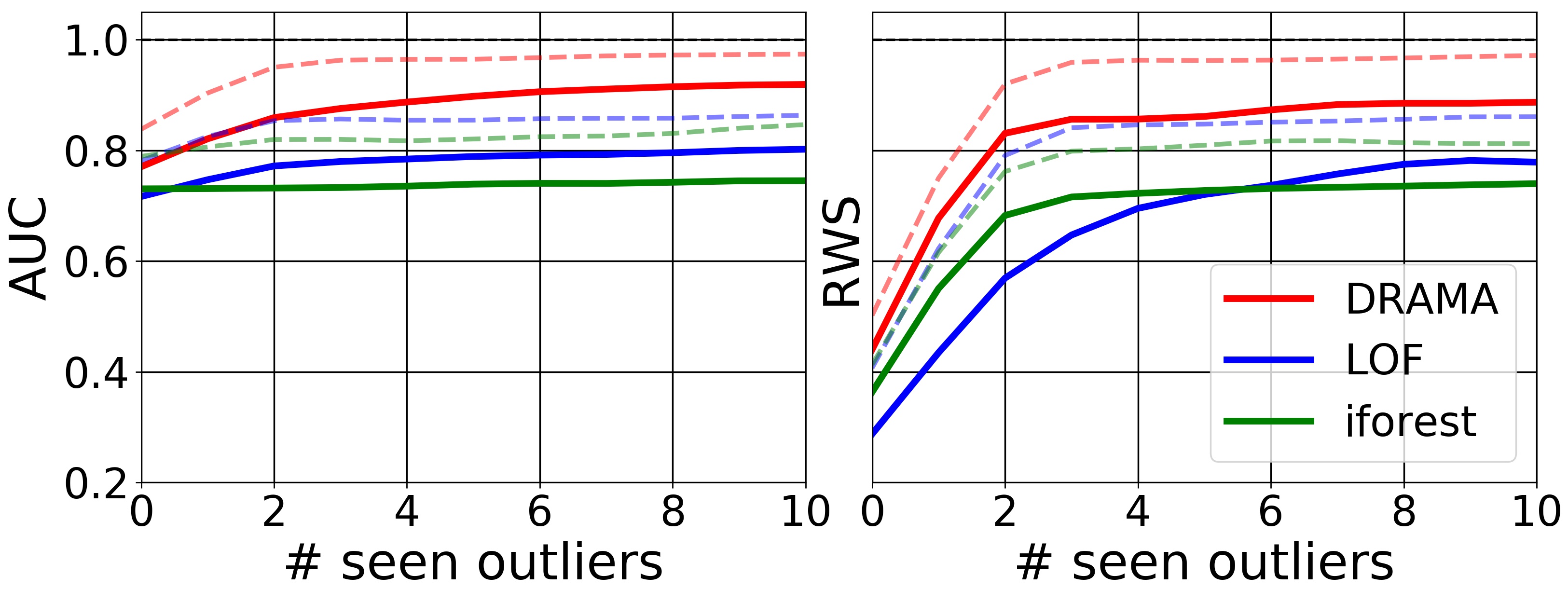
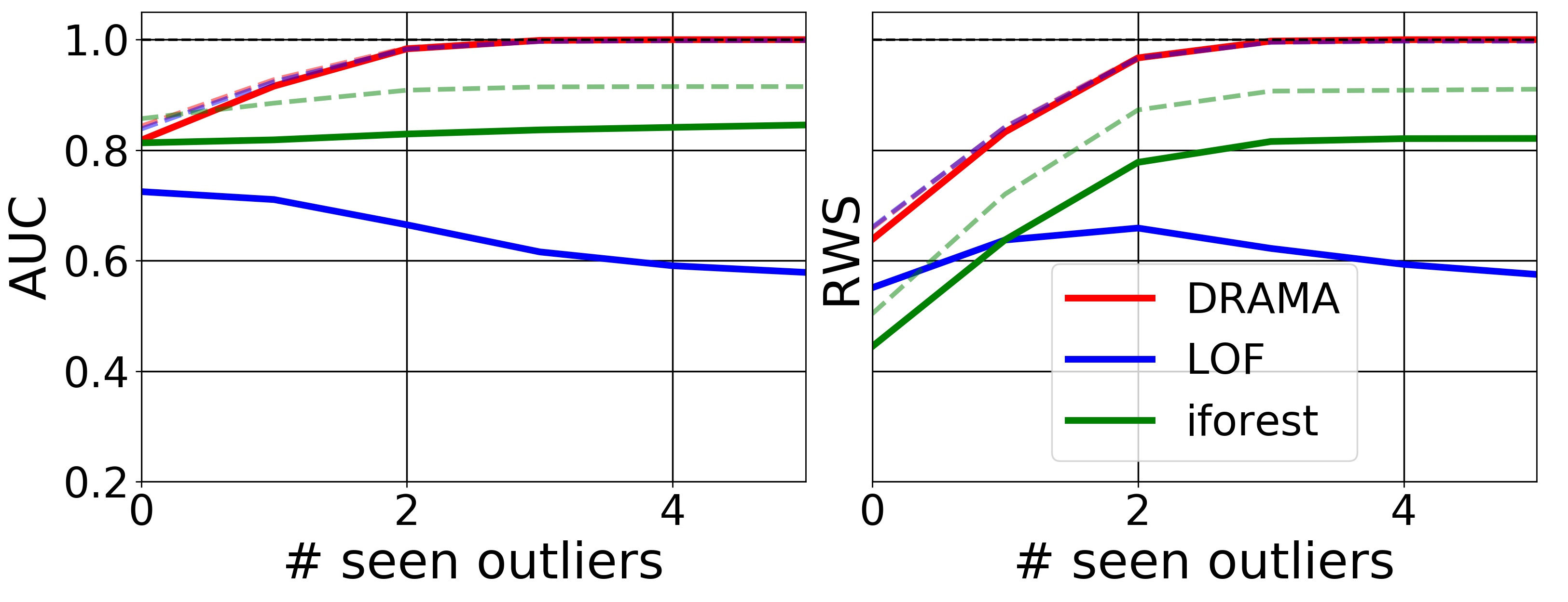
Figure 4: In the compact anomaly challenges, (C-Ia, C-Ib) DRAMA is far superior to both other algorithms for $n_{f}=100$ (top) and $n_{f}=3000$ (bottom), for all numbers of seen anomalies. The solid line is average performance while the dashed line is the maximum performance.

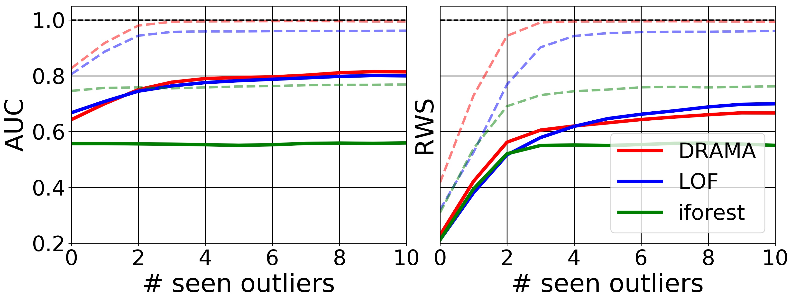
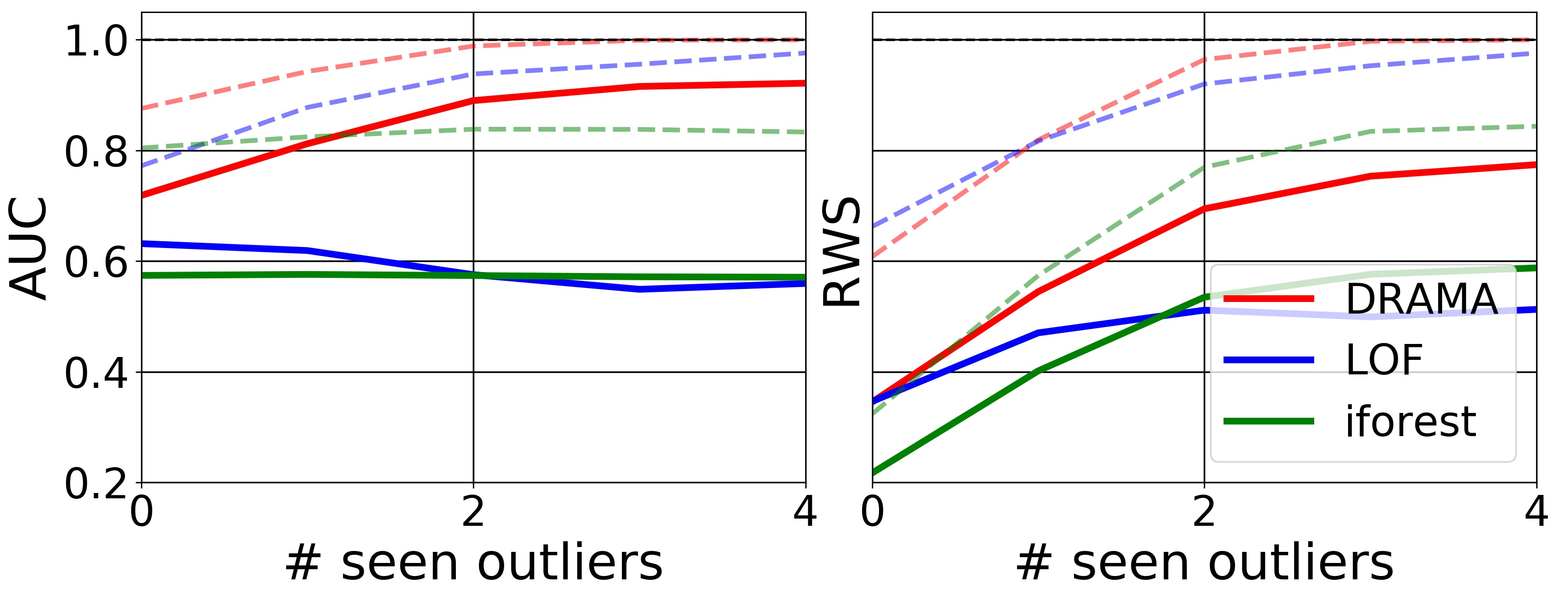
Figure 5: In the 2nd challenge, DRAMA is again equal to or superior to both LOF and iForest for $n_{f}=100$ (top, C-IIa) and $n_{f}=3000$ (bottom, C-IIb). DRAMA particularly shines in the high-dimensional case. The solid line is average performance and the dashed line is the maximum performance, where DRAMA outperforms the other algorithms.

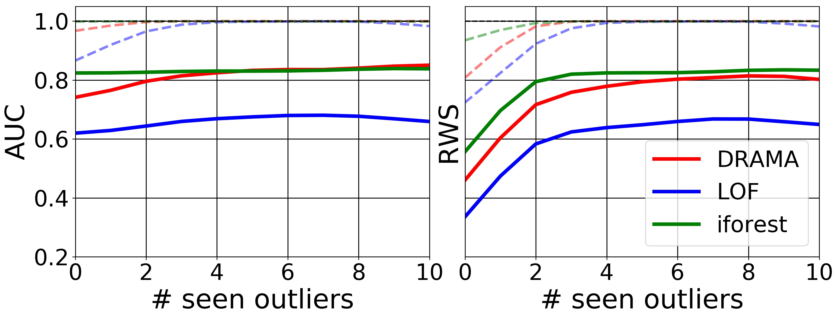
Figure 6: Average (solid lines) and best (dashed lines) performance on the 20 real datasets where iForest and DRAMA outperform LOF. All the datasets have dimensionality less than $300$.

V Conclusions

Anomaly detection is a challenge particularly in the context of and high-dimensional datasets. Here we describe DRAMA, a general python package that uses a range of linear and nonlinear dimensionality reduction transformations, followed by unsupervised clustering to identify prototypes. Potential anomalies are then identified by their distance to the learned prototypes. Currently DRAMA includes five dimensionality reduction algorithms including neural network methods (AE and VAE) along with more standard methods (PCA, ICA, NMF). DRAMA also comes with nine options for the metric.

We evaluated DRAMA performance against the commonly-used algorithms Isolation Forest (i-Forest) and Local Outlier Factor (LOF), averaging different hyperparameter configurations. The large flexibility inherent in DRAMA is particularly attractive in the case of supervised/online anomaly detection where there are known examples of the anomaly of interest because one can optimise for the best DRT-clustering-metric and hyperparameter combination to detect anomalies.

We evaluated DRAMA on a wide variety of simulated and real datasets of up to 3000 dimensions. DRAMA particularly excelled on the simulated time-series data, winning every challenge. On the very inhomogeneous and fairly low-dimensional real-world datasets we tested, DRAMA was highly competitive with LOF and i-Forest, showing that dimensionality reduction and clustering is a valuable approach to anomaly detection.

Finally we note that it would be interesting to optimize DRAMA for novelty detection and anomaly detection in images.

References

- [1] G. Williams and Z. Huang, “Mining the knowledge mine,” Advanced Topics in Artificial Intelligence, pp. 340–348, 1997.
- [2] W. DuMouchel and M. Schonlau, “A fast computer intrusion detection algorithm based on hypothesis testing of command transition probabilities.” in KDD, 1998, pp. 189–193.
- [3] T. Pham and S. Lee, “Anomaly detection in the bitcoin system-a network perspective,” arXiv preprint arXiv:1611.03942, 2016.
- [4] C. C. Aggarwal, A. Hinneburg, and D. A. Keim, “On the surprising behavior of distance metrics in high dimensional spaces,” in ICDT, vol. 1. Springer, 2001, pp. 420–434.
- [5] K. Beyer, J. Goldstein, R. Ramakrishnan, and U. Shaft, “When is “nearest neighbor” meaningful?” in International conference on database theory. Springer, 1999, pp. 217–235.
- [6] H. W. Lin, M. Tegmark, and D. Rolnick, “Why does deep and cheap learning work so well?” Journal of Statistical Physics, vol. 168, no. 6, pp. 1223–1247, 2017.
- [7] F. Pedregosa, G. Varoquaux, A. Gramfort, V. Michel, B. Thirion, O. Grisel, M. Blondel, P. Prettenhofer, R. Weiss, V. Dubourg, J. Vanderplas, A. Passos, D. Cournapeau, M. Brucher, M. Perrot, and E. Duchesnay, “Scikit-learn: Machine learning in Python,” Journal of Machine Learning Research, vol. 12, pp. 2825–2830, 2011.
- [8] J. Allaire, D. Eddelbuettel, N. Golding, and Y. Tang, tensorflow: R Interface to TensorFlow, 2016. [Online]. Available: https://github.com/rstudio/tensorflow
- [9] M. M. Breunig, H.-P. Kriegel, R. T. Ng, and J. Sander, “Lof: identifying density-based local outliers,” in ACM sigmod record, vol. 29, no. 2. ACM, 2000, pp. 93–104.
- [10] F. T. Liu, K. M. Ting, and Z.-H. Zhou, “Isolation forest,” in Data Mining, 2008. ICDM’08. Eighth IEEE International Conference on. IEEE, 2008, pp. 413–422.
- [11] A. Hyvärinen, J. Karhunen, and E. Oja, Independent component analysis. John Wiley & Sons, 2004, vol. 46.
- [12] G. R. Naik, “Introduction: Independent component analysis,” in Independent Component Analysis for Audio and Biosignal Applications. InTech, 2012.
- [13] M. W. Berry, M. Browne, A. N. Langville, V. P. Pauca, and R. J. Plemmons, “Algorithms and applications for approximate nonnegative matrix factorization,” Computational statistics & data analysis, vol. 52, no. 1, pp. 155–173, 2007.
- [14] G. E. Hinton and R. S. Zemel, “Autoencoders, minimum description length and helmholtz free energy,” in Advances in neural information processing systems, 1994, pp. 3–10.
- [15] D. P. Kingma and M. Welling, “Auto-encoding variational bayes,” arXiv preprint arXiv:1312.6114, 2013.
- [16] D. J. Rezende, S. Mohamed, and D. Wierstra, “Stochastic backpropagation and approximate inference in deep generative models,” arXiv preprint arXiv:1401.4082, 2014.
- [17] K. Pearson, “Liii. on lines and planes of closest fit to systems of points in space,” The London, Edinburgh, and Dublin Philosophical Magazine and Journal of Science, vol. 2, no. 11, pp. 559–572, 1901.
- [18] H. Hotelling, “Analysis of a complex of statistical variables into principal components.” Journal of educational psychology, vol. 24, no. 6, p. 417, 1933.
- [19] M. Biehl, B. Hammer, and T. Villmann, “Prototype-based models in machine learning,” Wiley Interdisciplinary Reviews: Cognitive Science, vol. 7, no. 2, pp. 92–111, 2016.
- [20] W. H. Day and H. Edelsbrunner, “Efficient algorithms for agglomerative hierarchical clustering methods,” Journal of classification, vol. 1, no. 1, pp. 7–24, 1984.
- [21] J. A. Hartigan and M. A. Wong, “Algorithm as 136: A k-means clustering algorithm,” Journal of the Royal Statistical Society. Series C (Applied Statistics), vol. 28, no. 1, pp. 100–108, 1979.
- [22] C. C. Aggarwal and S. Sathe, “Theoretical foundations and algorithms for outlier ensembles,” ACM SIGKDD Explorations Newsletter, vol. 17, no. 1, pp. 24–47, 2015.
- [23] S. Sathe and C. Aggarwal, “Lodes: Local density meets spectral outlier detection,” in Proceedings of the 2016 SIAM International Conference on Data Mining. SIAM, 2016, pp. 171–179.
- [24] S. Rayana and L. Akoglu, “Less is more: Building selective anomaly ensembles,” ACM Transactions on Knowledge Discovery from Data (TKDD), vol. 10, no. 4, p. 42, 2016.
- [25] E. Roberts, B. A. Bassett, and M. Lochner, “Bayesian anomaly detection and classification,” arXiv preprint arXiv:1902.08627, 2019.