Clustering of primordial black holes formed in a matter-dominated epoch

Abstract

In the presence of the local-type primordial non-Gaussianity, it is known that the clustering of primordial black holes (PBHs) emerges even on superhorizon scales at the formation time. This effect has been investigated in the high-peak limit of the PBH formation in the radiation-dominated epoch in the literature. There is another possibility that the PBH formation takes place in the early matter-dominated epoch. In this scenario, the high-peak limit is not applicable because even initially small perturbations grow and can become a PBH. We first derive a general formula to estimate the clustering of PBHs with primordial non-Gaussianity without assuming the high-peak limit, and then apply this formula to a model of PBH formation in a matter-dominated epoch. Clustering is less significant in the case of the PBH formation in the matter-dominated epoch than that in the radiation-dominated epoch. Nevertheless, it is much larger than the Poisson shot noise in many cases. Relations to the constraints of the isocurvature perturbations by the cosmic microwave background radiation are quantitatively discussed.

I Introduction

Primordial black holes (PBHs) have recently attracted much attention Carr:2009jm . This is mainly because of the following reasons. First, we can fit the signals of gravitational waves Bird:2016dcv ; Clesse:2016vqa ; Sasaki:2016jop ; Sasaki:2018dmp , which have been reported by LIGO and/or Virgo. For example, in Ref. Abbott:2016blz , the gravitational wave emitted from the merger events of the binaries are fitted by assuming homogeneously distributed PBHs with masses of $M_{\rm PBH}\sim{\cal O}(10)M_{\odot}$. Second, PBHs with $M_{\rm PBH}\sim{\cal O}(10^{-17})M_{\odot}$ Carr:2009jm – ${\cal O}(10^{-11})M_{\odot}$ Niikura:2017zjd can explain all the cold dark matter (CDM) components in the Universe (see, e.g., Refs. Carr:2016drx ; Juan1996PhRvD ; Clesse2015PBH ). Third, we can fit the Optical Gravitational Lensing Experiment (OGLE) ultrashort-timescale microlensing events Niikura:2019kqi by PBHs with their masses of $M_{\rm PBH}\sim{\cal O}(10^{-5})M_{\odot}$. Fourth, PBHs with $M_{\rm PBH}\sim{\cal O}(10^{3.5})$ – ${\cal O}(10^{5})M_{\odot}$ may become seeds for formations of supermassive black holes (SMBHs) by assuming a subsequent sub-Eddington accretion rate on to the seed Kawasaki:2012kn ; Kohri2014SMBH ; Kawasaki:2019iis .

Concerning a possible mechanism to produce PBHs, we expect that high peaks of curvature perturbation (or density perturbation $\delta\gtrsim\delta_{\rm c}\simeq 0.3$–$0.4$ Carr:1975qj ; Harada:2013epa ) at small scales collapsed into PBHs in the radiation-dominated (RD) Universe. It is known that such a high value of curvature perturbation at small scales is produced by various models of inflation Inomata:2017vxo ; Lyth:2011kj ; Kohri:2007qn ; Pi17 ; Gao:2018pvq , preheating after inflation Frampton:2010sw ; Martin:2019nuw , the curvaton in the inflationary Universe Kawasaki:2012wr ; Kohri:2012yw ; Bugaev:2012ai , Q-ball formations Cotner:2019ykd ; Kawasaki:2019iis and so forth.

Recently, the effects of non-Gaussianities have been discussed in investigating more precise properties of the PBH formation. For instance, Refs. Kawasaki:2019mbl ; DeLuca:2019qsy ; Young:2019yug focused on a nonlinear relation between the density fluctuations and the primordial curvature perturbations on superhorizon scales, and Ref. Yoo:2018esr developed a formula for the PBH abundance with taking this nonlinearity into account in the peak theory.

As another type of non-Gaussianities, the primordial non-Gaussianity of the curvature perturbations, which would be a probe of the inflationary mechanism, has been also considered. It was found that the primordial non-Gaussianity has a significant impact on the PBH abundance (see, e.g., Refs. Atal:2019cdz ; Yoo:2019pma and references therein). Furthermore, some types of the primordial non-Gaussianity could affect not only the PBH abundance but also the spatial clustering of PBHs. There have been lots of works about this issue. In common understanding, if the primordial curvature perturbations obey Gaussian statistics, the distribution of the formed PBHs would be spatially uniform; that is, the distribution is Poissonian (see, e.g., Refs. Chi06 ; Ali18 ; Desjacques:2018wuu ; SY19 and references therein). On the other hand, if the probability distribution function of the primordial curvature perturbations would have the non-Gaussianity which can induce the coupling between the long and short wavelength modes, the formed PBHs would spatially clustered even on super-Hubble scales TY15 ; Young:2015kda ; SY19 . Such clustering of PBHs can be observed as the matter isocurvature fluctuations in the cosmic microwave background (CMB) and the large-scale structure, if the PBHs are a part of the CDM component TY15 ; Young:2015kda . As another observational impact of the PBH clustering, the effect on the merger rate of the PBH binary system, which should be an important parameter for the LIGO/Virgo gravitational wave event, recently has been investigated Raidal:2017mfl ; Ballesteros:2018swv ; Bringmann:2018mxj ; Ding:2019tjk ; Vaskonen:2019jpv .

The PBH formations are frequently assumed to take place in the RD epoch. However, in the early Universe, oscillating energies of nonrelativistic massive scalar fields such as the inflaton field or curvaton field of which the energy density scales as $\rho\propto a^{-3}$ with scale factor $a=a(t)$ may dominate the energy density of the Universe until their decays (i.e., until the reheating time). In this case, an early matter-dominated (MD) epoch could be realized before the RD epoch.

More concretely, moduli or dilaton fields, which are predicted in particle physics models beyond the standard model such as supergravity and/or superstring theory, tend to have a long lifetime. That is because they decay only through gravitational interaction. For example, with their masses of the order of weak scale, the lifetime can be ${\cal O}(1)~{}{\rm sec}$ and reheating temperature after its domination becomes $T_{\mathrm{R}}\sim O(1)$ MeV. Hasegawa:2019jsa (see also Refs. Kawasaki:1999na ; Kawasaki:2000en ; Hannestad:2004px ; Ichikawa:2005vw ; deSalas:2015glj ). In this case, PBHs with their masses up to $M_{\rm PBH}\lesssim{\cal O}(10^{3})\,M_{\odot}$ could be produced in the early MD epoch.

In this paper, we investigate the clustering property of the PBHs formed in the early MD epoch in the presence of local-type non-Gaussianity. In Refs. TY15 ; Young:2015kda ; SY19 , which focus on the PBH formation in the RD epoch, a simple high-peak formalism is employed to evaluate the two-point correlation function or the power spectrum of the spatial fluctuations of PBH number density, which characterize the PBH clustering. This is because in the RD epoch PBHs are considered to be simply formed through the spherical gravitational collapse of the overdense region with Hubble scales. On the other hand, the formation of PBHs in the early MD epoch are completely different from the ones in the RD epoch. Because perturbations evolve nonspherically in MD epochs under negligible pressure, even if $\delta\ll\delta_{\rm c}$, a PBH can form once a region is enclosed by its event horizon Khlopov:1980mg ; Polnarev:1982 ; Har16 . By considering finite angular momentum in each patch of horizon, the number density of the PBHs produced in the early MD epoch is suppressed exponentially due to their own spins Har17 (see also Ref. Kokubu:2018fxy for an additional suppression of the number density due to inhomogeneities). Therefore, it is a nontrivial question which dominates between the clustering of PBHs and the Poisson noise of the PBHs formed in the MD epoch.

We employ a model of Refs. Har16 ; Har17 for the PBH formation in the MD epoch, taking into account the nonlinear, nonspherical evolutions of the matter density with the Zel’dovich approximation Zel70 and the PBH formation with the hoop conjecture Tho72 . In order to carefully treat the details of the formation process, we make use of a method of the integrated perturbation theory (iPT) Mat95 ; Mat11 ; Mat12 ; YM13 ; Mat14 . The iPT is a general framework to predict the clustering properties of biased fields and is able to take into account the effects of nonlinear evolutions of clustering, redshift-space distortions, primordial non-Gaussianity, etc. In this paper, we are interested in the clustering of PBHs at the formation time, and the iPT is used only in estimating a contribution of primordial non-Gaussianity to the initial clustering of PBHs.

The paper is organized as follows. In Sec. II, a general consequence of the iPT for the initial power spectrum of PBHs due to the primordial local-type non-Gaussianity is summarized. It is shown that the iPT can successfully reproduce the previous results in the high-peak limit. In Sec. III, the formula for the PBH clustering in the MD epoch, which is a main result of this paper, is derived. Observational implications are discussed in Sec. IV. Our conclusions are given in Sec. V. Technical details of the derivation of our formulas are given in Appendixes A and B. Detailed discussion on the observational constraints is given in Appendix C.

II Initial power spectrum of PBHs with primordial non-Gaussianity

The PBHs are considered to be biased objects of the energy density in the early Universe. In this section, we generally consider the biased power spectrum in the presence of local-type non-Gaussianity, by making use of the iPT formalism. The results of this section is valid in both the RD and MD epochs.

II.1 Local-type non-Gaussianity

We consider the primordial non-Gaussianity characterized by higher-order polyspectra of the curvature perturbations on the comoving slice $\mathcal{R}$ as

$$\left\langle\mathcal{R}(\bm{k}_{1})\mathcal{R}(\bm{k}_{2})\right\rangle_{\mathrm{c}}=(2\pi)^{3}\delta_{\mathrm{D}}^{3}(\bm{k}_{1}+\bm{k}_{2})P_{\mathcal{R}}(k_{1}),$$ (1)

$$\left\langle\mathcal{R}(\bm{k}_{1})\mathcal{R}(\bm{k}_{2})\mathcal{R}(\bm{k}_{3})\right\rangle_{\mathrm{c}}=(2\pi)^{3}\delta_{\mathrm{D}}^{3}(\bm{k}_{1}+\bm{k}_{2}+\bm{k}_{3})B_{\mathcal{R}}(\bm{k}_{1},\bm{k}_{2},\bm{k}_{3}),$$ (2)

$$\left\langle\mathcal{R}(\bm{k}_{1})\mathcal{R}(\bm{k}_{2})\mathcal{R}(\bm{k}_{3})\mathcal{R}(\bm{k}_{4})\right\rangle_{\mathrm{c}}=(2\pi)^{3}\delta_{\mathrm{D}}^{3}(\bm{k}_{1}+\bm{k}_{2}+\bm{k}_{3}+\bm{k}_{4})$$

$$\hskip 132.0pt\times T_{\mathcal{R}}(\bm{k}_{1},\bm{k}_{2},\bm{k}_{3},\bm{k}_{4}),$$ (3)

where $\langle\cdots\rangle_{\mathrm{c}}$ denotes the cumulant, or the connected part of correlations, and $P_{\mathcal{R}}$, $B_{\mathcal{R}}$, and $T_{\mathcal{R}}$ are called the power spectrum, bispectrum, and trispectrum, respectively. For the local-type non-Gaussianity, the higher-order polyspectra are given by BSW06

$$B_{\mathcal{R}}(\bm{k}_{1},\bm{k}_{2},\bm{k}_{3})=\frac{6}{5}f_{\mathrm{NL}}\left[P_{\mathcal{R}}(k_{1})P_{\mathcal{R}}(k_{2})+\mathrm{cyc.}\right],$$ (4)

$$T_{\mathcal{R}}(\bm{k}_{1},\bm{k}_{2},\bm{k}_{3},\bm{k}_{4})=\frac{54}{25}g_{\mathrm{NL}}\left[P_{\mathcal{R}}(k_{1})P_{\mathcal{R}}(k_{2})P_{\mathcal{R}}(k_{3})+\mathrm{3\ perms}\right]$$

$$\hskip 54.0pt+\tau_{\mathrm{NL}}\left[P_{\mathcal{R}}(k_{1})P_{\mathcal{R}}(k_{2})P_{\mathcal{R}}(k_{13})+\mathrm{11\ perms}\right],$$ (5)

where $k_{13}\equiv|\bm{k}_{1}+\bm{k}_{3}|$ etc., and $f_{\mathrm{NL}}$, $g_{\mathrm{NL}}$, and $\tau_{\mathrm{NL}}$ are the parameters of local-type non-Gaussianity, and perms stands for permutations and cyc stands for cyclic permutations. If the primordial curvature perturbations emerge from the quantum fluctuations of a single scalar field, there is a relation, $\tau_{\mathrm{NL}}=(36/25){f_{\mathrm{NL}}}^{2}$ Boubekeur:2005fj . If multiple scalar fields contribute, there is an inequality, $\tau_{\mathrm{NL}}>(36/25){f_{\mathrm{NL}}}^{2}$ SY08 .

The relation at linear order between comoving curvature perturbations $\mathcal{R}$ and the linear density contrast $\delta_{\mathrm{L}}$ on comoving slices is given by LL00 ; YBS14

$$\delta_{\mathrm{L}}(\bm{k})=\mathcal{M}(k)\mathcal{R}(\bm{k}),$$ (6)

where the proportional factor in the RD and MD epochs is given by

$$\mathcal{M}(k)\equiv\frac{2+2w}{5+3w}\frac{k^{2}T(k)}{a^{2}H^{2}},$$ (7)

where $w=p/\rho$ is the parameter of the equation of state and $H=\dot{a}/a$ is the Hubble parameter. The transfer function $T(k)$ describes the evolution on subhorizon scales, and the time dependencies in various functions are suppressed in our notations for simplicity. For example, $T(k,\eta)=[\sin(k\eta)-k\eta\cos(k\eta)]/[3(k\eta)^{3}]$ in the RD epoch, where $\eta$ is the conformal time. In the applications to PBHs in the following sections, we are interested in the superhorizon scales at the formation epoch of PBHs, where we can safely put $T(k)=1$.

II.2 Power spectrum in the presence of local-type non-Gaussianity

In the iPT formalism, the renormalized bias functions in Lagrangian space are defined by Mat11 ; Mat12

$$c^{\mathrm{L}}_{n}(\bm{k}_{1},\ldots,\bm{k}_{n})=(2\pi)^{3n}\int\frac{d^{3}k}{(2\pi)^{3}}\left\langle\frac{\delta^{n}\delta^{\mathrm{L}}_{X}(\bm{k})}{\delta\delta_{\mathrm{L}}(\bm{k}_{1})\cdots\delta\delta_{\mathrm{L}}(\bm{k}_{n})}\right\rangle,$$ (8)

where $\delta^{\mathrm{L}}_{X}(\bm{k})$ is the density contrast of the biased objects in Lagrangian space as a functional of the linear density contrast, and $\delta/\delta\delta_{\mathrm{L}}(\bm{k})$ is a functional derivative.

The iPT formalism applies to any biased objects in general, while in this paper we identify the biased objects as PBHs in later sections. In Ref. YM13 , the power spectrum of biased objects in the large-scale limit, where nonlinear evolution of the matter density field is negligible, is calculated by the formalism of iPT in the late-time MD epoch. Substituting $\mathcal{M}(k)$ of this literature by $(5/3)\mathcal{M}(k)$ in this paper, the same expressions as Eqs. (23) and (34) of Ref. YM13 hold in both the RD and MD epochs. Thus the result of iPT for the power spectrum of the biased objects in the large-scale limit is given by

$$P_{X}(k)\simeq [b_{1}(k)]^{2}P_{\mathrm{L}}(k)$$

$$+\frac{12}{5}f_{\mathrm{NL}}b_{1}(k)\frac{P_{\mathrm{L}}(k)}{\mathcal{M}(k)}\int\frac{d^{3}p}{(2\pi)^{3}}c^{\mathrm{L}}_{2}(\bm{p},-\bm{p})P_{\mathrm{L}}(p)$$ (9)

$$+\left(\frac{54}{25}g_{\mathrm{NL}}+2\tau_{\mathrm{NL}}\right)b_{1}(k)\frac{P_{\mathrm{L}}(k)}{\mathcal{M}(k)}\int\frac{d^{3}p_{1}}{(2\pi)^{3}}\frac{d^{3}p_{2}}{(2\pi)^{3}}$$

$$\quad\times c^{\mathrm{L}}_{3}(\bm{p}_{1},\bm{p}_{2},-\bm{p}_{1}-\bm{p}_{2})\frac{\mathcal{M}(p_{12})}{\mathcal{M}(p_{1})\mathcal{M}(p_{2})}P_{\mathrm{L}}(p_{1})P_{\mathrm{L}}(p_{2})$$

$$+\tau_{\mathrm{NL}}\frac{P_{\mathrm{L}}(k)}{\mathcal{M}^{2}(k)}\left[\int\frac{d^{3}p}{(2\pi)^{3}}c^{\mathrm{L}}_{2}(\bm{p},-\bm{p})P_{\mathrm{L}}(p)\right]^{2}$$

$$+P_{\mathrm{const}},$$ (10)

where $P_{\mathrm{L}}(k)$ is the power spectrum of the linear density field $\delta_{\mathrm{L}}$, $b_{1}(k)\equiv 1+c^{\mathrm{L}}_{1}(k)$ is the linear bias parameter in Eulerian space, and $P_{\mathrm{const}}$ is the higher-order correction terms which are constant in the large-scale limit of $k\rightarrow 0$.

The most dominant contribution in the large-scale limit of $k\rightarrow 0$ is given by the term with a factor $\mathcal{M}^{-2}(k)$, because $\mathcal{M}(k)\sim k^{2}$. The corresponding term of the most dominant contribution is the last term but one in Eq. (10). The factor $\mathcal{M}(k)$ is sufficiently small for $k\ll aH=R^{-1}$, where $R$ is the comoving horizon scale which gives the mass scale $M\sim 4\pi R^{3}/3$ of PBHs in later sections. Therefore, the most dominant term of the power spectrum in the large-scale limit $k\ll R^{-1}$ is given by

$$P_{X}(k)\simeq\tau_{\mathrm{NL}}{C_{2}}^{2}\frac{P_{\mathrm{L}}(k)}{\mathcal{M}^{2}(k)}=\tau_{\mathrm{NL}}{C_{2}}^{2}P_{\mathcal{R}}(k),$$ (11)

where

$$C_{2}\equiv\int\frac{d^{3}p}{(2\pi)^{3}}c^{\mathrm{L}}_{2}(\bm{p},-\bm{p})P_{\mathrm{L}}(p).$$ (12)

Equation (11) is the general prediction of iPT for the biased power spectrum with local-type non-Gaussianity in the large-scale limit of $k\rightarrow 0$. There appears a strongly scale-dependent bias, $P_{X}(k)/P_{\mathrm{L}}(k)\propto\mathcal{M}^{-2}(k)\propto k^{-4}$ in the large-scale limit. The same scaling property is also derived from the peak-background split in the halo model SL11 ; BFGS13 . The amplitude of the scale-dependent bias is proportional to the product $\tau_{\mathrm{NL}}{C_{2}}^{2}$, and the factor $C_{2}$ depends on the formation process of the biased objects.

II.3 High-peak limit of thresholded regions

The result of Eq. (11) in the previous subsection is quite general for any biased objects. To determine the amplitude, the factor $C_{2}$ should be estimated. This factor has a simple form in a high-peak limit, which we first consider here. The high-peak limit of thresholded regions is frequently considered as an approximation of formation sites of PBHs in the RD epoch Chi06 . The number density of the collapsed objects above a threshold $\delta_{\mathrm{c}}$ is given by

$$n_{\mathrm{th}}(\bm{x})=\frac{\bar{n}_{\mathrm{th}}}{\beta^{\mathrm{th}}_{0}}\Theta\left[\delta_{R}(\bm{x})-\delta_{\mathrm{c}}\right],$$ (13)

where $\Theta(x)$ is the Heaviside step function,

$$\delta_{R}(\bm{x})=\int\frac{d^{3}k}{(2\pi)^{3}}e^{i\bm{k}\cdot\bm{x}}\delta_{\mathrm{L}}(\bm{k})W(kR)$$ (14)

is the smoothed density contrast with a smoothing radius $R$, $W(kR)$ is the window function, $\bar{n}_{\mathrm{th}}=\langle n_{\mathrm{th}}(\bm{x})\rangle$ is the mean number density, and

$$\beta^{\mathrm{th}}_{0}\equiv\left\langle\Theta\left(\delta_{R}-\delta_{\mathrm{c}}\right)\right\rangle$$ (15)

is the production probability. The number density of Eq. (13) is an example of the local Lagrangian bias, and the renormalized bias in this case is given by (Eq. (89) of Ref. Mat11 )

$$c^{\mathrm{L}}_{n}(\bm{k}_{1},\ldots,\bm{k}_{n})=\frac{1}{\bar{n}_{\mathrm{th}}}\left\langle\frac{d^{n}n_{\mathrm{th}}}{d{\delta_{R}}^{n}}\right\rangle W(k_{1}R)\cdots W(k_{n}R).$$ (16)

Specifically, we have

$$c^{\mathrm{L}}_{n}(\bm{k}_{1},\ldots,\bm{k}_{n})=\frac{\beta^{\mathrm{th}}_{n}}{\beta^{\mathrm{th}}_{0}}W(k_{1}R)\cdots W(k_{n}R),$$ (17)

where

$$\beta^{\mathrm{th}}_{n}\equiv\left\langle\delta_{\mathrm{D}}^{(n-1)}\left(\delta_{R}-\delta_{\mathrm{c}}\right)\right\rangle,$$ (18)

and $\delta_{\mathrm{D}}^{(n-1)}(x)=d^{n-1}\delta_{\mathrm{D}}(x)/dx^{n-1}=d^{n}\Theta(x)/dx^{n}$ is the $(n-1)$th derivative of the Dirac delta function, $\delta_{\mathrm{D}}(x)=d\Theta(x)/dx$.

Up to the lowest order in non-Gaussianity parameters, the averages of Eqs. (15) and (18) can be estimated with Gaussian statistics, provided that they are substituted in Eqs. (11) and (12). Using the variance of the smoothed density contrast,

$$\sigma^{2}\equiv\int\frac{k^{2}dk}{2\pi^{2}}P_{\mathrm{L}}(k)W^{2}(kR),$$ (19)

we have

$$\beta^{\mathrm{th}}_{n} =\frac{1}{\sqrt{2\pi}\sigma}\int_{-\infty}^{\infty}d\delta\,e^{-\delta^{2}/(2\sigma^{2})}\delta_{\mathrm{D}}^{(n-1)}\left(\delta-\delta_{\mathrm{c}}\right)$$

$$=\frac{1}{\sqrt{2\pi}\sigma^{n}}H_{n-1}(\nu)e^{-\nu^{2}/2},$$ (20)

where $\nu\equiv\delta_{\mathrm{c}}/\sigma$, and $H_{m}(x)=e^{x^{2}/2}(-d/dx)^{n}e^{-x^{2}/2}$ is the Hermite polynomial. If we define

$$H_{-1}(x)\equiv\sqrt{\frac{\pi}{2}}e^{x^{2}/2}\mathrm{erfc}\left(\frac{x}{\sqrt{2}}\right),$$ (21)

Eq. (20) holds also in the case of $n=0$ Mat95 . Substituting Eq. (17) with $n=2$ into Eq. (12), we have

$$C_{2}=\frac{H_{1}(\nu)}{H_{-1}(\nu)},$$ (22)

and Eq. (11) reduces to

$$P_{\mathrm{PBH}}(k) =\left(\frac{H_{1}(\nu)}{H_{-1}(\nu)}\right)^{2}\tau_{\mathrm{NL}}\frac{P_{\mathrm{L}}(k)}{\mathcal{M}^{2}(k)}$$

$$=\frac{2\nu^{2}}{\pi e^{\nu^{2}}}\left[\mathrm{erfc}\left(\frac{\nu}{\sqrt{2}}\right)\right]^{-2}\tau_{\mathrm{NL}}\frac{P_{\mathrm{L}}(k)}{\mathcal{M}^{2}(k)},$$ (23)

when the biased objects are identified as PBHs.

The PBH formation in the RD epoch is frequently modeled by a high-peak limit $\nu\rightarrow\infty$ of the thresholded regions. In the high-peak limit, we have $H_{m}(\nu)\rightarrow\nu^{m}$, including $m=-1$. In this limit, we have $C_{2}\simeq\nu^{2}$, and Eq. (23) reduces to a simple expression,

$$P_{\mathrm{PBH}}(k)\simeq\nu^{4}\tau_{\mathrm{NL}}\frac{P_{\mathrm{L}}(k)}{\mathcal{M}^{2}(k)}=\nu^{4}\tau_{\mathrm{NL}}P_{\mathcal{R}}(k).$$ (24)

This equation is consistent with the results of Refs. TY15 ; SY19 .

III Initial clustering of PBHs formed in a matter-dominated epoch in the presence of primordial non-Gaussianity

In the previous section, we found that the dominant contribution in the large-scale limit to the initial power spectrum is given by Eq. (11) in the presence of local-type non-Gaussianity. In that expression, the integral $C_{2}$ of Eq. (12), together with non-Gaussianity parameter $\tau_{\mathrm{NL}}$, determines the amplitude of the initial power spectrum of PBHs. As noted in the last section, this integral in the high-peak limit is given by $C_{2}\simeq\nu^{2}$, when the PBH is assumed to form with a condition, $\delta\geq\nu\sigma$. The high-peak limit is satisfied in a usual assumption that the PBH formed in the RD epoch where $\nu\sim\mathcal{O}(10)$ Chi06 ; TY15 ; Ali18 . However, there is a possibility that the high-peak limit is not satisfied in the PBH formation. For example, there are scenarios in which the PBHs are formed in a MD epoch Har16 ; Har17 , in which case the high-peak limit is not appropriate. In the PBH formation in a MD epoch, nonspherical effects in gravitational collapse play a crucial role.

In this section, we apply a model of Refs. Har16 ; Har17 . In the model, the Zel’dovich approximation Zel70 , Thorne’s hoop conjecture Tho72 , and Doroshkevich’s probability distribution Dor70 are combined to predict the PBH formation in a MD epoch.

III.1 Model of PBH formation in a MD epoch

We apply a model of Ref. Har16 for the PBH formation in a MD epoch. In this model, the criteria of black hole formation is given by

$$h(\alpha,\beta,\gamma)\leq 1,\quad\alpha>0,$$ (25)

where

$$h(\alpha,\beta,\gamma)=\frac{2}{\pi}\frac{\alpha-\gamma}{\alpha^{2}}E\left[\sqrt{1-\left(\frac{\alpha-\beta}{\alpha-\gamma}\right)^{2}}\right],$$ (26)

and $\alpha\geq\beta\geq\gamma$ are eigenvalues of the inhomogeneous part of the deformation tensor in the Zel’dovich approximation. They are eigenvalues of a tensor $\varphi_{ij}\equiv\partial_{i}\partial_{j}\varphi$, where $\varphi$ is a normalized linear potential, $\triangle\varphi=\delta_{R}$, and $\delta_{R}$ is the smoothed linear density perturbations with smoothing radius $R$, and the smoothing radius corresponds to the mass scale of the PBH. The function $E(k)$ in Eq. (26) is the complete elliptic integral of the second kind, and is a monotonically decreasing function of $0\leq k\leq 1$. The above criterion is derived by combining the Zel’dovich approximation Zel70 and the hoop conjecture Tho72 for the PBH formation in the MD epoch. See Ref. Har16 for the details of the derivation of the above condition.

As mentioned in the previous section, we can assume that each independent component of the deformation tensor in the Zel’dovich formula obeys Gaussian statistics up to the lowest order in non-Gaussianity parameters when the factor $C_{2}$ in Eq. (12) is evaluated. The probability distribution of $\alpha$, $\beta$, and $\gamma$ is given by Dor70

$$w(\alpha,\beta,\gamma)=\frac{3^{3}5^{5/2}}{8\pi\sigma^{6}}(\alpha-\beta)(\beta-\gamma)(\alpha-\gamma)\\ \times\exp\left[-\frac{3}{\sigma^{2}}(\alpha^{2}+\beta^{2}+\gamma^{2})+\frac{3}{2\sigma^{2}}(\alpha\beta+\beta\gamma+\gamma\alpha)\right],$$ (27)

where $\sigma^{2}=\langle{\delta_{R}}^{2}\rangle$ is the variance of smoothed linear density perturbations.

According to the above criteria, the number density of PBH is given by

$$n_{\mathrm{PBH}}(\alpha,\beta,\gamma)=\frac{\bar{n}_{\mathrm{PBH}}}{\beta_{0}}\Theta(\alpha)\Theta\left[1-h(\alpha,\beta,\gamma)\right],$$ (28)

where $\beta_{0}$ is the production probability of PBH Har16 ,

$$\beta_{0}=\int_{0}^{\infty}d\alpha\int_{-\infty}^{\alpha}d\beta\int_{-\infty}^{\beta}d\gamma\Theta\left[1-h(\alpha,\beta,\gamma)\right]w(\alpha,\beta,\gamma).$$ (29)

In Fig. 1, the production probability $\beta_{0}$ is plotted as a function of $\sigma$. This figure reproduces the corresponding result of Fig. 1 of Ref. Har16 . In Ref. Har16 , an analytic estimate of the function $\beta_{0}$ of Eq. (29) is given for $\sigma\ll 1$. The result is given by

$$\beta_{0}\simeq 0.05556\sigma^{5}.$$ (30)

This asymptotic formula is also plotted in Fig. 1.

III.2 Calculating the renormalized bias functions

In this subsection, we explicitly calculate the renormalized bias functions of orders 1 and 2. The derivation is quite similar to the one described in Ref. MD16 , where renormalized bias functions of peaks are calculated. The derivations are quite technical and the detailed calculations are given in Appendixes A and B.

The renormalized bias functions $c_{n}$ in general are calculated by a definition of Eq. (8), which are equivalent to an expression,

$$c_{n}(\bm{k}_{1},\ldots,\bm{k}_{n})=\frac{(2\pi)^{3n}}{\bar{n}_{\mathrm{PBH}}}\left\langle\frac{\delta^{n}n_{\mathrm{PBH}}[\delta_{\mathrm{L}}]}{\delta\delta_{\mathrm{L}}(\bm{k}_{1})\cdots\delta\delta_{\mathrm{L}}(\bm{k}_{n})}\right\rangle,$$ (31)

where $n_{\mathrm{PBH}}[\delta_{\mathrm{L}}]$ is a number density of PBHs at any point as a functional of $\delta_{\mathrm{L}}$. The number density of Eq. (28) is a function of a tensor $\varphi_{ij}$, and thus is a functional of linear density field $\delta_{\mathrm{L}}$. In Fourier space, relations among variables are given by

$$\delta_{R}(\bm{k})=W(kR)\delta_{\mathrm{L}}(\bm{k}),\quad\varphi_{ij}(\bm{k})=\hat{k}_{i}\hat{k}_{j}W(kR)\delta_{\mathrm{L}}(\bm{k}),$$ (32)

where $\hat{\bm{k}}=\bm{k}/|\bm{k}|$.

The detailed derivation of the renormalized bias functions of $c_{1}$ and $c_{2}$ with our model of Eq. (28) is given in Appendix A. As a result, the renormalized bias functions up to second order are given by

$$c_{1}(\bm{k}) =b^{\mathrm{L}}_{1}W(kR),$$ (33)

$$c_{2}(\bm{k}_{1},\bm{k}_{2}) =\left\{b^{\mathrm{L}}_{2}+\left[3(\hat{\bm{k}}_{1}\cdot\hat{\bm{k}}_{2})^{2}-1\right]\omega^{\mathrm{L}}_{1}\right\}W(k_{1}R)W(k_{2}R),$$ (34)

where $b^{\mathrm{L}}_{1}$, $b^{\mathrm{L}}_{2}$, and $\omega^{\mathrm{L}}_{1}$ are given by Eqs. (82)–(84), with Eqs. (81) and (29). The integrals of Eqs. (82)–(84) and (29) can be numerically evaluated in general. The necessary numerical integrations reduce to virtually two-dimensional ones by transformations which are described in Appendix B, and explicitly given by Eq. (90) with Eqs. (89) and (91).

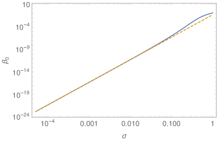
Figure 1: Production probability $\beta_{0}$ in a model of Ref. Har16 . The blue solid line corresponds to the result of the numerical integration of Eq. (29), and the orange dashed line corresponds to the analytic estimate of Eq. (30) for $\sigma\ll 1$.

Using the similar technique of Ref. Har16 , one can obtain analytic estimates for $b^{\mathrm{L}}_{1}$, $b^{\mathrm{L}}_{2}$, and $\omega^{\mathrm{L}}_{1}$ given by Eqs. (82)–(84) for $\sigma\ll 1$. The details of the derivation are given in Appendix B. The results are

$$b^{\mathrm{L}}_{1} \simeq\frac{2^{8}\sqrt{2}}{3^{2}\cdot 7\sqrt{\pi}\,\sigma}\simeq\frac{3.242}{\sigma},$$ (35)

$$b^{\mathrm{L}}_{2} \simeq\frac{10}{\sigma^{2}},$$ (36)

$$\omega^{\mathrm{L}}_{1} \simeq-\frac{5}{2\sigma^{2}}.$$ (37)

Comparing these expressions with Fig. 9 in Appendix B, the power-law behaviors of the bias coefficients for $\sigma\lesssim 0.1$ are accurately explained by the above asymptotic formula.

III.3 Initial PBH power spectrum with primordial non-Gaussianity

Equations (33) and (34) are the renormalized bias functions that we need for evaluating the effects of primordial non-Gaussianity in the initial PBH power spectrum at the lowest order. From Eq. (34), we have $c_{2}(\bm{p},-\bm{p})=(b^{\mathrm{L}}_{2}+2\omega^{\mathrm{L}}_{1})W^{2}(pR)$. Substituting this form into Eq. (12), the integral $C_{2}$ is calculated to be

$$C_{2}=\left(b^{\mathrm{L}}_{2}+2\omega^{\mathrm{L}}_{1}\right)\sigma^{2}.$$ (38)

Thereby, Eq. (11) reduces to

$$P_{\mathrm{PBH}}(k)\simeq\tau_{\mathrm{NL}}\left(b^{\mathrm{L}}_{2}+2\omega^{\mathrm{L}}_{1}\right)^{2}\sigma^{4}\frac{P_{\mathrm{L}}(k)}{\mathcal{M}^{2}(k)}.$$ (39)

This is a main result of this paper.

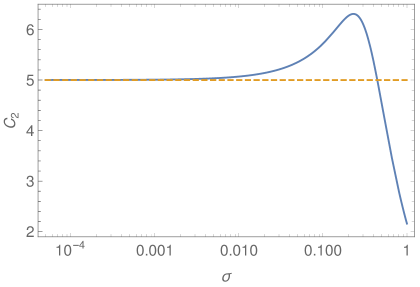
Figure 2: The integral $C_{2}$ of Eq. (38) in the model of Ref. Har16 . Blue solid line: the result of the numerical integrations. Orange dashed line: asymptotic formula $C_{2}=5$ for $\sigma\ll 1$.

In Fig. 2, the result of the numerical integrations for $C_{2}$ (without effects of angular momentum) is plotted. In the case of $\sigma\ll 1$, substituting Eqs. (36) and (37) into Eq. (38) gives $C_{2}\simeq 5$, and we have

$$P_{\mathrm{PBH}}(k)\simeq 25\tau_{\mathrm{NL}}\frac{P_{\mathrm{L}}(k)}{\mathcal{M}^{2}(k)}=25\tau_{\mathrm{NL}}P_{\mathcal{R}}(k).$$ (40)

Interestingly, the analytic estimate of Eq. (40) corresponds to the formula of high-peak limit, Eq. (24) with $\nu=\sqrt{5}$. However this does not imply the PBH formation at the MD epoch corresponds to the density peaks of this height because $b^{\mathrm{L}}_{1}\neq\sqrt{5}/\sigma$. The asymptotic formula of Eq. (40) is accurately applicable for $\sigma\lesssim 0.01$, as one can see from Fig. 2. If only the 10% accuracy is required, the same formula is applicable for $\sigma\lesssim 0.1$.

III.4 Effects of angular momentum

In Ref. Har17 , the model of Ref. Har16 is extended to include the effect of rotation, which turns out to play important roles in the formation of PBHs. The effect of angular momentum in the formation of PBH in the MD epoch exponentially suppresses the amplitude of $\beta_{0}$ for small values of $\sigma$ Har17 . According to Ref. Har17 , the effect of the angular momentum can be taken into account by changing the number density of PBH of Eq. (28) to

$$n_{\mathrm{PBH}}(\alpha,\beta,\gamma)\\ =\frac{\bar{n}_{\mathrm{PBH}}}{\beta_{0}^{\prime}}\Theta(\alpha)\Theta\left(\alpha+\beta+\gamma-\delta_{\mathrm{th}}\right)\Theta\left[1-h(\alpha,\beta,\gamma)\right],$$ (41)

where

$$\beta_{0}^{\prime}=\int_{0}^{\infty}d\alpha\int_{-\infty}^{\alpha}d\beta\int_{-\infty}^{\beta}d\gamma\Theta\left(\alpha+\beta+\gamma-\delta_{\mathrm{th}}\right)\\ \times\Theta\left[1-h(\alpha,\beta,\gamma)\right]w(\alpha,\beta,\gamma),$$ (42)

and $\delta_{\mathrm{th}}$ is the density threshold above which the Kerr bound $L\leq GM^{2}/c$ is satisfied, where $L$ and $M$ are the angular momentum and mass of the black hole, respectively. This bound is required in order to have a black hole at the center of the Kerr metric.

There is an ambiguity in the model on initial quadrupole moment of the mass, which is parametrized by $q$ in Ref. Har17 . There are two cases which are considered in this reference,

$$\delta_{\mathrm{th(1)}}\equiv\frac{12}{125}q^{2},\quad\delta_{\mathrm{th(2)}}\equiv\left(\frac{2}{5}\mathcal{I}\sigma\right)^{2/3},$$ (43)

where $\mathcal{I}$ is another parameter of order unity which characterizes the variance of angular momentum (see Ref. Har17 for explicit definitions of parameters $q$ and $\mathcal{I}$). In the following calculation, we assume $q=\sqrt{2}$ and $\mathcal{I}=1$ to match Fig. 5 of Ref. Har17 . We ignore the effect of the finite duration of the MD epoch. The two thresholds, $\delta_{\mathrm{th(1)}}$ and $\delta_{\mathrm{th(2)}}$, are called first and second order, respectively. In Ref. Har17 , it is suggested that the second-order case is relatively realistic in practice. In Eqs. (41) and (42), the extra factor $\Theta(\alpha+\beta+\gamma-\delta_{\mathrm{th}})$ is inserted in the integrals of Eqs. (28) and (29). The numerical calculations of the bias parameters $b^{\mathrm{L}}_{1}$, $b^{\mathrm{L}}_{2}$ and $\omega^{\mathrm{L}}_{1}$ are similarly possible as in the case of previous subsections. In practice, the function $z_{*}(t,u)$ in Eqs. (89) and (91) is substituted by $z_{*}(t,u)\rightarrow z_{0}(t,u)\equiv\mathrm{max}[z_{*}(t,u),z_{\mathrm{th}}(t)]$, where $z_{\mathrm{th}}\equiv\delta_{\mathrm{th}}/(3t)$.

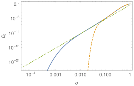
Figure 3: The production probability of PBH with effects of angular momentum in the model of Ref. Har17 . Blue solid line: second-order case with $\delta_{\mathrm{th(2)}}$. Orange dashed line: first-order case with $\delta_{\mathrm{th(1)}}$. Green dotted line: the asymptotic formula of $\sigma\ll 1$ without the effects of angular momentum.

In Fig. 3, the production probability of PBH with effects of angular momentum is plotted. This figure reproduces the corresponding result of Fig. 5 of Ref. Har17 . The second-order case is approximately described by the asymptotic formula without the effects of angular momentum in $0.005\lesssim\sigma\lesssim 0.1$.

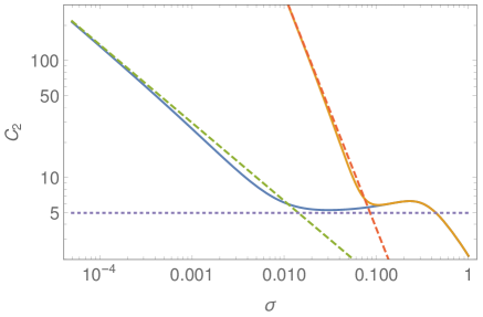
Figure 4: The integral $C_{2}$ of Eq. (38) in the model of Ref. Har17 . Blue solid line: the result of the numerical integrations in the second-order case. Green dashed line: asymptotic formula for $\sigma\ll 1$ in the second-order case. Orange solid line: the result in the first-order case. Orange dashed line: asymptotic formula for $\sigma\ll 1$ in the first-order case. Purple dotted line: asymptotic formula $C_{2}=5$ for $\sigma\ll 1$ without the effects of angular momentum.

In Fig. 4, the result of the numerical integrations for $C_{2}$ with the effects of angular momentum is plotted. Comparing it with Fig. 2, the effects of angular momentum are significant in $\sigma\lesssim 0.01$ for the second-order case and $\sigma\lesssim 0.1$ for the first-order case. Substituting the calculated values of $C_{2}$ into Eq. (11), we obtain the estimate of $P_{\mathrm{PBH}}(k)$ with the effects of angular momentum.

The behaviors of the parameters $b^{\mathrm{L}}_{1}$, $b^{\mathrm{L}}_{2}$, and $\omega^{\mathrm{L}}_{1}$ in $\sigma\ll\delta_{\mathrm{th}}\ll 1$ can also be explained by considering the asymptotic limit of the integrals. They are given in the second subsection of Appendix B, and the results are

$$b^{\mathrm{L}}_{1} \simeq\frac{\delta_{\mathrm{th}}}{\sigma^{2}},$$ (44)

$$b^{\mathrm{L}}_{2} \simeq\frac{{\delta_{\mathrm{th}}}^{2}}{\sigma^{4}},$$ (45)

$$\omega^{\mathrm{L}}_{1} \simeq 0.03400\frac{{\delta_{\mathrm{th}}}^{4}}{\sigma^{4}}-\frac{5}{2\sigma^{2}}.$$ (46)

These asymptotic formulas explain the results of numerical integration for $\sigma\ll 1$ fairly well. From the above, Eq. (38) in the limit of $\sigma\ll\delta_{\mathrm{th}}\ll 1$ is dominated by $b^{\mathrm{L}}_{2}$ and is given by

$$C_{2}\simeq\frac{{\delta_{\mathrm{th}}}^{2}}{\sigma^{2}}.$$ (47)

In the regime where the above approximation applies, we have

$$P_{\mathrm{PBH}}(k)\simeq\tau_{\mathrm{NL}}\left(\frac{\delta_{\mathrm{th}}}{\sigma}\right)^{4}\frac{P_{\mathrm{L}}(k)}{\mathcal{M}^{2}(k)}=\tau_{\mathrm{NL}}\left(\frac{\delta_{\mathrm{th}}}{\sigma}\right)^{4}P_{\mathcal{R}}(k).$$ (48)

Identifying $\delta_{\rm th}/\sigma=\nu$, the above expression is similar to the formula of the high-peak limit, Eq. (24), although $\delta_{\mathrm{th}}$ generally depends on $\sigma$ in this case.

One should note that the production probability $\beta_{0}$ is exponentially suppressed in this regime, and the number density of PBHs is extremely small when the above approximation applies. In fact, $\beta_{0}$ is required to be roughly $\mathcal{O}(10^{-15})$–$\mathcal{O}(10^{-10})$ depending on the mass of PBHs Carr:2009jm in order for PBHs to be a relevant component in dark matter (DM). As can be seen in Fig. 5 in the second-order case (blue solid line), $C_{2}$ is about $5$–$10$ for the above range of production probability $\beta_{0}$. As we have mentioned above, there is an ambiguity for taking the effect of the angular momentum into account. Since the PBH power spectrum is proportional to ${C_{2}}^{2}$, we consider $C_{2}=5$ for the PBHs formed in the MD epoch as a conservative value for the amplitude of the power spectrum in the following discussion. More precise discussion is given in Appendix C, taking into account the dependence of $C_{2}$ on $\sigma$ (or equivalently on $\beta_{0}$).

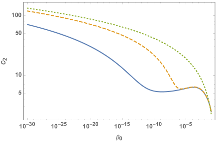
Figure 5: The integral $C_{2}$ of Eq. (38) in the model of Ref. Har17 as a function of $\beta_{0}$. The blue solid line is for the second-order case. The orange dashed line corresponds to the first-order case. The green dotted line represents the case for the PBH formation in the RD epoch calculated by Eqs. (20) and (22).

IV Observational implications

In the previous sections, we obtained the theoretical power spectrum of PBHs which is formed in a MD epoch in the presence of local-type non-Gaussianity. Whether or not this signal has any observable effect is another issue, which we consider in this section. We first estimate the effect of shot noise for possible candidates of PBHs which are connected to observations. Next, we consider the isocurvature fluctuations produced by the PBHs, which can place constraints on the model by comparing with observations of the CMB.

IV.1 Shot-noise contribution

When the produced number of PBHs is too small, their actual power spectrum does not necessarily follow the theoretical prediction because of randomness in the position of each object, or the Poisson shot noise effect. Before we conclude the PBH power spectrum estimated in the previous section is physically meaningful, we have to compare them with the power spectrum of shot noise. The shot-noise contribution to the power spectrum is given by

$$P_{\mathrm{SN}}(k)=\frac{1}{\bar{n}_{\mathrm{PBH}}},$$ (49)

where $\bar{n}_{\text{PBH}}$ is the mean number density of PBHs estimated to be

$$\bar{n}_{\text{PBH}} =\frac{3H_{0}^{2}}{8\pi G}\Omega_{\text{CDM}}\frac{f_{\text{PBH}}}{M_{\text{PBH}}}$$

$$=3\times 10^{22}\,\textrm{Mpc}^{-3}\left(\frac{\Omega_{\text{CDM}}h^{2}}{0.12}\right)\left(\frac{f_{\text{PBH}}}{1}\right)\left(\frac{M_{\text{PBH}}}{10^{-12}M_{\odot}}\right)^{-1}.$$ (50)

Here $H_{0}=100\,h\,\textrm{km/s/Mpc}$ is the Hubble constant, $\Omega_{\text{CDM}}$ is the energy density fraction of cold dark matter, $f_{\mathrm{PBH}}$ is the relative ratio of the energy density of PBHs to those of total dark matter, and $M_{\text{PBH}}$ is the mass of PBHs. Thus, the shot-noise contribution can be expressed in terms of $f_{\rm PBH}$ and $M_{\rm PBH}$, as

$$P_{\text{SN}} =3\times 10^{-23}\,\textrm{Mpc}^{3}\left(\frac{\Omega_{\text{CDM}}h^{2}}{0.12}\right)^{-1}\left(\frac{f_{\text{PBH}}}{1}\right)^{-1}\left(\frac{M_{\text{PBH}}}{10^{-12}M_{\odot}}\right).$$ (51)

Note that the magnitude of the shot noise is determined by the combination $M_{\text{PBH}}/f_{\text{PBH}}$. This contribution behaves as matter isocurvature fluctuations with blue tilt in terms of dimensionless power spectrum $\mathcal{P}(k)\equiv k^{3}P(k)/(2\pi^{2})$, and it would affect the formation of structures on small scales. Based on this fact, one can place a constraint on the abundance $f_{\rm PBH}$ of PBHs by using observations of structures on small scales, such as Lyman-$\alpha$ forest Afshordi:2003zb and future 21cm observations Gong:2017sie .

In Fig. 6, the shot-noise contributions given by Eq. (51) are compared with initial PBH power spectra with the primordial non-Gaussianity given by Eq. (40). Even though the assumed value $C_{2}=5$ corresponds to the asymptotic value without the effects of angular momentum, this gives the lower limit of the power spectrum with the effects of angular momentum, since $C_{2}>5$ in the latter case. Here we assume $\mathcal{P}_{\mathcal{R}}(k)=A_{\mathrm{s}}k^{n_{\mathrm{s}}-1}$ with $A_{\mathrm{s}}=2.101\times 10^{-9}$ and $n_{\mathrm{s}}=0.9649$ Akrami:2018odb for $k\lesssim 10^{3}$ Mpc^-1. The initial PBH power spectrum only depends on the value of $\tau_{\rm NL}$ as seen from Eq. (40). In this figure, we show the power spectrum with multiple choices of $\tau_{\text{NL}}=10^{2}\text{ (purple) },10^{-1}\text{ (blue) },\text{ and }10^{-4}\text{ (dark cyan) }$. For the shot-noise contributions, we consider typical values of $M_{\text{PBH}}/f_{\text{PBH}}=10^{-12}M_{\odot}$, $10^{-3}M_{\odot}$, $10^{4.5}M_{\odot}$, and $10^{10}M_{\odot}$. These values correspond to the cases of all the dark matter (DM: light green, $M_{\rm PBH}=10^{-12}M_{\odot}$, $f_{\rm PBH}=1$) Bartolo:2018rku , excess events of OGLE observations (OGLE: dark yellow, $M_{\rm PBH}=10^{-5}M_{\odot}$, $f_{\rm PBH}=10^{-2}$) Niikura:2019kqi ; Tada:2019amh ; Fu:2019ttf , the origin of binary black holes leading to the gravitational-wave events of LIGO/Virgo (LIGO/Virgo: orange, $M_{\rm PBH}=10^{1.5}M_{\odot}$, $f_{\rm PBH}=10^{-3}$) Bird:2016dcv ; Sasaki:2016jop ; Sasaki:2018dmp , and the seeds of supermassive black holes (SMBH: red, $M_{\rm PBH}=10^{3.5}M_{\odot}$, $f_{\rm PBH}=10^{-6.5}$) Kawasaki:2012kn ; Kohri2014SMBH ; Kawasaki:2019iis , respectively. These are just benchmark points, and the actual allowed region of $M_{\mathrm{PBH}}$ is not a point but a band. Also, the favored region for $M_{\text{PBH}}$ and $f_{\text{PBH}}$ has a large uncertainty. However, we are not particularly interested in these issues here.

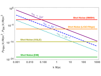
Figure 6: Comparison of the initial PBH power spectrum induced by primordial non-Gaussianity during the MD epoch [Eq. (40)] (oblique lines) with the shot noise contribution [Eq. (51)] (horizontal lines) as a function of wave number $k$. The assumed typical values of $M_{\text{PBH}}/(M_{\odot}f_{\text{PBH}})$ for DM, OGLE, LIGO/Virgo, and SMBH are $10^{-12}$, $10^{-3}$, $10^{4.5}$, and $10^{10}$, respectively. Note that the SMBH case is irrelevant for PBH production in a MD epoch, but it is nevertheless shown because the figure is applicable to the case of the RD epoch (high-peak limit) by the replacement of the normalization of the oblique lines, $25\to\nu^{4}$.

Note also that for the PBH production in the early MD epoch, the SMBH case requires a reheating temperature too low to be consistent with big bang nucleosynthesis Hasegawa:2019jsa (see also Refs. Kawasaki:1999na ; Kawasaki:2000en ; Hannestad:2004px ; Ichikawa:2005vw ; deSalas:2015glj ). The reason why we nevertheless show the typical line corresponding to this case in Fig. 6 is because these results are also applicable to the case of PBH production in the RD epoch after making the replacement $25\to\nu^{4}$ for the magnitude of the PBH power spectrum (the high-peak limit is assumed). When the mass of PBHs is less than $10^{7}\,M_{\odot}$, the threshold value for the production of PBHs in the RD epoch is given by $\nu^{4}\gtrsim 400$ TY15 . In this case, the amplitude of the PBH power spectrum in Fig. 6 is 16 times larger than the plotted lines.

In Fig. 6, we see that the shot-noise contribution becomes relatively unimportant on large scales because of the scale dependence of the initial PBH power spectrum approximately $k^{n_{\mathrm{s}}-3}$. Also, for DM or OGLE, the shot noise is completely negligible for the scales of CMB and the large-scale structure.

IV.2 Constraints from isocurvature mode in CMB

The initial clustering of primordial black holes induced from the primordial non-Gaussianity would be observed as isocurvature perturbations. The isocurvature perturbations are well constrained by CMB, and thus the abundance of PBHs $f_{\mathrm{PBH}}$ or the magnitude of $\tau_{\mathrm{NL}}$ is constrained as well.

The PBH isocurvature perturbations are given by

$$\mathcal{I}_{\rm PBH}=\delta_{\mathrm{PBH}}-\frac{\delta}{1+w},$$ (52)

where $\delta_{\mathrm{PBH}}$ is the density contrast of PBHs, $\delta$ is the density contrast of the dominant component of the Universe which turns into the radiation component in the RD epoch, and $w$ is the equation-of-state parameter of the latter component. On comoving slices, from Eq. (6), the density contrast of the dominant component of the Universe must be much suppressed by $k^{2}$ in $\mathcal{M}(k)$ in the large-scale limit. Here, we consider the PBH isocurvature perturbations at CMB scales which are much larger than the PBH formation scale, and hence the PBH isocurvature perturbations are simply given by $\mathcal{I}_{\rm PBH}=\delta_{\mathrm{PBH}}$ where $\delta$ is negligible on large scales.

The Planck Collaboration gives a constraint on the total CDM isocurvature perturbations, and thus, if the PBHs exist as a DM component with the fraction, $f_{\rm PBH}$, the power spectrum of the total CDM isocurvature perturbations can be given as

$$P_{\mathcal{I}\mathcal{I}}(k)=f_{\mathrm{PBH}}^{2}P_{\mathrm{PBH}}(k),$$ (53)

where we have assumed that the other DM components do not have any isocurvature perturbations. Substituting Eq. (11) into the above expression, the power spectrum of CDM isocurvature perturbation is given by

$$P_{\mathcal{I}\mathcal{I}}(k)={C_{2}}^{2}{f_{\mathrm{PBH}}}^{2}\tau_{\mathrm{NL}}P_{\mathcal{R}}(k).$$ (54)

The above equation holds for PBH formation in both the RD ($C_{2}=\nu^{2}$) TY15 and MD ($C_{2}\geq 5$) epochs.

The constraint on the CDM isocurvature perturbations (for correlated case) placed by Planck 2018 Akrami:2018odb is given by $P_{\mathcal{II}}/P_{\mathcal{R}}\lesssim 10^{-3}$ on CMB scales. Applying this constraint to our result, we obtain an upper bound on $f_{\text{PBH}}$ depending on the value of $\tau_{\rm NL}$ as follows:

$$f_{\text{PBH}}<\frac{3\times 10^{-2}}{C_{2}\sqrt{\tau_{\text{NL}}}}.$$ (55)

In the limit of $\tau_{\text{NL}}\to 0$, the isocurvature upper bound on $f_{\text{PBH}}$ disappears, which is consistent with the understanding that it is non-Gaussianity that induces the PBH isocurvature perturbations.

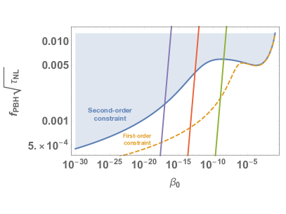
Figure 7: Upper bounds on $f_{\text{PBH}}\sqrt{\tau_{\text{NL}}}$ as a function of $\beta_{0}$ in the case of PBH production in a MD epoch by the second-order mechanism (blue solid line) and by the first-order mechanism (orange dashed line). Three examples of $f_{\text{PBH}}\sqrt{\tau_{\text{NL}}}$ are plotted as functions of $\beta_{0}$: $T_{\text{R}}=10^{-2}$ GeV (Green line), $10^{2}$ GeV (red line), and $10^{6}$ GeV (purple line) with $\tau_{\text{NL}}=10^{-2}$ for all cases.

The above constraint can be rewritten as $f_{\text{PBH}}\sqrt{\tau_{\text{NL}}}<3\times 10^{-2}/C_{2}$, which is an upper bound on the combination $f_{\text{PBH}}\sqrt{\tau_{\text{NL}}}$ given the value of $C_{2}$, which in turn depends on $\beta_{0}$. This is shown in Fig. 7 in the case of PBH production in a MD epoch. The shaded region is excluded by the isocurvature constraint (the blue line corresponding to the second-order case). The first-order constraint is also shown by the orange dashed line. Actually, $f_{\text{PBH}}$ (present abundance) itself depends linearly on $\beta_{0}$ (initial abundance) (see, e.g., Refs. Inomata:2016rbd ; Kohri:2018qtx ),

$$f_{\text{PBH}} \equiv\frac{\rho_{\text{PBH}}}{\rho_{\text{CDM}}}$$

$$=\frac{g_{*}(T)g_{*,s}(T_{\text{eq}})T}{g_{*}(T_{\text{eq}})g_{*,s}(T)T_{\text{eq}}}\gamma\beta_{0}\frac{\Omega_{\text{m}}}{\Omega_{\text{CDM}}},$$ (56)

where $g_{*}(T)$ and $g_{*,s}(T)$ are the effective relativistic degrees of freedom for energy density and entropy, respectively; $T_{\text{eq}}$ is the temperature at the matter-radiation equality; $\gamma$ ($\approx 0.2$ in the RD epoch Carr:1975qj ) is an efficiency parameter parametrizing how much fraction of the horizon mass goes into the PBH; and $\Omega_{\text{m}}$ is the energy density fraction of total matter. The above expression should be evaluated at the temperature when the scale that becomes PBHs enters the horizon in the case of PBH production in the RD epoch or at the reheating temperature in the case of PBH production in the early MD epoch Carr:2017edp ; Kohri:2018qtx . The efficiency parameter in the early MD epoch has some uncertainty, and we assume $\gamma=1$ following Ref. Kohri:2018qtx . Using this relation, example lines of $f_{\text{PBH}}\sqrt{\tau_{\text{NL}}}$ are shown in the same figure for $T_{\text{R}}=10^{-2}$ GeV (green line), $10^{2}$ GeV (red line), and $10^{6}$ GeV (purple line) with $\tau_{\text{NL}}=10^{-2}$. The intersection of such a line and the constraint curve gives the upper bound on $f_{\text{PBH}}$ given the values of $T_{\text{R}}$ and $\tau_{\text{NL}}$. These lines are drawn from numerical solutions as explained in Appendix C.

Unless $\sigma$ is too large, the value of $C_{2}$ is always larger than $5$ regardless of uncertainty in estimating the effect of angular momentum. In the case of PBH formation in the RD epoch, the value of $C_{2}$ is much larger than $5$. Therefore, one can conclude that the bound $C_{2}\geq 5$ is conservatively satisfied in the PBH formation in both the RD and MD epochs. Combining this bound with Eq. (55), we have a conservative upper bound,

$$f_{\mathrm{PBH}}\sqrt{\tau_{\mathrm{NL}}}<6\times 10^{-3}.$$ (57)

If we only consider the PBH formation in the RD epoch, $C_{2}\gtrsim 20$, the upper bound becomes smaller, $f_{\mathrm{PBH}}\sqrt{\tau_{\mathrm{NL}}}<2\times 10^{-3}$. In either case, the order of magnitude of the upper bounds is not significantly different.

It is remarkable that the possibility of PBHs being all of the dark matter ($f_{\mathrm{PBH}}=1$) can be excluded by the isocurvature constraint for $\tau_{\text{NL}}\gtrsim 4\times 10^{-5}$ (MD, $C_{2}\geq 5$) and $\tau_{\text{NL}}\gtrsim 3\times 10^{-6}$ (RD, $C_{2}\gtrsim 20$). In other words, the hypothesis of all the dark matter places a conservative upper bound on $\tau_{\text{NL}}$, irrespective of the formation epoch,

$$\tau_{\text{NL}}<4\times 10^{-5} (100\%~{}\text{PBH dark matter}).$$ (58)

V Conclusions

In this paper, we derive a general prediction of the initial clustering of PBHs in the presence of the parameter $\tau_{\mathrm{NL}}$ of local-type primordial non-Gaussianity. Using the formalism of iPT, we generally have Eq. (11), which is the prediction of the large-scale power spectrum in the presence of $\tau_{\mathrm{NL}}$. In the case of PBHs, the result is given by $P_{\mathrm{PBH}}(k)\simeq\tau_{\mathrm{NL}}{C_{2}}^{2}P_{\mathcal{R}}(k)$ for $k\ll R^{-1}$, where $R$ is the initial radius of proto-PBHs with mass $M\sim 4\pi R^{3}/3$ up to the efficiency parameter. Evaluating the integral $C_{2}$ in the high-peak limit, the linear power spectrum of PBH formed in the RD epoch is given by Eq. (24), which is consistent to the previous work TY15 ; SY19 . In the case of PBHs formed in a MD epoch, we adopt a model of Refs. Har16 ; Har17 and evaluate the initial power spectrum of PBHs.

The integral $C_{2}$ is a decisive factor for the amplitude of initial clustering of PBHs in the presence of $\tau_{\mathrm{NL}}$. For the thresholded regions, it is given by $C_{2}=H_{1}(\nu)/H_{-1}(\nu)$, and this result reduces to $C_{2}=\nu^{2}$ in the high-peak limit $\nu\gg 1$. In the case of PBHs formed in a MD epoch, the integral can be numerically evaluated. In the regime where the effects of angular momentum are neglected, we have an analytic estimate $C_{2}\simeq 5$ for $\sigma\ll 1$. In the regime where the angular momentum is important, we have another analytic estimate $C_{2}\simeq(\delta_{\mathrm{th}}/\sigma)^{2}$, where $\delta_{\mathrm{th}}$ is given by Eq. (43). In general, one can evaluate the value of $C_{2}$ by numerical integrations. The results are given in Figs. 2 and 4 without and with effects of angular momentum, respectively.

Because of the approximately $k^{n_{\mathrm{s}}-4}\sim k^{-3}$ scaling of the PBH power spectrum from the primordial non-Gaussianity, the shot-noise contributions are relatively unimportant on large scales, unless the mass of PBHs is extremely large and the number density of PBHs is extremely small.

The clustering of PBHs produces the isocurvature perturbations in the early Universe. The isocurvature power spectrum is proportional to ${C_{2}}^{2}{f_{\mathrm{PBH}}}^{2}\tau_{\mathrm{NL}}$. Putting $C_{5}=5$ as a conservative value, the current constraint by the Planck satellite gives an upper bound, $f_{\mathrm{PBH}}\sqrt{\tau_{\mathrm{NL}}}<6\times 10^{-3}$. On one hand, unless the non-Gaussianity parameter $\tau_{\mathrm{NL}}$ is smaller than approximately $4\times 10^{-5}$, the hypothesis that all the dark matter is made of PBHs is excluded. On the other hand, if all the dark matter is made of PBHs, the parameter $\tau_{\mathrm{NL}}$ of the primordial non-Gaussianity should be smaller than $4\times 10^{-4}$.

Appendix A Derivation of renormalized bias functions

In this Appendix, we derive the renormalized bias functions $c_{1}$ and $c_{2}$ in our model of the number density $n_{\mathrm{PBH}}$. This number density $n_{\mathrm{PBH}}$ is a function of a finite number of variables, $\varphi_{ij}$. In this case, the renormalized bias function of Eq. (31) reduces to Mat11

$$c_{n}(\bm{k}_{1},\ldots,\bm{k}_{n})=\frac{1}{\bar{n}_{\mathrm{PBH}}}\sum_{a_{1},\ldots,a_{n}}\left\langle\frac{\partial^{n}n_{\mathrm{PBH}}}{\partial y_{a_{1}}\cdots\partial y_{a_{n}}}\right\rangle U_{a_{1}}(\bm{k}_{1})\cdots U_{a_{n}}(\bm{k}_{n}),$$ (59)

where

$$\left(y_{a}\right) =\left(\varphi_{11},\varphi_{22},\varphi_{33},\varphi_{12},\varphi_{23},\varphi_{13}\right),$$ (60)

$$\left(U_{a}\right) =W(kR)\left({\hat{k}_{1}}^{2},{\hat{k}_{2}}^{2},{\hat{k}_{3}}^{2},\hat{k}_{1}\hat{k}_{2},\hat{k}_{2}\hat{k}_{3},\hat{k}_{1}\hat{k}_{3}\right),$$ (61)

and $\hat{k}_{i}=k_{i}/k$ is the $i\mathrm{th}$ component of $\bm{k}/k$. With the above definition, we have a relation, $y_{a}(\bm{k})=U_{a}(\bm{k})\delta_{\mathrm{L}}(\bm{k})$. We define an operator,

$$\mathcal{D}(\bm{k})\equiv W(kR)\hat{k}_{i}\hat{k}_{j}\frac{\partial}{\partial\varphi_{ij}},$$ (62)

where repeated indices are summed over, and partial derivatives are taken as if $\varphi_{ij}$ and $\varphi_{ji}$ are independent variables (because of the reason described in Ref. MD16 , $n_{\mathrm{PBH}}$ can contain $\varphi_{ji}$ with $i>j$, provided that $\varphi_{ji}=\varphi_{ij}$). With this operator, Eq. (59) reduces to MD16

$$c_{n}(\bm{k}_{1},\ldots,\bm{k}_{n})=\frac{1}{\bar{n}_{\mathrm{PBH}}}\left\langle\mathcal{D}(\bm{k}_{1})\cdots\mathcal{D}(\bm{k}_{n})n_{\mathrm{PBH}}\right\rangle=\frac{(-1)^{n}}{\bar{n}_{\mathrm{PBH}}}\int d^{6}\!y\,n_{\mathrm{PBH}}(\bm{y})\mathcal{D}(\bm{k}_{1})\cdots\mathcal{D}(\bm{k}_{n})\mathcal{P}(\bm{y}),$$ (63)

where $\mathcal{P}(\bm{y})$ is a joint probability distribution function of $\bm{y}=(y_{a})$.

In the presence of initial non-Gaussianity, the probability distribution function $\mathcal{P}$ is not strictly multivariate Gaussian. However, as the lowest-order non-Gaussianity is concerned in Eq. (11), it is sufficient to use the renormalized bias function derived from the Gaussian distribution function. Evaluation of the renormalized bias functions of Eq. (63) can be performed in a method similar to that developed in Ref. MD16 . The Gaussian distribution function is given by

$$\mathcal{P}(\bm{y})=\frac{1}{\sqrt{(2\pi)^{6}\det\mathcal{M}}}\exp\left(-\frac{1}{2}\bm{y}^{\mathrm{T}}\mathcal{M}^{-1}\bm{y}\right),$$ (64)

where

$$\mathcal{M}_{ab}=\left\langle y_{a}y_{b}\right\rangle=\int\frac{d^{3}\!k}{(2\pi)^{3}}U_{a}^{*}(\bm{k})U_{b}(\bm{k})P_{\mathrm{L}}(k),$$ (65)

is the covariance matrix, and $P_{\mathrm{L}}(k)$ is the linear power spectrum of the density perturbations. The elements of the covariance matrix are given by

$$\left\langle\varphi_{ij}\varphi_{kl}\right\rangle=\int\frac{d^{3}\!k}{(2\pi)^{3}}\hat{k}_{i}\hat{k}_{j}\hat{k}_{k}\hat{k}_{l}W^{2}(kR)P_{\mathrm{L}}(k)=\frac{\sigma^{2}}{15}\left(\delta_{ij}\delta_{kl}+\delta_{ik}\delta_{jl}+\delta_{il}\delta_{jk}\right).$$ (66)

The joint probability distribution function $\mathcal{P}(\bm{y})$ depends only on rotationally invariant quantities PGP09 ; GPP12 . They are

$$J_{1}\equiv\frac{1}{\sigma}\varphi_{ii},\quad J_{2}\equiv\frac{3}{2\sigma^{2}}\tilde{\varphi}_{ij}\tilde{\varphi}_{ji},\quad J_{3}=\frac{9}{2\sigma^{3}}\tilde{\varphi}_{ij}\tilde{\varphi}_{jk}\tilde{\varphi}_{ki},$$ (67)

where

$$\tilde{\varphi}_{ij}\equiv\varphi_{ij}-\frac{\sigma}{3}\delta_{ij}J_{1},$$ (68)

is the traceless part of $\varphi_{ij}$. With the invariant variables of Eq. (67), the distribution function of Eq. (64) reduces to GPP12

$$\mathcal{P}(\bm{y})\propto\exp\left(-\frac{1}{2}{J_{1}}^{2}-\frac{5}{2}J_{2}\right),$$ (69)

up to the normalization factor.

Using relations,

$$\frac{\partial J_{1}}{\partial\varphi_{ij}}=\frac{1}{\sigma}\delta_{ij},\quad\frac{\partial J_{2}}{\partial\varphi_{ij}}=\frac{3}{\sigma^{2}}\tilde{\varphi}_{ji},\quad\frac{\partial\tilde{\varphi}_{kl}}{\partial\varphi_{ij}}=\delta_{ik}\delta_{jl}-\frac{1}{3}\delta_{ij}\delta_{kl},$$ (70)

the second-order derivatives are given by

$$\frac{\partial}{\partial\varphi_{ij}}\mathcal{P} =\left[\frac{\delta_{ij}}{\sigma}\frac{\partial}{\partial J_{1}}+\frac{3\tilde{\varphi}_{ij}}{\sigma^{2}}\frac{\partial}{\partial J_{2}}\right]\mathcal{P},$$ (71)

$$\frac{\partial^{2}}{\partial\varphi_{ij}\partial\varphi_{kl}}\mathcal{P} =\left[\frac{\delta_{ij}\delta_{kl}}{\sigma^{2}}\frac{\partial^{2}}{\partial{J_{1}}^{2}}-\frac{3}{\sigma^{3}}\left(\delta_{ij}\tilde{\varphi}_{kl}+\delta_{kl}\tilde{\varphi}_{ij}\right)\frac{\partial^{2}}{\partial J_{1}\partial J_{2}}+\frac{9\tilde{\varphi}_{ij}\tilde{\varphi}_{kl}}{\sigma^{4}}\frac{\partial^{2}}{\partial{J_{2}}^{2}}+\frac{3\delta_{ik}\delta_{jl}-\delta_{ij}\delta_{kl}}{\sigma^{2}}\frac{\partial}{\partial J_{2}}\right]\mathcal{P}.$$ (72)

In calculating Eq. (63), one notices that the number density $n_{\mathrm{PBH}}$ and the distribution function $\mathcal{P}$ depend only on rotationally invariant variables. Thus we can first average over the angular dependence in the product of operators $\mathcal{D}(\bm{k})$. Denoting the angular average by $\langle\cdots\rangle_{\Omega}$, Eq. (63) reduces to

$$c_{n}(\bm{k}_{1},\ldots,\bm{k}_{n})=\frac{(-1)^{n}}{\bar{n}_{\mathrm{PBH}}}\int d^{6}\!y\,n_{\mathrm{PBH}}(\bm{y})\left\langle\mathcal{D}(\bm{k}_{1})\cdots\mathcal{D}(\bm{k}_{n})\mathcal{P}(\bm{y})\right\rangle_{\Omega}.$$ (73)

Using relations,

$$\left\langle\tilde{\varphi}_{ij}\right\rangle_{\Omega}=0,\quad\left\langle\tilde{\varphi}_{ij}\tilde{\varphi}_{kl}\right\rangle_{\Omega}=\frac{\sigma^{2}}{15}\left(\delta_{ik}\delta_{jl}+\delta_{il}\delta_{jk}-\frac{2}{3}\delta_{ij}\delta_{kl}\right)J_{2},$$ (74)

the angular averages in the integrand of Eq. (73) for $n=1,2$ are given by

$$\left\langle\mathcal{D}(\bm{k})\mathcal{P}\right\rangle_{\Omega} =\frac{W(kR)}{\sigma}\frac{\partial}{\partial J_{1}}\mathcal{P}=-\frac{W(kR)}{\sigma}J_{1}\mathcal{P},$$ (75)

$$\left\langle\mathcal{D}(\bm{k}_{1})\mathcal{D}(\bm{k}_{2})\mathcal{P}\right\rangle_{\Omega} =\frac{W(k_{1}R)W(k_{2}R)}{\sigma^{2}}\left\{\frac{\partial^{2}}{\partial{J_{1}}^{2}}+\left[3(\hat{\bm{k}}_{1}\cdot\hat{\bm{k}}_{2})^{2}-1\right]\left(1+\frac{2}{5}J_{2}\frac{\partial}{\partial J_{2}}\right)\frac{\partial}{\partial J_{2}}\right\}\mathcal{P}$$

$$=\frac{W(k_{1}R)W(k_{2}R)}{\sigma^{2}}\left\{{J_{1}}^{2}-1+\left[3(\hat{\bm{k}}_{1}\cdot\hat{\bm{k}}_{2})^{2}-1\right]\frac{5}{2}\left(J_{2}-1\right)\right\}\mathcal{P}.$$ (76)

Substituting Eqs. (75) and (A) into Eq. (73), the first- and second-order renormalized bias functions are derived as

$$c_{1}(\bm{k}) =b^{\mathrm{L}}_{1}W(kR),$$ (77)

$$c_{2}(\bm{k}_{1},\bm{k}_{2}) =\left\{b^{\mathrm{L}}_{2}+\left[3(\hat{\bm{k}}_{1}\cdot\hat{\bm{k}}_{2})^{2}-1\right]\omega^{\mathrm{L}}_{1}\right\}W(k_{1}R)W(k_{2}R),$$ (78)

where

$$b^{\mathrm{L}}_{1}\equiv\frac{1}{\sigma\bar{n}_{\mathrm{PBH}}}\left\langle J_{1}n_{\mathrm{PBH}}\right\rangle,\quad b^{\mathrm{L}}_{2}\equiv\frac{1}{\sigma^{2}\bar{n}_{\mathrm{PBH}}}\left\langle\left({J_{1}}^{2}-1\right)n_{\mathrm{PBH}}\right\rangle,\quad\omega^{\mathrm{L}}_{1}\equiv\frac{1}{\sigma^{2}\bar{n}_{\mathrm{PBH}}}\left\langle\frac{5}{2}\left(J_{2}-1\right)n_{\mathrm{PBH}}\right\rangle,$$ (79)

and $\langle\cdots\rangle=\int d^{6}\!y\cdots\mathcal{P}(\bm{y})$. General definitions of $b^{\mathrm{L}}_{n}$ and $\omega^{\mathrm{L}}_{l}$ are given by MD16

$$b^{\mathrm{L}}_{n}\equiv\frac{1}{\sigma^{n}\bar{n}_{\mathrm{PBH}}}\left\langle H_{n}\left(J_{1}\right)n_{\mathrm{PBH}}\right\rangle,\quad\omega_{l}\equiv\frac{(-1)^{l}}{\sigma^{2l}\bar{n}_{\mathrm{PBH}}}\left\langle L^{(3/2)}_{l}\left(\frac{5}{2}J_{2}\right)n_{\mathrm{PBH}}\right\rangle,$$ (80)

where $H_{n}(x)$ is the Hermite polynomial and $L^{(\alpha)}_{l}(x)$ is the generalized Laguerre polynomial.

The variables $J_{1}$ and $J_{2}$, which are defined by Eq. (67), are represented by eigenvalues of $\varphi_{ij}$ as

$$J_{1}(\alpha,\beta,\gamma)=\frac{\alpha+\beta+\gamma}{\sigma},\quad J_{2}(\alpha,\beta,\gamma)=\frac{\alpha^{2}+\beta^{2}+\gamma^{2}-\alpha\beta-\beta\gamma-\gamma\alpha}{\sigma^{2}}.$$ (81)

Using the distribution function $w(\alpha,\beta,\gamma)$ of Eq. (27), Eq. (79) reduces to

$$b^{\mathrm{L}}_{1} \equiv\frac{1}{\sigma\beta_{0}}\int_{0}^{\infty}d\alpha\int_{-\infty}^{\alpha}d\beta\int_{-\infty}^{\beta}d\gamma J_{1}(\alpha,\beta,\gamma)\Theta\left[1-h(\alpha,\beta,\gamma)\right]w(\alpha,\beta,\gamma),$$ (82)

$$b^{\mathrm{L}}_{2} \equiv\frac{1}{\sigma^{2}\beta_{0}}\int_{0}^{\infty}d\alpha\int_{-\infty}^{\alpha}d\beta\int_{-\infty}^{\beta}d\gamma\left[J_{1}(\alpha,\beta,\gamma)\right]^{2}\Theta\left[1-h(\alpha,\beta,\gamma)\right]w(\alpha,\beta,\gamma)-\frac{1}{\sigma^{2}},$$ (83)

$$\omega^{\mathrm{L}}_{1} \equiv\frac{5}{2\sigma^{2}\beta_{0}}\int_{0}^{\infty}d\alpha\int_{-\infty}^{\alpha}d\beta\int_{-\infty}^{\beta}d\gamma J_{2}(\alpha,\beta,\gamma)\Theta\left[1-h(\alpha,\beta,\gamma)\right]w(\alpha,\beta,\gamma)-\frac{5}{2\sigma^{2}}.$$ (84)

Appendix B Analytic estimates of renormalized bias functions

In this Appendix, the three-dimensional integrations of the previous Appendix are reduced to two-dimensional integrals. After that, analytic estimates for the coefficients $b^{\mathrm{L}}_{1}$, $b^{\mathrm{L}}_{2}$, and $\omega^{\mathrm{L}}_{1}$ of Eqs. (82)–(84) are derived in a limit of $\sigma\ll 1$. Analytic estimates with the effects of angular momentum are also presented.

B.1 Without the effects of angular momentum

According to Ref. Har16 , it is useful to define new variables,

$$t=\frac{2}{3}\frac{\alpha+\beta+\gamma}{\alpha-\gamma},\quad u=\frac{1}{2}\frac{\alpha-2\beta+\gamma}{\alpha-\gamma},\quad z=\frac{\alpha-\gamma}{2}.$$ (85)

The domain of integration, $\alpha>\beta>\gamma$, $\alpha>0$ in Eqs. (82)–(84) corresponds to $-1/2<u<1/2$, $t>-(1+2u/3)$ and $z>0$. The condition $h(\alpha,\beta,\gamma)<1$ is equivalent to

$$z>z_{*}(t,u)\equiv\frac{4}{\pi}\left(t+\frac{2}{3}u+1\right)^{-2}E\left[\sqrt{1-\left(u+\frac{1}{2}\right)^{2}}\right].$$ (86)

With new variables, we have

$$w(\alpha,\beta,\gamma)d\alpha\,d\beta\,d\gamma=\frac{3^{3}\cdot 5^{5/2}}{\pi\sigma^{6}}(1+2u)(1-2u)z^{5}e^{-A(t,u)z^{2}}dt\,du\,dz,$$ (87)

where

$$A(t,u)\equiv\frac{1}{\sigma^{2}}\left(\frac{9}{2}t^{2}+10u^{2}+\frac{15}{2}\right).$$ (88)

Defining the integrals,

$$I_{nml}\equiv\int_{-1/2}^{1/2}du(1-2u)(1+2u)u^{n}\int_{-(1+2u/3)}^{\infty}dt\,(3t)^{m}\int_{z_{*}(t,u)}^{\infty}dz\,z^{l+5}e^{-A(t,u)z^{2}},$$ (89)

Eqs. (29) and (82)–(84) reduce to

$$\beta_{0}=\frac{3^{3}\cdot 5^{5/2}}{\pi\,\sigma^{6}}I_{000},\qquad b^{\mathrm{L}}_{1}=\frac{I_{011}}{\sigma^{2}I_{000}},\qquad b^{\mathrm{L}}_{2}=\frac{1}{\sigma^{2}}\left(\frac{I_{022}}{\sigma^{2}I_{000}}-1\right),\qquad\omega^{\mathrm{L}}_{1}=\frac{5}{2\sigma^{2}}\left(\frac{4I_{202}+3I_{002}}{\sigma^{2}I_{000}}-1\right).$$ (90)

These expressions are the exact transformation of the original integrals, Eqs. (29) and (82)–(84), without any approximation. The last integral over $z$ in Eq. (89) can be analytically evaluated as

$$\int_{z_{*}(t,u)}^{\infty}dz\,z^{l+5}e^{-Az^{2}}=A^{-(l+6)/2}\int_{\sqrt{A}z_{*}}^{\infty}dr\,r^{l+5}e^{-r^{2}}=\frac{1}{2}A^{-(l+6)/2}\Gamma\left(\frac{l}{2}+3,A{z_{*}}^{2}\right),$$ (91)

where $\Gamma(x)$ is the gamma function.

Next, we derive the analytic estimates of the integrals of Eq. (89) in a limit $\sigma\ll 1$. In this limit, the integral over $t$ is dominantly contributed by a region $t\gtrsim\sigma^{-1}$, since the contribution from $t\lesssim\sigma^{-1}$ is exponentially suppressed Har16 . Therefore, the dominant contribution comes from $t\gtrsim\sigma^{-1}\gg 1$, and in this region, we have $A\simeq 9t^{2}/(2\sigma^{2})$, $z_{*}\simeq 4E/(\pi t^{2})$, and $A{z_{*}}^{2}\simeq 72E^{2}/(\pi^{2}\sigma^{2}t^{2})$. The lower limit $-(1+2u/3)$ of the integral over $t$ can be replaced by $0$ because $t\gg 1$. Introducing variables $s=6\sqrt{2}E/(\pi\sigma t)$ (with $u$ fixed) and $r=\sqrt{A}z$ (with $t,u$ fixed), the last two integrals in Eq. (89) are approximately given by

$$\int_{-(1+2u/3)}^{\infty}dt\,(3t)^{m}\int_{z_{*}(t,u)}^{\infty}dz\,z^{l+5}e^{-A(t,u)z^{2}}\simeq\frac{(2\sigma^{2})^{l/2+3}}{3^{l-m+6}}\left(\frac{\pi\sigma}{6\sqrt{2}E}\right)^{l-m+5}\int_{0}^{\infty}ds\,s^{l-m+4}\int_{s}^{\infty}dr\,r^{l+5}e^{-r^{2}},$$ (92)

where the argument of the elliptic integral $E$ is the same as in Eq. (86). Using a partial integration, the above integral reduces to an analytic form with a gamma function. As a result, Eq. (89) in the case of $\sigma\ll 1$ is given by

$$I_{nml}\simeq\frac{\Gamma(l-m/2+11/2)}{l-m+5}2^{-l+3m/2-9/2}\cdot 3^{-2l+2m-12}\pi^{l-m+5}\sigma^{2l-m+11}\frac{3}{2}\int_{-1/2}^{1/2}du(1-2u)(1+2u)u^{n}E^{-l+m-5}.$$ (93)

Substituting Eq. (93) into Eq. (90), we have

$$\beta_{0}\simeq\frac{5^{3}\cdot 7\pi^{9/2}}{2^{9}\cdot 3^{6}\sqrt{10}}\bar{E}^{-5}\sigma^{5}\simeq 0.05556\sigma^{5},$$ (94)

where

$$\bar{E}^{-5}\equiv\frac{3}{2}\int_{-1/2}^{1/2}du(1-2u)(1+2u)E^{-5},$$ (95)

which is already known in Ref. Har16 . Substituting Eq. (93) into Eq. (90), we have

$$b^{\mathrm{L}}_{1}\simeq\frac{2^{8}\sqrt{2}}{3^{2}\cdot 7\sqrt{\pi}\sigma}\simeq\frac{3.242}{\sigma},\qquad b^{\mathrm{L}}_{2}\simeq\frac{10}{\sigma^{2}},\qquad\omega^{\mathrm{L}}_{1}\simeq-\frac{5}{2\sigma^{2}},$$ (96)

where only dominant terms of $\sigma\ll 1$ are retained.

In Fig. 9, the bias coefficients $b^{\mathrm{L}}_{1}$, $b^{\mathrm{L}}_{2}$, and $\omega^{\mathrm{L}}_{1}$ as functions of $\sigma$ are plotted. Numerical integrations are performed by Eq. (90) with Eqs. (89) and (91). These coefficients for $\sigma\lesssim 0.1$ have power-law shapes, which are well described by Eq. (96).

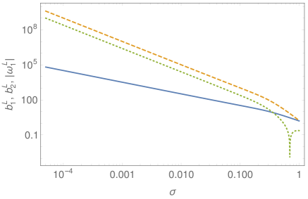
Figure 8: Bias coefficients $b^{\mathrm{L}}_{1}$ (blue solid line), $b^{\mathrm{L}}_{2}$ (orange dashed line), and $\omega^{\mathrm{L}}_{1}$ (green dotted line) in the model of Ref. Har16 . The parameter $\omega^{\mathrm{L}}_{1}$ is negative except for $\sigma\gtrsim 0.65$.

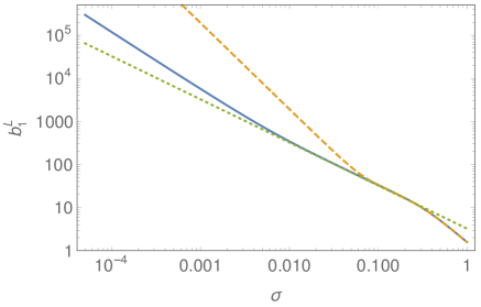
Figure 9: The bias coefficient $b^{\mathrm{L}}_{1}$ for second-order case (blue solid line), first-order case (orange dashed line) and the asymptotic formula of $\sigma\ll 1$ without the effects of angular momentum (green dotted line).

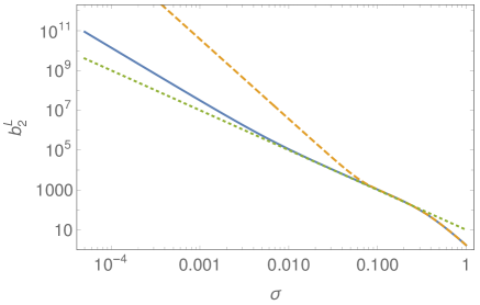
Figure 10: Same as in Fig. 9 but for the bias coefficient $b^{\mathrm{L}}_{2}$.

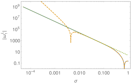
Figure 11: Same as in Fig. 9 but for the bias coefficient $\omega^{\mathrm{L}}_{1}$.

B.2 Effects of angular momentum

We briefly give the analytic estimates including the effects of angular momentum. In this case, the integrands of Eqs. (29) and (82)–(84) are multiplied by a factor, $\Theta(\alpha+\beta+\gamma-\delta_{\mathrm{th}})$. The function $z_{*}(t,u)$ in Eqs. (89) and (91) is substituted by $z_{*}(t,u)\rightarrow z_{0}(t,u)\equiv\mathrm{max}[z_{*}(t,u),z_{\mathrm{th}}(t)]$, where $z_{\mathrm{th}}\equiv\delta_{\mathrm{th}}/(3t)$. Extending the derivation of the previous subsection, and using the similar considerations of Ref. Har17 , one can derive

$$I_{nml}\simeq\frac{2^{-2l+2m-9}\cdot 3^{-2l+2m-12}\pi^{l-m+5}}{l-m+5}\,{\delta_{\mathrm{th}}}^{2l-m+9}\sigma^{2}e^{-\delta_{\mathrm{th}}^{2}/2\sigma^{2}}\frac{3}{2}\int_{-1/2}^{1/2}du(1-2u)(1+2u)u^{n}E^{-l+m-5},$$ (97)

for $\sigma\ll\delta_{\mathrm{th}}\ll 1$. Substituting the above equation into Eq. (90), we finally have

$$\beta_{0}\simeq\frac{5^{3/2}\pi^{4}}{2^{9}\cdot 3^{9}}\bar{E}^{-5}\frac{{\delta_{\mathrm{th}}}^{9}}{\sigma^{4}}\exp\left(-\frac{{\delta_{\mathrm{th}}}^{2}}{2\sigma^{2}}\right)\simeq 4.691\times 10^{-5}\frac{{\delta_{\mathrm{th}}}^{9}}{\sigma^{4}}\exp\left(-\frac{{\delta_{\mathrm{th}}}^{2}}{2\sigma^{2}}\right),$$ (98)

$$b^{\mathrm{L}}_{1}\simeq\frac{\delta_{\mathrm{th}}}{\sigma^{2}},\qquad b^{\mathrm{L}}_{2}\simeq\frac{{\delta_{\mathrm{th}}}^{2}}{\sigma^{4}},\qquad\omega^{\mathrm{L}}_{1}\simeq 0.03400\frac{{\delta_{\mathrm{th}}}^{4}}{\sigma^{4}}-\frac{5}{2\sigma^{2}}.$$ (99)

The Eq. (98) agrees with a result of Ref. Har17 .

In Figs. 9, 11 and 11, the results of numerical integrations for bias coefficients $b^{\mathrm{L}}_{1}$, $b^{\mathrm{L}}_{2}$, and $\omega^{\mathrm{L}}_{1}$ are plotted, respectively. It is difficult to accurately evaluate the numerical integrations of the first-order case for $\sigma\lesssim 0.007$, where the production probability is significantly suppressed, and the lines are artificially connected to asymptotic formulas, Eqs. (99). In the second-order case, the effects of angular momentum are small for $\sigma\gtrsim 0.01$.

Appendix C More precise discussion on the observational constraints

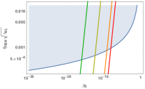
Figure 12: Upper bound on $f_{\text{PBH}}\sqrt{\tau_{\text{NL}}}$ as a function of $\beta_{0}$ in the case of PBH production in a RD epoch (blue curve). Four examples of $f_{\text{PBH}}\sqrt{\tau_{\text{NL}}}$ are plotted as functions of $\beta_{0}$ with the same color coding as those in Fig. 6: $M_{\text{PBH}}/M_{\odot}=10^{-12}$ (green; DM), $10^{-5}$ (dark yellow; OGLE), $10^{1.5}$ (orange), and $10^{3.5}$ (red; SMBH).

In the main text, we have just used $C_{2}\gtrsim 20$ and $C_{2}\geq 5$ to place constraints in the RD case and the MD case, respectively. More precisely, $C_{2}$ depends nonlinearly on the production probability $\beta_{0}$, while $f_{\text{PBH}}$ itself depends linearly on $\beta_{0}$. We have already seen in Fig. 7 that the upper bound on $f_{\text{PBH}}\sqrt{\tau_{\text{NL}}}$ has a nontrivial shape as a function of $\beta_{0}$ in the case of PBH production in the MD epoch. The counterpart in the RD epoch is shown in Fig. 12.

Thus, the constraint (55) is a nonlinear constraint on $\beta_{0}$ depending on $\tau_{\text{NL}}$ and the temperature at which the scale corresponding to the PBH mass $M_{\text{PBH}}$ enters the horizon (RD case), or the reheating temperature $T_{\text{R}}$ (MD case). We can obtain upper bounds on $f_{\text{PBH}}$ as a function of $M_{\text{PBH}}$ (RD) or $T_{\text{R}}$ (MD) for fixed $\tau_{\text{NL}}$ and as a function of $\tau_{\text{NL}}$ for fixed $M_{\text{PBH}}$ (RD) or $T_{\text{R}}$ (MD).

In the case of PBH production in a RD epoch, an essentially same upper bound on $f_{\text{PBH}}(M_{\text{PBH}})$ for fixed $f_{\text{NL}}$ (instead of $\tau_{\text{NL}}$) is given in Fig. 2 of Ref. TY15 . For completeness and with updated Planck data, we show a similar upper bound on $f_{\text{PBH}}(M_{\text{PBH}})$ for some choices of $\tau_{\text{NL}}$ in Fig. 14. The fact that the mass dependence is weak is also shown in Fig 14, in which the upper bound is shown as a function of $\tau_{\text{NL}}$ for fixed masses. To obtain these figures, we solved the relation between $C_{2}$ and $\beta_{0}$ using Eqs. (20) and (22).

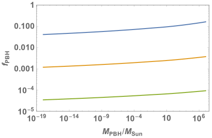
Figure 13: Upper bounds on $f_{\text{PBH}}$ as a function of $M_{\text{PBH}}$ for $\tau_{\text{NL}}=10^{-4}$ (blue line), $10^{-1}$ (orange line), and $10^{2}$ (green line) in the case of PBH production in a RD epoch.

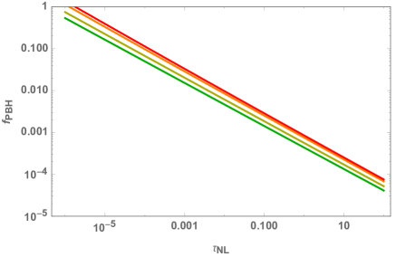
Figure 14: Upper bounds on $f_{\text{PBH}}$ as a function of $\tau_{\text{NL}}$ for $M_{\text{PBH}}/M_{\odot}=10^{-12}$ (green; DM), $10^{-5}$ (dark yellow; OGLE), $10^{1.5}$ (orange; LIGO/Virgo), and $10^{3.5}$ (red; SMBH) in the case of PBH production in a RD epoch.

In the case of PBH production in a MD epoch, the isocurvature constraint on $f_{\text{PBH}}$ is given in terms of $T_{\text{R}}$ instead of $M_{\text{PBH}}$. This is shown in Fig. 16. The constraint as a function of $\tau_{\text{NL}}$ for fixed $T_{\text{R}}$ is shown in Fig. 16. To obtain these figures, the relations between $C_{2}$ and $\beta_{0}$ were numerically solved using results in the main text as shown in Fig. 5.

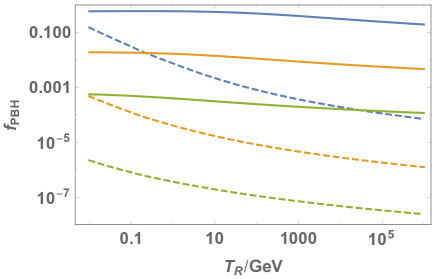
Figure 15: Upper bounds on $f_{\text{PBH}}$ as a function of $T_{\text{R}}$ for $\tau_{\text{NL}}=10^{-4}$ (blue lines), $10^{-1}$ (orange lines), and $10^{2}$ (green lines) in the case of PBH production in a MD epoch. The solid (dashed) lines are based on the second-order (first-order) production mechanism.

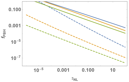
Figure 16: Upper bounds on $f_{\text{PBH}}$ as a function of $\tau_{\text{NL}}$ for $T_{\text{R}}=10^{-2}$ GeV (blue lines), $10^{2}$ GeV (orange lines), and $10^{6}$ GeV (green lines) in the case of PBH production in a MD epoch. The solid (dashed) lines are based on the second-order (first-order) production mechanism.

References

- (1) B. J. Carr, K. Kohri, Y. Sendouda, and J. Yokoyama, Phys. Rev. D81, 104019 (2010).
- (2) S. Bird, I. Cholis, J. B. Muñoz, Y. Ali-Haïmoud, M. Kamionkowski, E. D. Kovetz, A. Raccanelli, and A. G. Riess, Phys. Rev. Lett. 116, 201301 (2016).
- (3) S. Clesse and J. García-Bellido, Phys. Dark Univ. 15, 142 (2017).
- (4) M. Sasaki, T. Suyama, T. Tanaka, and S. Yokoyama, Phys. Rev. Lett. 117, 061101 (2016). Erratum: [Phys. Rev. Lett. 121, no. 5, 059901(E) (2018)]
- (5) M. Sasaki, T. Suyama, T. Tanaka, and S. Yokoyama, Class. Quant. Grav. 35, 063001 (2018).
- (6) B. P. Abbott et al. (LIGO Scientific and Virgo Collaborations), Phys. Rev. Lett. 116, 061102 (2016)
- (7) H. Niikura et al., Nat. Astron. 3, 524 (2019).
- (8) B. Carr, F. Kuhnel, and M. Sandstad, Phys. Rev. D94, 083504 (2016).
- (9) J. García-Bellido, A. Linde, and D. Wands. Phys. Rev. D54, 6040 (1996).
- (10) S. Clesse and J. García-Bellido. Phys. Rev. D92, 023524 (2015).
- (11) H. Niikura, M. Takada, S. Yokoyama, T. Sumi, and S. Masaki, Phys. Rev. D99, 083503 (2019).
- (12) M. Kawasaki, A. Kusenko, and T. T. Yanagida, Phys. Lett. B 711, 1 (2012).
- (13) K. Kohri, T. Nakama, and T. Suyama, Phys. Rev. D90, 083514 (2014).
- (14) M. Kawasaki and K. Murai, Phys. Rev. D100, 103521 (2019).
- (15) B. J. Carr. Astrophys. J. 201, 1 (1975).
- (16) T. Harada, C.-M. Yoo, and K. Kohri, Phys. Rev. D88, 084051 (2013); 89, 029903(E) (2014).
- (17) K. Inomata, M. Kawasaki, K. Mukaida, and T. T. Yanagida, Phys. Rev. D97, 043514 (2018).
- (18) D. H. Lyth, arXiv:1107.1681 [astro-ph.CO]
- (19) K. Kohri, D. H. Lyth, and A. Melchiorri, J. Cosmol. Astropart. Phys. , 04 (2008) 038.
- (20) S. Pi, Y.-l. Zhang, Q.-G. Huang, M. Sasaki, J. Cosmol. Astropart. Phys. , 05 (2018) 042.
- (21) T. J. Gao and Z. K. Guo, Phys. Rev. D98, 063526 (2018).
- (22) P. H. Frampton, M. Kawasaki, F. Takahashi, and T. T. Yanagida, J. Cosmol. Astropart. Phys. 04 (2010) 023.
- (23) J. Martin, T. Papanikolaou, and V. Vennin, arXiv:1907.04236 [astro-ph.CO].
- (24) M. Kawasaki, N. Kitajima, and T. T. Yanagida, Phys. Rev. D87, 063519 (2013).
- (25) K. Kohri, C.-M. Lin, and T. Matsuda, Phys. Rev. D87, 103527 (2013).
- (26) E. Bugaev and P. Klimai, Phys. Rev. D88, 023521 (2013).
- (27) E. Cotner, A. Kusenko, M. Sasaki, and V. Takhistov, J. Cosmol. Astropart. Phys. 10 (2019) 077.
- (28) M. Kawasaki and H. Nakatsuka, Phys. Rev. D 99, 123501 (2019)
- (29) V. De Luca, G. Franciolini, A. Kehagias, M. Peloso, A. Riotto, and C.Ünal, JCAP 07 (2019) 048.
- (30) S. Young, I. Musco, and C. T. Byrnes, J. Cosmol. Astropart. Phys. 11 (2019) 012.
- (31) C. M. Yoo, T. Harada, J. Garriga, and K. Kohri, Prog. Theor. Exp. Phys. 2018, 123E01 (2018).
- (32) V. Atal, J. Garriga, and A. Marcos-Caballero, J. Cosmol. Astropart. Phys. 09 (2019) 073.
- (33) C. M. Yoo, J. O. Gong, and S. Yokoyama, J. Cosmol. Astropart. Phys. 09 (2019) 033.
- (34) J. R. Chisholm, Phys. Rev. D73, 083504 (2006).
- (35) Y. Ali-Haïmoud, Phys. Rev. Lett. 121, 081304 (2018).
- (36) V. Desjacques and A. Riotto, Phys. Rev. D98, 123533 (2018).
- (37) T. Suyama and S. Yokoyama, Prog. Theor. Exp. Phys. 2019, 103E02 (2019).
- (38) Y. Tada and S. Yokoyama, Phys. Rev. D91, 123534 (2015).
- (39) S. Young and C. T. Byrnes, J. Cosmol. Astropart. Phys. 04 (2015) 034.
- (40) M. Raidal, V. Vaskonen, and H. Veermäe, J. Cosmol. Astropart. Phys. 09 (2017) 037.
- (41) G. Ballesteros, P. D. Serpico, and M. Taoso, J. Cosmol. Astropart. Phys. 10 (2018) 043.
- (42) T. Bringmann, P. F. Depta, V. Domcke, and K. Schmidt-Hoberg, Phys. Rev. D 99, 063532 (2019).
- (43) Q. Ding, T. Nakama, J. Silk, and Y. Wang, arXiv:1903.07337 [astro-ph.CO].
- (44) V. Vaskonen and H. Veermäe, arXiv:1908.09752 [astro-ph.CO].
- (45) T. Hasegawa, N. Hiroshima, K. Kohri, R. S. L. Hansen, T. Tram, and S. Hannestad, J. Cosmol. Astropart. Phys. 12 (2019) 012.
- (46) M. Kawasaki, K. Kohri, and N. Sugiyama, Phys. Rev. Lett. 82, 4168 (1999).
- (47) M. Kawasaki, K. Kohri, and N. Sugiyama, Phys. Rev. D 62, 023506 (2000).
- (48) S. Hannestad, Phys. Rev. D 70, 043506 (2004).
- (49) K. Ichikawa, M. Kawasaki, and F. Takahashi, Phys. Rev. D 72, 043522 (2005).
- (50) P. F. de Salas, M. Lattanzi, G. Mangano, G. Miele, S. Pastor, and O. Pisanti, Phys. Rev. D 92, 123534 (2015).
- (51) M. Y. Khlopov and A. G. Polnarev, Phys. Lett. 97B, 383 (1980).
- (52) A. G. Polnarev, and M. Y. Khlopov, Sov. Astron. 26, 9 (1982).
- (53) T. Harada, C.-M. Yoo, K. Kohri, K. Nakao and S. Jhingan, Astrophys. J. 833:61 (2016)
- (54) T. Harada, C. M. Yoo, K. Kohri, and K. I. Nakao, Phys. Rev. D96, 083517 (2017); 99, 069904(E) (2019).
- (55) T. Kokubu, K. Kyutoku, K. Kohri, and T. Harada, Phys. Rev. D98, 123024 (2018).
- (56) Y. B. Zel’dovich, Astron. Astrophys. 5, 84 (1970).
- (57) K. S. Thorne, in Magic Without Magic, ed. J. R. Klauder (Freeman, SanFrancisco, CA, 1972).
- (58) T. Matsubara, Astrophys. J. Suppl. Ser. , 101, 1 (1995).
- (59) T. Matsubara, Phys. Rev. D83, 083518 (2011).
- (60) T. Matsubara, Phys. Rev. D86, 063518 (2012).
- (61) S. Yokoyama and T. Matsubara, Phys. Rev. D87, 023525 (2013).
- (62) T. Matsubara, Phys. Rev. D90, 043537 (2014).
- (63) C. T. Byrnes, M. Sasaki, and D. Wands, Phys. Rev. D74, 123519 (2006).
- (64) L. Boubekeur and D. H. Lyth, Phys. Rev. D73, 021301(R) (2006).
- (65) T. Suyama and M. Yamaguchi, Phys. Rev. D77, 023505 (2008).
- (66) A. R. Liddle and D. H. Lyth, Cosmological Inflation and Large-Scale Structure (Cambridge University Press, Cambridge, England, 2000).
- (67) S. Young, C. T. Byrnes, and M. Sasaki, J. Cosmol. Astropart. Phys. 07 (2014) 045.
- (68) K. M. Smith and M. LoVerde, J. Cosmol. Astropart. Phys. 11 (2011) 009.
- (69) D. Baumann, S. Ferraro, D. Green, and K. M. Smith, J. Cosmol. Astropart. Phys. 05 (2013) 001.
- (70) A. G. Doroshkevich, Astrophysica 6, 30 (1970).
- (71) T. Matsubara and V. Desjacques, Phys. Rev. D93, 123522 (2016).
- (72) N. Afshordi, P. McDonald, and D. N. Spergel, Astrophys. J. 594, L71 (2003).
- (73) J. O. Gong and N. Kitajima, J. Cosmol. Astropart. Phys. 08 (2017) 017.
- (74) Y. Akrami et al. (Planck Collaboration), Astrophys. Space Sci. 364, 69 (2019).
- (75) N. Bartolo, V. De Luca, G. Franciolini, M. Peloso, D. Racco, and A. Riotto, Phys. Rev. D 99, 103521 (2019).
- (76) Y. Tada and S. Yokoyama, Phys. Rev. D 100, 023537 (2019).
- (77) C. Fu, P. Wu, and H. Yu, Phys. Rev. D100, 063532 (2019).
- (78) K. Inomata, M. Kawasaki, K. Mukaida, Y. Tada, and T. T. Yanagida, Phys. Rev. D 95, 123510 (2017).
- (79) K. Kohri and T. Terada, Classical Quantum Gravity 35, 235017 (2018).
- (80) K. Saikawa and S. Shirai, J. Cosmol. Astropart. Phys. 05 (2018) 035.
- (81) B. Carr, T. Tenkanen, and V. Vaskonen, Phys. Rev. D 96, 063507 (2017).
- (82) D. Pogosyan, C. Gay, and C. Pichon, Phys. Rev. D80, 081301(R) (2009); Phys. Rev. D81, 129901(E) (2010).
- (83) C. Gay, C. Pichon, and D. Pogosyan, Phys. Rev. D85, 023011 (2012).