A stellar census in globular clusters with MUSE: Binaries in NGC 3201

We utilize multi-epoch MUSE spectroscopy to study binary stars in the core of the Galactic globular cluster NGC 3201. Our sample consists of $3553$ stars with $54\,883$ spectra in total comprising $3200$ main-sequence stars up to 4 magnitudes below the turn-off. Each star in our sample has between 3 and 63 (with a median of 14) reliable radial velocity measurements within five years of observations. We introduce a statistical method to determine the probability of a star showing radial velocity variations based on the whole inhomogeneous radial velocity sample. Using HST photometry and an advanced dynamical MOCCA simulation of this specific cluster we overcome observational biases that previous spectroscopic studies had to deal with. This allows us to infer a binary frequency in the MUSE FoV and enables us to deduce the underlying true binary frequency of $6.75\pm 0.72\text{\,}\mathrm{\char 37\relax}$ in NGC 3201. The comparison of the MUSE observations with the MOCCA simulation suggests a significant fraction of primordial binaries. We can also confirm a radial increase of the binary fraction towards the cluster centre due to mass segregation. We discovered that in the core of NGC 3201 at least $57.5\pm 7.9\text{\,}\mathrm{\char 37\relax}$ of blue straggler stars are in a binary system. For the first time in a study of globular clusters, we were able to fit Keplerian orbits to a significant sample of 95 binaries. We present the binary system properties of eleven blue straggler stars and the connection to SX Phoenicis-type stars. We show evidence that two blue straggler formation scenarios, the mass transfer in binary (or triple) star systems and the coalescence due to binary-binary interactions, are present in our data. We also describe the binary and spectroscopic properties of four sub-subgiant (or red straggler) stars. Furthermore, we discovered two new black hole candidates with minimum masses ($M\sin{i}$) of $7.68\pm 0.50\text{\,}\mathrm{\textrm{M}_{\odot}}$, $4.4\pm 2.8\text{\,}\mathrm{\textrm{M}_{\odot}}$, and refine the minimum mass estimate on the already published black hole to $4.53\pm 0.21\text{\,}\mathrm{\textrm{M}_{\odot}}$. These black holes are consistent with an extensive black hole subsystem hosted by NGC 3201.

1 Introduction

Multi-star systems are not only responsible for an abundance of extraordinary objects like cataclysmic variables, millisecond pulsars, and low-mass X-ray binaries, but can also be regarded as a source of energy: Embedded in the environment of other stars, like in star clusters, the gravitational energy stored in a multi-star system can be transferred to other stars. In globular clusters with stellar encounters on short time-scales this energy deposit is for example delaying the core collapse (Goodman & Hut, 1989). From a thermodynamic point of view, multi-star systems in globular clusters act as a heat source. The prerequisite for this mechanism is, of course, that globular clusters do contain multi-star systems at some point during their lifetime. For the main-sequence field stars $>$50\text{\,}\mathrm{\char 37\relax}$$ (Duquennoy & Mayor, 1991; Duchêne & Kraus, 2013) in our Milky Way are in multi-star systems. In globular clusters, binary fractions are typically lower than in the field (Milone et al., 2012), but can reach values around $\sim 50\%$ (e.g Sollima et al., 2007; Milone et al., 2012) in central regions. This radial gradient can be explained by mass segregation and indeed is reproduced in simulations (e.g. Fregeau et al., 2009; Hurley et al., 2007). The initial fraction of multi-star systems in globular clusters is changed due to dynamical formation and destruction processes caused by stellar encounters as well as stellar evolution during the (typical long) life time of Galactic globular clusters. The primordial fraction of multi-star systems to single stars for globular clusters therefore cannot be easily inferred from observations (Hut et al., 1992). As a result, the initial fraction is poorly constrained and simulations use values in a wide range from $5\%$ (Hurley et al., 2007) to $100\%$ (Ivanova et al., 2005). Current observations are still consistent with this wide range in primordial binary fractions, depending on which orbit distribution is assumed (Leigh et al., 2015).

Until today there is only one technique with a high discovery efficiency for multi-star systems, namely high precision photometry (Sollima et al., 2007; Milone et al., 2012). It uses the fact that binary stars with both components contributing to the total brightness of one unresolved source have a position in the Colour-Magnitude-Diagram (CMD) differing from single stars. For example, a large number of binaries is located to the brighter (redder) side of the main-sequence (MS). This method is sensitive to binaries on the MS with arbitrary orbital period and inclination. However, no constraints on orbital parameters are possible. The advantage is that this method is efficient in terms of observing time and produces large statistical robust samples. The disadvantage is that in terms of individual binary system properties it only has access to the biased mass-ratio parameter. Milone et al. (2012) investigated 59 Galactic globular clusters with this method using the Hubble Space Telescope (HST). They studied MS binaries with a mass ratio $q>0.5$ and found in nearly all globular clusters a significantly smaller binary frequency than $50\text{\,}\mathrm{\char 37\relax}$. The results show a higher concentration of binaries in the core with a general decreasing binary fraction from the centre to about two core radii by a factor of $\sim 2$. A significant anti-correlation between the cluster binary frequency and its absolute luminosity (mass) was found. Additionally, the authors confirm a significant correlation between the fraction of binaries and the fraction of blue straggler stars (BSS), indicating a relation between the BSS formation mechanism and binaries.

In the literature there are almost no spectroscopic studies of the binarity in globular clusters. One systematic search was done on the globular cluster M4 based on $5973$ spectra of $2469$ stars by Sommariva et al. (2009). They discovered 57 binary star candidates and derived a lower limit of the total binary fraction of $3.0\pm 0.3\text{\,}\mathrm{\char 37\relax}$ for M4.

In light of the important role of binaries in globular clusters, we designed the observing strategy of the MUSE globular cluster survey (Kamann et al., 2018) such that we can infer the binary fraction of every cluster in our sample. For all clusters we aim for at least three epochs of every pointing. For a selection of clusters, namely NGC 104 (47 Tuc), NGC 3201, and NGC 5139 ($\omega$ Cen), we are also able to study individual binary systems in more detail. In this paper we concentrate on the globular cluster NGC 3201. NGC 3201 has, apart NGC 5139, the largest half-light and core radius of all globular clusters in our survey. Its binary fraction within the core radius appears to be relatively high ($12.8\pm 0.8\text{\,}\mathrm{\char 37\relax}$, Milone et al., 2012). In Giesers et al. (2018), we reported a quiescent detached stellar-mass black hole with $4.36\pm 0.41\text{\,}\mathrm{\textrm{M}_{\odot}}$ in this cluster, the first black hole found by a blind spectroscopic survey. Based upon our discovery, NGC 3201 was predicted to harbour a significant population of black holes (see Kremer et al., 2018; Askar et al., 2018a). In our MUSE data, NGC 3201 has the deepest observations, the most epochs to date, and the least crowding. It is therefore the ideal case for our purpose.

This paper is structured as follows. In Sect. 2 we describe peculiar objects which are important in the context of binary star studies in NGC 3201. In Sect. 3 the observations, data reduction and selection of our final sample are discussed. In Sect. 4 we present a MOCCA simulation of the globular cluster NGC 3201 that we used to create a mock observation for comparisons and verifying the following method. We introduce a statistical method to determine the variability of radial velocity measurements and use the method to determine the binary fraction of NGC 3201 in Sect. 5. In Sect. 6 we explain our usage of the tool The Joker to find orbital solutions to individual binary systems and present their orbital parameter distributions. We discuss peculiar objects in our data, like blue straggler stars, sub-subgiants and black hole candidates in Sect. 7. We end with the conclusions and outlook in Sect. 8.

2 Peculiar objects in globular clusters

2.1 Blue straggler stars

In most globular clusters a collection of blue straggler stars can be easily found in the CMD along an extension of the main-sequence beyond the turn-off point. Their positions indicate more massive and younger stars than those of the main-sequence. Without continuing star formation due to lacking gas and dust in globular clusters, mass transfer from a companion is the usual explanation for the formation of a blue straggler. This mass transfer could be on long time-scales, like in compact binary systems, or on short time-scales, as for collisions of two stars (in a binary system or of a priori not associated stars). However, it is still unclear which of these processes contribute to the formation of blue stragglers and how often. Ferraro et al. (1997) discovered a bimodal radial distribution of blue stragglers in M3 and suggested that the blue stragglers in the inner cluster are formed by stellar collisions and those in the outer cluster from merging primordial binaries. Sollima et al. (2008) identified that the strongest correlation in low-density globular clusters is between the number of blue stragglers and the binary frequency of the cluster. They suggested that the primordial binary fraction is one of the most important factors for producing blue stragglers and that the collisional channel to form blue stragglers has a very small efficiency in low-density globular clusters.

Hypki & Giersz (2017) performed numerical simulations of globular clusters with various initial conditions. They found that the number of evolutionary blue stragglers (formed in a compact binary system) is not affected by the density of the globular cluster. In contrast, the number of dynamically created blue stragglers (by collisions between stars) correlates with the density. The efficiencies of both channels strongly depend on the initial semi-major axes distributions. Wider initial orbits lead to more dynamically created blue stragglers. Finally, they found in all globular cluster models at the end of the simulation a constant ratio between the number of blue stragglers in binaries and as single stars $R_{\textrm{B/S}}\sim 0.4$.

A mass distribution of blue stragglers has been estimated by Fiorentino et al. (2014) from pulsation properties of blue stragglers in the globular cluster NGC 6541. They found a mass of $1.06\pm 0.09\text{\,}\mathrm{\textrm{M}_{\odot}}$, which is significantly in excess of the cluster main-sequence turn-off mass ($0.75\text{\,}\mathrm{\textrm{M}_{\odot}}$). Baldwin et al. (2016) found an average mass of blue straggler stars of $1.22\pm 0.12\text{\,}\mathrm{\textrm{M}_{\odot}}$ in 19 globular clusters. Geller & Mathieu (2011) found a surprisingly narrow blue straggler companion mass distribution with a mean of $0.53\text{\,}\mathrm{\textrm{M}_{\odot}}$ in long-period binaries in the open cluster NGC 188. They suggested that this conclusively rules out a collisional origin in this cluster, as the collision hypothesis predicts significantly higher companion masses in their model.

2.2 Sub-subgiant stars

A star in a cluster is called a sub-subgiant (SSG) if its position in the CMD is redder than MS turn-off stars (and its binaries) and fainter than normal subgiant stars. These stars are related to the so called red stragglers (RS) which are redder than normal (red) giant stars. For our study this distinction is not important and we call them hereafter sub-subgiants. The evolution of these stars cannot be explained by single star evolution. Geller et al. (2017a) describe in detail the demographics of SSGs in open and globular clusters and conclude that half of their SSG sample are radial velocity binary stars with typical periods less than $15\text{\,}\mathrm{d}$, $58\text{\,}\mathrm{\char 37\relax}$ are X-ray sources, and $33\text{\,}\mathrm{\char 37\relax}$ are H$\alpha$ emitters. The formation scenarios explained in Leiner et al. (2017) for SSG and RS are isolated binary evolution, the rapid stripping of a subgiant’s envelope, or stellar collisions. So far, from observations and simulations, no channel can be excluded, but it seems that the binary channel is dominant in globular clusters (Geller et al., 2017b).

2.3 SX Phoenicis-type stars

SX Phoenicis-type (SXP) stars are low-luminosity pulsators in the classical instability strip with short periods. In globular clusters they appear as blue straggler stars with an enhanced helium content (Cohen & Sarajedini, 2012). SXP stars show a strong period-luminosity relation, from which distances can be measured. The period range is from $0.02\text{\,}\mathrm{d}$ to $0.4\text{\,}\mathrm{d}$ with typical periods around $\sim$0.04\text{\,}\mathrm{d}$\approx$1\text{\,}\mathrm{h}$$. SXP stars are thought to be formed in binary evolution, but it is not clear whether they are indicative of a particular blue straggler formation channel. The prototype star SX Phoenicis shows a radial velocity amplitude of $19\text{\,}\mathrm{km}\text{\,}{\mathrm{s}}^{-1}$ due to radial pulsation modes (Kim et al., 1993).

2.4 Black holes

Observers are searching for two kinds of black holes in globular clusters. On the one hand, we have no conclusive evidence for central intermediate-mass black holes (IMBH, see Baumgardt, 2017; Tremou et al., 2018). One of the challenges in searching for IMBHs is that typical signatures, such as a central cusp in the surface brightness profile or the velocity dispersion profile can also be explained by a binary star or stellar-mass black hole population (for Omega Cen, see Zocchi et al., 2019). On the other hand, there are known stellar-mass black holes in Galactic globular clusters (e.g. Strader et al., 2012; Giesers et al., 2018). If they are retained, stellar-mass black holes should quickly migrate to the cluster cores due to mass segregation, and strongly affect the evolution of their host globular clusters (e.g. Kremer et al., 2018; Arca Sedda et al., 2018; Askar et al., 2018a, 2019). However, the retention fraction of black holes in globular clusters is largely unknown, which also limits our abilities to interprete gravitational wave detections. For NGC 3201, Askar et al. (2018a) and Kremer et al. (2018) predicted that between 100 and more than 200 stellar-mass black holes should still be present in the cluster, with up to ten in a binary system with a main-sequence star.

3 Observations and data reduction

Table 1: Exposures, observations and integration time per pointing.

Pointing	Exposures	Observations	Total time [min.]
01	49	17	163
02	49	15	143
03	44	15	143
04	36	12	114
Deep	16	4	160
$\sum$	194	63	723

The observational challenge in globular clusters is the crowded field resulting in multiple star blends. For photometric measurements of dense globular clusters, instruments like the ones attached to the HST have just sufficient spatial resolution to get independent measurements of stars down the main-sequence. In the past, spectroscopic measurements of individual globular cluster stars (with a reasonable spectroscopic resolution) were limited by crowding in the cluster centre. Since 2014 we are observing 27 Galactic globular clusters (PI: S. Kamann, formerly S. Dreizler) with the integral field spectrograph Multi Unit Spectroscopic Explorer (MUSE) at the Very Large Telescope (VLT) (Kamann et al., 2018). In the wide field mode, MUSE covers a $1\text{\,}\mathrm{\SIUnitSymbolArcminute}$ x $1\text{\,}\mathrm{\SIUnitSymbolArcminute}$ field of view (FoV) with a spatial sampling of $0.2\text{\,}\arcsec$ and a spectral sampling of $1.25\text{\,}\mathrm{\SIUnitSymbolAngstrom}$ (resolving power of $1770<R<3590$) in the wavelength range from $4750$ to $9350\text{\,}\mathrm{\SIUnitSymbolAngstrom}$. MUSE allows to extract spectra of some thousand stars per exposure.

The overall aim of our stellar census in globular clusters with MUSE is twofold. On the one hand we will investigate the spectroscopic properties of more than half a million of cluster members down to the main-sequence. On the other hand we will investigate the dynamical properties of globular clusters. Upcoming publications are in the field of multiple populations (Husser et al. submitted, Latour et al. submitted, Kamann et al. in preparation), the search for emission line objects (Göttgens et al., 2019, and Göttgens et al., submitted), cluster dynamics like the overall rotation (Kamann et al., 2018), and gas clouds in direction of the clusters (Wendt et al., 2017). Since this survey represents the first blind spectroscopic survey of globular cluster cores, we expect many unforeseen discoveries.

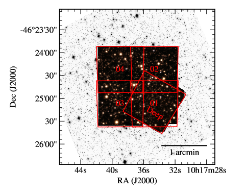
Figure 1: The pointing chart of the MUSE instrument for the globular cluster NGC 3201. The inverted background image is from the ACS globular cluster survey (Sarajedini et al., 2007). The MUSE FoV is a collapsed RGB image created from the spectral cubes. Note the overlapping areas between the pointings.

For this paper, we used all observations of NGC 3201 obtained before May 2019. The pointing scheme can be seen in Fig. 1. In addition to the pointings listed in Kamann et al. (2018), we also implemented a deep field mainly to go deeper on the main-sequence. Table 1 lists the number of visits and total integration times for the different pointings. Our data include adaptive optics (AO) observations, our standard observing mode since the AO system was commissioned in October 2017. The AO observations are treated in the same way as our previous observations. The only difference is that a wavelength window of every spectrum around the sodium lines ($5805\text{\,}\mathrm{\SIUnitSymbolAngstrom}5965\text{\,}\mathrm{\SIUnitSymbolAngstrom}$) has to be masked due to the AO laser emission. During each visit, the pointing was observed with three different instrument derotator angles (0, 90, 180 degrees) in order to reduce systematic effects of the individual MUSE spectrographs.

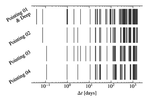
Figure 2: All possible measurement baselines per star and pointing. $\Delta t$ is the time between two observations.

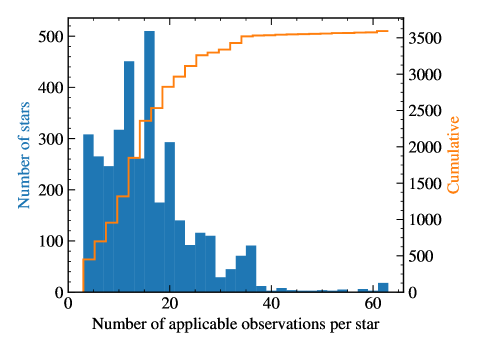
Figure 3: Blue: histogram of applicable (accepted after filtering) number of observations per star. Orange: cumulative distribution of the same data.

Fig. 1 shows our observation scheme for NGC 3201. We secured at least 12 observations per pointing (see Table 1 and Fig. 2). Thanks to the overlapping pointings, up to 63 independent observations per star are available in the central region (see Fig. 3).

To differentiate between radial velocity signals from short period binaries and those of longer period binaries, we observed each of the four pointings twice with a separation of two to three hours in a single night. We already had this distinction sometimes for the stars observed within the same night in the overlapping region of two pointings (like for the published black hole candidate). Without that short baseline a hard binary with a period below one day could mimic the signal of a companion of a black hole candidate at a longer period (temporal aliasing).

The reduction of all exposures was carried out using the standard MUSE pipeline (Weilbacher et al., 2012, 2014). The extraction from the final product of each visit (epoch) is done by a PSF-fitting technique implemented in the software PampelMuse (Kamann et al., 2013). After an extraction is finished the individual spectra are fitted against a synthetic stellar library to determine stellar properties with Spexxy (Husser et al., 2013). The extraction and stellar parameter fitting methods are summarised in Husser et al. (2016) and Kamann et al. (2018).

3.1 Radial velocities

In this study, we want to investigate if a given star is in a binary system using the radial velocity method. Binaries that are able to survive in the dense environment of a globular cluster are so tight, that even HST is not able to spatially resolve the binary components at the distance of NGC 3201. For this reason, the binary system will appear as a single point-like source. Except for the case when both stars have similar brightness (see Sect. 4 on how we handle these binaries), the extracted MUSE spectrum will be dominated by one star. The measured radial velocity variation of this star can be used to determine the properties of the binary system indirectly.

Since we aim for the highest possible radial velocity precision, we checked if the standard wavelength calibration of the MUSE instrument and the uncertainties calculated by the extraction and fitting routines are reliable. For this purpose we analysed the wavelength shift of the telluric lines in the extracted spectra per observation to correct for tiny deviations in the wavelength solution of the pipeline (see Sect. 4.2 in Kamann et al., 2018, for details). We also cross checked the radial velocity of each spectrum obtained by the full-spectrum fit using a cross-correlation of the spectrum with a PHOENIX-library template (Husser et al., 2013) (see criterion in Sect. 3.2). Fig. 4 shows the resulting uncertainties $\epsilon_{v}$ as a function of $S/N$ of the spectra in our final sample of NGC 3201. We get reliable radial velocities from $S/N>5$ spectra (Kamann et al., 2018). At $S/N=10$ the uncertainties are $\epsilon_{v}\approx$7.0\pm 1.7\text{\,}\mathrm{km}\text{\,}{\mathrm{s}}^{-1}$$, at $S/N\gtrsim 50$ the uncertainties are $\epsilon_{v}\approx$1.7\pm 0.5\text{\,}\mathrm{km}\text{\,}{\mathrm{s}}^{-1}$$. These uncertainties represent our spectroscopic radial velocity precision, the accuracy of the MUSE instrument (wavelength shift between two observations) is below $1\text{\,}\mathrm{km}\text{\,}{\mathrm{s}}^{-1}$ (Kamann et al., 2018).

3.2 Selection of the final sample

For the sample selection two things are crucial. Firstly, we only want reliable radial velocities with Gaussian distributed uncertainties. Secondly, our sample should only consist of single and multiple star systems which are cluster members, excluding Galactic field stars. Finally, stars that mimic radial velocity variations due to intrinsic pulsations should be excluded. To ensure this the following filters are applied:

• The reliability of every single spectrum is ensured by the following criteria, which are either 0 (false) and 1 (true).

  We apply a cut for the signal to noise $S/N$ of a spectrum

  $$R_{S/N}=S/N\geq 5\;.{}$$

  The quality of the cross-correlation is checked using the $r$-statistics and $\operatorname{FWHM}$ defined by Tonry & Davis (1979)

  $$R_{\textrm{cc}}=r\geq 4\wedge\operatorname{FWHM}>$10\text{\,}\mathrm{\SIUnitSymbolAngstrom}$\;.{}$$

  A plausible uncertainty $\epsilon_{\textrm{v,cc}}$ of the cross-correlation radial velocity $v_{\textrm{cc}}$

  $$R_{\epsilon_{\textrm{v,cc}}}=\epsilon_{\textrm{v,cc}}>$0.1\text{\,}\mathrm{km}\text{\,}{\mathrm{s}}^{-1}$\;,$$

  and a plausible uncertainty $\epsilon_{\textrm{v}}$ of the full-spectrum fit radial velocity $v$

  $$R_{\epsilon_{\textrm{v}}}=\epsilon_{\textrm{v}}>$0.1\text{\,}\mathrm{km}\text{\,}{\mathrm{s}}^{-1}$$$

  is ensured. We check that the velocity is within $3\sigma$ of the cluster velocity $v_{\textrm{cluster}}$ and the cluster dispersion $\sigma_{\textrm{v,cluster}}$ including the standard deviation taken from the Harris (1996, 2010 edition) catalogue. For typical binary amplitudes we add $30\text{\,}\mathrm{km}\text{\,}{\mathrm{s}}^{-1}$ to the tolerance, yielding

  $$\tiny R_{v}=\frac{|v-v_{\textrm{cluster}}|}{\sqrt{\epsilon_{\textrm{v}}^{2}+\sigma_{\textrm{v,cluster}}^{2}+($30\text{\,}\mathrm{km}\text{\,}{\mathrm{s}}^{-1}$)^{2}}}\leq 3\;.{}$$

  The last criterion is the check if cross-correlation and full-spectrum fit are compatible within $3\sigma$ with each other,

  $$R_{v=v_{\textrm{cc}}}=\frac{|v-v_{\textrm{cc}}|}{\sqrt{\epsilon_{\textrm{v}}^{2}+\epsilon_{\textrm{v,cc}}^{2}}}\leq 3\;.{}$$

  We combine all these criteria in an empirically weighted equation, which gives us a result between 0 and 1,

  $$R_{\textrm{total}}=(2R_{S/N}+10R_{\textrm{cc}}+R_{\epsilon_{\textrm{v,cc}}}+3R_{v}+2R_{\epsilon_{\textrm{v}}}+5R_{v=v_{\textrm{cc}}})/23\;.{}$$

  A radial velocity is considered as reliable if the reliability $R_{\textrm{total}}$ surpasses $80\text{\,}\mathrm{\char 37\relax}$.

• We exclude spectra which are extracted within 5 px from the edge of a MUSE cube to avoid systematic effects.

• We exclude spectra where PampelMuse was unable to deblend multiple nearby HST/ACS sources (this is of course seeing dependent and affects mostly faint sources).

• To identify confusion or extraction problems in a MUSE spectrum, we calculated broad-band magnitudes from the spectrum in the same passband that was used in the extraction process and calculated the differences between input and recovered magnitudes. We accept only spectra with a magnitude accuracy $>$80\text{\,}\mathrm{\char 37\relax}$$ (see Sect. 4.4 in Kamann et al., 2018, for more details).

• In some low S/N cases the cross-correlation and full-spectrum fit returned similar but wrong radial velocities due to noise in the spectrum. These could be outliers by several $100\text{\,}\mathrm{km}\text{\,}{\mathrm{s}}^{-1}$ introducing a strong variation in the signal and passing the reliability criteria described before. To find outliers we generally compare all radial velocities $v_{i}$ (with their uncertainties $\epsilon_{v,i}$) of a single star with each other. We define the set of all radial velocities as $A=\{v_{i}\}$. An outlier $v_{x}$ in the subset $B=A\,\diagdown\,\{v_{x}\}$ of all radial velocities except the inspected radial velocity, is identified with

  $$\frac{\sigma_{A}}{\sigma_{B}}>\kappa\wedge\frac{|v_{x}-\tilde{B}|}{\epsilon_{v,x}+\sigma_{B}}>\kappa\quad\textrm{with}\;\kappa=3\;.$$

  $\tilde{B}$ is the median of the radial velocities $v_{i}$ in the set $B$. $\sigma$ is the standard deviation of the corresponding quantity. Using this equation outliers are identified and excluded from further analyses.

• We manually set the binary probability in our sample to 0 for 10 RR Lyrae- and 5 SX Phoenicis-type stars known in the Catalogue of Variable Stars in Galactic Globular Clusters (Clement et al., 2001; Clement, 2017) and Arellano Ferro et al. (2014).

• Since NGC 3201 has a heliocentric radial velocity of $494.0\pm 0.2\text{\,}\mathrm{km}\text{\,}{\mathrm{s}}^{-1}$ and a central velocity dispersion of $5.0\pm 0.2\text{\,}\mathrm{km}\text{\,}{\mathrm{s}}^{-1}$ (Harris, 1996, 2010 edition), we select members by choosing stars with mean radial velocities $>$400\text{\,}\mathrm{km}\text{\,}{\mathrm{s}}^{-1}$$.

• Our final sample only consists of member stars with at least 3 spectra per star after all filters have been applied.

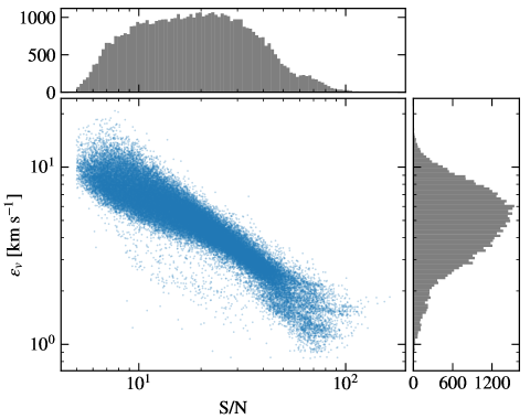
Figure 4: Radial velocity uncertainties $\epsilon_{v}$ of all spectra in the sample used for NGC 3201 as a function of the spectral signal-to-noise.

We end up with $3553$ stars and $54\,883$ spectra out of $4517$ stars and $68\,084$ spectra in total. Due to different observational conditions the stars near the confusion limit cannot be extracted reliably from every observation. Fig. 3 shows a histogram of all applicable observations per star for the final sample of NGC 3201. We have $3285$ ($91\text{\,}\mathrm{\char 37\relax}$) stars with five or more epochs, $2637$ ($73\text{\,}\mathrm{\char 37\relax}$) with ten or more epochs, and $918$ ($26\text{\,}\mathrm{\char 37\relax}$) stars with 20 or more epochs.

3.3 Mass estimation

We estimate the mass of each star photometrically by comparing its colour and magnitude from the ACS globular cluster survey (Sarajedini et al., 2007; Anderson et al., 2008) with a PARSEC isochrone (Bressan et al., 2012). For the globular cluster NGC 3201, we found the best matching isochrone compared to the whole ACS Colour-magnitude diagram (CMD) with the isochrone parameters [M/H] = $-1.39\text{\,}\mathrm{d}\mathrm{e}\mathrm{x}$ (slightly above the comparable literature value $[\mathrm{Fe/H}]$ = $-1.59\text{\,}\mathrm{d}\mathrm{e}\mathrm{x}$, Harris, 1996, 2010 edition), age = $11\text{\,}\mathrm{Gyr}$, extinction $E_{B-V}$ = $0.26$, and distance = $4.8\text{\,}\mathrm{kpc}$. The mass for each star is determined from its nearest neighbour on the isochrone. For blue straggler stars we assume a mass of $1.20\pm 0.05\text{\,}\mathrm{\textrm{M}_{\odot}}$ (Baldwin et al., 2016) instead.

3.4 The electronic catalogue

An outline of the final sample of the radial velocities is listed in Table 3. The columns ACS Id, position (RA, Dec.), and V equivalent magnitude from the ACS catalogue (Sarajedini et al., 2007) are followed by the mean observation date of the combined exposures (BMJD), the barycentric corrected radial velocity $v_{\textrm{r}}$, and its uncertainty $\epsilon_{v}$ from our MUSE observations. The last column contains the probability for variability in radial velocity $P(\chi_{i}^{2},\nu_{i})$, determined as described in Sect. 5. Three versions of the catalogue, one with the full final sample (see Sect. 3.2), one with non-member stars, and one with the RR Lyrae and SX Phoenicis stars are available at the CDS and on the project website https://musegc.uni-goettingen.de/.

4 MOCCA simulation of NGC 3201

We want to compare our observations of binaries in NGC 3201 with models. Our first attempt using a toy model with realistic binary parameter distributions for this specific cluster like period, eccentricity, mass ratio, etc. failed since the creation of binaries from these distributions is unrealistic. Moe & Di Stefano (2017) demonstrated that randomly drawing values of these orbital parameter distributions does not lead to realistic currently observed binary distributions even when the parameter distributions themselves are realistic. Especially not for globular clusters where dynamical interactions between stars play an important role. Thus we have to use more sophisticated simulations of globular clusters including all relevant physics for the cluster dynamics and the binary evolution. Simulating the dynamical evolution of realistic globular clusters in a Galactic potential up to a Hubble time is computationally expensive.

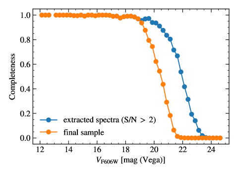
Figure 5: The completeness as a function of magnitude for all MUSE observations of NGC 3201, using photometry from the ACS globular cluster survey (Sarajedini et al., 2007). The fraction of all possible extracted spectra to observed spectra within the MUSE FoV is shown. Blue: extracted spectra with S/N ¿ 2. Orange: extracted spectra in the final sample (see Sect. 3.2). (The uncertainties are smaller than the points.)

Table 2: Globular cluster properties for the MOCCA model in comparison to observed values.

RA	10h17m36$\aas@@fstack{s}$82 (a)
Dec.	-46°24′44$\aas@@fstack{\prime\prime}$9 (a)
Distance to Sun $\mathrm{kpc}$	$4.9\text{\,}\mathrm{kpc}$ (a)
Metallicity [Fe/H]	$-1.59\text{\,}\mathrm{d}\mathrm{e}\mathrm{x}$
Barycentric radial velocity	$494.0\pm 0.2\text{\,}\mathrm{km}\text{\,}{\mathrm{s}}^{-1}$ (a)
	MOCCA	Literature
Central velocity dispersion [$\mathrm{km}\text{\,}{\mathrm{s}}^{-1}$]	$5.23$ (*)	$5.0\pm 0.2$ (a)
Core radius [$\mathrm{pc}$]	$1.54$	$1.85$ (a)
Half-light radius [$\mathrm{pc}$]	$4.16$	$4.42$ (a)
Total V-band luminosity [$L_{\odot}$]	$9.27\text{\times}{10}^{4}$	$8.17\text{\times}{10}^{4}$ (a)
Central surface brightness [$\mathrm{L}_{\odot}\mathrm{/}\mathrm{pc}\mathrm{{}^{2}}$]	$2.25\text{\times}{10}^{3}$	$9.14\text{\times}{10}^{2}$ (a)
Age [Gyr]	$12$	$12.0\pm 0.8$ (b)
Mass [$\mathrm{\textrm{M}_{\odot}}$]	$2.3\text{\times}{10}^{5}$	$(1.49\pm 0.09)\text{\times}{10}^{5}$ (c)
Total binary fraction [$\mathrm{\char 37\relax}$]	$8.72$	—

4.1 The model

An approach that has been used to extensively simulate realistic globular cluster models is the Monte Carlo method for stellar dynamics that was first developed by Hénon (1971). This method combines the statistical treatment of relaxation with the particle based approach of direct N-body methods to simulate the long term evolution of spherically symmetric star clusters. The particle approach of this method enables the implementation of additional physical processes (including stellar/binary evolution) and is much faster than direct N-body methods. In recent years, an extensive number of globular cluster models have been simulated with the MOCCA (MOnte Carlo Cluster simulAtor) (Giersz, 1998; Hypki & Giersz, 2013; Giersz et al., 2013; Askar et al., 2017; Hong et al., 2018; Belloni et al., 2019) and CMC (Cluster Monte Carlo) codes (Joshi et al., 2000; Pattabiraman et al., 2013; Morscher et al., 2015; Rodriguez et al., 2016; Chatterjee et al., 2017).

For the purpose of this project we needed a simulated globular cluster model that would have present-day observational properties comparable to NGC 3201 and that would also contain stellar-mass black holes like the one we found (Giesers et al., 2018). Therefore, we used results from the MOCCA Survey Database I (Askar et al., 2017) to identify initial conditions for a model that had global properties close to NGC 3201 at an age of 12 Gyr. This model has been subsequently refined with additional MOCCA simulations based on slightly modified initial conditions to find an even better agreement with the properties of NGC 3201 at an age of 12 Gyr including total luminosity, core and half-light radii, central surface brightness, velocity dispersion and binary fraction.

The MOCCA code utilizes the Monte Carlo method to compute relaxation. Additionally, it uses the fewbody code (Fregeau et al., 2004, small number N-body integrator) to compute the outcome of strong interactions involving binary stars. MOCCA also makes use of the SSE (Hurley et al., 2000) and BSE (Hurley et al., 2002) codes to carry out stellar and binary evolution of all stars in the cluster. MOCCA results have been extensively compared with results from direct N-body simulations and they show good agreement for both the evolution of global properties and number of specific objects (Giersz et al., 2013; Wang et al., 2016).

The following initial parameters were used for the MOCCA model we simulated specifically for this work to have a comparison to NGC 3201: The initial number of objects was set to $N=5.5\times 10^{5}$. The initial binary fraction was set to $50\text{\,}\mathrm{\char 37\relax}$, resulting in $2.25\text{\times}{10}^{5}$ single stars and $5.5\text{\times}{10}^{5}$ stars in binary systems, thus in total $8.25\text{\times}{10}^{5}$ stars in the initial model. The initial binary properties were set as described in Belloni et al. (2017). The metallicity of the model was set to ($Z=5.1\times 10^{-4}$) to correspond to the observed metallicity of NGC 3201 provided in the Harris (1996, 2010 edition) catalogue. We used a King (1966) model with a central concentration parameter ($W_{0}$) of 6.5. The model had an initial half-mass radius of $1.65\text{\,}\mathrm{pc}$ and a tidal radius of $165\text{\,}\mathrm{pc}$. The initial stellar masses were sampled using a two-component Kroupa (2001) IMF (initial mass function) with masses in the range $0.08M_{\odot}$ to $100M_{\odot}$. Neutron star natal kicks were drawn from the Hobbs et al. (2005) distribution. For black holes, natal kicks were modified according to black hole masses that were computed following Belczynski et al. (2002). The properties of the evolved simulated model at $12\text{\,}\mathrm{G}\mathrm{y}\mathrm{r}$ are listed in Table 2 and compared to literature values. The MOCCA model for NGC 3201 is able to well reproduce the observational core radius, half-light radius, central velocity dispersion, and the V-band luminosity provided in Harris (1996, 2010 edition). The central surface brightness for the MOCCA model is a factor of 2.5 larger than the observed one which is unfortunately not given with an uncertainty. In contrast, McLaughlin & van der Marel (2005), for example, found about twice the observational central surface brightness listed in Harris (1996, 2010 edition). Given the observational uncertainties and limitations, the agreement between the simulated model and the observed values are reasonable.

4.2 The mock observation

We project the simulation snapshot at $12\text{\,}\mathrm{G}\mathrm{y}\mathrm{r}$ in Cartesian coordinates using the COCOA code (Askar et al., 2018b). We use the distance modulus of NGC 3201 at a distance of $4.9\text{\,}\mathrm{kpc}$ (Harris, 1996, 2010 edition) to get the apparent magnitude of all stars. For binary stars we combine the two components into a single magnitude. We select the stars within the MUSE FoV (of all pointings). Additionally we use our observational completeness function for NGC 3201 (see Fig. 5) to select stars accordingly.

After we identified a set of stars comparable to the MUSE observations, we created mock radial velocities for these stars. To this aim, we let our observational data guide the simulation. For every observed star (in our MUSE sample) we randomly picked a MOCCA star with comparable magnitude. We then used the epochs of the observed star to create new radial velocity measurements. For single stars we simply assumed a radial velocity of $0\text{\,}\mathrm{km}\text{\,}{\mathrm{s}}^{-1}$ for every time step. For binaries we calculated the radial velocity for the brighter component from a Keplerian orbit using the MOCCA properties of the binary system (masses, period, inclination, eccentricity, argument of periastron, and periastron time). However, due to the spectral resolution of MUSE its measured radial velocity amplitude will be influenced by the flux ratio of the two components of the binary system. From Monte Carlo simulations we found that the theoretical expected radial velocities $v_{\mathrm{r,theoretical}}$ are linearly damped with the flux ratio:

$$v_{\mathrm{r,measured}}=v_{\mathrm{r,barycentre}}+\left(1-\frac{f_{2}}{f_{1}}\right)\,v_{\mathrm{r,theoretical}}\;.$$ (1)

With the flux of the brighter component $f_{1}$ and the fainter component $f_{2}$. $v_{\mathrm{r,barycentre}}$ is the radial velocity of the barycentre, which can be neglected if only relative velocities are of interest. In the case of both components having the same flux, the measured radial velocity $v_{\mathrm{r,measured}}$ amplitude will be zero. Thus, for example, twin main-sequence binary stars are hard to find. In the case when the fluxes of the components are very different, the observed radial velocity amplitude corresponds to the amplitude of the brighter component. We apply this damping for every simulated radial velocity. Finally we scatter these radial velocities within the uncertainties taken from the MUSE corresponding measurements.

5 The binary fraction of NGC 3201

Sect. 4 reflects the efforts required to create realistic models for globular clusters. We therefore conceived a model independent approach to derive the binary frequency of a globular cluster as well as the probability of an individual star to be radial velocity variable.

5.1 A new method to detect variable stars

We here introduce a general statistical method which could be applied to any inhomogeneous sample with a varying number of (few) measurements and a large range of uncertainties. Here it is applied to radial velocity measurements: To detect radial velocity variations in a given star with $m$ measurements, we compute the $\chi_{i}^{2}$ for the set of measurements $x_{j}$ with uncertainties $\sigma_{j}$ to determine how compatible they are with the constant weighted mean $\overline{x}$ (null hypothesis) of the measurements:

$$\chi_{i}^{2}=\sum_{j=1}^{m}\frac{1}{\sigma_{j}^{2}}\left(x_{j}-\overline{x}\right)^{2}\textrm{\quad with \quad}\overline{x}=\frac{\sum_{j=1}^{m}\frac{x_{j}}{\sigma_{j}^{2}}}{\sum_{j=1}^{m}\frac{1}{\sigma_{j}^{2}}}\;.$$ (2)

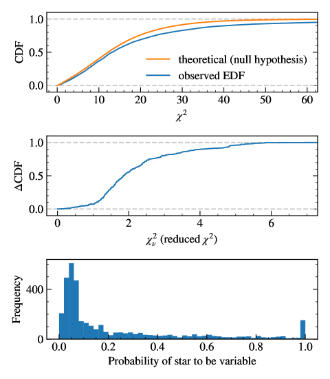
Figure 6: Top panel: superposition of observed empirical distribution function (EDF) and expected theoretical cumulative distribution function (CDF) using the null hypothesis that no variable star exist in sample. Middle panel: resulting $\Delta$CDF. Bottom panel: histogram of variability probabilities in the sample.

A star that shows radial velocity variations larger than the associated uncertainties will have reduced $\chi^{2}>1$ on average. In contrast, a star without significant variations will have reduced $\chi^{2}\approx 1.$ As described in Sect. 3 each star in our sample has its own number of observations and therefore its own number of degrees of freedom ($\nu=m-1$, see Fig. 3). Assuming Gaussian distributed uncertainties for all measurements and a common degree of freedom for all stars, we know the expected $\chi^{2}$-distribution in form of the cumulative distribution function (CDF) $F$ for the null hypothesis that all stars show constant signals. If there are binary stars with radial velocity variations in our sample, there will be an excess of larger $\chi^{2}$ values compared to the null hypothesis. Therefore, the empirical CDF computed from the measured $\chi^{2}$ will increase slower than the CDF computed using the null hypothesis.

For a chosen degree of freedom (e.g. $\nu=3$) we calculate the probability $\bar{P}$ of each star to match the null hypothesis through the comparison of the observed empirical distribution function (EDF) $F_{\textrm{observed}}$ with the expected CDF (comparable to the top panel in Fig. 6):

$$\bar{P}(\chi_{i}^{2},\nu_{i}=3)=\frac{1-F(\chi_{i}^{2},3)_{\textrm{theoretical}}}{1-F(\chi_{i}^{2},3)_{\textrm{observed}}}\;.$$ (3)

Since the EDF $F_{\textrm{observed}}$ is simply the fraction of stars below a given $\chi^{2}$, we divide the number of stars we measured below a given $\chi^{2}$ with the expected number from the known CDF to calculate $P$ (comparable to the middle panel in Fig. 6). The probability of a star to be variable for a given degree of freedom $\nu$ is $P=1-\bar{P}$, i.e.

$$P(\chi_{i}^{2},\nu_{i})=\frac{F(\chi_{i}^{2},\nu_{i})_{\textrm{theoretical}}-F(\chi_{i}^{2},\nu_{i})_{\textrm{observed}}}{1-F(\chi_{i}^{2},\nu_{i})_{\textrm{observed}}}\;.$$ (4)

To use the statistical power of the whole sample with the total number of stars $n$, this equation can be generalised to multiple degrees of freedom by noticing that $n\,F_{\textrm{theoretical}}$ is the expected number of stars below a given $\chi^{2}$. The (expected or observed) total number of stars below a given $\chi^{2}$, taking into account all available degrees of freedom, can be expressed using the number of the stars per degree of freedom $n_{\nu}$ and adding up the contributions from all degrees of freedom in a ’super CDF’:

$$\widehat{S}(\chi_{i}^{2})=\frac{1}{n}\sum_{\nu}{F(\chi_{i}^{2},\nu)\,n_{\nu}}\;,$$ (5)

from which $n\,\widehat{S}$ is the analogue of $n\,F_{\textrm{theoretical}}$ (and $n\,F_{\textrm{observed}}$) for multiple degrees of freedom. Inserting this into Eq. 4 yields

$$P(\chi_{i}^{2},\nu_{i})=\frac{n\,\widehat{S}(\chi_{k}^{2})-k}{n-k}\quad\textrm{with}\;k=\left|\left\{\chi^{2}|\chi^{2}/\nu<\chi_{i}^{2}/\nu_{i}\right\}\right|$$ (6)

where $k$ is the number of stars with a reduced $\chi^{2}$ lower than the one of the given star, i. e. $\chi_{i}^{2}/\nu_{i}$ and $\chi_{k}^{2}$ .

The upper panel of Fig. 6 shows the observed EDF and the theoretical ’super CDF’ $\widehat{S}$. Both functions deviate for increasing $\chi^{2}$, which indicates that stars in the sample not only show statistical variations. The middle panel shows the resulting $\Delta$CDF (Eq. 6) for our sample. If we evaluate it with the reduced $\chi^{2}_{\nu}$ we get the probability for every star to vary in radial velocity. The bottom panel of Fig. 6 shows the resulting binary probability distribution of all NGC 3201 stars in our sample.

Comparing the number of stars with $P>0.5$ to the total number of stars yields the discovery binary fraction. We checked this approach using Monte Carlo simulations for different star samples of single and binary stars. It should be noted that at this $50\text{\,}\mathrm{\char 37\relax}$ threshold there is a balance of false-positives and false-negatives, but that ensures a robust measurement for the overall statistics. Of course, for individual stars the acceptance probability to be a binary should be higher.

The statistical uncertainty of the binary fraction is calculated by the quadratic propagation of the uncertainty determined by bootstrapping (random sampling with replacement) the sample and the difference of the fraction for $P>0.45$ and $P>0.55$ divided by 2 as a proxy for the discriminability uncertainty between binary and single stars.

5.2 Verification of the method on the MOCCA mock observation

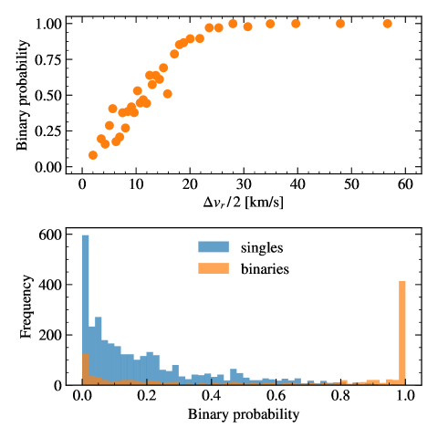
Figure 7: Top panel: the variability probability as a result of the statistical method for all known binaries in the MOCCA mock observation as a function of $\Delta v_{r}\,/\,2$, a proxy for the projected radial velocity semi-amplitude. Bottom panel: histograms of the variability probability for known single and binary stars in the MOCCA mock observation.

To verify the validity of this statistical method, we applied it to the MOCCA mock observation introduced in Sect. 4. For each star we calculated the variability probability according to Eq. 6. We also calculated a kind of semi-amplitude by bisection of the peak to peak of the simulated radial velocities ($\Delta v_{r}\,/\,2$) of each star. In the top panel of Fig. 7 the mean binary probability in relation to this semi-amplitude for all known binaries in the mock observation is presented, using a binning of 30 stars per data point. In view of the radial velocity uncertainties (see Fig. 4) the statistical method gives plausible results: for example $50\text{\,}\mathrm{\char 37\relax}$ of all stars with a semi-amplitude around $10\text{\,}\mathrm{km}\text{\,}{\mathrm{s}}^{-1}$ are recovered. The bottom panel of Fig. 7 shows histograms of the binary probability of the known single stars (in blue) and the known binary stars (in orange). We get a separation of the binary stars (peak at probability $\approx 1$) and single stars (peak at probability $\approx 0$). It shows the power of our approach, as it results in a binary distribution peaked at high probabilities and a single star distribution peaked at low probabilities. Using a threshold of P=0.5 (0.8) would result in a false-positive rate of 324/781 (44/617) stars. These rates are in agreement with the expectations, since the method gives us a balance of false-positives and false-negatives at the $50\text{\,}\mathrm{\char 37\relax}$ threshold, as mentioned before.

The statistical method yields a discovery fraction of $22.1\pm 1.8\text{\,}\mathrm{\char 37\relax}$ for this mock observation. Compared with the true binary fraction in this mock observation of $25.9\text{\,}\mathrm{\char 37\relax}$ we get a discovery efficiency of $85.2\text{\,}\mathrm{\char 37\relax}$. This implies that we can expect to detect the vast majority of binary stars present in our observed MUSE sample.

5.3 Application to the MUSE observations

Using the statistical approach we obtained an observational binary frequency (discovery fraction) of $17.1\pm 1.9\text{\,}\mathrm{\char 37\relax}$ within our MUSE FoV. The bottom panel of Fig. 6 shows the resulting binary probability of our stars in the sample. To determine the true binary frequency of the globular cluster NGC 3201 we have to overcome our observational biases. Our survey is a blind survey and we do not select our targets as in previous spectroscopic studies. Nevertheless, we still have a magnitude limit below which we cannot derive reliable radial velocities and we are confined to the MUSE FoV. In Fig. 5 the magnitude completeness of MUSE stars compared to the ACS globular cluster survey (Sarajedini et al., 2007) of NGC 3201 is shown (blue curve). After filtering (see Sect. 3), we end up with the magnitude completeness of the binary survey (orange curve). To get the binary frequency we have to divide the discovery fraction by the discovery efficiency. As described in Sect. 4, the discovery efficiency cannot be derived by simple assumptions (except for inclination of the binary system). Moreover, the efficiency strongly depends on the number of observations and the sampling per star. Fig. 3 shows that our distribution of applicable observations is inhomogeneous and likewise is our time sampling (see Fig. 2).

We use the MOCCA mock observation to overcome these biases. Assuming the MOCCA simulation is realistic and comparable to our MUSE observation, we found a binary frequency of $20.08\pm 0.22\text{\,}\mathrm{\char 37\relax}$ within our MUSE FoV, taking the discovery efficiency of Sect. 5.2 into account. We can now use the original MOCCA simulation and compare its true binary frequency of $8.72\text{\,}\mathrm{\char 37\relax}$ with the true binary frequency of the mock observation $25.9\text{\,}\mathrm{\char 37\relax}$ and get a factor of $0.336$. Applying this factor and the discovery efficiency it is possible to translate the MUSE discovery fraction into the total binary fraction of NGC 3201 to

$$\large$6.75\pm 0.72\text{\,}\mathrm{\char 37\relax}${}\;.{}$$

The main reason for this value being significantly lower than our observed binary frequency is the central increase of binaries due to mass segregation. Our value is in reasonable agreement with the binary fraction of the MOCCA simulation, $8.72\text{\,}\mathrm{\char 37\relax}$, considering the assumptions that have to be made in Monte Carlo models. This highlights again that the MOCCA simulation that we selected represents an accurate model for NGC 3201.

We also verified to what extent our study is consistent with the results of Milone et al. (2012), who reported a core binary frequency of $12.8\pm 0.8\text{\,}\mathrm{\char 37\relax}$. Without applying any selection function, the MOCCA simulation yields a binary fraction of $12.5\text{\,}\mathrm{\char 37\relax}$ within the core radius of NGC 3201. Hence our results appear to be consistent with the study of Milone et al. (2012) and the apparent differences (with respect to our discovery fraction of $20.08\pm 0.22\text{\,}\mathrm{\char 37\relax}$) can be attributed to selection effects.

5.4 Primordial binaries

We created different MOCCA simulations of NGC 3201 to get a comparable mock observation and thus binary fraction to our observations. The best matching MOCCA simulation (see Sect. 4) has an initial binary fraction of $50\text{\,}\mathrm{\char 37\relax}$ which indicates that a significant fraction of primordial binaries is necessary to reproduce the current observations of NGC 3201.

Recent studies have shown that populations of cataclysmic variables and X-ray sources observed in several globular clusters can be better reproduced with globular cluster simulations that assume high primordial binary fractions (e.g. Rivera Sandoval et al., 2018; Cheng et al., 2018; Belloni et al., 2019). In addition, Leigh et al. (2015) and Cheng et al. (2019) found that a high primordial binary fraction is also necessary to reproduce the binary fraction outside the half-mass radius and the mass segregation we observe in Galactic globular clusters.

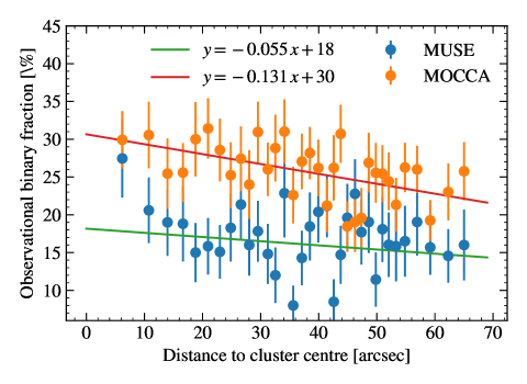
Figure 8: The observational binary fraction of NGC 3201 in radial bins relative to the cluster centre. Blue: MUSE bins with 100 stars per bin. Orange: MOCCA MUSE equivalent mock observation, same bins as MUSE.

5.5 Mass segregation

Due to mass segregation it is expected that binary systems (which are in total more massive than single stars) will migrate towards the centre of a globular cluster (see Sect. 1). Thus the binary fraction should increase towards the cluster centre. In Fig. 8 the observational binary discovery fraction in relation to the projected distance to the centre of the globular cluster is shown. Since we do not have true distances to the cluster centre, any observed radial trend is expected to be somewhat weaker than the underlying trend with true radii. Nevertheless, we found a mild increase of the binary fraction towards the cluster centre. The slope of a simple linear fit is $-0.055\pm 0.003\text{\,}\mathrm{\char 37\relax}$ per arcsec with a Pearson correlation coefficient of $-0.28$. Despite the observational biases and the limited radial distance to the cluster centre this result agrees with the theoretical expectations. Compared to the mock simulation, for which the same projected radial bins have been applied, the result is qualitatively the same. We like to stress that the original MOCCA simulation has a clear radial trend in the binary frequency (using three dimensional radial bins).

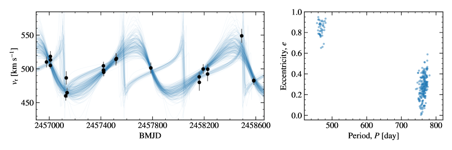
Figure 9: Left: radial velocities (black data points) of the companion of the black hole candidate with ACS Id #5132. The blue curves are the possible orbital solutions determined by The Joker for this star. Right: period-eccentricity plot of these samples.

6 Determination of orbital parameters

Constraining the orbital properties (six standard Keplerian parameters) of a binary system with few or imprecise radial velocity measurements is difficult. Naively one could assume that in dense globular clusters only hard binaries (with high binding energy and typically short period) could survive and should circulise their orbit during their lifetime. However, not only due to dynamical interactions, a significant number of binaries are expected to be on eccentric orbits (Hut et al., 1992). Methods like the generalised Lomb-Scargle periodogram (GLS) (Zechmeister & Kürster, 2009) are good to find periods in unequally sampled data. GLS is good for finding periods in circular orbits, but tends to fail in eccentric configurations. The APOGEE team also faced the same challenges and created a tool named ’The Joker’ (Price-Whelan et al., 2017).

6.1 The Joker

The Joker is a custom Monte Carlo sampler for sparse or noisy radial velocity measurements of two-body systems and can produce posterior samples for orbital parameters even when the likelihood function is poorly behaved.

We follow the method of Price-Whelan et al. (2018) to find orbital solutions for our NGC 3201 stars. Our assumptions to use The Joker are accordingly:

• Two bodies: We assume the multiple star systems in NGC 3201 to consist of two stars or only two stars to be on the dominant timescale for the dynamics of the system (hierarchical multi-star system).

• SB1: The light of the binary components adds up in the MUSE spectrograph as a single source. We assume one of the two binary components does not contribute significantly to the spectrum (single-lined spectroscopic binary = SB1). In the case both components have similar magnitudes (double-lined spectroscopic binary = SB2) it is not possible for us to separate the components for typical radial velocity amplitudes, due to the low spectral resolution of MUSE. As mentioned in Sect. 4, the amplitude of SB2 systems depends on the flux ratio of the two binary components.

• Isolated Keplerian systems: The radial velocity variations are due to orbital motions and not caused by possible intrinsic variations (e.g. pulsations). Moreover, the cluster dynamics happens on a larger timescale than the orbital motion in the binary system.

• Gaussian distributed uncertainties: We ensured all radial velocity uncertainties to be free from systematic effects, independent from each other and represent purely Gaussian noise (for details see Kamann et al., 2018, and Sect. 3.2).

We generated $2^{29}=$536\,870\,912$$ prior samples for the period range $0.3\text{\,}\mathrm{d}$ to $4096\text{\,}\mathrm{d}$. We requested 256 posterior samples for each star with a minimum of 5 observations and a minimum $50\text{\,}\mathrm{\char 37\relax}$ probability to be a variable star. In our sample $515$ met these conditions and could be processed with The Joker. If fewer than 200 posterior samples were found for one star, we used a dedicated MCMC run as described in Price-Whelan et al. (2017) to get 256 new samples. We analysed their posterior distributions and will focus on objects with unimodal or bimodal distributions in the following.

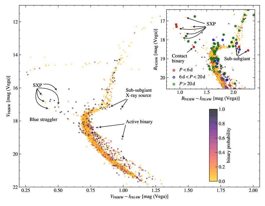
Figure 10: Colour-magnitude diagram of the members of NGC 3201 created with the photometry taken from the HST UV globular cluster survey (Nardiello et al., 2018; Piotto et al., 2015). Colour-coded is the binary probability obtained by our statistical method. Large panel: the full CMD of our sample using V and I equivalent filters is shown. Small panel: a detailed version of the main-sequence turn-off CMD region using B and I equivalent filters is displayed. Additionally, the period $P$ range is indicated by coloured circles where The Joker was able to fit a well constrained Keplerian orbit.

In Fig. 9 the result of this process for one example star (companion of a black hole candidate, more in Sect. 7.3) in our sample is presented. The 256 orbital solutions (in blue) represent the posterior likelihood distribution for this star and are in this case in principle two unique solutions with uncertainties. We define this solutions to be bimodal in orbital period. If in this example, only one solution (one cluster in the right panel of Fig. 9) would be present, we would define it as unimodal. In general, we have unimodal samples when the standard deviation of The Joker periods $P$ in logarithmic scale meets the criterion:

$$\sigma_{\ln{P}}<0.5\;.$$ (7)

To identify bimodal posterior samples we use a similar method as described in Price-Whelan et al. (2018): We use the $k$-means clustering with $k=2$ from the scikit-learn package (Pedregosa et al., 2011) to separate two clusters in the posterior samples in orbital period (like the two clusters in the right panel of Fig. 9). Each of the two clusters have to fulfill Eq. 7. We take the most probable (the one with more samples than the other) as the result for this bimodal posterior samples. Finally, we take the median and the standard deviation as uncertainty of all parameters from these results.

6.2 Binary system properties

The CMD in Fig. 10 is created using the newer HST UV globular cluster survey photometry of NGC 3201 (Nardiello et al., 2018; Piotto et al., 2015) which was matched to the photometry of the HST ACS globular cluster survey (Sarajedini et al., 2007; Anderson et al., 2008) we used as an input catalogue for the extraction of the spectra. The binary probability for each star we determined by our statistical method is colour-coded. As expected, many main-sequence binaries positioned to the red of the main-sequence are found by our method. Red giants brighter than the horizontal branch magnitude could not be found in binary systems in our sample. A good check for the statistical method are the chromospherically active binaries, which deviate in our CMD significantly from the main-sequence (see annotation in CMD) and are very well confirmed by the method. More details about the other stellar types are presented in the following Sect. 7.

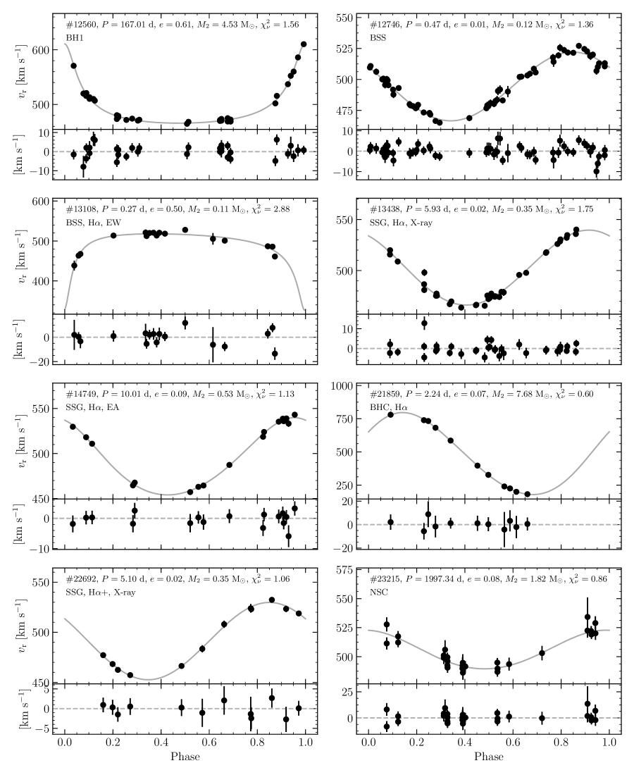
Figure 13: Selection of interesting results from The Joker sorted by ACS Id. The upper panel of every plot shows the radial velocities of the star from our final sample phase folded with the period from the best-fitting model. (Sometimes the uncertainties appear smaller as the data points.) The best-fitting model is plotted with the continues line. The lower panel contains the residuals after subtracting this model from the data. We note the source number, period $P$, eccentricity $e$, invisible mass $M_{2}$ and reduced $\chi^{2}$ of the best fitting model in every plot. See Table 1 for more information to individual stars.

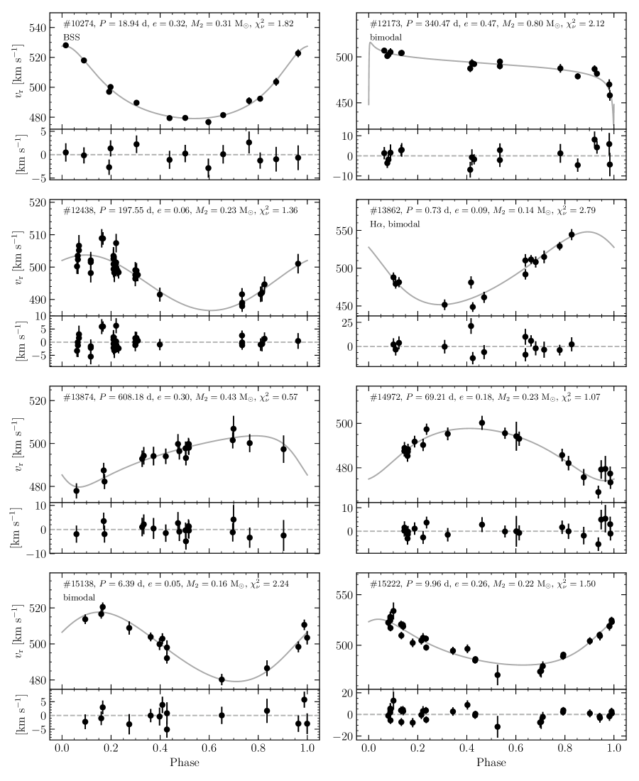
Figure 14: Same as Fig. 13 for a random selection of results from The Joker.

As described in Sect. 6.1 we analysed all stars with a $50\text{\,}\mathrm{\char 37\relax}$ variability probability. We found 95 stars from which 78 stars have unimodal and 17 stars bimodal posterior samples in orbital period. That means the period of these stars is well constrained but does not mean all Keplerian parameters are constrained similarly well. We present the results of The Joker in LABEL:table:binaries with the star position, magnitude, a selection of the fitted parameters (period, eccentricity, amplitude, visible mass), and the derived invisible minimum (companion) mass. The comment column contains additional information to individual stars as explained in the table notes. For a selection of interesting stars of this table we show the best Keplerian fit in Fig. 13 and a blind random set in Fig. 14. These plots show in the upper panel the radial velocities $v_{r}$ of an individual star from our final sample phase folded with the period from the best-fitting model. The lower panel contains the residuals after subtracting this model from the data. In addition to the identifier (ACS Id), position and magnitude from the ACS catalogue (Sarajedini et al., 2007), we note the period $P$, eccentricity $e$, invisible minimum mass $M_{2}$, reduced $\chi^{2}$ of the best fitting model, and the comment in every plot for convenience.

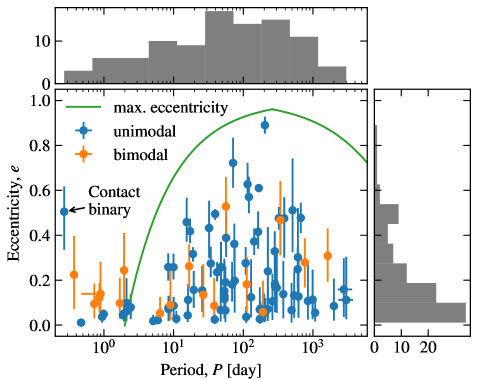
Figure 11: Eccentricity-period plot of the well constrained binaries in NGC 3201. Binaries with unimodal (blue) and bimodal (orange) solutions in the posterior period sampling. The maximum eccentricity in green represents the theoretical limit (above a $2\text{\,}\mathrm{d}$ period) to which binary systems are stable (see Sect. 6.2).

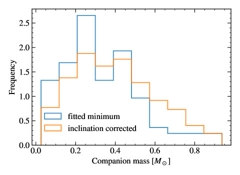
Figure 12: The companion masses (¡ $1\text{\,}\mathrm{\textrm{M}_{\odot}}$) of the well constrained binaries in NGC 3201 are shown. The blue histogram contains the fitted results (minimum masses) from The Joker, whereas the orange histogram contains the same results after applying a statistical correction for orbital inclination to obtain the actual companion mass distribution (see Sect. 6.2).

For the first time Fig. 11 shows the eccentricity-period distribution of binaries in a globular cluster. We found binaries in a period range from $0.27\text{\,}\mathrm{d}3000\text{\,}\mathrm{d}$ with eccentricities from 0 to 0.9. The eccentricity distribution is biased towards low eccentricities, because for these orbits fewer measurements are necessary to get a unique solution. In the figure we also show a maximum eccentricity $e_{\textrm{max}}$ power law derived from a Maxwellian thermal eccentricity distribution

$$e_{\textrm{max}}(P)=1-\left(\frac{P}{2\;\textrm{days}}\right)^{-2/3}\quad\textrm{for}\;P>2\;\textrm{days}$$ (8)

for a given period $P$ (Moe & Di Stefano, 2017). This represents the binary components having Roche lobe fill factors $\leq$70\text{\,}\mathrm{\char 37\relax}$$ at periastron. All binaries with $P<$2\text{\,}\mathrm{d}$$ should have circular orbits due to tidal forces. Additionally, we also take dynamical star interactions into account by using a limit on the orbital velocity at apoastron. The orbital velocity should always be higher than the central cluster dispersion of $5\text{\,}\mathrm{km}\text{\,}{\mathrm{s}}^{-1}$ of NGC 3201 (Harris, 1996, 2010 edition). This limit on eccentricity is dominant for periods $>$260\text{\,}\mathrm{d}$$. Except for the contact binary star (ACS Id: #13108, see LABEL:table:binaries) all stars behave accordingly. Note that when the eccentricity distribution of one star peaked at zero we still took the median like in all other distributions. Therefore the stars below $P<2$ are consistent within their uncertainty with $e=0$. Fig. 11 also clearly shows that not all binaries in globular clusters have been circularised over the lifetime of a globular cluster. We, however, do not find high-eccentric long-period (e.g. $e>0.6$ and $P>$300\text{\,}\mathrm{d}$$) binaries within the eccentricity limit. This could either be due to our observational bias or an effect which restricts the eccentricity even further.

Fig. 12 shows the minimum companion masses of the well constrained binaries (blue histogram). In orange all masses are resampled 1000 times from their fitted mass divided by $\sin{i}$ to obtain the actual companion mass distribution. The inclination $i$ is taken from a sinusoidal detection probability distribution between 0 to $\pi/2$ with a cutoff mass of $0.8\text{\,}\mathrm{\textrm{M}_{\odot}}$ (roughly maximum normal stellar mass in NGC 3201). This results in a linear anti-correlation between the companion mass and the frequency of binaries having this companion mass. As explained in Sect. 4 we have a bias towards binaries with both components having different luminosities. Milone et al. (2012) found a flat mass ratio distribution throughout all clusters above a mass ratio $>0.5$. The pairing fraction of our binaries is beyond the scope of this paper, since we would need to correct for the luminosity ratio effect and the selection function of The Joker, which is currently unknown in our case.

Noteworthy is that all red giant binaries in our sample with well constrained orbits have periods larger than $100\text{\,}\mathrm{d}$. This corresponds to a minimum semi-major axis of $\gtrsim$0.5\text{\,}\mathrm{AU}$$ and is consistent with not having Roche-lobe overflow in the binary system.

7 Peculiar objects in NGC 3201

7.1 Blue straggler stars and SX Phoenicis-type stars

Our sample of NGC 3201 contains 40 blue stragglers with sufficient observations and signal to noise. From these stars, 23 are likely in binary systems while 17 are not (including the SX Phoenicis-type stars assumed to be single stars). This observational binary fraction of $57.5\pm 7.9\text{\,}\mathrm{\char 37\relax}$ is much higher than the one of all cluster stars or even the Milky Way field stars (see Sect. 1). Our ratio of binaries to single blue straggler stars $R_{\textrm{B/S}}=1.35$ in the core of NGC 3201 is significantly higher than the prediction by Hypki & Giersz (2017) of $R_{\textrm{B/S}}\sim 0.4$, but could also be explained by an overabundance of the more massive blue straggler binaries (compared to single blue stragglers) due to mass segregation. Nevertheless, this high binary fraction strongly suggests that most of the blue stragglers in our sample were formed within a binary system. As in Sect. 2 explained, a cluster member needs additional mass to become a blue straggler. Two formation scenarios are consistent with such a high binary fraction: (1) mass transfer within a triple star system (e.g. Antonini et al., 2016), (2) stellar mergers induced by stellar interactions of binary systems with other binaries or single stars (e.g. Leonard, 1989; Fregeau et al., 2004).

From these 23 blue straggler binaries The Joker could find 11 highly constrained solutions, three are extremely hard binaries (¡ $1\text{\,}\mathrm{d}$) with a minimum companion mass ranging from $0.11\text{\,}\mathrm{\textrm{M}_{\odot}}0.24\text{\,}\mathrm{\textrm{M}_{\odot}}$ and six relatively wide (¿ $100\text{\,}\mathrm{d}$) with minimum companion masses ranging from $0.35\text{\,}\mathrm{\textrm{M}_{\odot}}0.67\text{\,}\mathrm{\textrm{M}_{\odot}}$. The remaining 2 blue stragglers are in between the period and companion mass range (see stars in LABEL:table:binaries with comment ’BSS’ for more details). Fig. 10 shows the blue stragglers and their period range in a colour-magnitude diagram. We also identified five blue straggler stars as known SX Phoenicis-type variable stars in the Catalogue of Variable Stars in Galactic Globular Clusters (Clement et al., 2001; Clement, 2017) and one of them as a SX Phoenicis candidate in Arellano Ferro et al. (2014). We also see their pulsations (similar to the RR Lyrae-type stars) as a radial velocity signal up to amplitudes of $18\text{\,}\mathrm{km}\text{\,}{\mathrm{s}}^{-1}$. We cannot distinguish between the pulsation signal and a possible signal induced by a binary companion, thus we consider these stars to be single stars and the velocity variability solely explained by radial pulsations.

Mass transfer in a relatively wide blue straggler binary system is almost impossible. Thus, only the three hard binaries are likely to result from this process. It is obvious that mass transfer is taking place in the contact binary system with ACS Id #13108. On the other hand, head-on collisions of single stars would result in single blue stragglers and are extremely unlikely in a low-density cluster such as NGC 3201. Therefore, it is more likely that a significant fraction of the blue stragglers in our sample result from coalescence in systems with $\geq 3$ stars. The complex behaviour of such systems favours configurations that result in the coalescence of two of its members (e.g. Leonard, 1989; Fregeau et al., 2004; Antonini et al., 2016). If more than two stars in the formation of blue stragglers are involved, this could also mean that hard blue straggler binary systems could have a third outer component inducing an additional, much weaker signal. We could not identify such a signal in our data. For example, the star with ACS Id #12746 (see radial velocity signal in Fig. 13) is the most central hard blue straggler binary in our sample with 63 observations, but its radial velocity curve does not contain any significant additional signal.

The projected spin velocities ($V\sin{i}$) of blue stragglers have been suggested as a possibility to infer their ages and origins (e.g. Leiner et al., 2018). $V\sin{i}$ measurements of blue stragglers in NGC 3201 have been performed by Simunovic & Puzia (2014) and cross-matching their sample with our data results in a subset of five blue stragglers with spin velocities ranging from $34.6\pm 1.6\text{\,}\mathrm{km}\text{\,}{\mathrm{s}}^{-1}$ to $135.2\pm 3.5\text{\,}\mathrm{km}\text{\,}{\mathrm{s}}^{-1}$. We note that all of them are binary systems. However, no clear picture emerges regarding a possible relation between spin velocity and orbital properties.

As introduced, SX Phoenicis-type stars are likely formed in binary evolution. That is why it is possible for them to have a companion, but the companions radial velocity signal would be hidden in the pulsation signal.

7.2 Sub-subgiant stars

We found four sub-subgiant (SSG) stars within our MUSE FoV (see position in Fig. 10). Assuming the radial velocity changes are only Keplerian (and not by pulsations), The Joker could determine unique Keplerian solutions for all of them (see stars in LABEL:table:binaries with comment ’SSG’).

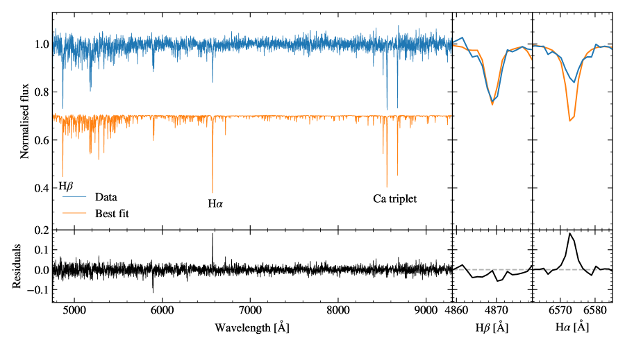
Figure 15: Spectrum of the sub-subgiant with ACS Id #13438. The top panel shows one normalised observed spectrum in blue and the best-fitting PHOENIX spectrum offset by 0.3 in orange. The bottom panel shows the residuals after subtracting the best fit from the data. The right panels show a zoom at the H$\beta$ and H$\alpha$ line with a filled-in observed H$\alpha$ line in contrast to the best fit (not offset).

Fortunately the SSG with ACS Id #14749 (see also plot in Fig. 13) is a known detached eclipsing binary with a period of $10.0037\text{\,}\mathrm{d}$ (Kaluzny et al., 2016) and we found the same period $10.006\pm 0.002\text{\,}\mathrm{d}$ with our method. But this also means the system is observed edge-on and our companion mass is its true mass. The visible star shows a radial velocity amplitude of $42.9\pm 1.5\text{\,}\mathrm{km}\text{\,}{\mathrm{s}}^{-1}$ with a very low eccentricity of $0.09\pm 0.07$, and a companion mass of $0.53\pm 0.04\text{\,}\mathrm{\textrm{M}_{\odot}}$ for an assumed primary mass of $0.82\pm 0.05\text{\,}\mathrm{\textrm{M}_{\odot}}$. That makes a system mass of $1.35\text{\,}\mathrm{\textrm{M}_{\odot}}$ and considering mass transfer, one possible pathway could be towards the blue straggler region (Leiner et al., 2017). Compared to our best fitting model spectrum (and to a well fitted H$\beta$ line) all spectra of this star show a partially filled-in H$\alpha$ absorption line (the absorption is not as deep as expected, see Fig. 15 as an example). This could mean that mass transfer is already underway. In this case this could be used to infer an accretion rate, but is beyond the scope of this paper.

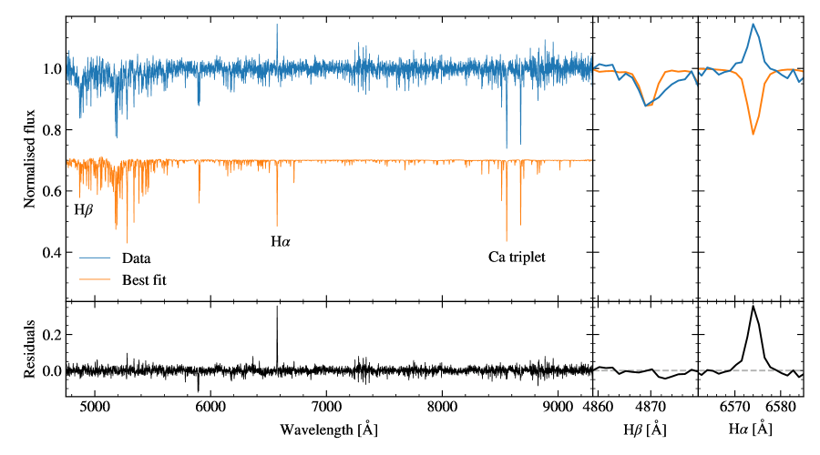
Figure 16: Same as Fig. 15 for the sub-subgiant with ACS Id #22692. Note that in contrast to star #13438 (cf. Fig. 15), this star shows an observed H$\alpha$ emission line.

The two short period ($<$6\text{\,}\mathrm{d}$$, #22692, #13438) sub-subgiants show X-ray emission according to the November 2017 pre-release of the Chandra Source Catalog Release 2.0 (Evans et al., 2010). The SSG (#22692) with the $5.1\text{\,}\mathrm{d}$ period actually has significant varying H$\alpha$ emission lines in most of our spectra. One spectrum of this star with H$\alpha$ in emission is presented in Fig. 16. The maximum emission line is twice as strong as the minimum line compared to the continuum. Again, it would be interesting to calculate the accretion rate for this case, but is beyond the scope of this paper. The SSG (#13438) with the $5.9\text{\,}\mathrm{d}$ period has partially filled-in H$\alpha$ absorption lines in all spectra like the eclipsing SSG described before. One spectrum of this star with the filled-in H$\alpha$ line is shown in Fig. 15. Both short period sub-subgiants have a similar semi-amplitude of $\sim$37\text{\,}\mathrm{km}\text{\,}{\mathrm{s}}^{-1}$$, no eccentricity and a minimum companion mass of $0.35\pm 0.03\text{\,}\mathrm{\textrm{M}_{\odot}}$.

The SSG (#11405) has with $17.2\text{\,}\mathrm{d}$ the longest period, unlike the other stars a relatively high eccentricity of 0.4 and a small minimum companion mass of $0.15\text{\,}\mathrm{\textrm{M}_{\odot}}$.

The detection of a dozen more SSGs and RSs in our MUSE globular cluster sample will be published in the emission line catalogue of Göttgens et al. subm.

7.3 Black hole candidates

Here we report our new measurements for the stellar-mass black hole (BH) candidate in NGC 3201 previously published in Giesers et al. (2018). The additional observations perfectly match the known orbital model and confirm the BH minimum mass to be $4.53\pm 0.21\text{\,}\mathrm{\textrm{M}_{\odot}}$. The deviation to the previously minimum mass of $4.36\pm 0.41\text{\,}\mathrm{\textrm{M}_{\odot}}$ is within the uncertainties. Furthermore, the observations fill in the apoapsis which was missed by previous observations (see #12560 in Fig. 13) and exclude other possible orbital solutions. We would like to emphasise that this star has been analysed with The Joker and MCMC like all other stars, without the effort invested in it as in Giesers et al. (2018).

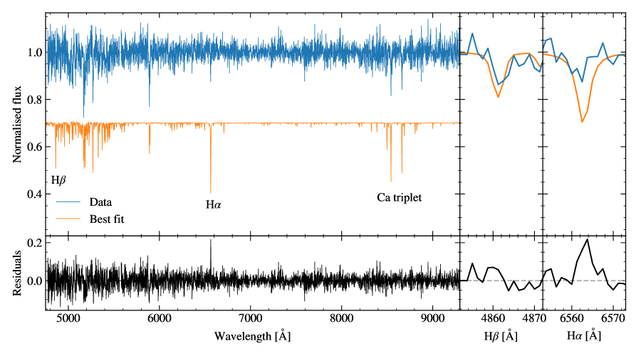
Figure 17: Same as Fig. 15 for the companion of the black hole candidate with ACS Id #21859.

In our full sample of NGC 3201 we detected two additional BH candidates with solutions from the fit of The Joker. LABEL:table:binaries shows the resulting properties of these binary systems with ACS Id #21859 and #5139. Both systems are faint with extracted spectra of S/N $\leq 10$. Remarkable is the system (#21859) with a unique solution and a semi-amplitude of about $300\text{\,}\mathrm{km}\text{\,}{\mathrm{s}}^{-1}$, we cannot explain the radial velocity curve shown in Fig. 13 with other explanations than an unseen companion with a minimum mass of $7.68\pm 0.50\text{\,}\mathrm{\textrm{M}_{\odot}}$. The other system (#5132) has two solutions with the more probable ($82\text{\,}\mathrm{\char 37\relax}$ probability) minimum companion mass of $4.40\pm 2.82\text{\,}\mathrm{\textrm{M}_{\odot}}$ and the less probable of $1.10\pm 0.20\text{\,}\mathrm{\textrm{M}_{\odot}}$. This candidate is not well constrained and needs more observations to be confirmed as a BH. To our knowledge, both sources do not have an X-ray or radio counterpart. This is remarkable in the case of #21859, as the presence of a partially filled-in H$\alpha$ line in the MUSE spectra suggests that accretion is present. We show a combination of all spectra shifted to rest-frame in Fig. 17.

In light of the recent results based on Monte Carlo simulations, it appears feasible that NGC 3201 hosts several BHs in binaries with main-sequence stars. Both Kremer et al. (2018) and Askar et al. (2018a) predict the presence of at least $\sim 100$ BHs in the cluster, with tens of them in binaries with other BHs or bright companions. More specifically, in the best model of Kremer et al. (2018), four BHs have main-sequence-star companions. Interestingly, all of those systems show eccentricities $\gtrsim 0.6$, add odds with the new candidates that we discovered (cf. LABEL:table:binaries). On the other hand, the semi-major axes of our candidates of $0.067\text{\,}\mathrm{AU}$ and $2.804\text{\,}\mathrm{AU}$ are within the range of semi-major-axis values that Kremer et al. (2018) found in their best model of NGC 3201 (see their Fig. 3).

Our MOCCA snapshot at $12\text{\,}\mathrm{G}\mathrm{y}\mathrm{r}$ contains 43 BHs with 33 single BHs, 2 BH-BH binaries, and 6 BH-star binaries. The median mass of all BHs is $16.8\text{\,}\mathrm{\textrm{M}_{\odot}}$ within a range of $3.7\text{\,}\mathrm{\textrm{M}_{\odot}}$ to $78\text{\,}\mathrm{\textrm{M}_{\odot}}$. Two BH-star binaries and 5 single BHs are in the probable mass region of the BH candidates we discussed here. The total number of BHs is lower than the previous predictions, but the number of BHs with detectable companions is consistent with our observations throughout all models.

8 Conclusions and outlook

We elaborated the first binary study from our MUSE survey of 27 Galactic globular clusters on the core of NGC 3201 and showed the variety of results our blind multi-epoch spectroscopic observations reveal. Since modelling a globular cluster contains many imponderables, we developed a statistical method – applicable to any time-variant measurements with inhomogeneous sampling and uncertainties (not only radial velocities) – which can distinguish between a constant and varying signal (like in single and binary stars). We determined an observational binary frequency of $20.08\pm 0.22\text{\,}\mathrm{\char 37\relax}$ using this statistical method. Based on a comparison with an advanced MOCCA simulation of NGC 3201, we calculated a total binary fraction of $6.75\pm 0.72\text{\,}\mathrm{\char 37\relax}$ for all stars in the whole cluster. We confirmed the trend of an increasing binary fraction towards the cluster centre due to mass segregation. We found a significantly higher binary fraction $57.5\pm 7.9\text{\,}\mathrm{\char 37\relax}$ of blue straggler stars compared to the cluster, indicating that the formation of blue stragglers in the core of NGC 3201 is related to binary evolution. For the first time, we presented well constrained Keplerian orbit solutions for a significant amount of stars (95) using the Monte Carlo tool The Joker. Eleven of these are blue straggler stars likely in binary systems and shed light on the properties of these systems. We conclude that both the mass transfer formation scenario and the collisional formation scenario of blue stragglers are present in our data. Collision means in this case the coalescence of two stars during a binary-binary or binary-single encounter. We found four sub-subgiant stars by connecting our MUSE spectroscopy with HST photometry and X-ray observations. Fortunately, we got definite Keplerian solutions for all of them and have insights into their properties for the first time in a globular cluster. Finally, we presented three stellar-mass black hole candidates, from which one is already published (Giesers et al., 2018) and one with a minimum mass of $7.68\pm 0.50\text{\,}\mathrm{\textrm{M}_{\odot}}$ is clearly above a single and even binary neutron star companion mass limit. In total, these black hole candidates in binary systems with main-sequence stars would strongly support the hypothesis that NGC 3201 has an extensive black hole population of up to hundred more black holes (Kremer et al., 2018; Askar et al., 2018a). This cluster, and maybe other globular clusters as well, could be a significant source of gravitational waves.

In a following paper we will present binary fractions in the context of multiple stellar populations within NGC 3201. We will continue to observe $\omega$ Cen and 47 Tuc to have a comparable amount of epochs and will end up with a magnitude more stars per cluster compared to NGC 3201. Finally, we will publish the binary fractions of all clusters in our survey and try to find correlations with cluster parameters.

Appendix A Additional tables and figures

Table 3: Radial velocity measurements: 10 randomly selected rows from the electronically published catalogue with $\sim$50\,000$$ rows.

ACS Id	RA	Dec.	Mag.	BMJD	$v_{\textrm{r}}$	$\epsilon_{v}$	$P(\chi_{i}^{2},\nu_{i})$
	$\mathrm{\SIUnitSymbolDegree}$	$\mathrm{\SIUnitSymbolDegree}$	F606W	$\mathrm{d}$	$\mathrm{km}\text{\,}{\mathrm{s}}^{-1}$	$\mathrm{km}\text{\,}{\mathrm{s}}^{-1}$	%
11317	154.41447	-46.41358	15.77	2457136.4895	491.7	1.5	100
24879	154.38805	-46.40288	19.86	2457009.7918	499.4	6.4	36
10605	154.42077	-46.42044	18.52	2458490.7212	481.6	3.3	17
12088	154.40818	-46.42113	19.09	2457009.8027	491.0	4.7	4
15271	154.38357	-46.41156	20.50	2457786.8727	496.3	7.2	16
23145	154.40307	-46.39943	20.74	2457008.8456	490.3	7.2	60
11426	154.41367	-46.41481	18.17	2458227.6446	506.6	8.0	35
22284	154.41001	-46.39965	20.39	2458227.6446	517.2	8.3	13
22723	154.40600	-46.40560	18.70	2458490.7325	478.0	4.8	7
13914	154.39437	-46.41315	21.16	2458249.5006	495.6	8.1	7

Selection of Joker results

Random selection of Joker results