Forecaster: A Graph Transformer for Forecasting
Spatial and Time-Dependent Data

Abstract

Spatial and time-dependent data is of interest in many applications. This task is difficult due to its complex spatial dependency, long-range temporal dependency, data non-stationarity, and data heterogeneity. To address these challenges, we propose Forecaster, a graph Transformer architecture. Specifically, we start by learning the structure of the graph that parsimoniously represents the spatial dependency between the data at different locations. Based on the topology of the graph, we sparsify the Transformer to account for the strength of spatial dependency, long-range temporal dependency, data non-stationarity, and data heterogeneity. We evaluate Forecaster in the problem of forecasting taxi ride-hailing demand and show that our proposed architecture significantly outperforms the state-of-the-art baselines.

1 Introduction

Spatial and time-dependent data describe the evolution of signals (i.e., the values of attributes) at multiple spatial locations across time [39, 14]. It occurs in many domains, including economics [8], global trade [10], environment studies [15], public health [20], or traffic networks [16] to name a few. For example, the gross domestic product (GDP) of different countries in the past century, the daily temperature measurements of different cities for the last decade, and the hourly taxi ride-hailing demand at various urban locations in the recent year are all spatial and time-dependent data. Forecasting such data allows to proactively allocate resources and take actions to improve the efficiency of society and the quality of life.

However, forecasting spatial and time-dependent data is challenging — they exhibit complex spatial dependency, long-range temporal dependency, heterogeneity, and non-stationarity. Take the spatial and time-dependent data in a traffic network as an example. The data at a location (e.g., taxi ride-hailing demand) may correlate more with the data at a geometrically remote location than a nearby location [16], exhibiting complex spatial dependency. Also, the data at a time instant may be similar to the data at a recent time instant, say an hour ago, but may also highly correlate with the data a day ago or even a week ago, showing strong long-range temporal dependency. Additionally, the spatial and time-dependent data may be influenced by many other relevant factors (e.g., weather influences taxi demand). These factors are relevant information, shall be taken into account. In other words, in this paper, we propose to perform forecasting with heterogeneous sources of data at different spatial and time scales and including auxiliary information of a different nature or modality. Further, the data may be non-stationary due to unexpected incidents or traffic accidents [16]. This non-stationarity makes the conventional time series forecasting methods such as auto-regressive integrated moving average (ARIMA) and vector autoregression (VAR), which usually rely on stationarity, inappropriate for accurate forecasting with spatial and time-dependent data [16, 40].

Recently, deep learning models have been proposed for forecasting for spatial and time-dependent data [16, 35, 11, 36, 7, 38, 34, 40]. To deal with spatial dependency, most of these models either use pre-defined distance/similarity metrics or other prior knowledge like adjacency matrices of traffic networks to determine dependency among locations. Then, they often use a (standard or graph) convolutional neural network (CNN) to better characterize the spatial dependency between these locations. These ad-hoc methods may lead to errors in some cases. For example, the locations that are considered as being dependent (independent) may actually be independent (dependent) in practice. As a result, these models may encode the data at a location by considering the data at independent locations and neglecting the data at dependent locations, leading to inaccurate encoding. Regarding temporal dependency, most of these models use recurrent neural networks (RNN), CNN, or their variants to capture the data long-range temporal dependency and non-stationarity. But it is well documented that these networks may fail to capture temporal dependency between distant time epochs [9, 29].

To tackle these challenges, we propose Forecaster, a new deep learning architecture for forecasting spatial and time-dependent data. Our architecture consists of two parts. First, we use the theory of Gaussian Markov random fields [24] to learn the structure of the graph that parsimoniously represents the spatial dependency between the locations (we call such graph a dependency graph). Gaussian Markov random fields model spatial and time-dependent data as a multivariant Gaussian distribution over the spatial locations. We then estimate the precision matrix of the distribution [6]. The precision matrix provides the graph structure with each node representing a location and each edge representing the dependency between two locations. This contrasts prior work on forecasting — we learn from the data its spatial dependency. Second, we integrate the dependency graph in the architecture of the Transformer [29] for forecasting spatial and time-dependent data. The Transformer and its extensions [29, 3, 33, 4, 22] have been shown to significantly outperform RNN and CNN in NLP tasks, as they capture relations among data at distant positions, significantly improving the learning of long-range temporal dependency [29]. In our Forecaster, in order to better capture the spatial dependency, we associate each neuron in different layers with a spatial location. Then, we sparsify the Transformer based on the dependency graph: if two locations are not connected in the graph, we prune the connection between their associated neurons. In this way, the state encoding for each location is only impacted by its own state encoding and encodings for other dependent locations. Moreover, pruning the unnecessary connections in the Transformer avoids overfitting.

To evaluate the effectiveness of our proposed architecture, we apply it to the task of forecasting taxi ride-hailing demand in New York City [28]. We pick 996 hot locations in New York City and forecast the hourly taxi ride-hailing demand around each location from January 1st, 2009 to June 30th, 2016. Our architecture accounts for crucial auxiliary information such as weather, day of the week, hour of the day, and holidays. This improves significantly the forecasting task. Evaluation results show that our architecture reduces the root mean square error (RMSE) and mean absolute percentage error (MAPE) of the Transformer by 8.8210% and 9.6192%, respectively, and also show that our architecture significantly outperforms other state-of-the-art baselines.

In this paper, we present critical innovation:

• Forecaster combines the theory of Gaussian Markov random fields with deep learning. It uses the former to find the dependency graph among locations, and this graph becomes the basis for the deep learner forecast spatial and time-dependent data.

• Forecaster sparsifies the architecture of the Transformer based on the dependency graph, allowing the Transformer to capture better the spatiotemporal dependency within the data.

• We apply Forecaster to forecasting taxi ride-hailing demand and demonstrate the advantage of its proposed architecture over state-of-the-art baselines.

2 Methodology

In this section, we introduce the proposed architecture of Forecaster. We start by formalizing the problem of forecasting spatial and time-dependent data (Section 2.1). Then, we use Gaussian Markov random fields to determine the dependency graph among data at different locations (Section 2.2). Based on this dependency graph, we design a sparse linear layer, which is a fundamental building block of Forecaster (Section 2.3). Finally, we present the entire architecture of Forecaster (Section 2.4).

2.1 Problem Statement

We define spatial and time-dependent data as a series of spatial signals, each collecting the data at all spatial locations at a certain time. For example, hourly taxi demand at a thousand locations in 2019 is a spatial and time-dependent data, while the hourly taxi demand at these locations between 8 a.m. and 9 a.m. of January 1st, 2019 is a spatial signal. The goal of our forecasting task is to predict the future spatial signals given the historical spatial signals and historical/future auxiliary information (e.g., weather history and forecast). We formalize forecasting as learning a function $h\left(\cdot\right)$ that maps $T$ historical spatial signals and $T+T^{\prime}$ historical/future auxiliary information to $T^{\prime}$ future spatial signals, as Equation (1):

$$\left[\begin{array}[]{ccc}\mathbf{{x}}_{t-T+1},&\cdots,&\mathbf{{x}}_{t};\\ \mathbf{{a}}_{t-T+1},&\cdots,&\mathbf{{a}}_{t+T^{\prime}}\end{array}\right]\overset{h\left(\cdot\right)}{\longrightarrow}\left[\begin{array}[]{ccc}\mathbf{{x}}_{t+1},&\cdots,&\mathbf{{x}}_{t+T^{\prime}}\end{array}\right]$$ (1)

where $\mathbf{{x}}_{t}$ is the spatial signal at time $t$, $\mathbf{{x}}_{t}=\left[\begin{array}[]{ccc}x_{t}^{1},&\cdots,&x_{t}^{N}\end{array}\right]^{T}\in\mathbb{{R}}^{N}$, with $x_{t}^{i}$ the data at location $i$ at time $t$; $N$ the number of locations; $\mathbf{{a}}_{t}$ the auxiliary information at time $t$, $\mathbf{{a}}_{t}\in\mathbb{{R}}^{P}$, $P$ the dimension of the auxiliary information; and $\mathbb{R}$ is the set of the reals.

2.2 Gaussian Markov Random Field

We use Gaussian Markov random fields to find the dependency graph of the data over the different spatial locations. Gaussian Markov random fields model the spatial and time-dependent data $\mathbf{\left\{\mathbf{{x}_{t}}\right\}}$ as a multivariant Gaussian distribution over $N$ locations, i.e., the probability density function of the vector given by $\mathbf{{x}_{t}}$ is

$$f\left(\mathbf{{x}_{t}}\right)=\frac{\left|Q\right|}{\left(2\pi\right)^{\nicefrac{\mathrm{N}}{\mathrm{2}}}}\exp\left(-\frac{1}{2}\left(\mathbf{\mathbf{{x}}}_{t}-\mathbf{\bm{{\mu}}}\right)^{T}Q\left(\mathbf{\mathbf{{x}}}_{t}-\bm{{\mu}}\right)\right)$$ (2)

where $\bm{{\mu}}$ and $Q$ are the expected value (mean) and precision matrix (inverse of the covariance matrix) of the distribution.

The precision matrix characterizes the conditional dependency between different locations — whether the data $x_{t}^{i}$ and $x_{t}^{j}$ at the $i^{\mathrm{{th}}}$ and $j^{\mathrm{{th}}}$ locations depend on each other or not given the data at all the other locations $x_{t}^{-ij}$ ($x_{t}^{-ij}=\left\{x_{t}^{k}\>|\>k\neq i,\,j\right\}$). We can measure the conditional dependency between locations $i$ and $j$ through their conditional correlation coefficient $\mathrm{{Corr}}\left(x_{t}^{i},x_{t}^{j}\>|\>x_{t}^{-ij}\right)$:

$$\mathrm{{Corr}}\left(x_{t}^{i},x_{t}^{j}\>|\>x_{t}^{-ij}\right)=-\frac{Q_{ij}}{\sqrt{Q_{ii}Q_{jj}}}$$ (3)

where $Q_{ij}$ is the $i^{\mathrm{{th}}}$, $j^{\mathrm{{th}}}$ entry of $Q$. In practice, we set a threshold on $\mathrm{{Corr}}\left(x_{t}^{i},x_{t}^{j}\>|\>x_{t}^{-ij}\right)$, and treat locations $i$ and $j$ as conditionally dependent if the absolute value of $\mathrm{{Corr}}\left(x_{t}^{i},x_{t}^{j}\>|\>x_{t}^{-ij}\right)$ is above the threshold.

The non-zero entries define the structure of the dependency graph between locations. Figure 1 shows an example of a dependency graph. Locations 1 and 2 and locations 2 and 3 are conditionally dependent, while locations 1 and 3 are conditionally independent. This principle example illustrates the advantage of Gaussian Markov random field over ad-hoc pairwise similarity metrics — the former leads to parsimonious (sparse) graph representations.

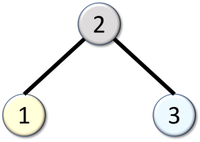
Figure 1: An example of a simple dependency graph.

We estimate the precision matrix by graphical lasso [6], an L1-penalized maximum likelihood estimator:

$$\begin{array}[]{c}\underset{Q}{\textrm{{min}}}\enskip\mathrm{{tr}}\left(SQ\right)-\mathrm{\log}\det\left(Q\right)+\lambda\left\|Q\right\|_{1}\\ s.t.,\enskip Q\in\left\{Q=Q^{T},\;Q\succ 0\right\}\end{array}$$ (4)

where $S$ is the empirical covariance matrix computed from the data:

$$\begin{array}[]{r@{}l}S&{}=\frac{1}{M-1}\sum_{t=1}^{M}\left(\mathbf{\mathbf{{x}}}_{t}-\mathbf{\bm{{\mu}}}\right)^{T}\left(\mathbf{\mathbf{{x}}}_{t}-\bm{{\mu}}\right)\\ \\ \textrm{$\bm{{\mu}}$}&{}=\frac{1}{M}\sum_{t=1}^{M}\mathbf{\mathbf{{x}}}_{t}\end{array}$$ (5)

where $M$ is the number of time samples used to compute $S$.

2.3 Building Block: Sparse Linear Layer

We use the dependency graph to sparsify the architecture of the Transformer. This leads to the Transformer better capturing the spatial dependency within the data. There are multiple linear layers in the Transformer. Our sparsification on the Transformer replaces all these linear layers by the sparse linear layers described in this section.

We use the dependency graph to build a sparse linear layer. Figure 2 shows an example (based on the dependency graph in Figure 1). Suppose that initially the $l^{\mathrm{{th}}}$ layer (of five neurons) is fully connected to the $l+1^{\mathrm{{th}}}$ layer (of nine neurons). We assign neurons to the data at different locations (marked as ”1”, ”2”, and ”3” for locations 1, 2, and 3, respectively) and to the auxiliary information (marked as ”a”) as illustrated next. How to assign neurons is a design choice for users. In this example, assign one neuron to each location and two neurons to the auxiliary information at the $l^{\mathrm{{th}}}$ layer and assign two neurons to each location and three neurons to the auxiliary information at the $l+1^{\mathrm{{th}}}$ layer. After assigning neurons, we prune connections based on the structure of the dependency graph. As locations 1 and 3 are conditionally independent, we prune the connections between them. We also prune the connections between the neurons associated with locations and the auxiliary information to further simplify the architecture. This way, the encoding for the data at a location is only impacted by the encodings of itself and of its dependent locations, better capturing the spatial dependency between locations. Moreover, pruning the unnecessary connections between conditionally independent locations helps avoiding overfitting.

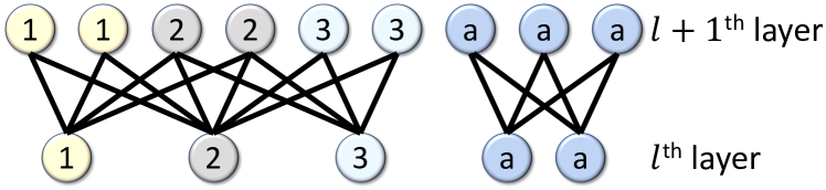
Figure 2: An example of a sparse linear layer based on the dependency graph in Figure 1 (neurons marked as ”1”, ”2”, ”3”, and ”a” are for locations 1, 2, and 3, and auxiliary information, respectively).

Our sparse linear layer is similar to the state-of-the-art graph convolution approaches such as GCN [12] and TAGCN [5, 26] — all of them transform the data based on the adjacency matrix of the graph. The major difference is our sparse linear layer learns the weights for non-zero entries of the adjacency matrix (equivalent to the weights of the sparse linear layer), considering that different locations may have different strengths of dependency between each other.

2.4 Entire Architecture: Graph Transformer

Forecaster adopts an architecture similar to that of the Transformer except for substituting all the linear layers in the Transformer with our sparse linear layer designed based on the dependency graph. Figure 3 shows its architecture. Forecaster employs an encoder-decoder architecture [27], which has been widely adopted in sequence generation tasks such as taxi demand forecasting [16] and pose prediction [30]. The encoder is used to encode the historical spatial signals and historical auxiliary information; the decoder is used to predict the future spatial signals based on the output of the encoder and the future auxiliary information. We omit what Forecaster shares with the Transformer (e.g., positional encoding, multi-head attention) and emphasize only on their differences in this section. Instead, we provide a brief introduction to multi-head attention in the appendix.

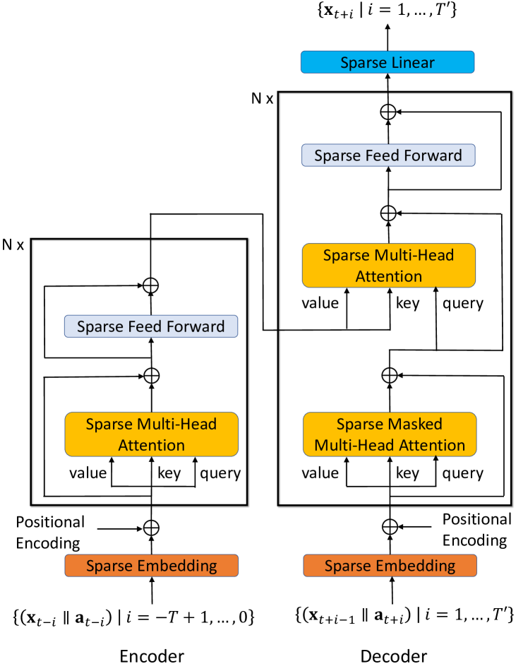
Figure 3: Architecture of Forecaster ($a\parallel b$ represents concatenating vector $a$ with vector $b$).

2.4.1 Encoder

At each time step in the history, we concatenate the spatial signal with its auxiliary information. This way, we obtain a sequence where each element is a vector consisting of the spatial signal and the auxiliary information at a specific time step. The encoder takes this sequence as input. Then, a sparse embedding layer (consisting of a sparse linear layer with ReLU activation) maps each element of this sequence to the state space of the model and outputs a new sequence. In Forecaster, except for the sparse linear layer at the end of the decoder, all the layers have the same output dimension. We term this dimension $d_{model}$ and the space with this dimension as the state space of the model. After that, we add positional encoding to the new sequence, giving temporal order information to each element of the sequence. Next, we let the obtained sequence pass through $N$ stacked encoder layers to generate the encoding of the input sequence. Each encoder layer consists of a sparse multi-head attention layer and a sparse feedforward layer. These layers are the same multi-head attention layer and feedforward layer as in the Transformer, except that sparse linear layers, which reflect the spatial dependency between locations, to replace linear layers within them. The sparse multi-head attention layer enriches the encoding of each element with the information of other elements in the sequence, capturing the long-range temporal dependency between elements. It takes each element as a query, as a key, and also as a value. A query is compared with other keys to obtain the similarities between an element and other elements, and then these similarities are used to weight the values to obtain the new encoding of the element. Note each query, key, and value consists of two parts: the part for encoding the spatial signal and the part for encoding the auxiliary information — both impact the similarity between a query and a key. As a result, in the new encoding of each element, the part for encoding the spatial signal takes into account the auxiliary information. The sparse feedforward layer further refines the encoding of each element.

2.4.2 Decoder

For each time step in the future, we concatenate its auxiliary information with the (predicted) spatial signal one step before. Then, we input this sequence to the decoder. The decoder first uses a sparse embedding layer to map each element of the sequence to the state space of the model, adds the positional encoding, and then passes it through $N$ stacked decoder layers to obtain the new encoding of each element. Finally, the decoder uses a sparse linear layer to project this encoding back and predict the next spatial signal. Similar to the Transformer, the decoder layer contains two sparse multi-head attention layers and a sparse feedforward layer. The first (masked) sparse multi-head attention layer compares the elements in the sequence, obtaining a new encoding for each element. Like the Transformer, we put a mask here such that an element is compared with only earlier elements in the sequence. This is because, in the inference stage, a prediction can be made based on only the earlier predictions and the past history — information about later predictions are not available. Hence, a mask needs to be placed here such that in the training stage we also do the same thing as in the inference stage. The second sparse multi-head attention layer compares each element of the sequence in the decoder with the history sequence in the encoder so that we can learn from the past history. If non-stationarity happens, the comparison will tell the element is different from the historical elements that it is normally similar to, and therefore we should instead learn from other more similar historical elements, handling this non-stationarity. The following sparse feedforward layer further refines the encoding of each element.

3 Evaluation

In this section, we apply Forecaster to the problem of forecasting taxi ride-hailing demand in Manhattan, New York City. We demonstrate that Forecaster outperforms the state-of-the-art baselines (the Transformer [29] and DCRNN [16]) and a conventional time series forecasting method (VAR [19]).

3.1 Evaluation Settings

3.1.1 Dataset

Our evaluation uses the NYC Taxi dataset [28] from 01/01/2009 to 06/30/2016 (7.5 years in total). This dataset records detailed information for each taxi trip in New York City, including its pickup and dropoff locations. Based on this dataset, we select 996 locations with hot taxi ride-hailing demand in Manhattan of New York City, shown in Figure 4. Specifically, we compute the taxi ride-hailing demand at each location by accumulating the taxi ride closest to that location. Note that these selected locations are not uniformly distributed, as different regions of Manhattan has distinct taxi demand. We compute the hourly taxi ride-hailing demand at these selected locations across time. As a result, our dataset contains 65.4 million data points in total (996 locations $\times$ number of hours in 7.5 years). As far as we know, it is the largest (in terms of data points) and longest (in terms of time length) dataset in similar types of study. Our dataset covers various types of scenarios and conditions (e.g., under extreme weather condition). We split the dataset into three parts — training set, validation set, and test set. Training set uses the data in the time interval 01/01/2009 – 12/31/2011 and 07/01/2012 – 06/30/2015; validation set uses the data in 01/01/2012 – 06/30/2012; and the test set uses the data in 07/01/2015 –06/30/2016.

Our evaluation uses hourly weather data from [32] to construct (part of) the auxiliary information. Each record in this weather data contains seven entries — temperature, wind speed, precipitation, visibility, and the Booleans for rain, snow, and fog.

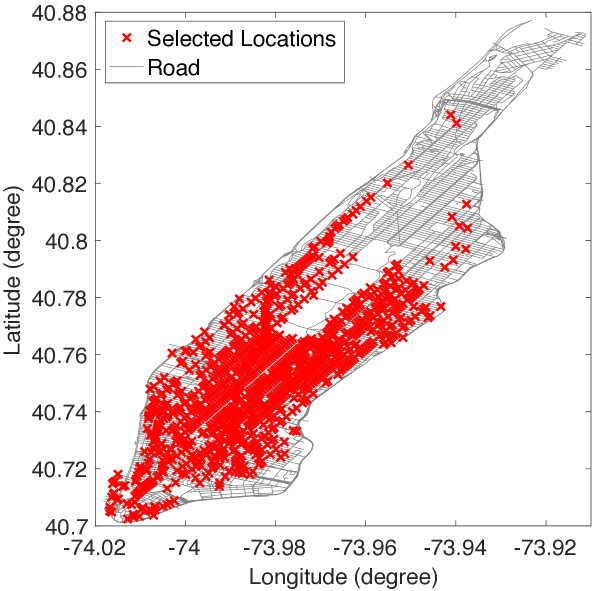
Figure 4: Selected locations in Manhattan.

3.1.2 Details of the Forecasting Task

In our evaluation, we forecast taxi demand for the next three hours based on the previous 674 hours and the corresponding auxiliary information (i.e., use a history of four weeks around; $T=674$, $T^{\prime}=3$ in Equation (1)). Instead of directly inputing this history sequence into the model, we first filter it. This filtering is based on the following observation: a future taxi demand correlates more with the taxi demand at previous recent hours, the similar hours of the past week, and the similar hours on the same weekday in the past several weeks. In other words, we shrink the history sequence and only input the elements relevant to forecasting. Specifically, our filtered history sequence contains the data for the following taxi demand (and the corresponding auxiliary information):

• The recent past hours: $\mathbf{{x}}_{t-i},\;i=0,...,5$ ;

• Similar hours of the past week: $\mathbf{{x}}_{t+i-j\times 24},\;i=-1,...,5,\;j=1,..,6$ ;

• Similar hours on the same weekday of the past several weeks: $\mathbf{{x}}_{t+i-j\times 24\times 7},\;i=-1,...,5,\;j=1,..,4$.

3.1.3 Evaluation Metrics

Similar to prior work [16, 7], we use root mean square error (RMSE) and mean absolute percentage error (MAPE) to evaluate the quality of the forecasting results. Suppose that for the $j^{th}$ forecasting job ($j=1,\cdots,S$), the ground truth is $\left\{x_{t}^{i^{(j)}}\>|\>t=1,\cdots,T^{{}^{\prime}},\>i=1,\cdots,N\right\}$, and the prediction is $\left\{\widehat{x_{t}^{i}}^{(j)}\>|\>t=1,\cdots,T^{{}^{\prime}},\>i=1,\cdots,N\right\}$, where $N$ is the number of locations, and $T^{\prime}$ is the length of the forecasted sequence. Then RMSE and MAPE are:

$$\begin{array}[]{r@{}l}\mathrm{{RMSE}}&{}=\sqrt{\dfrac{1}{ST^{\prime}N}\sum\limits_{j=1}^{S}\sum\limits_{t=1}^{T^{\prime}}\sum\limits_{i=1}^{N}\left(\widehat{x_{t}^{i}}^{(j)}-x_{t}^{i^{(j)}}\right)^{2}}\\ \\ \mathrm{{MAPE}}&{}=\dfrac{1}{ST^{\prime}N}\sum\limits_{j=1}^{S}\sum\limits_{t=1}^{T^{\prime}}\sum\limits_{i=1}^{N}\left|\dfrac{\widehat{x_{t}^{i}}^{(j)}-x_{t}^{i^{(j)}}}{x_{t}^{i^{(j)}}}\right|\end{array}$$ (6)

Following practice in prior work [7], we set a threshold on $x_{t}^{i^{(j)}}$ when computing MAPE: if $x_{t}^{i^{(j)}}<10$, disregard the term associated it. This practice prevents small $x_{t}^{i^{(j)}}$ dominating MAPE.

3.2 Models Details

We evaluate Forecaster and compare it against baseline models including VAR, DCRNN, and the Transformer.

3.2.1 Our model: Forecaster

Forecaster uses weather (7-dimensional vector), weekday (one-hot encoding, 7-dimensional vector), hour (one-hot encoding, 24-dimensional vector), and a Boolean for holidays (1-dimensional vector) as auxiliary information (39-dimensional vector). Concatenated with a spatial signal (996-dimensional vector), each element of the input sequence for Forecaster is a 1035-dimensional vector. Forecaster uses one encoder layer and one decoder layer (i.e., $N=1)$. Except for the sparse linear layer at the end of the decoder, all the layers of Forecaster use four neurons for encoding the data at each location and 64 neurons for encoding the auxiliary information and thus have 4048 neurons in total (i.e., $d_{model}=4\times 996+64=4048$). The sparse linear layer at the end has 996 neurons. Forecaster uses the following loss function:

$${\color[rgb]{0,0,0}\textrm{{loss}}\left(\cdot\right)=\eta\times\textrm{{RMSE}}^{2}+\textrm{{MAPE}}}$$ (7)

where $\eta$ is a constant balancing the impact of RMSE with MAPE, $\eta=8\times 10^{-3}$.

3.2.2 Baseline model: Vector Autoregression

Vector autoregression (VAR) [19] is a conventional multivariant time series forecasting method. It predicts the future endogenous variables (i.e., the spatial signal $\mathbf{{x}}_{t}$ in our case) as a linear combination of the past endogenous variables and the current exogenous variables (i.e., the auxiliary information $\mathbf{{a}}_{t}$ in our case):

$$\mathbf{{\hat{x}}}_{t+1}=A_{1}\mathbf{{x}}_{t}+\cdots+A_{p}\mathbf{{x}}_{t-p+1}+B\mathbf{{a}}_{t+1}$$ (8)

where $\mathbf{{x}}_{t}\in\mathbb{{R}}^{N}$, $\mathbf{{a}}_{t+1}\in\mathbb{{R}}^{P}$, $A_{i}\in\mathbb{{R}}^{N\times N},\;i=1,\ldots,p,$ $B\in\mathbb{{R}}^{N\times P}$. Matrices $A_{i}$ and $B$ are estimated during the training stage. Our implementation is based on Statsmodels[25], a standard Python package for statistics.

3.2.3 Baseline model: DCRNN

DCRNN [16] is a deep learning model that models the dependency relations between locations as a diffusion process guided by a pre-defined distance metric. Then, it leverages graph CNN to capture spatial dependency and RNN to capture the temporal dependency within the data.

3.2.4 Baseline model: Transformer

The Transformer [29] uses the same input and loss function as Forecaster. It also adopts a similar architecture except that all the layers are fully-connected. For a comprehensive comparison, we evaluate two versions of the Transformer:

• Transformer (same width): All the layers in this implementation have the same width as Forecaster. The linear layer at the end of decoder has a width of 996; other layers have a width of 4048 (i.e., $d_{model}=4048$).

• Transformer (best width): We vary the width of all the layers (except for the linear layer at the end of decoder which has a fixed width of 996) from 64 to 4096, and pick the best width in performance to implement.

3.3 Results

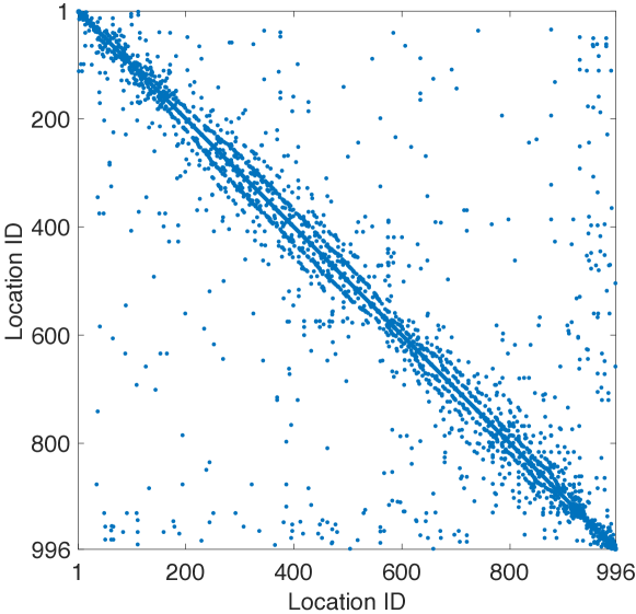
Figure 5: Structure of the conditional correlation matrix (under a threshold of 0.1; each dot represents a non-zero entry).

Table 1: RMSE and MAPE of Forecaster and baseline models.

Metrics	Model	Average	Next step	Second next step	Third next step
	VAR	6.9991	6.4243	7.1906	7.3476
	DCRNN	5.3750 ± 0.0691	5.1627 ± 0.0644	5.4018 ± 0.0673	5.5532 ± 0.0758
RMSE	Transformer (same width)	5.6802 ± 0.0206	5.4055 ± 0.0109	5.6632 ± 0.0173	5.9584 ± 0.0478
	Transformer (best width)	5.6898 ± 0.0219	5.4066 ± 0.0302	5.6546 ± 0.0581	5.9926 ± 0.0472
	Forecaster	5.1879 ± 0.0082	4.9629 ± 0.0102	5.2275 ± 0.0083	5.3651 ± 0.0065
	VAR	33.7983	31.9485	34.5338	34.9126
	DCRNN	24.9853 ± 0.1275	24.4747 ± 0.1342	25.0366 ± 0.1625	25.4424 ± 0.1238
MAPE (%)	Transformer (same width)	22.5787 ± 0.2153	21.8932 ± 0.2006	22.3830 ± 0.1943	23.4583 ± 0.2541
	Transformer (best width)	22.2793 ± 0.1810	21.4545 ± 0.0448	22.1954 ± 0.1792	23.1868 ± 0.3334
	Forecaster	20.1362 ± 0.0316	19.8889 ± 0.0269	20.0954 ± 0.0299	20.4232 ± 0.0604

Our evaluation of Forecaster starts by using Gaussian Markov random fields to determine the spatial dependency between the data at different locations. Based on the method in Section 2.2, we can obtain a conditional correlation matrix where each entry of the matrix represents the conditional correlation coefficient between two locations. If the absolute value of an entry is less than a threshold, we will treat the corresponding two locations as conditionally independent, and round the value of the entry to zero. This threshold can be chosen based only on the performance on the validation set. Figure 5 shows the structure of the conditional correlation matrix under a threshold of 0.1. We can see that the matrix is sparse, which means a location generally depends on just a few other locations other than all the locations. We found that a location depends on only 2.5 other locations on average. There are some locations which many other locations depend on. For example, there is a location in Lower Manhattan which 16 other locations depend on. This may be because there are many locations with significant taxi demand in Lower Manhattan, with these locations sharing a strong dependency. Figure 6 shows the top 400 spatial dependencies. We see some long-range spatial dependency between remote locations. For example, there is a strong dependency between Grand Central Terminal and New York Penn Station, which are important stations in Manhattan with a large traffic of passengers.

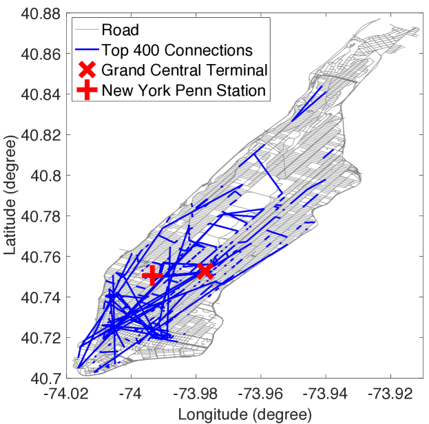
Figure 6: Top 400 dependency relations between locations.

After determining the spatial dependency between locations, we use the graph Transformer architecture of Forecaster to predict the taxi demand. Table 1 contrasts the performance of Forecaster to other baseline models. Here we run all the evaluated deep learning models six times (using different seeds) and report the mean and the standard deviation of the results. As VAR is not subject to the impact of random initialization, we run it once. We can see for all the evaluated models, the RMSE and MAPE of predicting the next step are lower than that of predicting later steps (e.g., the third next step). This is because, for all the models, the prediction of later steps is built upon the prediction of the next step, and thus the error of the former includes the error of the latter. Comparing the performance of these models, we can see the RMSE and MAPE of VAR is higher than that of the deep learning models. This is because VAR does not model well the non-linearity and non-stationarity within the data; it also does not consider the spatial dependencies between locations in the structure of its coefficient matrices (matrices $A_{i}$ and $B$ in Equation (8)). Among the deep learning models, DCRNN and the Transformer perform similarly. The former captures the spatial dependency within the data but does not capture well the long-range temporal dependency, while the latter focuses on exploiting the long-range temporal dependency but neglects the spatial dependency. As for our method, Forecaster outperforms all the baseline methods at every future step of forecasting. On average (over these future steps), Forecaster achieves an RMSE of 5.1879 and a MAPE of 20.1362, which is 8.8210% and 9.6192% better than Transformer (best width), and 3.4809% and 19.4078% better than DCRNN. This demonstrates the advantage of Forecaster in capturing both the spatial dependency and the long-range temporal dependency.

4 Related Work

To our knowledge, this work is the first (1) to integrate Gaussian Markov Random fields with deep learning to forecast spatial and time-dependent data, using the former to derive a dependency graph; (2) to sparsify the architecture of the Transformer based on the dependency graph, significantly improving the forecasting quality of the result architecture. The most closely related work is a set of proposals on forecasting spatial and time-dependent data and the Transformer, which we briefly review in this section.

4.1 Spatial and Time-Dependent Data Forecasting

Conventional methods for forecasting spatial and time-dependent data such as ARIMA and Kalman filtering-based methods [18, 17] usually impose strong stationary assumptions on the data, which are often violated [16]. Recently, deep learning-based methods have been proposed to tackle the non-stationary and highly nonlinear nature of the data [35, 38, 36, 7, 34, 16]. Most of these works consist of two parts: modules to capture spatial dependency and modules to capture temporal dependency. Regarding spatial dependency, the literature mostly uses prior knowledge such as physical closeness between regions to derive an adjacency matrix and/or pre-defined distance/similarity metrics to decide whether two locations are dependent or not. Then, based on this information, they usually use a (standard or graph) CNN to characterize the spatial dependency between dependent locations. However, these methods are not good predictors of dependency relations between the data at different locations. Regarding temporal dependency, available works [35, 36, 7, 34, 16] usually use RNNs and CNNs to extract the long-range temporal dependency. However, both RNN and CNN do not learn well the long-range temporal dependency, with the number of operations used to relate signals at two distant time positions in a sequence growing at least logarithmically with the distance between them [29].

We evaluate our architecture with the problem of forecasting taxi ride-hailing demand around a large number of spatial locations. The problem has two essential features: (1) These locations are not uniformly distributed like pixels in an image, making standard CNN-based methods [35, 34, 38] not good for this problem; (2) it is desirable to perform multi-step forecasting, i.e., forecasting at several time instants in the future, this implying that the work mainly designed for single-step forecasting [36, 7] is less applicable. DCRNN [16] is the state-of-the-art baseline satisfying both features. Hence, we compare our architecture with DCRNN and show that our work outperforms DCRNN.

4.2 Transformer

The Transformer [29] avoids recurrence and instead purely relies on the self-attention mechanism to let the data at distant positions in a sequence to relate to each other directly. This benefits learning long-range temporal dependency. The Transformer and its extensions have been shown to significantly outperform RNN-based methods in NLP and image generation tasks [29, 22, 3, 33, 4, 21, 13]. It has also been applied to graph and node classification problems [1, 37]. However, it is still unknown how to apply the architecture of Transformer to spatial and time-dependent data, especially to deal with spatial dependency between locations. Later work [31] extends the architecture of Transformer to video generation. Even though this also needs to address spatial dependency between pixels, the nature of the problem is different from our task. In video generation, pixels exhibit spatial dependency only over a short time interval, lasting for at most tens of frames — two pixels may be dependent only for a few frames and become independent in later frames. On the contrary, in spatial and time-dependent data, locations exhibit long-term spatial dependency lasting for months or even years. This fundamental difference of the applications that we consider enables us to use Gaussian Markov random fields to determine the dependency graph as basis for sparsifying the Transformer. Child et al. [2] propose another sparse Transformer architecture with a different goal of accelerating the multi-head attention operations in the Transformer. This architecture is very different from our architecture.

5 Conclusion

Forecasting spatial and time-dependent data is challenging due to complex spatial dependency, long-range temporal dependency, non-stationarity, and heterogeneity within the data. This paper proposes Forecaster, a graph Transformer architecture to tackle these challenges. Forecaster uses Gaussian Markov random fields to determine the dependency graph between the data at different locations. Then, Forecaster sparsifies the architecture of the Transformer based on the structure of the graph and lets the sparsified Transformer (i.e., graph Transformer) capture the spatiotemporal dependency, non-stationarity, and heterogeneity in one shot. We apply Forecaster to the problem of forecasting taxi-ride hailing demand at a large number of spatial locations. Evaluation results demonstrate that Forecaster significantly outperforms state-of-the-art baselines (the Transformer and DCRNN). We thank the reviewers. This work is partially supported by NSF CCF (award 1513936).

Appendix: Multi-Head Attention

The multi-head attention layer is a core component of the Transformer for capturing long-range temporal dependency within data. It takes a query sequence $\left\{\mathbf{{q}}_{t}\mid\mathbf{{q}}_{t}\in\mathbb{{R}}^{d_{model}},\>t=1,\ldots,T\right\}$, a key sequence $\left\{\mathbf{{k}}_{t}\mid\mathbf{{k}}_{t}\in\mathbb{{R}}^{d_{model}},\>t=1,\ldots,T\right\}$, and a value sequence $\left\{\mathbf{{v}}_{t}\mid\mathbf{{v}}_{t}\in\mathbb{{R}}^{d_{model}},\>t=1,\ldots,T\right\}$ as inputs, and outputs a new sequence $\left\{\mathbf{{e}}_{t}\mid\mathbf{{e}}_{t}\in\mathbb{{R}}^{d_{model}},\>t=1,\ldots,T\right\}$ where each element of the output sequence is impacted by the corresponding query and all the keys and values, no matter how distant these keys and values are from the query in the temporal order, and thus captures the long-range temporal dependency. The detailed procedure is as follows.

First, the multi-head attention layer compares each query $\mathbf{q}_{t}$ with each key $\mathbf{k}_{j}$ to get their similarity $\alpha_{tj}^{(h)}$ from multiple perspectives (termed as multi-head; $H$ is the number of heads, $h=1,\ldots,H$):

$$\begin{array}[]{rcl}\alpha_{tj}^{(h)}&=&\mathrm{{softmax}}\left(\left\langle W_{(h)}^{Q}\mathbf{q}_{t},\>W_{(h)}^{K}\mathbf{k}_{j}\right\rangle\Big{/}\sqrt{\frac{d_{model}}{H}}\right)\\ \\ \large\hfil&=&\dfrac{\mathrm{{exp}}\left(\left\langle W_{(h)}^{Q}\mathbf{q}_{t},\>W_{(h)}^{K}\mathbf{k}_{j}\right\rangle\Big{/}\sqrt{\frac{d_{model}}{H}}\right)}{\sum\limits_{i=1}^{T}\mathrm{{exp}}\left(\left\langle W_{(h)}^{Q}\mathbf{q}_{t},\>W_{(h)}^{K}\mathbf{k}_{i}\right\rangle\Big{/}\sqrt{\frac{d_{model}}{H}}\right)}\end{array}$$ (9)

where $\alpha_{ij}^{(h)}\in\left(0,\>1\right)$ is the similarity between $\mathbf{q}_{i}$ and $\mathbf{k}_{j}$ under head $h$, $\sum_{j=1}^{T}\alpha_{ij}^{(h)}=1$; $W_{(h)}^{Q},W_{(h)}^{K}\in\mathbb{{R}}^{\frac{d_{model}}{H}\times d_{model}}$ are parameter matrices for head $h$ that need to be learned; $\left\langle\cdot,\>\cdot\right\rangle$ is the inner product between two vectors.

In our work, to balance the impact of spatial signals and auxiliary information on the prediction, we first scale $\mathbf{{q}}_{t}$ and then use its scaled version $\mathbf{{q}}_{t}^{\prime}$ instead in Equation (9) for computing the similarity $\alpha_{tj}^{(h)}$. Suppose in $\mathbf{{q}}_{t}$ and $\mathbf{{k}}_{t}$, the first $d_{signal}$ dimensions are for encoding spatial signals, and the next $d_{aux}$ dimensions are for encoding auxiliary information, we compute $\mathbf{{q}}_{t}^{\prime}$ as:

$$\begin{array}[]{c}\mathbf{{q}}_{t}^{\prime}=\mathbf{{r}}\circ\mathbf{{q}}_{t}\\ \\ \mathbf{{r}}=\left[\begin{array}[]{c}\sqrt{\frac{1}{2}+\frac{d_{aux}}{2d_{signal}}}\cdot\mathbf{{1}}_{d_{signal}},\;\sqrt{\frac{1}{2}+\frac{d_{signal}}{2d_{aux}}}\cdot\mathbf{{1}}_{d_{aux}}\end{array}\right]^{{\rm{T}}}\\ \\ \mathbf{{1}}_{d}=\left[\begin{array}[]{ccc}1&\cdots&1\end{array}\right]\in\mathbb{{R}}^{1\times d},\quad d=d_{signal}\;\textrm{{or}}\;d_{aux}\end{array}$$ (10)

where $\circ$ is the Hadamard product.

Second, the multi-head attention layer uses these similarities as weights to generate a new sequence $\left\{\mathbf{{e}}_{t}^{(h)}\mid\mathbf{{e}}_{t}^{(h)}\in\mathbb{{R}}^{d_{model}},\>t=1,\ldots,T\right\}$ for each head $h$:

$$\mathbf{{e}}_{t}^{(h)}=\sum_{j=1}^{T}\alpha_{tj}^{(h)}W_{(h)}^{V}\mathbf{v}_{j}$$ (11)

where $W_{(h)}^{V}\in\mathbb{{R}}^{\frac{d_{model}}{H}\times d_{model}}$ is another parameter matrix for head $h$ that needs to be learned.

Third, the sequence under each head is concatenated and then used to generate the final output sequence:

$$\mathbf{{e}}_{t}=W^{O}\left[\mathbf{{e}}_{t}^{(1)}\bigparallel\mathbf{{e}}_{t}^{(2)}\bigparallel\cdots\bigparallel\mathbf{{e}}_{t}^{(H)}\right]$$ (12)

where $W^{O}\in\mathbb{{R}}^{d_{model}\times d_{model}}$ is a parameter matrix that needs to be learned; $\cdot\bigparallel\cdot$ represents a concatenation of two vectors.

In summary, the multi-head attention layer needs to learn the parameter matrices $W_{(h)}^{Q}$, $W_{(h)}^{K}$, $W_{(h)}^{V}$, $h=1,\cdots,H$, and $W^{O}$, which all can be treated as linear layers without bias. In our architecture, we use sparse linear layers to replace these linear layers, capturing the spatial dependency between locations.

References

- [1] Benson Chen, Regina Barzilay, and Tommi Jaakkola, ‘Path-Augmented Graph Transformer Network’, in Workshop on Learning and Reasoning with Graph-Structured Data (ICML workshop), pp. 1–5, (2019).
- [2] Rewon Child, Scott Gray, Alec Radford, and Ilya Sutskever, ‘Generating Long Sequences with Sparse Transformers’, arXiv preprint arXiv:1904.10509, (2019).
- [3] Zihang Dai, Zhilin Yang, Yiming Yang, William W Cohen, Jaime Carbonell, Quoc V Le, and Ruslan Salakhutdinov, ‘Transformer-XL: Attentive Language Models beyond a Fixed-Length Context’, in Annual Meeting of the Association for Computational Linguistics (ACL), pp. 2978–2988, (2019).
- [4] Jacob Devlin, Ming-Wei Chang, Kenton Lee, and Kristina Toutanova, ‘Bert: Pre-training of Deep Bidirectional Transformers for Language Understanding’, in Annual Conference of the North American Chapter of the Association for Computational Linguistics: Human Language Technologies (NAACL-HLT), p. 4171–4186, (2019).
- [5] Jian Du, Shanghang Zhang, Guanhang Wu, José M. F. Moura, and Soummya Kar, ‘Topology Adaptive Graph Convolutional Networks’, arXiv preprint arXiv:1710.10370, 1–13, (2017).
- [6] Jerome Friedman, Trevor Hastie, and Robert Tibshirani, ‘Sparse Inverse Covariance Estimation with the Graphical Lasso’, Biostatistics, 9(3), 432–441, (2008).
- [7] Xu Geng, Yaguang Li, Leye Wang, Lingyu Zhang, Qiang Yang, Jieping Ye, and Yan Liu, ‘Spatiotemporal Multi-Graph Convolution Network for Ride-Hailing Demand Forecasting’, in AAAI Conference on Artificial Intelligence, pp. 3656–3663, (2019).
- [8] Alfred Greiner, Willi Semmler, and Gang Gong, The Forces of Economic Growth: A Time Series Perspective, Princeton University Press, 2016.
- [9] Sepp Hochreiter, Yoshua Bengio, Paolo Frasconi, and Jürgen Schmidhuber, Gradient Flow in Recurrent Nets: the Difficulty of Learning Long-Term Dependencies, A Field Guide to Dynamical Recurrent Neural Networks. IEEE Press, 2001.
- [10] Johannes Hofmann, Michael Größler, Manuel Rubio-Sánchez, P-P Pichler, and Dirk Joachim Lehmann, ‘Visual Exploration of Global Trade Networks with Time-Dependent and Weighted Hierarchical Edge Bundles on GPU’, Computer Graphics Forum, 36(3), 273–282, (2017).
- [11] Ashesh Jain, Amir R Zamir, Silvio Savarese, and Ashutosh Saxena, ‘Structural-RNN: Deep Learning on Spatio-Temporal Graphs’, in IEEE Conference on Computer Vision and Pattern Recognition (CVPR), pp. 5308–5317, (2016).
- [12] Thomas N. Kipf and Max Welling, ‘Semi-Supervised Classification with Graph Convolutional Networks’, in International Conference on Learning Representations (ICLR), pp. 1–14, (2017).
- [13] Rik Koncel-Kedziorski, Dhanush Bekal, Yi Luan, Mirella Lapata, and Hannaneh Hajishirzi, ‘Text Generation from Knowledge Graphs with Graph Transformers’, in Annual Conference of the North American Chapter of the Association for Computational Linguistics: Human Language Technologies (NAACL-HLT), pp. 2284–2293, (2019).
- [14] Jie Li, Siming Chen, Kang Zhang, Gennady Andrienko, and Natalia Andrienko, ‘Cope: Interactive Exploration of Co-Occurrence Patterns in Spatial Time Series’, IEEE Transactions on Visualization and Computer Graphics, 25(8), 2554–2567, (2019).
- [15] Jie Li, Kang Zhang, and Zhao-Peng Meng, ‘Vismate: Interactive Visual Analysis of Station-Based Observation Data on Climate Changes’, in IEEE Conference on Visual Analytics Science and Technology (VAST), pp. 133–142, (2014).
- [16] Yaguang Li, Rose Yu, Cyrus Shahabi, and Yan Liu, ‘Diffusion Convolutional Recurrent Neural Network: Data-Driven Traffic Forecasting’, in International Conference on Learning Representations (ICLR), pp. 1–16, (2018).
- [17] Marco Lippi, Matteo Bertini, and Paolo Frasconi, ‘Short-Term Traffic Flow Forecasting: An Experimental Comparison of Time-Series Analysis and Supervised Learning’, IEEE Transactions on Intelligent Transportation Systems, 14(2), 871–882, (2013).
- [18] Wei Liu, Yu Zheng, Sanjay Chawla, Jing Yuan, and Xie Xing, ‘Discovering Spatio-Temporal Causal Interactions in Traffic Data Streams’, in ACM SIGKDD International Conference on Knowledge Discovery and Data Mining (KDD), pp. 1010–1018, (2011).
- [19] Helmut Lütkepohl, New Introduction to Multiple Time Series Analysis, Springer, 2005.
- [20] Daniel B Neill, ‘Expectation-Based Scan Statistics for Monitoring Spatial Time Series Data’, International Journal of Forecasting, 25(3), 498–517, (2009).
- [21] Niki Parmar, Ashish Vaswani, Jakob Uszkoreit, Lukasz Kaiser, Noam Shazeer, Alexander Ku, and Dustin Tran, ‘Image Transformer’, in International Conference on Machine Learning (ICML), pp. 4055–4064, (2018).
- [22] Alec Radford, Karthik Narasimhan, Tim Salimans, and Ilya Sutskever, ‘Improving Language Understanding by Generative Pre-training’, OpenAI, (2018).
- [23] Pradeep Ravikumar, Martin J Wainwright, Garvesh Raskutti, and Bin Yu, ‘High-Dimensional Covariance Estimation by Minimizing L1-Penalized Log-Determinant Divergence’, Electronic Journal of Statistics, 5, 935–980, (2011).
- [24] Havard Rue and Leonhard Held, Gaussian Markov Random Fields: Theory And Applications (Monographs on Statistics and Applied Probability), Chapman & Hall/CRC, 2005.
- [25] Skipper Seabold and Josef Perktold, ‘Statsmodels: Econometric and Statistical Modeling with Python’, in Python in Science Conference, pp. 57–61, (2010).
- [26] John Shi, Mark Cheung, Jian Du, and José M. F. Moura, ‘Classification with Vertex-Based Graph Convolutional Neural Networks’, in Asilomar Conference on Signals, Systems, and Computers (ACSSC), pp. 752–756, (2018).
- [27] Ilya Sutskever, Oriol Vinyals, and Quoc V Le, ‘Sequence to Sequence Learning with Neural Networks’, in Advances in Neural Information Processing Systems (NIPS), pp. 3104–3112, (2014).
- [28] NYC Taxi and Limousine Commission, ‘Trip Record Data’, (2018).
- [29] Ashish Vaswani, Noam Shazeer, Niki Parmar, Jakob Uszkoreit, Llion Jones, Aidan N Gomez, Lukasz Kaiser, and Illia Polosukhin, ‘Attention is All You Need’, in Advances in Neural Information Processing Systems (NIPS), pp. 5998–6008, (2017).
- [30] Jacob Walker, Kenneth Marino, Abhinav Gupta, and Martial Hebert, ‘The Pose Knows: Video Forecasting by Generating Pose Futures’, in IEEE International Conference on Computer Vision (ICCV), pp. 3332–3341, (2017).
- [31] Xiaolong Wang, Ross B. Girshick, Abhinav Gupta, and Kaiming He, ‘Non-Local Neural Networks’, in IEEE Conference on Computer Vision and Pattern Recognition (CVPR), pp. 7794–7803, (2018).
- [32] Weather Underground, ‘Historical Weather’, (2018).
- [33] Zhilin Yang, Zihang Dai, Yiming Yang, Jaime Carbonell, Ruslan Salakhutdinov, and Quoc V Le, ‘XLNet: Generalized Autoregressive Pretraining for Language Understanding’, arXiv preprint arXiv:1906.08237, (2019).
- [34] Huaxiu Yao, Xianfeng Tang, Hua Wei, Guanjie Zheng, and Zhenhui Li, ‘Revisiting Spatial-Temporal Similarity: A Deep Learning Framework for Traffic Prediction’, in AAAI Conference on Artificial Intelligence, pp. 5668–5675, (2019).
- [35] Huaxiu Yao, Fei Wu, Jintao Ke, Xianfeng Tang, Yitian Jia, Siyu Lu, Pinghua Gong, Jieping Ye, and Zhenhui Li, ‘Deep Multi-View Spatial-Temporal Network for Taxi Demand Prediction’, in AAAI Conference on Artificial Intelligence, pp. 2588–2595, (2018).
- [36] Bing Yu, Haoteng Yin, and Zhanxing Zhu, ‘Spatio-Temporal Graph Convolutional Networks: A Deep Learning Framework for Traffic Forecasting’, in International Joint Conference on Artificial Intelligence (IJCAI), pp. 3634–3640, (2018).
- [37] Seongjun Yun, Minbyul Jeong, Raehyun Kim, Jaewoo Kang, and Hyunwoo J Kim, ‘Graph Transformer Networks’, in Advances in Neural Information Processing Systems (NeurIPS), pp. 11960–11970, (2019).
- [38] Junbo Zhang, Yu Zheng, and Dekang Qi, ‘Deep Spatio-Temporal Residual Networks for Citywide Crowd Flows Prediction’, in AAAI Conference on Artificial Intelligence, pp. 1655–1661, (2017).
- [39] Pusheng Zhang, Yan Huang, Shashi Shekhar, and Vipin Kumar, ‘Correlation Analysis of Spatial Time Series Datasets: A Filter-and-Refine Approach’, in Pacific-Asia Conference on Knowledge Discovery and Data Mining (PAKDD), pp. 532–544, (2003).
- [40] Ali Ziat, Edouard Delasalles, Ludovic Denoyer, and Patrick Gallinari, ‘Spatio-Temporal Neural Networks for Space-Time Series Forecasting and Relations Discovery’, in IEEE International Conference on Data Mining (ICDM), pp. 705–714, (2017).