Hypergraph Partitioning With Embeddings

Hypergraph Partitioning with Embeddings

Abstract

Problems in scientific computing, such as distributing large sparse matrix operations, have analogous formulations as hypergraph partitioning problems. A hypergraph is a generalization of a traditional graph wherein “hyperedges” may connect any number of nodes. As a result, hypergraph partitioning is an NP-Hard problem to both solve or approximate. State-of-the-art algorithms that solve this problem follow the multilevel paradigm, which begins by iteratively “coarsening” the input hypergraph to smaller problem instances that share key structural features. Once identifying an approximate problem that is small enough to be solved directly, that solution can be interpolated and refined to the original problem. While this strategy represents an excellent trade off between quality and running time, it is sensitive to coarsening strategy. In this work we propose using graph embeddings of the initial hypergraph in order to ensure that coarsened problem instances retrain key structural features. Our approach prioritizes coarsening within self-similar regions within the input graph, and leads to significantly improved solution quality across a range of considered hypergraphs.
Reproducibility: All source code, plots and experimental data are available at https://sybrandt.com/2019/partition.

1 Introduction

Hypergraphs provide the formalism needed to solve problems consisting of interconnected item sets. Similar to a traditional graph, the hypergraph has the added generalization that “hyperedges” may connect any number of nodes. Domains such as very-large-scale integration for creating integrated circuits [25], machine learning [55, 20, 53], parallel algorithms [11], combinatorial scientific computing [21], and social network analysis [43, 54] all contain significant and challenging instances of hypergraph problems. One important problem, Hypergraph partitioning, involves dividing the nodes of a hypergraph among $k$ similarly-sized disjoint sets while reducing the number of hyperedges that span multiple partitions. In the context of load balancing, this is the problem of dividing logical threads (nodes) that share data dependencies (hyperedges) among available machines (partitions) in order to balance the number of threads per machine and minimize communication overhead. However, hypergraph partitioning is both NP-Hard to solve [29] and approximate [7].

Therefore, state-of-the-art partitioners apply heuristically-backed algorithms to overcome these inherent computational limitations [8]. The most common and effective technique is the multilevel paradigm [2, 41, 25, 5, 14]. The multilevel paradigm is well known to be successful beyond the (hyper)graph partitioning in such areas as the cut-based problems on graphs [37] and machine learning [36]. Multilevel partitioners consist of three phases, referred to collectively as the V-Cycle: coarsening, the initial solution, and uncoarsening. We depict these phases in Figure 1. The overarching idea behind this technique is to find a problem instance that shares key structural features with the input hypergraph, but is small enough to be partitioned directly. The initial solution to this small analogous problem can then be gradually interpolated and refined to apply to the input hypergraph.

The small analogous problem is identified through an iterative coarsening process consisting of many levels. At each level, groups of similar nodes are identified, and each is “contracted” into a single merged node at the next more-coarse level. While grouping nodes, the goal is to identify self-similar regions of the current hypergraph so that the more coarse problem instances retain key structural features. Most commonly, these coarsening groups are formed by pairing nodes due to a similarity measure [14, 41] that heuristically or rigorously suggests to place both nodes in the same partition. An $n$-level algorithm is one that identifies only one pair of coarsening partners at each level [40], while a $\log n$-level algorithm pairs many nodes each time [14]. Coarsening stops once identifying a sufficiently small hypergraph based on some criterion that indicates that this problem is possible to (almost) optimally solve on given computational resources. The initial solution can then be identified directly using the best available algorithm. Now, the solution is uncoarsened back through the levels in order to identify a solution to the original problem. Uncoarsening consists of three sub-phases: expansion, interpolation, and refinement. Expansion undoes the coarsening at a given level by “expanding” the current level’s coarsened nodes with those contracted in the prior. Next, interpolation assigns each expanded node the partition label assigned to their corresponding coarse representation. Then, local refinement cheaply updates the partition labels among the expanded nodes in order to improve the overall solution quality for the next level. This process is repeated from the initial solution through all coarsening levels and back to the original hypergraph, which final refinement solution is accepted as the solution to the partitioning problem.

Because the strategy used to contract nodes determines the coarsening at each level, the quality of the initial solution, and the behavior of interpolation and refinement during uncoarsening, we find that this single factor can dramatically effect partitioning quality. Other works exploring coarsening strategies, such as relaxation-based [41] or community-aware [23] coarsening, arrive with a similar conclusion.

1.1 Our Contribution

We propose embedding-based coarsening, a novel coarsening strategy that leverages graph embeddings to prioritize the contraction of self-similar regions of the input hypergraph in order to retain global structural features. This approach augments the existing strategy that contracts nodes based on their co-participation in small hyperedges by adding an embedding-based term that can break ties among similarly ranked coarsening pairs. A toy example of this phenomena is depicted in Figure 2, wherein three potential coarsening pairs are equally ranked by the traditional scheme, but embedding-based signals favor the pair that retains both key clusters.

The field of graph embedding is evolving rapidly, and the proposed embedding-based coarsening is designed to be agnostic with respect to any particular technique, provided that similarities between nodes are encoded via the dot product of embedding vectors. Specifically, our proposed technique accepts a precomputed embedding as an auxiliary input per-hypergraph, and we demonstrate that a wide range of existing embedding techniques improve partitioning performance similarly. Decoupling partitioning from embedding enables embedding-based coarsening to more easily benefit from future advances in machine learning techniques. In order to apply embedding techniques designed for classical graphs, we need a classical representation of each input hypergraph. The star-expansion [1] represents a hypergraph as an undirected bipartite graph wherein hyperedges from the original structure form a new layer of nodes. An edge between two nodes $i$ and $j$ in the bipartite structure indicates that node $i$ participated in hyperedge $j$ within the original structure. As opposed to other classical representations like the clique-expansion, the star-expansion retains all relevant hypergraph information, and is scalable for large graphs [1]. Furthermore, existing embedding techniques specifically designed for bipartite graphs [45] apply to star-expanded graphs directly.

Given an input hypergraph and an embedding for each node of the input structure, embedding-based coarsening follows this outline at each coarsening level. First, each node is assigned a score equal to the highest dot product between its embedding and each of its neighbors. Nodes are visited in decreasing order by score. A visited node is matched from among its neighbors based on the product of their classical edge-wise score, and the dot product of each node’s embedding. After matching nodes, based on whether we are performing $n$- or $\log n$-level coarsening, mated nodes are contracted. Newly coarsened nodes are assigned an embedding equal to the average embedding of all initial embeddings contained within the coarse representation.

We implement our proposed coarsening strategy in both KaHyPar [40], which is a $n$-level partitioner with state-of-the-art solution quality, as well as Zoltan [14], which is a parallel $\log n$-level partitioner with high quality and state-of-the-art speed. Furthermore, we compare the effect of various different embedding techniques, including Node2Vec [19], Metapath2Vec++ [15], and FOBE/HOBE [45], which were designed specifically for bipartite graphs. We additionally compare the effect of each embedding-based coarsening strategy with hMetis [24], Zoltan [14], PaToH [10], KaHyPar (with community-based coarsening [23]), and KaHyPar Flow (with both community-based coarsening and flow-based refinement [22]). We compare performance of each partitioner across 96 hypergraph from the SuiteSparse Matrix Collection [13]. For each graph, we compute one embedding using each of the proposed techniques to serve as an auxiliary input across all trial. We compare quality across both the “cut” and “connectivity” objectives as well as for partition counts from 2 to 128 for each partitioner. For each combination of experimental parameters we run 20 trials in order to compare the variance and establish significance with respect to different random seeds. Overall, we produce over 500,000 individual trials.

We find that embedding-based coarsening has a significant improvement over the state of the art that is especially pronounced for smaller partition counts ($<32$). In some cases, this leads to a solution quality that is improved by as much as $400\%$. Because embedding-based coarsening replaces the traditionally random visit order with one that prioritizes self-similar regions of the hypergraph, we also observe an improvement in the standard deviation of quality. All experimental code, data, visualization scripts, and a database of all experimental results, including all hyperparameters per-trial, can be found at: https://sybrandt.com/2019/partition. A longer-form version of this work can be found online.

Figure 1: A standard V-cycle, consisting of coarsening, and initial partition, and uncoarsening.

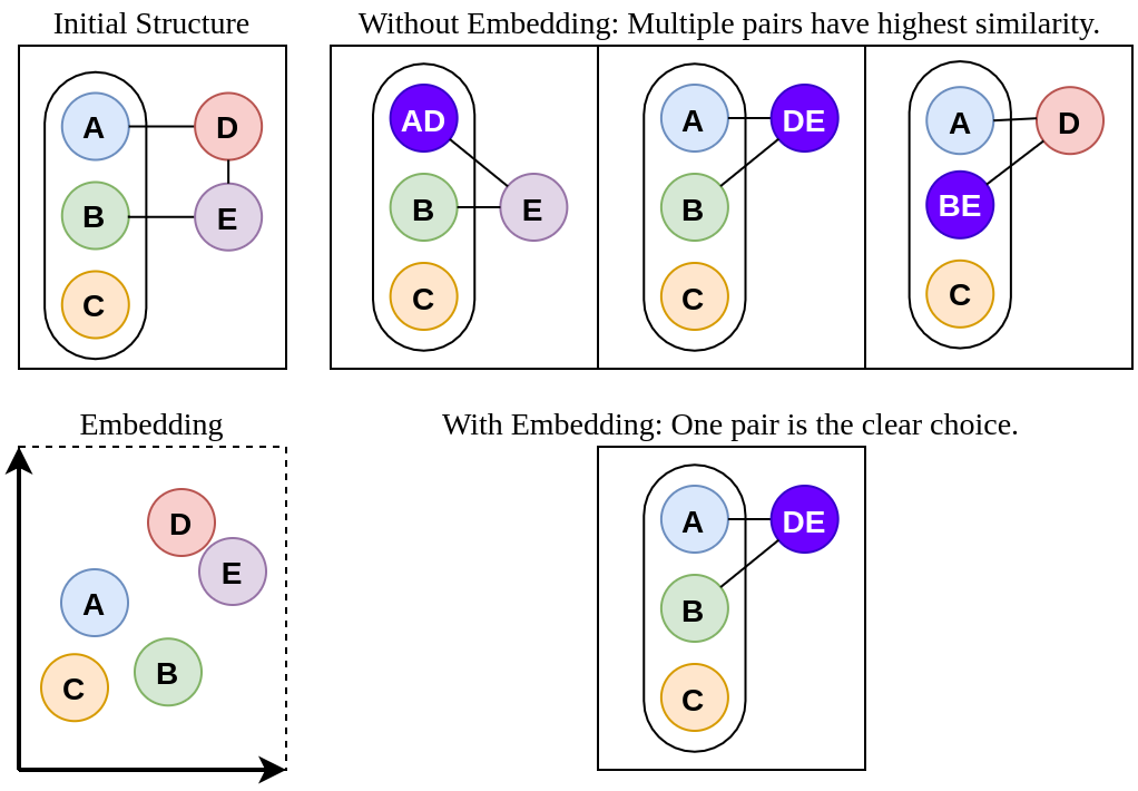
Figure 2: Typical heavy-edge coarsening results in three possible contractions of equal weight. Embedding-based coarsening breaks the tie for the pair that preserves global structure — a cluster of weight 3 and of weight 2.

2 Notation and Preliminary Concepts

A hypergraph $H=(V,E)$ consists of nodes $v\in V$ and hyperedges $e\in E$. As opposed to a traditional graph, each hyperedge may contain any non-empty subset of $V$. The hypergraph partitioning problem is to divide $V$ into $k$ disjoint subsets of similar size while minimizing a given objective function. Two common objectives considered here are “cut” and “connectivity.” Cut measures the number of hyperedges spanning more than one partition. If $\lambda(e)$ is the number of partitions spanned by edge $e$, then the cut objective is defined as: ${|e\in E,\text{ such that }\lambda(e)>1|}$.

The “connectivity” objective, also commonly referred to as “$k-1$,” penalizes each edge by the number of spanned partitions, namely, ${\sum_{e\in E}(\lambda(e)-1})$. In the case of $k=2$, this is equivalent to cut.

Weights. Although we consider unweighted input hypergraphs (all nodes and hyperedges count the same towards their corresponding objectives and constraints), the multilevel paradigm introduces weights to intermediate level hypergraphs. Each node and hyperedge has a corresponding weight ($w_{v}$ and $w_{e}$) equal to one for the input hypergraph. During coarsening, if two nodes $v_{i}$ and $v_{j}$ are contracted into a new coarse node $v^{\prime}$, then $w_{v^{\prime}}=w_{v_{i}}+w_{v_{j}}$. This new node $v^{\prime}$ will also be added to all edges originally containing either $v_{i}$ or $v_{j}$, before removing those original nodes from the resulting coarse hypergraph. If during the coarsening two edges will contain the same subset of nodes ($e_{1}=e_{2}$), they will be replaced with a new edge $e^{\prime}$ containing the same nodes but with added weights: $w_{e^{\prime}}=w_{e_{1}}+w_{e_{2}}$. When solving for cut and connectivity for intermediate sub-problems during the multilevel strategy, we introduce these weights into the objective:

$$\text{weighted cut}=\sum_{e\in E,\lambda(e)>1}w_{e}$$ (1)

$$\text{weighted connectivity}=\sum_{e\in E}(\lambda(e)-1)w_{e}$$ (2)

One issue during coarsening is the potential for individual nodes to accumulate a disproportionate amount of weight. When this occurs, balanced partitioning can become impossible at the coarsest level, especially if one node’s weight exceeds $|V|/k$. In order to avoid this negative effect, multilevel partitioners enforce a weight tolerance $w^{(T)}$, which is parameterized by the user. No coarsening partners may be contracted if their resulting coarse node would exceed this limit.

Imbalance Constraint. It is important to balance the number of nodes in the resulting partitions. Therefore, partitioners include an optimization constraint to determine how uneven the resulting partitions are allowed to be. For each partition $V_{i}\subset V$, given a predefined imbalance tolerance $\alpha$, this constraint is defined as:

$$\sum_{v^{\prime}\in V_{i}}w_{v^{\prime}}\leq(1+\alpha)\left\lceil\frac{1}{k}\sum_{v\in V}w_{v}\right\rceil$$ (3)

Embeddings. We use the function $\epsilon:V\rightarrow\mathbb{R}^{n}$ to denote a pre-trained embedding. Conceptually, this is a lookup table that assigns a node in the input hypergraph to a real-valued $n$-dimensional vector. In our experiments we select $n=100$. Note, higher-dimensional embeddings show no statistically significant performance difference in our experiments.

3 Background and Related Work

Multilevel Partitioning. First introduced to speed up existing algorithms [3] and inspired by multigrid and multiscale optimization strategies [6], the multilevel method was quickly recognized as an effective approach to improve the quality of (hyper)graph partitioning [26], and is currently considered to be one of the state-of-the-art methods for this problem [8]. As introduced in Section 1, the basic version of the multilevel paradigm solves problems by following the V-cycle pattern that consists of coarsening, the initial solution, and uncoarsening. This approach is effective because coarse hypergraphs are easier to solve yet they retain global structural features of the original. Coarse hypergraphs are created by iteratively merging multiple nodes at the current “finer” level into single nodes at the “coarser” level. Once sufficiently small, a partitioner can directly solve the coarsest problem instance using an algorithm that would normally be infeasible for large problems. The uncoarsening process then applies that solution through iteratively finer problem instances by expanding contracted nodes, interpolating coarse solutions onto finer problem instances, and refining intermediate solutions at each level. Once the uncoarsening process reaches the most-fine problem instance, the refined solution is accepted as the partitioning of the input hypergraph.

Usually, at each level of the coarsening process almost all nodes have at least one merging partner, resulting in $\log n$ levels. This is the approach used by Mondriaan [51], hMetis2 [25], Zoltan [14], and PaToH [10]. However, KaHyPar [40] implements an $n$-level approach where at each level only one pair of nodes is contracted. The multilevel paradigm is the current gold-standard for hypergraph partitioning, having achieved an excellent trade off between time and quality. Unsurprisingly, most practical and state-of-the-art partitioners follow this paradigm, including all methods considered in this work. For an extensive review of (hyper)graph partitioning methods, we refer the reader to [8, 4].

Coarsening Strategies. Multilevel partitioners follow heuristic strategies to identify groups of nodes to contract during coarsening. A good coarsening strategy is one that groups together nodes that will ultimately share the same partition label, meaning that the coarser solution can be interpolated to the finer solution without a loss of quality. In practice, this loss of quality is to be expected, which is why local refinement is common during uncoarsening. However, if global structural features are not preserved, the loss of quality during interpolation cannot be rectified through the fast local refinement process. Therefore, the choice of coarsening heuristic is paramount.

Most heuristics used to identify nodes for contraction do so by scoring node pairs, and most partitioners, including Mondriaan [51], hMetis2 [25] and Zoltan [14], measure the edge-wise inner product, or some variation. The edge-wise inner-product is the Euclidean inner product of the weighted hyperedge incidence vectors [14]. Edge weights are defined formally in Section 2. Specifically, if $w_{e}$ is the weight of hyperedge $e$, then the edge-wise inner product of nodes $u$ and $v$ is defined as:

$$\sum_{u,v\in e\in E}{w_{e}}$$

Although this approach is simplistic, it is also very computationally inexpensive and has provided a firm baseline. As mentioned, many variations exist, such as absorption, implemented in PaToH [10], and heavy edge, implemented in hMetis2 [25], Parkway [49], and KaHyPar [23], as well as a number of other normalization techniques, often based on node or hyperedge degree. Heavy edge, which is of particular interest due to its simple formulation and high performance, simply normalizes hyperedge weight by the expected degree of the resulting hyperedge following contraction. If $|e|$ is the number of nodes present in hyperedge $e$, then this score is:

$$S_{E}(u,v)=\sum_{u,v\in e\in E}\frac{w_{e}}{|e|-1}$$

One key limitation to the edge-wise score heuristics is that each only considers local information around each node. Therefore, global structural features can be collapsed during coarsening. This work seeks to use graph embeddings to provide this global information, however prior work has attempted to provide similar signals in alternate ways. Shaydulin et al. introduce algebraic distance for hypergraphs, a relaxation-based similarity measure that extends a similar approach from traditional graphs [12, 35]. This measure treats nodes as entities in a mutually-reinforcing environment, which enables this technique to apply a fast relaxation-based approach to supply a coordinate per node. Conceptually this acts as a one-dimensional embedding, wherein two nodes receive a similar coordinate if their neighborhoods are similar. This similarity measure is used to quantify node similarities and assign weights to hyperedges.

Another approach to incorporate global information is community-aware coarsening, which uses clustering information to restrict matching between communities. This approach, which is implemented in KaHyPar, makes the assumption that nodes belonging to different clusters of the input hypergraph should never be contracted. The proposed clustering is performed by a fast global modularity-maximizing algorithm, leveraging the connection between partitioning and clustering. This modularity-based clustering, which groups star-expanded nodes within a bipartite representation of a hypergraph, identifies communities are internally dense and externally sparse [32], which is desired for a good partitioning. We note, and discuss further in Section 4.2, that the clusters found by this modularity-maximizing approach are similar to the self-similar regions within a graph embedding. However, in some scenarios the hard restriction to never merge nodes across communities appears to be too strong. Instead, embedding-based coarsening simply penalizes the contraction of nodes across clusters, allowing more flexible decisions for nodes along the periphery.

Refinement. While this work proposes a new coarsening strategy, important work also explores the refinement stage of uncoarsening, wherein each partitioner performs local search in order to improve the interpolated coarser solution on the finer level. The typical strategy is the node-moving heuristic, wherein each expanded node at the newly refined level is given the option of switching partition label. A majority of hypergraph partitioners use a variation of Fiduccia-Mattheyses [17] or Kernighan-Lin [27] to perform these local searches [22, 51, 25, 14, 10, 49]. Recently, Heuer et al. introduced a flow-based refinement scheme for $k$-way hypergraph partitioning [22], extending similar approaches from graph partitioning [39]. This flow-based refinement, which is implemented in KaHyPar, is considered as a temperate case within our benchmark. As a result, we can compare the performance of embedding-based coarsening without flow-based regiment, and vice-versa.

3.1 Related Partitioning Strategies.

There are a few coarsening and partitioning strategies that are not included in our benchmark, but are worth additional discussion. Memetic partitioning, also proposed for KaHyPar, uses the principles of genetic algorithms to discover improved partitioning solutions [2]. This approach creates high quality partitions by iterating through different “generations” of solutions, starting with an initial generation produced by KaHyPar run multiple times with different seeds. From the initial set, multiple combination operators “breed” new solutions by combining some number of “parents” to form new solutions. Each iteration is designed to improve the population’s average connectivity metric. Combination operators are specifically posed such that offspring solutions perform at least as good as its corresponding parents. While this approach is demonstrated to improve overall hypergraph partitioning quality, it does so by adding a meta process to the set of initial hypergraph solutions. We anticipate that adding embedding-based coarsening as a method for generating a high quality initial solution population may be a complimentary way to improve the overall process. Aggregative coarsening [42] uses ideas from algebraic multigrid. At each step of the coarsening process a set of seed vertices is selected. Each seed then becomes a center of an aggregate, with non-seeds assigned to seeds using different aggregation rules. An aggregate at finer level forms a vertex at coarser level. Two aggregation rules, based on inner product matching and stable matching were explored. Our embedding-based coarsening can be used within the aggregative coarsening to inform the aggregation rules.

3.2 Graph Embeddings

Our embedding-based coarsening accepts embeddings for each node of the input hypergraph as an auxiliary input. While we make the assumption that node similarity is encoded through the dot product of embeddings, we do not depend on any particular embedding technique. However, there are a range of embedding methods that we consider in our benchmark due to their scalability and applicability to the bipartite graphs produced by the star-expansion process. At a high level, graph embeddings assign a real-valued vector of fixed size to each node (and sometimes each edge) of an input graph. Therefore, techniques such as non-negative matrix factorization, principal component analysis, or even algebraic distance [41] can all apply as embeddings from the perspective of embedding-based coarsening. While our early experiments explored all of these and more, we found the most significant improvements when using neural-network-based embeddings.

In all of the considered embedding techniques, various node features are encoded via the dot product of node embeddings. Furthermore, new techniques are published frequently that identify new ways to encode latent node footers. Rather than depend on a particular graph embedding technique, this work simply assumes that some measure of global graph structure is encoded via the dot product of embeddings, meaning that two nodes with a higher dot product of embeddings will be more similar. In this manner, new advances in graph embedding, or fine-tuned versions of existing algorithms for particular graphs, can be introduced into our proposed strategy. Importantly, this work does not seek to establish any graph embedding technique as inherently better for hypergraph partitioning. Instead, we find that all considered embeddings greatly improve solution quality.

Neural Graph Embedding. The Deepwalk graph embedding [33], which applies the skip-gram model [31] to random walks of nodes, marks the beginning of neural network graph embeddings. The node2vec approach [19] modifies Deepwalk to parameterize random walk behavior, allowing walks to explore local regions or broad swaths of a graph. In doing so, Grover et al. identify that node2vec graph embeddings can encode both homophilic and structural latent features. Tsitsulin et al. generalize the formalism across a range of random-walk based graph embedding techniques, noting that community-based, role-based, and structural features of nodes can all be encoded in a single unified framework [50].

Bipartite Embeddings. Sybrandt et al. [45] explore a number of bipartite graph embedding techniques when presenting First- and Higher-Order Bipartite Embedding (FOBE and HOBE), including BiNE [18], and Metapath2Vec++ [15]. Due to the star expansion, bipartite embedding techniques are likely among the best suited for hypergraphs. Therefore, we select a subset of bipartite embedding methods that performed the best in this prior work to explore here. Bipartite Network Embeddings (BiNE) generates walks that are weighted by a network centrality measure, and uses these walks to fit both explicit and implicit relationships simultaneously. However, this method performs similar to random embeddings for a range of link prediction tasks in [45], and for this reason is omitted from the benchmark in this work. Metapath2Vec++ extends the Deepwalk framework in two ways. First, random walks are restricted to follow particular patterns of nodes. Second, node embeddings are computed using different parameters based on that node’s type. In the case of bipartite graphs, the only random walk pattern is that of alternating node types, but the added flexibility gained by parameterizing each side of a bipartite graph separately leads to improved performance in [45].

FOBE and HOBE. Because most readers will not be familiar with FOBE and HOBE, and because we find these techniques are often the most useful for embedding-based coarsening, we summarize these techniques here. Both methods create a set of observations, which are used to train embeddings.

Formally, if $G=(V,E)$ is a bipartite graph, $\Gamma(x)$ is the neighborhood of node $x$, and $u,v\in V$ are nodes, then FOBE assigns a sampled score for the $u,v$ pair as follows:

$$\mathbb{S}^{(\text{FOBE})}(u,v)=\begin{cases}1&\Gamma(u)\cap\Gamma(v)\neq\emptyset\\ 1&uv\in E\\ 0&\text{otherwise}\end{cases}$$

These observations are fit by minimizing the following for each observed $u,v$ pair, where $\epsilon(x)$ indicates the learned embedding of node $x$:

$$\mathcal{L}^{(\text{FOBE})}(u,v) =\sigma(\epsilon(u),\epsilon(v))\log\left(\frac{\mathbb{S}^{(\text{FOBE})}(u,v)}{\sigma(\epsilon(u),\epsilon(v))}\right),$$

$$\text{where }\sigma(x) =\frac{1}{1+e^{-x}}.$$

HOBE, in contrast, learns higher-ordered relationships that are weighted using algebraic distance, the same underlying technique used within relaxation-based coarsening [41], which places nodes on the unit interval such that similar nodes receive similar coordinates. Formally, the algebraic coordinate of node $u$ is determined by this iterative process:

$${\bf a}_{i+1}(u)=\frac{1}{2}\left({\bf a}_{i}(u)+\frac{\sum\limits_{v\in\Gamma(u)}{\bf a}_{i}(v)|\Gamma(v)|^{-1}}{\sum\limits_{v\in\Gamma(u)}|\Gamma(v)|^{-1}}\right)$$

where ${\bf a}_{0}$ is randomly initialized, and the algebraic coordinate for $u$ is determined after a fixed number of steps $t$. HOBE runs $R=10$ random restarts and summarizes the algebraid similarity between two nodes $u$ and $v$ in the following way:

$$s(u,v) =\frac{\sqrt{R}-d(u,v)}{\sqrt{R}}$$

$$\text{where }d(u,v) =\sqrt{\sum_{r=1}^{R}\left({\bf a}_{t}^{(r)}(u)-{\bf a}_{t}^{(r)}(v)\right)^{2}}$$

HOBE uses algebraic similarities to assign weights to node pairs by identifying highly similar shared neighbors: following manner:

$$\mathbb{S}^{(\text{HOBE})}(u,v) =\begin{cases}\alpha(u,v)&\Gamma(u)\cap\Gamma(v)\neq\emptyset\\ \max\left(\begin{aligned} \max\limits_{x\in\Gamma(v)}\alpha(u,x),\\ \max\limits_{x\in\Gamma(u)}\alpha(x,v)\end{aligned}\right)&uv\in E\\ 0&\text{ otherwise }\\ \end{cases}$$

$$\text{where }\alpha(u,v) =\max\limits_{x\in\Gamma(u)\cap\Gamma(v)}\min\left(s(u,x),s(v,x)\right)$$

Embeddings are fit by minimizing the following loss for each $u$, $v$ pair:

$$\mathcal{L}^{(\text{HOBE})}(u,v)=\left(\mathbb{S}^{(\text{HOBE})}(u,v)-\max(0,\epsilon(u)^{\intercal}\epsilon(v))\right)^{2}$$

Combination Embeddings. To demonstrate the ability for embedding-based coarsening to apply to any given embeddings, we explore the combination approach also presented by Sybrandt et al. in [45]. This method learns a joint representation for each node given multiple pre-trained embeddings. This technique does not rely on any random walk strategy, and instead learns a unified embedding per-node given the edge list as a set of embeddings per node. The particular model combines a link-prediction objective with an auto-encoding objective, and in doing so ensures that the resulting joint embedding captures relevant structural signals that are needed to reproduce both the edge list as well as the input embeddings. This technique is very similar to that presented by Wang et al. [52] in that it consists of two connected auto encoders. The result of this method is an embedding that merges the structural features present in a range of embeddings while preserving any useful distinct features from across the set. We direct the reader to [45] to find the specifics of this approach.

Deep Learning Graph Embedding. In addition to the above techniques, which are generally fast, scalable, and parallel sizable, there are another set of deep-learning embedding techniques that apply larger models to the problem of graph embedding. One popular technique, the graph convolutional network [28], constructs a neural network in the same structure as the input graph, and embeddings are derived by a “message-passing” function that distributes node features among neighborhoods. Another technique by Cao et al. learns deep representation by first constructing a large co-occurrence matrix from a process of “random-surfing” following by deep auto encoders [9]. A similar auto-encoder-based approach is presented by Wang et al. [52], wherein a pair of deep auto-encoders both encode nodes independently, as well as ensure that similar nodes are assigned similar embedding. While these deep-learning techniques do achieve high quality results for relatively small graphs, these techniques are less scalable than the previously discussed class of algorithms, due to their larger model structure and the accompanying need for more graph samples. While these techniques could certainly improve the quality of embedding-based coarsening for some hypergraphs, we designed our proposed technique to be independent of any particular embedding, and evaluated our technique over a large collection of hypergraphs and scenarios. As a result, the analysis of deep-learning graph embedding techniques was infeasible for this work.

4 Embedding-Based Coarsening

Embedding-based coarsening begins with a user-supplied hypergraph as well as an embedding of each node. For instance, we use the star-expansion [1] of the hypergraph in order to apply a range of embedding techniques designed for classical graphs. During coarsening, nodes are visited in an order determined by the embeddings of each node’s neighborhood. When visited, an unmatched node is paired with whichever neighbor maximizes a combined measure of edge-wise inner product as well as embedding dot product. After identifying matches, paired nodes are contracted into new coarse nodes, which are assigned an embedding equal the average of all the initial embeddings it represents. Because embedding-based coarsening preserves more global structural features than other methods, the initial partitioning solution is more applicable to the large-scale graph, resulting in higher partitioning quality. We implement embedding-based coarsening in both Zoltan [14] and KaHyPar [40], and explore a range of embedding techniques, including node2vec [19], MetaPath2Vec++ [15], FOBE and HOBE [45], as well as merged embeddings from among this set.

Node Visit Order. We begin matching nodes in an order that tries to prioritize self-similar regions of the input hypergraph. Specifically, a node is a good candidate for being contracted at the current level if it shares a hyperedge with a partner that has a very similar embedding. This indicates that both nodes share many global structural features that would be preserved in their coarsened replacement. However, it is also important to reduce the weight of the resulting coarse nodes. While we also apply more explicit weight-based limitations below, maintaining the balance of coarse node weights begins with adding a weight normalization to this embedding-based similarity score. Otherwise, very dense regions of the network will be contracted into extremely imbalanced and heavy nodes before the rest of the hypergraph, which can eventually invalidate the imbalance constraint. Note that Section 2 contains more thorough definitions for the embedding function $\epsilon$ and node weight $w$, as well as the rest of the notation used in this section. Using these concepts, we can order nodes based on how similar each is to its closest neighbor. Specifically, we order each node $u$ with respect to the following:

$$S_{O}(u)=\max\limits_{v\in\Gamma(u),u\neq v}\frac{\epsilon(u)^{\intercal}\epsilon(v)}{w_{u}w_{v}}$$ (4)

Scoring Contraction Partners. When visiting node $u$ at a given level of coarsening, we must select a neighbor $v$ with which it will contract into a new coarse node in the following level. To do so, we assign a score to each neighbor of $u$, and select the node with the highest score to match with. We assign scores based on a combination of the KaHyPar “heavy edge” scoring function [23], as summarized in Section 3, as well as the dot product of embeddings. The heavy edge scoring function increases the score of hyperedges with fewer nodes. In real-world applications, this can correspond to “niche” communities that tend to carry more meaning for those involved. We additionally penalize this score by the node’s weights in order to reduce the imbalance of the resulting coarse nodes. Specifically, we assign a score to neighboring nodes $u$ and $v$ during the matching process equal to:

$$S_{\epsilon}(u,v)=\left(\frac{\epsilon(u)^{\intercal}\epsilon(v)}{w_{u}w_{v}}\right)\left(\sum_{e\in\Gamma(u)\cap\Gamma(v)}\frac{w_{e}}{|e|-1}\right)$$ (5)

Note that in order for a node pair to receive a high $S_{\epsilon}$ score, they must both share low-participation hyperedges as well as global structural embedding-based features. This way, embedding-based coarsening allows us to break ties between multiple nodes that all co-occur in similar intersections of similarly weighted hyperedges, which has the effect of breaking ties, as depicted in Figure 2. Additionally, this measure provides a sorting criteria who’s relative values is more important than its absolute value. For this reason we observe a significant benefit by not normalizing the dot product value. While some embedding techniques encode node similarity through cosine similarity, which normalizes the dot products between nodes, others do not. In these cases, the relative magnitudes of embedding dot products is a valuable signal for determining coarsening partners.

Imbalance Constraint. As previously stated, it is also important to ensure that the weight of coarsened nodes remains reasonably balanced so that no coarse node becomes so “heavy” that the overall partitioning becomes imbalanced. To address this, we only match nodes that will produce coarse nodes below a given weight tolerance. We accept the weight tolerance $w^{(T)}$ to be a hyperparameter determined by the partitioner. Then, when matching nodes $u$ and $v$, we disqualify any pair such that $w_{u}+w_{v}>w^{(T)}$.

Embeddings. Embedding-based coarsening accepts any pretrained embedding ($\epsilon$) to score potential coarsening partners. We assume that this function places each node of the initial hypergraph into a fixed-dimensional space. Because graph embedding is computationally expensive, we interpolate coarse node embeddings from the initial set. This interpolation consists of the average of all initial node embeddings present in the coarsened node. For instance, if the coarse node $u$ has weight $w_{u}$, then that number of nodes from the input hypergraph have been accumulated into $u$. These initial nodes, $v_{1},\dots,v_{w_{u}}$ each have embeddings that were supplied in the initial hypergraph embedding. Therefore, we define $\epsilon(u)$ to be the following in the case where $u$ is a coarse node that does not appear in the initial embedding:

$$\epsilon(u)=\frac{1}{w_{u}}\sum_{i=0}^{w_{u}}\epsilon(v_{i})$$ (6)

Runtime Impacts. Embedding-based coarsening comes with two runtime increases that are not present in the fast edge-wise coarsening that is typically used by KaHyPar and Zoltan. Firstly, one must perform a graph embedding to learn $\epsilon$. Secondly, at each level of coarsening, we sort $V$ in accordance to embedding-based signals. Graph embedding, in general, is an expensive machine learning operation, requiring significant time and memory to sample a graph and learn embeddings for each node. However, because the proposed embedding-based coarsening algorithm is independent of any particular embedding technique, the specific resources and time needed to produce a graph embedding are subject to change. There are a few broad patterns that most embedding methods follow. Graph embeddings are learned from a set of samples. These samples can be the edges of the graph itself [30], observations determined based on first- or second-order relationships [45, 46], or random-walks of the graph [15, 19, 33]. In each case, the observation capturing process is linear with respect to the size of the graph. Additionally, these observations can often be collected in parallel. Next, the observations are formulated into batches for a neural network to learn embeddings. Each observation is viewed once-per-epoch, and effects the learned weights of a gain model. Therefore, the complexity of training is equal to the size of the graph times the complexity of performing back-propagation of a particular model. Embeddings can also be paralleled, both by GPU acceleration, as well as through multi-node computation [34]. While the embedding process overall is certainly expensive, the coarsening algorithm proposed in this work only requires one embedding of the input graph as a prepossessing step. This may not be feasible for applications that must partition thousands of midsize hypergraphs daily, but is likely worth it for any application the relies more on the quality of the resulting partition.

The second difference in runtime comes from the sorting used to prioritize coarsening partners during each step of the proposed algorithm. At each iteration, we visit each node to find its most-similar neighbor in terms of node embedding, and then order nodes by this measure. In contrast, classical coarsening randomly orders nodes before identifying partners. While this process introduces the overhead of sorting, we find that removing randomness to prioritize self-similar hypergraph regions can significantly improve partitioning quality while decreasing the quality variance. This may save time overall, as practitioners could reduce the number of random restarts needed to find a high-quality partition. The entire embedding-based coarsening algorithm is outlined in Procedure 1.

Procedure 1 Embedding-based Coarsening.

0:  Produces a set of $(u,v)$ pairs to be contracted in the next level of coarsening.

1:  $M_{u}\leftarrow\emptyset~{}\forall u\in V$ {$M$ is the matching array.}

2:  Sort $u\in V$ in decreasing order by $S_{O}(u)$. {Eq. (4)}

3:  for $u\in V$ do

4:     if $M_{u}=\emptyset$ then

5:        $p\leftarrow\emptyset$ {$p$ will be matched with $u$.}

6:        $s\leftarrow-\infty$ {$s$ is the score associated with $p$.}

7:        for $v\in\Gamma(u)$ do

8:           if $v\neq u$ and $M_{v}=\emptyset$ and $w_{u}+w_{v}<w^{(T)}$ then

9:              $t\leftarrow S_{\epsilon}(u,v)$ {Eq. (5)}

10:              if $t>s$ then

11:                 $s\leftarrow t$, $p\leftarrow v$

12:        if $p\neq\emptyset$ then

13:           $M_{p}\leftarrow u$, $M_{u}\leftarrow p$ {Match $u$ and $p$.}

14:  Contract nodes according to $M$.

4.1 Experimental Design

We implement embedding-based coarsening in both KaHyPar [40] and Zoltan [14], and compare the result quality against KaHyPar with community-based coarsening [23], KaHyPar with community-based coarsening and flow-based refinement [22], Zoltan with standard coarsening [14], PaToH [10], and hMetis [24]. For both KaHyPar and Zoltan with embedding-based coarsening, we compare embeddings produced by Node2Vec [19], Metapath2Vec++ [15], FOBE and HOBE [45], as well as a combined FOBE+HOBE embedding, and a combined Node2Vec, Metapath2Vec++, FOBE, and HOBE embedding. The combinations are trained using the semi-supervised joint embedding technique also presented in [45], which merges retrained embeddings through a combination of auto-encoding and link-predictive objectives. For the sake of comparison, we choose 100-dimensional embeddings for all cases and for all hypergraphs. We selected the FOBE and HOBE combination as this produces a high quality embedding in prior work [45]. We then wanted to explore a new combination with the whole range of considered embeddings. Additionally, when comparing performance of embedding-based coarsening within KaHyPar, we compare both with and without flow-based refinement. Overall, we explore 18 different partitioning settings with embedding-based coarsening, and five different partitioners with traditional coarsening strategies.

For each of the 23 total partitioner configurations, we explore 96 total hypergraphs. Eighty-six of these are supplied by the SuiteSparse Matrix Collection [13]. These matrices span a range of domains including social networks, power grids, and linear systems. We interpret each matrix $\mathcal{H}$ as the incidence matrix of a hypergraph. In doing so, we consider each row to represent a node, each column to be a hyperedge, and a nonzero value in $\mathcal{H}_{ij}$ to indicate node $j$ participates in hyperedge $i$. We additionally include ten synthetic hypergraphs that were designed to test the robustness of the coarsening process, extending a similar approach to generate potentially hard instances from graphs [38]. These graphs are a mixture of graphs that are weakly connected between each other, with less than $1\%$ of edges connecting different graphs in the mixture. In multilevel setting, this can cause the coarsening process to incorrectly contract edges between different graphs in the mixture, resulting in uneven coarsening, overloaded refinement and worse quality of the final solution. This structure can be found in many real-world graphs, including multi-mode networks [47] and logistics multi-stage system networks [44]. We introduce additional complexity by adding additional $<1\%$ random edges (denoted in the online appendix as “W/ Noise”). Full graphs, as well as scripts used to generate them are available in the online appendix. Summary statistics for each graph are supplied in the appendix.

For each partitioner and hypergraph combination, we explore both the “cut” and the “connectivity” objective, which can influence the initial solution, as well as some decisions during refinement across the considered benchmark. Additionally, we explore a number of partitions ($k$) for powers of 2 from 2 to 128. For each partitioner, objective, and $k$-value combination, we run at least twenty trials with different random seeds in order to explore the stability of each scenario. Overall, we compute over 500,000 different experimental trials across our wide benchmark, and for each trial we record all relevant hyperparameters and quality results in a database download supplied in our online appendix.

Metrics. We report a range of summary statistics for each proposed method. We are primarily concerned with partitioning performance, as quantified by the value of the considered objective value at the end of the multilevel paradigm. However, different hypergraphs have substantially different optimal objective values. Therefore, we report improvement statistics between two considered partitioners, with one acting as a baseline for the consideration of the other. A value greater than 1 indicates a reduction in the considered partitioner when compared to the baseline across the same hypergraphs.

Formally, if $P$ is a partitioner configuration, including algorithm, embedding method (if applicable), $k$, and objective function, and $H$ is a hypergraph then let $P(H)$ be the resulting value of the objective function given $H$ and a new random seed. Then, let $G$ be a summary statistic, such as mean, min, max, or standard deviation. We apply $G$ over $\tau$ trials of a given partitioner with the same input and different random seeds. The improvement of $P$ with respect to baseline method $P_{B}$ for a single hypergraph is determined to be:

$$I(P,P_{B},G,H)=\frac{G(P_{B}(H)_{1},\dots,P_{B}(H)_{\tau})}{G(P(H)_{1},\dots,P(H)_{\tau})}$$ (7)

Note that the formulation above places the baseline partitioner in the numerator because an “improvement” is quantified as a decrease in objective value. Therefore, if the proposed partitioner $P$ produces consistently lower objective values than $P_{B}$, then $I$ will be a number greater than 1.

When comparing two partitioners across the entire benchmark of hypergraphs $D$, we compute the macro-summary. This means that we first apply the summary statistic $G$ to each hypergraph’s trials separately, before averaging the results together. Formally, the macro-summary is defined as:

$$\mathcal{I}(P,P_{B},G)=\frac{1}{|D|}\sum_{H\in D}I(P,P_{B},G,H)$$ (8)

When making these comparisons, we select $P$ and $P_{B}$ pairs such that both partitioners are optimizing the same number of partitions using the same objective. Additionally, we explore summary functions $G$ including mean, min, max, and standard deviation. While mean indicates average quality, min and max indicate worse- and best-case performance, while the standard deviation explores the variance in the resulting partitioners with respect to the random seed.

4.2 Results

We present a range of result summaries following the experimental design discussed above. For a more in-depth look at our results, we present additional data regarding each hypergraph, and each trial in our online appendix.

To begin our analysis, we summarize the performance improvement of each embedding-based coarsening implementation compared to its respective baseline. For instance, we compare KaHyPar with embedding-based coarsening, using FOBE embeddings, against KaHyPar using community-aware coarsening. We also compare KaHyPar with flow-based refinement, as well as Zoltan with and without embedding-based coarsening. These results are summarized using the macro-improvement statistic $\mathcal{I}$ (Eq. 8), and with the trial summary statistic $G=mean$. Improvements as a percentage for both “cut” and “connectivity” objectives for all considered numbers of partitions ($k$) in Table 1.

# Parts($k$):	2	4	8	16	32	64	128
KaHyPar	8%	13%	10%	6%	4%	3%	1%
KaHyPar(flow)	9%	11%	4%	2%	3%	2%	0%
Zoltan	48%	28%	15%	14%	9%	5%	3%

(a) Average connectivity improvement.

# Parts($k$):	2	4	8	16	32	64	128
KaHyPar	8%	16%	9%	1%	3%	1%	0%
KaHyPar(flow)	10%	11%	3%	1%	1%	1%	-1%
Zoltan	51%	45%	51%	41%	31%	14%	8%

(b) Average cut improvement.

Table 1: Improvement for each implementation of embedding-based coarsening when compared to its corresponding baseline for both the cut and connectivity objectives. Results each use the FOBE embedding instance of embedding-based coarsening. Performance numbers correspond to $\mathcal{I}$ macro-summaries (Eq. 8) where $G=\text{mean}$.

The most striking result in this small collection of summaries is the inverse relationship between improvement and $k$. As the number of partitions increases, the advantage of embedding-based coarsening decreases. This is due to the manner that we create interpolated embeddings for coarse nodes. As detailed in Section 4, when a newly coarsened node is introduced at a new level of the coarsening process, it is assigned an embedding equal to the average of the initial embeddings it contains. This has the effect of “smoothing” the embedding space at the coarse level. As a result of this smoothing, only major variances between nodes will be captured at the point of initial solution. For instance, if a hypergraph structure has a set number of key clusters, it is hard for embedding-based coarsening to identify anything else at the coarsest level. Higher values of $k$, larger than the number of identified clusters, therefore do not benefit from this technique.

Future work looking creating more useful coarse node representations is likely to address this problem. However, simple solutions such as embedding coarse graph instances has significant challenges. For instance, we find that small problem instances result in poor embedding convergence across all considered embedding techniques. Therefore we observed in initial trials, re-embedding coarse graphs dramatically decreased result quality. Additionally, graph embeddings are computationally expensive, and performing any non-constant number of embeddings is likely to be infeasible for any real-world problem instance.

We continue our comparison of embedding-based coarsening across a range of baselines in Figure 3(a). Here we compare Zoltan with embedding-based coarsening, KaHyPar with embedding-based coarsening and flow-based refinement (the better performing KaHyPar implementation), against all baseline methods. We additionally explore a range of summary statistics $G$ including mean, best-case (min), worse-case (max), and standard deviation. To easily compare all partitioners, we use KaHyPar with flow-based refinement as the baseline ($P_{B}$) for all methods. Therefore, KaHyPar with flow always scores a one, denoted by the dashed line in each plot, and an improvement over this baseline is indicated by a macro-improvement $\mathcal{I}$ greater than one.

We observe a similar negative relationship between $k$ and improvement across the benchmark in Figure 3(a) as was seen in Table 1. When considering the connectivity objective for $k$ values of 2 and 4, we interestingly observe that both the KaHyPar and Zoltan implementations with embedding-based coarsening outperform the baseline. This is especially important for Zoltan, which greatly under performs the baseline without our proposed coarsening. When looking at best-base performance ($G=\text{max}$) we observe that the negative trends with respect with $k$ is less pronounced for KaHyPar and the connectivity objective. This trend demonstrates the consistent ability of embedding-based coarsening to identify higher quality solutions than those found by any considered baseline, and suggests that practitioners willing to accept a quality-for-speed trade-off can find substantial performance gains with our proposed technique.

Examining the standard deviation results shown in Figure 3(a), we observe that embedding-based coarsening greatly improves the standard deviation of possible results for a given hypergraph (shown where $G=\text{std}$). This decrease in variance comes from the deterministic node-visit order, which replaces a typically random ordering. As a result, the standard deviation of KaHyPar with embedding-based coarsening can be reduced by over an order-of-magnitude in some cases. Because many applications run multiple partitioning trials with various random seeds in order to find a top-performing result [48], we find that this decrease in variance enables these applications to run fewer trials while retaining the same confidence in their performance.

Comparison with Community-aware Coarsening. Embedding-based coarsening attempts to merge together self-similar regions of the input hypergraph with respect to the structural signals provided by node embeddings. In contrast, community-aware coarsening restricts the contraction of nodes that do not share a cluster assignment in the original hypergraph. While these two approaches are very similar, they both promote contractions within self-similar regions of the original hypergraph, we find that embedding-based coarsening is a more flexible constraint. Embedding-based coarsening simply penalizes nodes that do not share structural features, but may still merge seemingly dissimilar neighbors if no better options are found. Because of this relaxation, we find that embedding-based coarsening outperforms community-aware coarsening in a range of scenarios. This behavior, which we first report in aggregate in Table 1, is depicted in depth in the appendix. In this example, each considered hypergraph is listed, and graph-wise performance summaries $I$ (Eq. 7) are depicted for each. The specific properties of each graph are briefly summarized in the appendix, with more information available online.

In the summary table, we demonstrate that for low $k$-values, that embedding-based coarsening can improve result quality over community-aware coarsening by around $10\%$ for $k=2,4,8$. When viewing the per-hypergraph results, we see a more detailed picture. Some hypergraphs with particularly useful structural features, such as then hypergraph constructed from the enron email dataset, the eu email dataset, or the difficult and noisy merged hypergraphs, can find partitioning solutions with a connectivity objective that is between one half and one fourth of the community-aware baseline. For many other graphs this improvement is a modest few percentage points, while other graphs are relatively unchanged. For these graphs, we find that the community-detection solution found by KaHyPar provides nearly the same information as the selected graph embedding, leading to no improvement. Only a small handful of graphs are substantially worsened by this proposed technique when compared to the community-aware baseline. For instance, Nemsemm2, a sparse matrix corresponding to a linear program, is partitioned almost three-times worse using embedding-based coarsening. The incidence matrix of this hypergraph is nearly block-diagonal, which results in significant hyperedge-wise features that are not translated into an embedding, as disjoint graph regions are often embedded in overlapping spaces. In contrast, Nemswrld is another linear-program sparse matrix published by the same group, but is less block-diagonal and receives an statistically significant average improvement of about $33\%$.

Comparison Across All Partitioners. We supply a large table in the appendix that depicts the average improvement of each proposed embedding-based coarsening partitioner configuration against each baseline for the connectivity objective. The numbers in each cell correspond to the macro-summary $\mathcal{I}$ using $G=\text{mean}$ to summarize trials. For space limitations, we only show this one large table, but online we present similar tables for the cut objective, as well for the min, max, and standard-deviation summarizes. In both the in-print and online appendix we supply improvement numbers per-point of comparison per-hypergraph. When examining the included table, however, we see clear trends that are replicated in each online table. All considered embeddings improve performance similarly, with FOBE and HOBE performing marginally above the other methods in some cases. We observe that Zoltan is the “easiest” baseline partitioner, while KaHyPar with flow-based refinement is the most challenging. Because KaHyPar with flow-based refinement typically produces higher quality partitions than Zoltan [22], it is significant that some instances of Zoltan with embedding-based coarsening achieve similar quality.

When looking across the KaHyPar trials, we see that embedding-based coarsening without flow-based refinement can outperform community-aware coarsening with the most expensive flow-based refinement. This result confirms the intuition, initially discussed in Section 1, that the coarsening process one of the most fundamental operations in multilevel partitioning.

Across all considered implementations of embedding-based coarsening we still observe a decrease in performance for larger values of $k$. As previously discussed, this derives from the smoothed embedding space produced by iterative averages of coarse nodes. It is worth noting that this smoothing effect produces results that are most similar to KaHyPar with its broad community-aware coarsening. In contrast, embedding-based coarsening still outperforms Zoltan and PatoH, partitioners that do not account for global structural properties in a similar way.

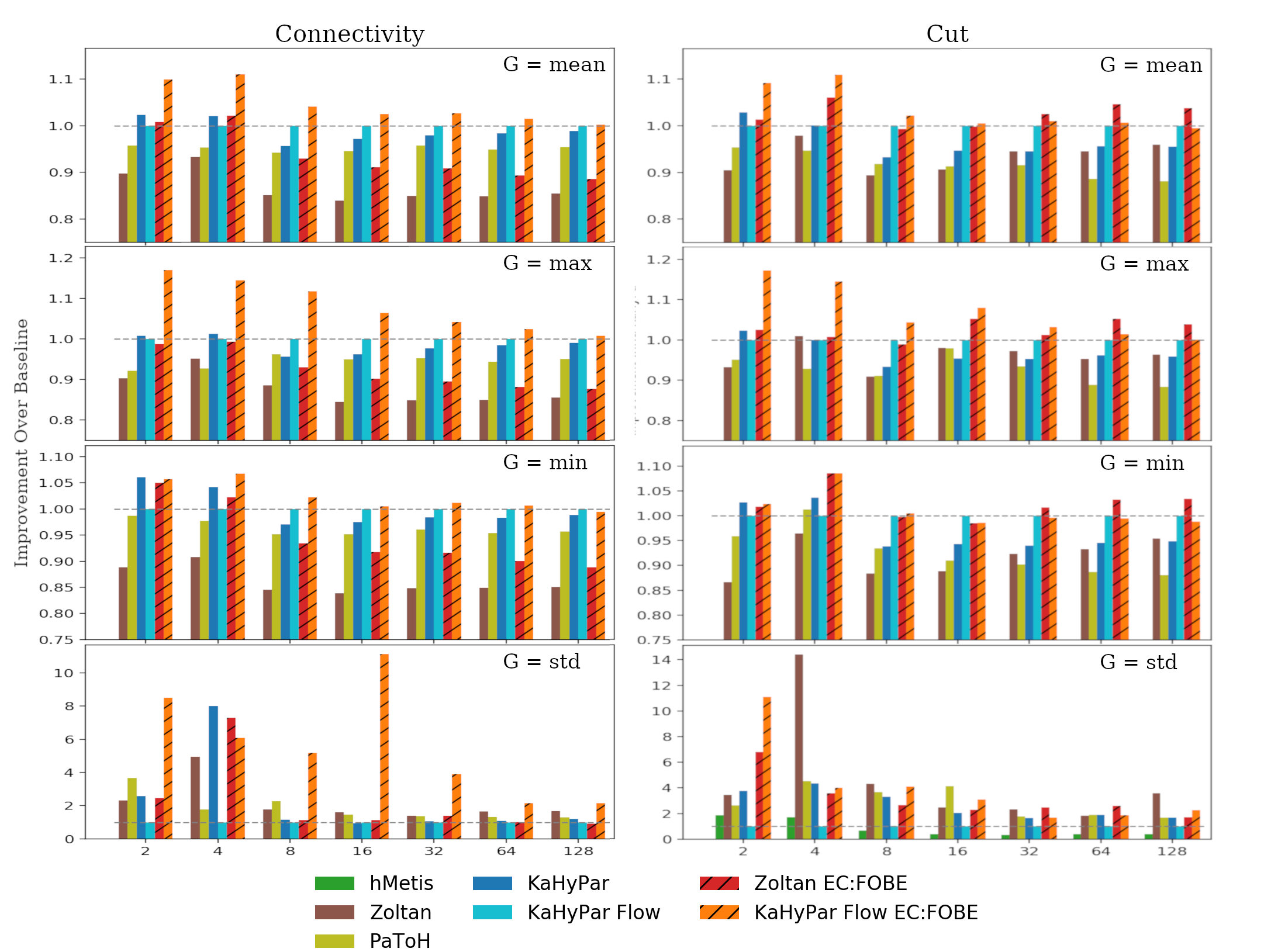
(a) The above depicts the relative performance of various partitioners, each using KaHyPar with flow-based refinement as a baseline. The results correspond to macro-summaries $\mathcal{I}$ (Eq. 8), where a value of 1, indicated by the horizontal dashed line, is baseline performance of $P_{B}$. We explore different summary statistics $G$, including mean, max, min, and standard deviation.

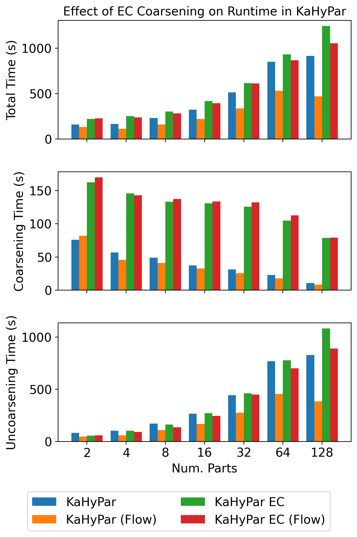
(b) Average Runtime of KaHyPar Across Benchmark.

Figure 3: Effect of Quality and Runtime

Runtime Our proposed coarsening introduces two sources of overhead into the typical partitioning process, as described in Section 4. We compare this runtime effect across our benchmark by focusing on KaHyPar. In Figure 3(b) we present average runtimes for each implementation, as well as isolated runtimes for the coarsening and uncoarsening phases. Note that when reporting runtime results for the embedding-based implementations of KaHyPar, these performance numbers represent an average across all considered embeddings. We find that embedding-based coarsening multiplies the time needed to coarsen an input hypergraph, which is due to the additional node-wise comparisons and sorting overhead. However, we also find that coarsening amounts to only a fraction of the overall petitioner runtime, which is dominated by the runtime of the uncoarsening phase, which is relatively unchanged.

We plot runtime distributions for FOBE and HOBE, across the benchmark in the supplemental information. These methods are slower and less easily distributed than the other considered embeddings. We find that the median considered FOBE embedding requires 1832 seconds, while the median HOBE embedding requires 8682 seconds. However, we note that runtime improvements of graph embeddings are an active field of research. Additionally, these runtimes are sensitive to optimizations, hardware, and hyperparameters. Our graph embeddings add a large factor to the runtime of multilevel partitioning, which may disqualify our proposed algorithm from “high performance” scenarios, such as hypergraph partitioning to accelerate scientific computing workloads at runtime [21]. However, applications such as placing circuits on a chip [25], recommending documents [56], machine learning on hypergraphs [55], or deep learning on hypergraphs [16], could all significantly benefit from the slow but higher-quality partitioning brought by embedding-based coarsening.

5 Conclusion

We propose embedding-based coarsening, an approach that leverages global structural features present in a pretrained hypergraph embedding in order improve the solution quality of multilevel hypergraph partitioning. This approach prioritizes self-similar regions of the hypergraph by visiting nodes in a deterministic order based on the embedding properties of each node’s neighborhood. From there, embedding-based coarsening matches nodes by a score that combines a more traditional edge-wise inner-product with the dot product of node embeddings. We observe that the introduction of embedding-based features provides a “tie-breaking” mechanism that ultimately preserves global structural features at the coarsest level in the V-cycle. We implement our proposed coarsening strategy in both KaHyPar [40] and Zoltan [14].

We observe a significant increase in quality for small values of $k$ (from 2 to 16) gained from embedding-based coarsening. For higher values of $k$ we observe overall quality that returns to the state-of-the-art baseline. Furthermore, we find that embedding-based coarsening improves partitioning quality significantly across a range of scenarios in both the KaHyPar and Zoltan frameworks. Specifically, KaHyPar with flow-based refinement [22] and embedding-based coarsening, using either FOBE or HOBE [45] to produce node embedding, scores consistently higher on average than all considered baselines. Furthermore, we find that by replacing the random node visit order in many coarsening algorithms with a deterministic strategy that prioritizes self-similar node pairs, we both improve solution quality while drastically reducing solution variance, often by an order of magnitude. Large scale results for all benchmarks and considered metrics is also available in the online appendix: sybrandt.com/2019/partition.

6 Acknowledgements

This work was supported by NSF awards MRI #1725573, DMS #1522751, and NRT #1633608. We would like to thank Sebastian Schlag from the Karlsruhe Institute of Technology for helping us to understand KaHyPar. We would also like to thank our editor and reviewers.

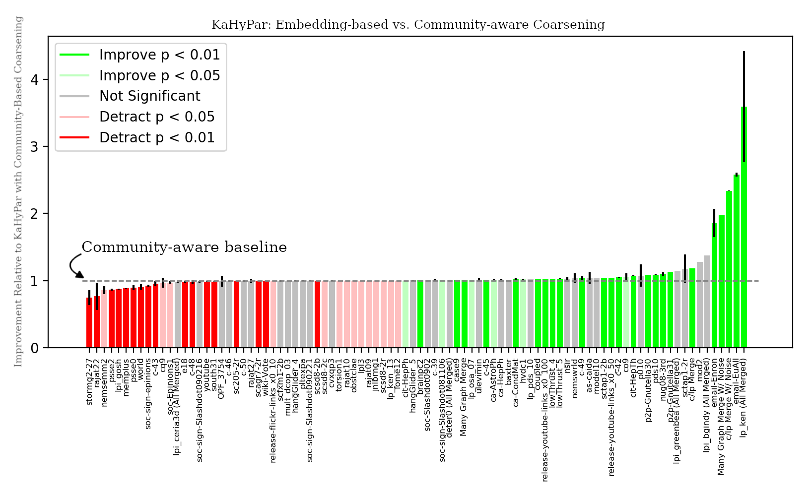
Figure 4: The above depicts per-hypergraph summary statistics, $I$ from Eq. 7, comparing KaHyPar with embedding-based coarsening ($P$) to KaHyPar with community-based coarsening ($P_{B}$). We use the mean over trails as our summary statistic $G$, as denoted by the height of each bar. A value higher than 1, which is emphasized by the dashed line, indicates better solution quality. The small black bar at the top of each graph indicates the standard deviation of trials, and the color of each bar indicates the statistical significance, where a more saturated color indicates a lower $p$-value. Hypergraph names are supplied across the horizontal axis, and graphs are ordered by relative improvement.

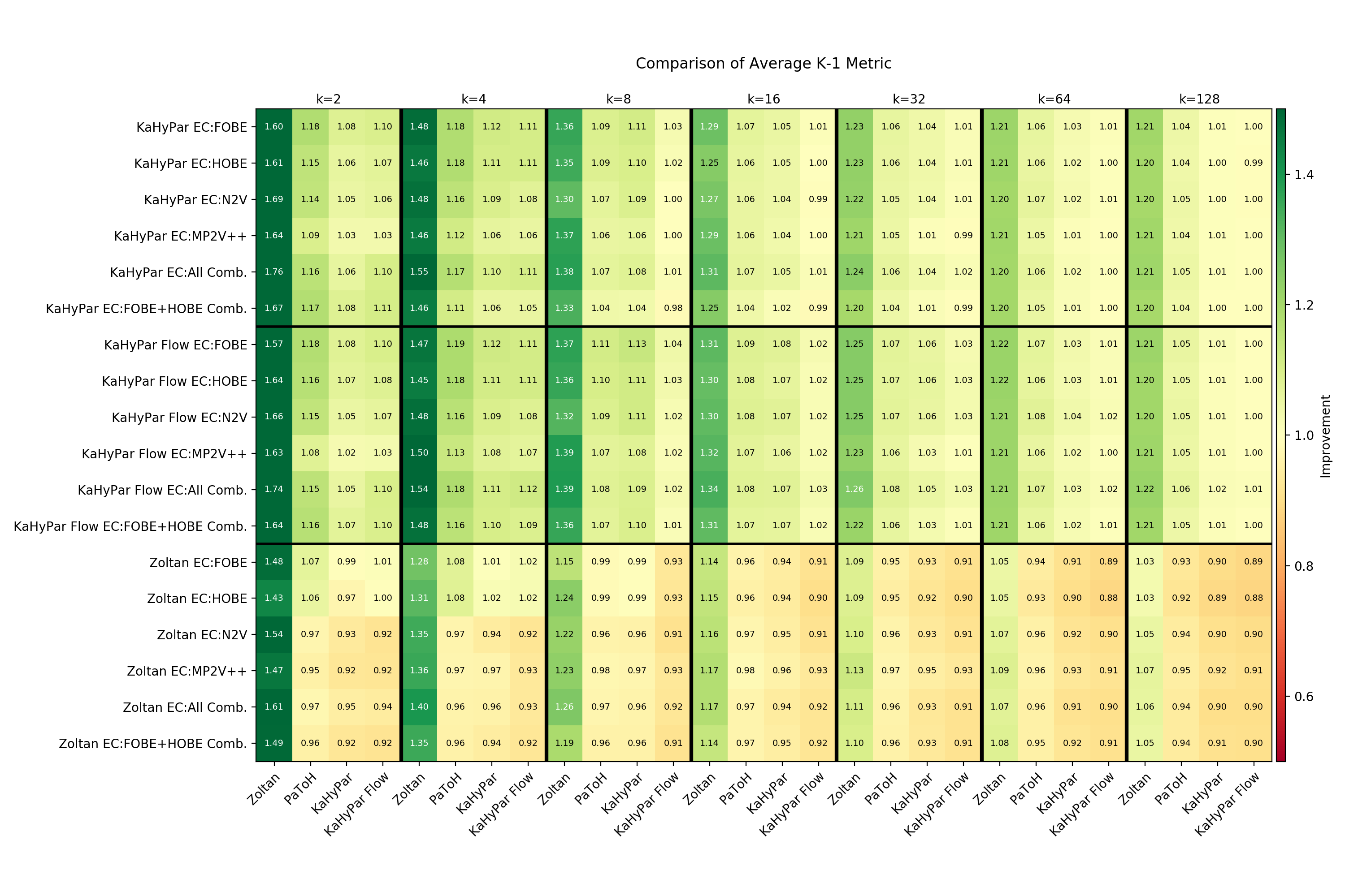
Figure 5: The above depicts the average improvement of the connectivity objective for all considered partitioners against all baselines. The values in each cell correspond to the macro-summary $\mathcal{I}$ using $G=\text{mean}$ to summarize trials. The online appendix includes similar tables for $G=\text{min, max, and std.}$

Table 2: Hypergraph Details.

$H$	$|V|$	$|E|$	$V$ Deg.		$E$ Size
			Mean	Std.	Mean	Std.
as-caida	26475	16538	3.657	29.016	5.855	29.016
baxter	30722	24255	3.528	5.359	4.469	5.359
brainpc2	27606	27606	6.498	131.257	6.498	131.257
c-39	9271	9271	14.757	41.233	14.757	41.233
c-42	10471	10471	10.532	41.339	10.532	41.339
c-43	11125	11125	11.117	72.602	11.117	72.602
c-45	13206	13206	13.210	85.104	13.210	85.104
c-46	14913	14913	8.744	42.022	8.744	42.022
c-48	18354	18354	9.049	16.866	9.049	16.866
c-49	21132	21132	7.431	14.452	7.431	14.452
c-50	22401	22401	8.644	22.902	8.644	22.902
c/lp Mixture W/ Noise	107776	69568	5.379	12.552	8.333	12.552
c/lp Mixture	107776	69368	5.374	12.552	8.350	12.552
ca-AstroPh	18479	17490	21.369	30.683	22.577	30.683
ca-CondMat	22523	20760	8.194	10.671	8.890	10.671
ca-HepPh	11670	10514	20.181	47.173	22.400	47.173
cari	1200	400	127.333	178.662	382.000	178.662
case9	14453	14453	10.238	105.257	10.238	105.257
cit-HepPh	28093	29526	14.913	27.227	14.189	27.227
cit-HepTh	22908	22610	15.294	43.314	15.496	43.314
co9	22829	10694	4.799	5.264	10.245	5.264
com-dblp-cmty	260998	13477	2.758	4.340	53.411	4.340
coupled	11341	11317	8.685	30.083	8.704	30.083
cq9	21503	9247	4.493	4.673	10.449	4.673
cvxqp3	17500	17500	6.998	3.626	6.998	3.626
deter0 Mixture	21872	7845	2.061	0.900	5.746	0.900
e18	38601	24617	4.053	5.472	6.356	5.472
email-Enron	35153	25481	10.140	33.809	13.989	33.809
email-EuAll	60532	33292	3.765	24.650	6.846	24.650
fome12	48920	24284	2.913	1.303	5.869	1.303
hangGlider_4	15561	15561	9.609	110.835	9.609	110.835
hangGlider_5	16011	16011	9.696	112.427	9.696	112.427
hvdc1	24842	24842	6.440	2.936	6.440	2.936
jnlbrng1	40000	40000	4.980	0.141	4.980	0.141
lowThrust_4	13562	13562	11.867	64.031	11.867	64.031
lowThrust_5	16262	16262	12.198	70.124	12.198	70.124
lp_ken Mixture	32418	19219	10.513	10.796	17.733	10.796
lp_ken_13	42659	23393	2.157	0.542	3.933	0.542
lp_osa_07	25067	1118	5.777	1.032	129.528	1.032
lp_pds_10	49932	16239	2.149	0.424	6.607	0.424
lpi_bgindy Mixture	97920	30322	11.824	9.319	38.182	9.319
lpi_ceria3d Mixture	39600	35384	11.891	23.733	13.308	23.733
lpi_gosh	13356	3662	7.474	5.231	27.260	5.231
lpi_greenbea Mixture	50319	24711	12.288	9.328	25.023	9.328
lpl3	33686	10655	2.979	0.184	9.418	0.184
Graph Mixture W/ Noise	110703	55507	3.650	2.971	7.279	2.971
Graph Mixture	110703	55307	3.645	2.970	7.296	2.970
memplus	17758	17758	7.104	22.035	7.104	22.035
mod2	65990	34355	3.022	2.883	5.804	2.883
model10	16819	4398	8.940	4.645	34.191	4.645
mult_dcop_01	25019	24817	7.710	144.682	7.773	144.682
mult_dcop_02	25019	24817	7.710	144.682	7.773	144.682
mult_dcop_03	25019	24817	7.708	144.682	7.771	144.682
nemsemm2	48857	6922	3.725	2.568	26.292	2.568
nemswrld	28496	6512	6.743	5.108	29.507	5.108
nsir	10055	4450	15.409	25.894	34.817	25.894
nug08-3rd	29856	19728	4.971	3.505	7.523	3.505
obstclae	39996	39996	4.941	0.418	4.941	0.418
OPF_3754	15435	15435	10.254	5.531	10.254	5.531
p010	19081	10071	6.183	4.984	11.715	4.984
p2p-Gnutella30	36345	9205	2.416	2.594	9.539	2.594
p2p-Gnutella31	62023	15383	2.368	2.669	9.549	2.669
pds10	16558	16558	9.038	7.258	9.038	7.258
pltexpa	70364	26894	2.033	1.288	5.319	1.288
psse0	11028	26694	9.286	6.075	3.836	6.075
psse2	11028	28632	10.452	6.713	4.026	6.713
rajat09	24482	24391	4.309	1.117	4.325	1.117
rajat10	30202	30101	4.311	1.116	4.326	1.116
rajat22	39801	38431	4.919	24.574	5.095	24.574
rajat27	20540	19163	4.786	16.261	5.130	16.261
release-flickr-links_x0_10	18612	18612	15.842	38.179	15.842	38.179
release-youtube-links_x0_100	115782	115778	3.999	7.222	3.999	7.222
release-youtube-links_x0_25	28945	28938	3.996	7.784	3.997	7.784
release-youtube-links_x0_50	57891	57888	3.999	7.222	3.999	7.222
sc205-2r	62422	35212	1.974	18.129	3.500	18.129
scagr7-2r	46679	32846	2.574	35.334	3.658	35.334
scfxm1-2b	33047	18266	3.337	6.509	6.038	6.509
scsd8-2b	35910	5130	3.140	17.607	21.982	17.607
scsd8-2c	35910	5130	3.140	17.607	21.982	17.607
scsd8-2r	60550	8650	3.141	22.885	21.990	22.885
sctap1-2b	33858	15390	2.937	17.447	6.462	17.447
sctap1-2r	63426	28830	2.938	23.857	6.464	23.857
soc-Epinions1	50328	31149	9.530	39.646	15.398	39.646
soc-Slashdot0811	77355	70893	11.622	37.228	12.682	37.228
soc-Slashdot0902	82159	71882	11.464	37.486	13.103	37.486
soc-sign-Slashdot081106	64371	27753	7.783	32.163	18.051	32.163
soc-sign-Slashdot090216	68836	30554	7.734	32.971	17.423	32.971
soc-sign-Slashdot090221	69038	30670	7.761	33.115	17.471	33.115
soc-sign-epinions	76359	42470	10.327	43.547	18.567	43.547
south31	35885	17989	3.120	132.364	6.224	132.364
stormg2-27	37485	14306	2.513	2.000	6.584	2.000
torsion1	39996	39996	4.941	0.418	4.941	0.418
ulevimin	46754	6394	3.515	2.714	25.703	2.714
wiki-Vote	2355	3728	43.018	40.735	27.175	40.735
world	66747	34106	2.974	2.751	5.820	2.751
youtube	90581	18173	3.107	8.121	15.487	8.121

References

- [1] Sameer Agarwal, Kristin Branson, and Serge Belongie. Higher order learning with graphs. In Proceedings of the 23rd international conference on Machine learning, pages 17–24. ACM, 2006.
- [2] Robin Andre, Sebastian Schlag, and Christian Schulz. Memetic multilevel hypergraph partitioning. In Proceedings of the Genetic and Evolutionary Computation Conference, GECCO ’18, pages 347–354, 2018.
- [3] Stephen T Barnard and Horst D Simon. Fast multilevel implementation of recursive spectral bisection for partitioning unstructured problems. Concurrency and computation: Practice and Experience, 6(2):101–117, 1994.
- [4] Charles-Edmond Bichot and Patrick Siarry. Graph partitioning. Wiley Online Library, 2011.
- [5] Erik G Boman, Umit V Catalyurek, Cédric Chevalier, Karen D Devine, Ilya Safro, and Michael M Wolf. Advances in parallel partitioning, load balancing and matrix ordering for scientific computing. In Journal of Physics: Conference Series, volume 180, pages 12008–12013. Institute of Physics Publishing, 2009.
- [6] A. Brandt and D. Ron. Chapter 1 : Multigrid solvers and multilevel optimization strategies. In J. Cong and J. R. Shinnerl, editors, Multilevel Optimization and VLSICAD. Kluwer, 2003.
- [7] Thang Nguyen Bui and Curt Jones. Finding good approximate vertex and edge partitions is np-hard. Information Processing Letters, 42(3):153–159, 1992.
- [8] Aydın Buluç, Henning Meyerhenke, Ilya Safro, Peter Sanders, and Christian Schulz. Recent advances in graph partitioning. In Algorithm Engineering: Selected Results and Surveys. LNCS 9220, Springer-Verlag, pages 117–158. Springer, 2016.
- [9] Shaosheng Cao, Wei Lu, and Qiongkai Xu. Deep neural networks for learning graph representations. In Thirtieth AAAI conference on artificial intelligence, 2016.
- [10] Ümit Çatalyürek and Cevdet Aykanat. Patoh (partitioning tool for hypergraphs). Encyclopedia of Parallel Computing, pages 1479–1487, 2011.
- [11] Umit V Catalyurek and Cevdet Aykanat. Hypergraph-partitioning-based decomposition for parallel sparse-matrix vector multiplication. IEEE Transactions on parallel and distributed systems, 10(7):673–693, 1999.
- [12] Jie Chen and Ilya Safro. Algebraic distance on graphs. SIAM Journal on Scientific Computing, 33(6):3468–3490, 2011.
- [13] Timothy A Davis and Yifan Hu. The university of florida sparse matrix collection. ACM Transactions on Mathematical Software (TOMS), 38(1):1, 2011.
- [14] Karen D Devine, Erik G Boman, Robert T Heaphy, Rob H Bisseling, and Umit V Catalyurek. Parallel hypergraph partitioning for scientific computing. In Parallel and Distributed Processing Symposium, 2006. IPDPS 2006. 20th International, pages 10–pp. IEEE, 2006.
- [15] Yuxiao Dong, Nitesh V Chawla, and Ananthram Swami. metapath2vec: Scalable representation learning for heterogeneous networks. In Proceedings of the 23rd ACM SIGKDD International Conference on Knowledge Discovery and Data Mining, pages 135–144. ACM, 2017.
- [16] Yifan Feng, Haoxuan You, Zizhao Zhang, Rongrong Ji, and Yue Gao. Hypergraph neural networks. In Proceedings of the AAAI Conference on Artificial Intelligence, volume 33, pages 3558–3565, 2019.
- [17] Charles M Fiduccia and Robert M Mattheyses. A linear-time heuristic for improving network partitions. In Papers on Twenty-five years of electronic design automation, pages 241–247. ACM, 1988.
- [18] Ming Gao, Leihui Chen, Xiangnan He, and Aoying Zhou. BiNE: Bipartite Network Embedding. In The 41st International ACM SIGIR Conference on Research & Development in Information Retrieval, SIGIR ’18, pages 715–724, New York, NY, USA, 2018. ACM.
- [19] Aditya Grover and Jure Leskovec. node2vec: Scalable feature learning for networks. In Proceedings of the 22nd ACM SIGKDD international conference on Knowledge discovery and data mining, pages 855–864. ACM, 2016.
- [20] Matthias Hein, Simon Setzer, Leonardo Jost, and Syama Sundar Rangapuram. The total variation on hypergraphs-learning on hypergraphs revisited. In Advances in Neural Information Processing Systems, pages 2427–2435, 2013.
- [21] Bruce Hendrickson and Alex Pothen. Combinatorial scientific computing: The enabling power of discrete algorithms in computational science. In International Conference on High Performance Computing for Computational Science, pages 260–280. Springer, 2006.
- [22] Tobias Heuer, Peter Sanders, and Sebastian Schlag. Network Flow-Based Refinement for Multilevel Hypergraph Partitioning. In 17th International Symposium on Experimental Algorithms (SEA 2018), pages 1:1–1:19, 2018.
- [23] Tobias Heuer and Sebastian Schlag. Improving coarsening schemes for hypergraph partitioning by exploiting community structure. In 16th International Symposium on Experimental Algorithms, (SEA 2017), pages 21:1–21:19, 2017.
- [24] George Karypis. hmetis 1.5: A hypergraph partitioning package. http://www. cs. umn. edu/~ metis, 1998.
- [25] George Karypis, Rajat Aggarwal, Vipin Kumar, and Shashi Shekhar. Multilevel hypergraph partitioning: applications in vlsi domain. IEEE Transactions on Very Large Scale Integration (VLSI) Systems, 7(1):69–79, 1999.
- [26] George Karypis and Vipin Kumar. A fast and high quality multilevel scheme for partitioning irregular graphs. SIAM J. Sci. Comput., 20(1):359–392, 1998.
- [27] Brian W Kernighan and Shen Lin. An efficient heuristic procedure for partitioning graphs. Bell Syst. Tech. J., 49(2):291–307, 1970.
- [28] Thomas N Kipf and Max Welling. Semi-supervised classification with graph convolutional networks. arXiv preprint arXiv:1609.02907, 2016.
- [29] Thomas Lengauer. Combinatorial algorithms for integrated circuit layout. Springer Science & Business Media, 2012.
- [30] Adam Lerer, Ledell Wu, Jiajun Shen, Timothee Lacroix, Luca Wehrstedt, Abhijit Bose, and Alex Peysakhovich. PyTorch-BigGraph: A Large-scale Graph Embedding System. In Proceedings of the 2nd SysML Conference, Palo Alto, CA, USA, 2019.
- [31] Tomas Mikolov, Ilya Sutskever, Kai Chen, Greg S Corrado, and Jeff Dean. Distributed representations of words and phrases and their compositionality. In Advances in neural information processing systems, pages 3111–3119, 2013.
- [32] Mark Newman. Networks: an introduction. Oxford university press, 2010.
- [33] Bryan Perozzi, Rami Al-Rfou, and Steven Skiena. Deepwalk: Online learning of social representations. In Proceedings of the 20th ACM SIGKDD international conference on Knowledge discovery and data mining, pages 701–710. ACM, 2014.
- [34] Benjamin Recht, Christopher Re, Stephen Wright, and Feng Niu. Hogwild: A lock-free approach to parallelizing stochastic gradient descent. In Advances in neural information processing systems, pages 693–701, 2011.
- [35] Dorit Ron, Ilya Safro, and Achi Brandt. Relaxation-based coarsening and multiscale graph organization. Multiscale Modeling & Simulation, 9(1):407–423, 2011.
- [36] Ehsan Sadrfaridpour, Talayeh Razzaghi, and Ilya Safro. Engineering fast multilevel support vector machines. Machine Learning, 108(11):1879–1917, 2019.
- [37] Ilya Safro, Dorit Ron, and Achi Brandt. Multilevel algorithms for linear ordering problems. Journal of Experimental Algorithmics (JEA), 13:4, 2009.
- [38] Ilya Safro, Peter Sanders, and Christian Schulz. Advanced coarsening schemes for graph partitioning. ACM Journal of Experimental Algorithmics (JEA), 19:2–2, 2015.
- [39] Peter Sanders and Christian Schulz. Engineering multilevel graph partitioning algorithms. In European Symposium on Algorithms, pages 469–480. Springer, 2011.
- [40] Sebastian Schlag, Vitali Henne, Tobias Heuer, Henning Meyerhenke, Peter Sanders, and Christian Schulz. k-way hypergraph partitioning via n-level recursive bisection. In 18th Workshop on Algorithm Engineering and Experiments, (ALENEX 2016), pages 53–67, 2016.
- [41] Ruslan Shaydulin, Jie Chen, and Ilya Safro. Relaxation-based coarsening for multilevel hypergraph partitioning. Multiscale Modeling & Simulation, 17(1):482–506, 2019.
- [42] Ruslan Shaydulin and Ilya Safro. Aggregative coarsening for multilevel hypergraph partitioning. 17th International Symposium on Experimental Algorithms (SEA 2018), 2018.
- [43] Michael A Shepherd, Carolyn R Watters, and Yao Cai. Transient hypergraphs for citation networks. Information Processing & Management, 26(3):395–412, 1990.
- [44] L.E. Stock. Strategic Logistics Management. Cram101 Textbook Outlines. Lightning Source Inc, 2006.
- [45] Justin Sybrandt and Ilya Safro. First-and High-Order Bipartite Embeddings. submitted, arXiv preprint arXiv:1905.10953, 2019.
- [46] Jian Tang, Meng Qu, Mingzhe Wang, Ming Zhang, Jun Yan, and Qiaozhu Mei. Line: Large-scale information network embedding. In Proceedings of the 24th International Conference on World Wide Web, pages 1067–1077. International World Wide Web Conferences Steering Committee, 2015.
- [47] Lei Tang, Huan Liu, Jianping Zhang, and Zohreh Nazeri. Community evolution in dynamic multi-mode networks. In Proceedings of the 14th ACM SIGKDD international conference on Knowledge discovery and data mining, pages 677–685. ACM, 2008.
- [48] Aleksandar Trifunovic. Parallel algorithms for hypergraph partitioning. PhD thesis, University of London, 2006.
- [49] Aleksandar Trifunović and William J Knottenbelt. Parallel multilevel algorithms for hypergraph partitioning. Journal of Parallel and Distributed Computing, 68(5):563–581, 2008.
- [50] Anton Tsitsulin, Davide Mottin, Panagiotis Karras, and Emmanuel Müller. Verse: Versatile graph embeddings from similarity measures. In Proceedings of the 2018 World Wide Web Conference, pages 539–548, 2018.
- [51] Brendan Vastenhouw and Rob H Bisseling. A two-dimensional data distribution method for parallel sparse matrix-vector multiplication. SIAM review, 47(1):67–95, 2005.
- [52] Daixin Wang, Peng Cui, and Wenwu Zhu. Structural deep network embedding. In Proceedings of the 22nd ACM SIGKDD international conference on Knowledge discovery and data mining, pages 1225–1234, 2016.
- [53] Chenzi Zhang, Shuguang Hu, Zhihao Gavin Tang, and TH Chan. Re-revisiting learning on hypergraphs: confidence interval and subgradient method. In Proceedings of the 34th International Conference on Machine Learning-Volume 70, pages 4026–4034. JMLR. org, 2017.
- [54] Zi-Ke Zhang and Chuang Liu. A hypergraph model of social tagging networks. Journal of Statistical Mechanics: Theory and Experiment, 2010(10):P10005, 2010.
- [55] Dengyong Zhou, Jiayuan Huang, and Bernhard Schölkopf. Learning with hypergraphs: Clustering, classification, and embedding. In Advances in neural information processing systems, pages 1601–1608, 2007.
- [56] Yu Zhu, Ziyu Guan, Shulong Tan, Haifeng Liu, Deng Cai, and Xiaofei He. Heterogeneous hypergraph embedding for document recommendation. Neurocomputing, 216:150–162, 2016.