Climate Policy under Spatial Heat Transport: Cooperative and Noncooperative Regional Outcomes

Abstract

We build a novel stochastic dynamic regional integrated assessment model (IAM) of the climate and economic system including a number of important climate science elements that are missing in most IAMs. These elements are spatial heat transport from the Equator to the Poles, sea level rise, permafrost thaw and tipping points. We study optimal policies under cooperation and noncooperation between two regions (the North and the Tropic-South) in the face of risks and recursive utility. We introduce a new general computational algorithm to find feedback Nash equilibrium. Our results suggest that when the elements of climate science are ignored, important policy variables such as the optimal regional carbon tax and adaptation could be seriously biased. We also find the regional carbon tax is significantly smaller in the feedback Nash equilibrium than in the social planner’s problem in each region, and the North has higher carbon taxes than the Tropic-South.

Keywords: Integrated Assessment Model, spatial heat transport, carbon taxes, adaptation, sea level rise, stochastic tipping points, Epstein-Zin preferences, feedback Nash equilibrium

JEL Classification: Q54, Q58, C61, C63, C68, C73

1 Introduction

A major characteristic of leading integrated assessment models (IAMs) such as RICE-2010 (Nordhaus, 2010) or DICE-2016 (Nordhaus, 2017) is that the geophysical sector of the model determines the mean surface temperature through the carbon cycle, which in turn determines the damage function. Thus damages are related to the mean surface temperature of the planet.

A well-established fact in the science of climate change, however, is that when the climate cools or warms, high latitude regions tend to exaggerate the changes seen at lower latitudes (e.g., Langen and Alexeev, 2007; IPCC, 2013). This effect is called polar amplification (PA) and indicates that, under global warming, the temperature at the latitudes closer to the Poles will increase faster than at latitudes nearer to the Equator. PA is especially strong in the Arctic and is sometimes called “Arctic amplification”. For example, Bekryaev et al. (2010) document a high-latitude (greater than 60 °N) warming rate of 1.36 degrees centigrade per century from 1875 to 2008. This trend is almost twice that of the Northern Hemisphere trend of 0.79 degrees centigrade per century.

Spatial heat and moisture transport, and the resulting PA, suggest that a better representation of the climate science underlying IAMs would be a geophysical sector structure which accounts for these phenomena. This implies that, in the IAM output, the surface temperature anomaly will be differentiated across spatial zones of the globe. The spatial temperature differentiation is important for the economics of climate change because it provides the impact of PA on the structure of the economic damages. PA will accelerate the loss of Arctic sea ice, which in turn has consequences for melting land ice that is associated with a potential meltdown of the Greenland and West Antarctica ice sheets which could cause serious global sea level rise (SLR).

Another source of damage associated with PA relates to the thawing of the permafrost, which is expected to bring about widespread changes in ecosystems and damage to infrastructure, along with release of greenhouse gases (GHGs) which exist in permafrost carbon stocks (see, e.g., IPCC, 2013; Schuur et al., 2015). Furthermore, recent studies suggest that Arctic amplification might increase the frequency of extreme weather events (Cohen et al., 2018), although this remains a controversial issue (Overland and Wang, 2018).

The well-known “burning embers” diagram in Lenton and Schellnhuber (2007) shows the ranking of tipping elements by order of proximity to the present time. The “nearest” three potential tipping points are located in the high latitudes of the Northern Hemisphere (Arctic summer sea ice loss, Greenland ice sheet melt and boreal forest loss). Because of PA in the Arctic, each degree increase in planetary yearly mean temperature leads to approximately two degrees increase in the Arctic latitudes. Thus natural phenomena occurring in high latitudes, due to spatial heat and moisture transport, can cause economic damages in lower latitudes. These spatial impacts, which could have important implications for climate change policies, are not embodied in the current generation of IAMs. The RICE model (Nordhaus, 2010) – the regional version of DICE (Nordhaus, 2017) – still treats the climate system by using the globally averaged measure of temperature and neglects heat and moisture transport and especially PA.

Hassler and Krusell (2012) extend Golosov et al. (2014) to multi-regions. While their work is elegant, as is that of Golosov et al. (2014), they do not deal with poleward heat transport, multi-layer carbon cycles, separation of atmospheric and oceanic layers, and regional tipping points, as we do here. van der Ploeg and de Zeeuw (2016) and Jaakkola and van der Ploeg (2018) develop interesting two-region models with tipping points that deal explicitly with non-cooperative and cooperative institutional structures. But they do not include geographic specification of regions, poleward heat transport, recursive preferences, or the more realistic multi-layer modeling of the carbon cycle and the temperature response to anthropogenic forcing as we have. Thus neither they nor Golosov et al. (2014) and Hassler and Krusell (2012) are able to study the effects of different values of the intertemporal elasticity of substitution (IES) and risk aversion parameters, or the effects of neglecting poleward heat transport on regional carbon taxes, as we are able to do with our richer and more realistic modeling of the interaction between climate dynamics and economic dynamics.

Another very recent IAM model of Krusell and Smith (2017) deals with space at a much finer scale than the present paper and contrasts market structures, including autarky and full borrowing and lending. However, their model does not address issues related to heat and moisture transport, SLR, permafrost thaw and the impacts of tipping points, as we do here. Thus we feel that our work is complementary to that of Krusell and Smith (2017) and not competitive. As mentioned above, one novel contribution of the present paper is to develop an IAM which incorporates spatial impacts associated with heat and moisture transport, along with treatment of uncertainty and tipping points. As far as we know, no other IAM treats these issues as we do here.

The stochastic IAM developed in this paper is a complex two-regional model with a more realistic – relative to existing models – geophysical sector and its solution requires the use of advanced numerical methods. Thus we adapt computational methods related to the DSICE model of Cai et al. (forthcoming). The DSICE framework is a stochastic generalization of DICE, which does not take into account the heat and moisture transport dynamics of the climate system. We adapt DSICE by disaggregating the globe into regions. However, DSICE is only a social planner’s model and its computational method is for solving social planner’s problems. Besides a social planner’s model, we also study feedback Nash equilibrium in this paper, and we develop a new general computational method to solve the high-dimensional dynamic stochastic game (with ten continuous state variables and one discrete state variable) with recursive utility.

Most IAMs are based on a social planner’s problem assuming that all countries are cooperative and the social planner can allocate resources without border frictions, so they can just provide a polar solution as there are very few unselfish sovereigns in the real world. It would be interesting if we can find another polar solution under a noncooperative Nash equiloibrium. To our best knowledge, van der Ploeg and de Zeeuw (2016) and Jaakkola and van der Ploeg (2018) are the only work in finding optimal climate policy under noncooperation. However, van der Ploeg and de Zeeuw (2016) just solve an open-loop Nash equilibrium whose optimal decisions depend on time and the initial state only; Jaakkola and van der Ploeg (2018) solve a symmetric feedback Nash equilibrium (FBNE) under a low-dimensional continuous-time model using the Hamilton-Jacobi-Bellman equation method, but in most cases FBNE is not symmetric. This paper is the first to numerically find optimal climate policy under both the social planner’s cooperative world and (asymmetrical) FBNE under a realistic discrete-time dynamic stochastic model with more than ten continuous state variables.

We call our model a Dynamic Integration of Regional Economy and Spatial Climate under Uncertainty (DIRESCU). In developing DIRESCU, we follow the two-region approach of Langen and Alexeev (2007) but change their regions as follows: region 1 is the region north of latitude 30°N to 90°N (called the North), while region 2 is the region from latitude 90°S (the South Pole) to 30°N (called the Tropic-South). Heat and moisture transport take place northbound from the tropical belt of latitudes north of the Equator which are included in the Tropic-South toward the North.

The interaction of the geophysical sector of DIRESCU with the economic sector is reflected in the damage function. We introduce separate damage functions in each region and allow for damages in the Tropic-South to be caused by an increase in temperature (i.e., PA) in the North. For example, the increased amplification of the temperature anomaly in the high north latitudes increases the hazard rate of tipping events in the high north latitudes toward earlier arrival times. Hence any associated damages caused to lower latitudes by warming in the higher north latitudes, e.g., increased melting of land ice leading to SLR damages in the lower latitudes, will be increased by PA, even though the high northern latitudes may benefit from additional warming.

The rest of the economic module is based on a two-region differentiation of DICE-2016 (Nordhaus, 2017). We model the economic interactions between the regions with an adjustment cost function, and we allow for adaptation expenses in each region. Krusell and Smith (2017) compare the two market structures of complete autarky and full international borrowing and lending and find that the market structures do not have a large impact on their results. While we can study autarky as Krusell and Smith (2017) do by raising the cost of interaction to induce autarky, our formulation of economic interactions does not include the case of full borrowing and lending as in their model. We have ignored serious modeling of market structure in order to focus on some elements of geophysics that are ignored in other contributions, including that of Krusell and Smith (2017). We do this to provide new insights regarding the importance of spatial heat and moisture transport phenomena in climate change policy.

The present paper innovates relative to popular IAMs at the tractable level of complexity in the literature (e.g., Nordhaus’s DICE and RICE models, the even more complex DSICE model and many others) in a number of ways. In particular, (i) we incorporate an endogenous SLR module, an endogenous permafrost melt module and, especially, we add the more realistic geophysics of spatial heat and moisture transport from low latitudes to high latitudes, while keeping the three-layer carbon cycle of DICE and RICE, and expanding the two-layer temperature module of DICE and RICE to a three-layer module; (ii) We introduce recursive preferences and we consider a wide range of parameter values of risk aversion and IES; (iii) We allow for adaptation to regional damage from SLR and temperature increase; (iv) Our paper goes beyond the single-region DSICE model by developing a new general computational method to numerically solve a dynamic stochastic FBNE of two regions.

We calibrate our many parameter values to match history as well as to fit the representative concentration pathway (RCP) scenarios (Meinshausen et al., 2011b). The main results of this paper are summarized below.

First, stochastic processes of regional carbon taxes are derived and various uncertainty fan charts are presented and compared with and without heat and moisture transport as well as for a range of risk aversion and IESs, under cooperation and noncooperation between regions. Moreover, the North has much higher regional carbon taxes than the Tropic-South. Our figures and tables provide a much more thorough quantification of the multitude of types of uncertainties than the received regional IAM literature at the DICE/RICE level of complexity.

Second, the non-cooperative dynamic stochastic game between the regions leads to much lower regional carbon taxes than the social planner’s model with economic interactions between the regions. If the economy in each region is closed, then the social planner’s model has much larger regional carbon taxes and much larger surface temperature increases than in the case with economic interactions.

Third, neglecting heat and moisture transport as in RICE and other regional IAMs that do not account for this added geophysics leads to many biases, including inaccurate forecasting of the first time of arrival of potential tipping points located in the high latitudes of the Northern Hemisphere. The low (high) latitude regions would be hotter (colder) if poleward heat transport were absent, hence damages in the low latitude regions would be higher, since they are already under heat stress and transporting some of that heat poleward helps relieve this heat stress. For example, solutions without heat transport will underestimate what actual heat-related damage there is in the North, and overestimate the actual heat-related damage in the Tropic-South. Without heat transport, the adaptation rates in the North will be underestimated as its corresponding atmospheric temperature anomaly is underestimated, and the adaptation rates in the Tropic-South will be overestimated as its corresponding atmospheric temperature anomaly is overestimated.

Fourth, endogenous SLR and adaptation are important new contributions of our modeling. In this way we capture the projected increased diversion into adapting to SLR (e.g., spending resources on SLR-protective infrastructure). The projected earlier arrival of increased melting of land ice in the Northern Hemisphere high latitudes due to our inclusion of heat transport means a potential increase in SLR damages in coastal low latitude areas relative to the projections when heat transport is ignored. Ignoring SLR underestimates the regional carbon taxes significantly, and ignoring adaptation overestimates the regional carbon taxes significantly.

Fifth, the optimal regional carbon taxes for both regions tend to be larger for larger IES values for climate tipping risks, in a cooperative or non-cooperative world. This is consistent with empirical findings in finance that greater IESs in Epstein–Zin recursive preferences (Epstein and Zin, 1989) imply that long-term risk matters and carbon taxes are larger. This result is also consistent with the findings in the DSICE model Cai et al. (forthcoming).

The paper is organized as follows. Section 2 builds DIRESCU. We calibrate our spatial climate system and the economic system using DICE and RICE, as well as data from other literature such as IPCC (2013). Section 3 discusses the social planner’s problem and the regional feedback Nash equilibrium under climate tipping risk and Epstein–Zin preferences to address the smoothness of consumption across time and risk aversion. Section 4 introduces our new computational method to solve FBNE for a general dynamic game. Section 5 discusses the results of the DIRESCU model and Section 6 concludes.

2 Model Setup

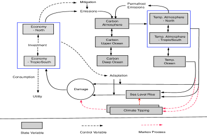
The deterministic version of our DIRESCU model follows DICE-2016 (Nordhaus, 2017), which maximizes social welfare with trade-offs between carbon dioxide (CO₂) abatement, consumption and investment. Our model has been augmented with an additional control, relative to DICE-2016, by including adaptation to climate change following de Bruin et al. (2009). DIRESCU has two regions: the first one (indexed with $i=1$) is the North from latitude 30°N to 90°N and the second one (indexed with $i=2$) is the Tropic-South from latitude 90°S to 30°N. We first model it as a social planner problem with both economic and climate interaction between two regions, SLR, permafrost thaw and climate tipping risks (in the deterministic model, the risks are ignored). We then change it to a dynamic stochastic game and solve its feedback Nash equilibrium. The big picture of the model setup is depicted in Figure 1 and its details are described below.

Figure 1: The DIRESCU model

2.1 The Climate System

The climate system contains four modules: the carbon cycle, the temperature system, SLR and permafrost thaw. In our calibration of the climate system, we use the four RCP scenarios (i.e., RCP2.6, RCP4.5, RCP6, and RCP8.5) (Meinshausen et al., 2011b) and DICE/RICE optimal scenarios (i.e., the optimal solutions of DICE-2016 and RICE-2010 with optimal mitigation policy), where we define each scenario as a combination of pathways of global emissions, atmospheric carbon concentration, global radiative forcing, and globally averaged surface temperature relative to 1900 levels. For the RCP scenarios, the pathways of atmospheric carbon concentration, global radiative forcing, and globally averaged surface temperature are generated from the software MAGICC (Meinshausen et al., 2011a), using the corresponding pathways of global emissions as the input to the software. The pathways of global emissions are provided by MAGICC too. Appendix A.2 shows that our calibrated system fits these scenarios, history, as well as other data in the literature such as regional temperature projections reported in IPCC (2013).

2.1.1 Carbon Cycle

We follow DICE-2016 in using three-layer carbon concentrations: atmospheric carbon, carbon in the upper ocean and carbon in the deep ocean. Let $\mathbf{M}_{t}=(M_{t}^{\mathrm{AT}},M_{t}^{\mathrm{UO}},M_{t}^{\mathrm{DO}})^{\top}$ represent the carbon concentration in the atmosphere, the upper ocean and the deep ocean. Then the three-layer carbon cycle system can be represented as:

$$\mbox{{M}}_{t+1}=\mathbf{\mathbf{\Phi}}_{\mathrm{M}}\mathbf{M}_{t}+\left(E_{t},0,0\right)^{\top},$$ (1)

where $E_{t}$ is global carbon emissions (billions of metric tons) and

$$\mathbf{\Phi}_{\mathrm{M}}=\left[\begin{array}[]{ccc}1-\phi_{12}&\phi_{21}\\ \phi_{12}&1-\phi_{21}-\phi_{32}&\phi_{32}\\ &\phi_{23}&1-\phi_{32}\end{array}\right].$$

The parameters $\phi_{ij}$ are calibrated against the four RCP scenarios and the DICE-2016 optimal scenario. For every scenario, we can use its pathway of emissions as the input $E_{t}$ to our carbon cycle system (1). Our carbon cycle provides as output a pathway of atmospheric carbon concentration for each scenario. We calibrate a unique set of values for $\phi_{ij}$ so that the pathways of atmospheric carbon concentration are close to the scenarios’ pathways of atmospheric carbon concentration, for all scenarios.

2.1.2 Temperature Subsystem

The global radiative forcing representing the impact of CO₂ concentrations on the surface temperature of the globe (watts per square meter from 1900) is

$$F_{t}=\eta\log_{2}\left(M_{t}^{\mathrm{AT}}/M_{*}^{\mathrm{AT}}\right)+F_{t}^{\mathrm{EX}},$$ (2)

where $\eta=3.68$ as in DICE-2016 and $F_{t}^{\mathrm{EX}}$ is the global exogenous radiative forcing.

We use $\mathbf{T}_{t}=(T_{t,1}^{\mathrm{AT}},T_{t,2}^{\mathrm{AT}},T_{t}^{\mathrm{OC}})^{\top}$ to represent the temperature anomaly (relative to 1900 levels) in the atmosphere (two regions) and the global ocean. Thus, the temperature system is

$$\mbox{{T}}_{t+1}=\mathbf{\Phi}_{\mathrm{T}}\mathbf{T}_{t}+\xi_{1}\left(F_{t},F_{t},0\right)^{\top},$$ (3)

where we assume that the global radiative forcing has the same effect on both regions, and

$$\mathbf{\Phi}_{\mathrm{T}}=\left[\begin{array}[]{ccc}1-\xi_{2}-\xi_{4}-\xi_{6}&\xi_{4}+\xi_{5}&\xi_{2}\\ \xi_{4}&1-\xi_{2}-\xi_{4}-\xi_{5}-\xi_{6}&\xi_{2}\\ \xi_{3}&\xi_{3}&1-2\xi_{3}\end{array}\right].$$

In transition equation (3) and transition matrix $\mathbf{\Phi}_{\mathrm{T}}$, the parameter $\xi_{1}$ is the temperature increase for each unit of radiative forcing, $\xi_{2}$ and $\xi_{3}$ represent transport between atmosphere and ocean, $\xi_{4}$ and $\xi_{5}$ are used to capture spatial heat and moisture transport, and $\xi_{6}$ represents the sensitivity of the outgoing long-wave radiation to atmospheric temperature changes.

Similarly to the calibration of the carbon cycle, we calibrate $\xi_{1},...,\xi_{6}$ against the RCP scenarios, the DICE-2016 optimal scenario, and the historical spatial temperatures in 1900-2015 from the Goddard Institute for Space Studies (GISTEMP Team, 2018). For each scenario, we use its pathway of radiative forcing as the input $F_{t}$ to our temperature system (3), which provides as output two regional pathways of atmospheric temperatures in the regions. Then we average the regional pathways to generate a globally averaged atmospheric temperature pathway. We calibrate a unique set of values for $\xi_{1},...,\xi_{6}$ so that the generated globally averaged atmospheric temperature pathways from our temperature system are close to the pathways of globally averaged atmospheric temperature for all scenarios and, at the same time, our regional temperatures in 2081-2100 are also close to the projected regional temperatures in 2081-2100 provided in IPCC (2013).

2.1.3 Sea Level Rise

Sea level rise is a serious problem caused by global warming. Table 4.1 of IPCC (2013) shows that, if the whole Greenland ice sheet melts, it will cause more than 7 meters (m) global mean SLR, and if the whole Antarctic ice sheet melts, it will lead to about 58 m global mean SLR. Moreover, once an ice sheet collapses, it is irreversible for millennia even if forcing is reversed (IPCC 2013, Table 12.4). Nerem et al. (2018) adduce evidence that SLR is accelerating from the historical data. Table 13.5 of IPCC (2013) shows SLR in 2100 ranging from about 0.44 m for RCP2.6 to about 0.74 m for RCP8.5. Figure 13.14 of IPCC (2013) shows that the likely range of SLR is from 1 to 3 m per degree Celsius of globally averaged surface temperature increase if the warming is sustained for millennia.

There are four main sources of SLR: thermal expansion, and melting of glaciers and ice cap, the Greenland ice sheet, and the Antarctic ice sheet. The west Antarctic ice sheet (WAIS) is vulnerable to ocean warming as most of it is below sea level and extensively exposed to the ocean. The contribution of a complete collapse of the marine WAIS is estimated at 3.3 m of SLR (Bamber et al., 2009). Thermal expansion is also due to ocean warming. The melting of glaciers and the Greenland ice sheet is due to atmospheric warming in the North. Therefore, we assume that the rate of SLR is dependent on north atmospheric temperature $T_{t,1}^{\mathrm{TA}}$ and ocean temperature $T_{t}^{\mathrm{OC}}$, and that a higher temperature implies a higher rate of SLR. We also assume that SLR, $S_{t}$, is irreversible. Thus, we let

$$S_{t+1}=S_{t}+\zeta_{1}^{\mathrm{SLR}}\left(T_{t,1}^{\mathrm{TA}}\right)^{\zeta_{2}^{\mathrm{SLR}}}+\zeta_{3}^{\mathrm{SLR}}T_{t}^{\mathrm{OC}},$$ (4)

where $\zeta_{1}^{\mathrm{SLR}}$, $\zeta_{2}^{\mathrm{SLR}}$ and $\zeta_{3}^{\mathrm{SLR}}$ are calibrated using the SLR data for four RCP scenarios in Table 13.5 of IPCC (2013) and Table 1 of Kopp et al. (2014).

2.1.4 Permafrost Thaw

With global warming, and in particular with PA, a large amount of CO₂ and CH₄ could be emitted from thawing permafrost in the Arctic and sub-Arctic regions, which contain about 1,700 GtC (gigaton of carbon) in permafrost soils, while about 1,035 GtC are stored in the surface permafrost (0-3 m depth) and could easily be emitted when they are thawed (Schuur et al., 2015). Schuur et al. (2015) show that an average carbon release from the permafrost zone by 2100 across models is about 92 GtC with a standard deviation of 17 GtC under RCP8.5. A higher atmospheric temperature in the North implies a higher emission rate. Thus, we assume that carbon emission from thawing permafrost is

$$E_{t}^{\mathrm{Perm}}=\zeta_{1}^{\mathrm{Perm}}\left(1-\frac{1}{1+\zeta_{2}^{\mathrm{Perm}}T_{t,1}^{\mathrm{AT}}+\zeta_{3}^{\mathrm{Perm}}\left(T_{t,1}^{\mathrm{AT}}\right)^{2}}\right).$$ (5)

Hope and Schaefer (2016) give a mean carbon emission path from thawing permafrost for the A1B scenario in IPCC (2007), so we use its annual time series to calibrate $\zeta_{1}^{\mathrm{Perm}}$, $\zeta_{2}^{\mathrm{Perm}}$ and $\zeta_{3}^{\mathrm{Perm}}$.

2.2 Climate Tipping Points

There are many uncertainties in the economic and climate system. For example, DSICE (Cai et al., forthcoming) discusses business cycle shocks in productivity and climate risks, and also deals with parameter uncertainty over the IES and risk aversion using uncertainty quantification. Lemoine and Traeger (2014) use a stylized model to study the impact of climate tipping points. Cai et al. (2016) use DSICE to study the impact of multiple interacting tipping points on the carbon tax policy. In this paper we introduce uncertainty regarding the emergence of endogenous tipping elements in the North into the spatial model with heat and moisture transport.

We assume that there is a representative tipping element that will take $D$ years to fully unfold its damage after it occurs. The final damage level is $\overline{J}$ as a fraction of output, and the tipping probability depends on the contemporaneous atmospheric temperature in the North. Let $J_{t}$ represent the damage level (as a fraction of output) of the tipping element, and let $\chi_{t}$ be the indicator representing whether the tipping event has happened or not before time $t$, so $\chi_{t}=0$ means that the tipping event has not happened, and $\chi_{t}=1$ means that it has happened before time $t$. Thus, the transition law of $J_{t}$ is

$$J_{t+1}=\min(\overline{J},\,J_{t}+\Delta)\chi_{t},$$ (6)

where $\Delta=\overline{J}/D$ is the annual increment of damage level after the tipping happens, and $\chi_{t}$ is a Markov chain with the probability transition matrix

$$\left[\begin{array}[]{cc}1-p_{t}&p_{t}\\ 0&1\end{array}\right],$$

where $p_{t}$ is the tipping probability from state $\chi_{t}=0$ to $\chi_{t}=1$. We let $p_{t}=1-\exp\left(-\varrho\max\left(0,T_{t,1}^{\mathrm{AT}}-1\right)\right),$where $\varrho$ is the hazard rate, so a higher atmospheric temperature in the North implies a higher tipping probability.

We use the Atlantic Meridional Overturning Circulation as the representative tipping element, and employ its default setup as in Cai et al. (2016), that is, $D=50$, $\overline{J}=0.15$ and $\varrho=0.00063$. To introduce a general model, we let

$$\chi_{t+1}=g(\chi_{t},\mathbf{T}_{t},\omega_{t})$$ (7)

denote the transition law for $\chi_{t}$.

2.3 The Economic System

We calibrate our regional economic system to match RICE projections over our regions. Appendix A.3 shows that our calibrated system fits RICE projections.

2.3.1 Production

The gross output at time $t$ in each region is determined by a Cobb-Douglas production function,

$$\mathcal{Y}_{t,i}\equiv A_{t,i}K_{t,i}^{\alpha}L_{t,i}^{1-\alpha},$$ (8)

with $\alpha=0.3$ and $L_{t,i}$ the exogenous population at time $t$ and region $i$ aggregated from RICE.

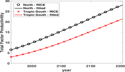
We use region-specific total factor productivity (TFP) $A_{t,i}$. Sachs (2001) stresses ecological specific technical progress and lists five reasons why TFPs in low latitude zones tend to be smaller than temperate latitude zones. Of course there are exceptions, as Sachs points out (e.g., Hong Kong and Singapore and, now, lower latitude parts of China and parallel parts of “Asian Tigers”). However, theory suggests that the economies that are “behind” should grow faster than the leaders because the leaders have already done the “heavy lifting” of the TFP R&D which the followers could presumably copy. For example, Sachs and McArthur (2002) discuss the transition from “adopter” to “innovator” for countries.

We let $A_{t,i}=A_{0,i}\exp\left(\alpha_{i}^{\mathrm{TFP}}\left(1-\exp\left(-d_{i}^{\mathrm{TFP}}t\right)\right)/d_{i}^{\mathrm{TFP}}\right),$ where $A_{0,i}$, $\alpha_{i}^{\mathrm{TFP}}$ and $d_{i}^{\mathrm{TFP}}$ are calibrated to match the TFP path in region $i$ which is computed from RICE by aggregating across the RICE subregions in region $i$.

2.3.2 Damages

In the deterministic case of DIRESCU, we consider two types of damages: damages to output from SLR and damages to output directly from temperature increase.

We follow RICE to let

$$D_{t,i}^{\mathrm{SLR}}=\pi_{1,i}S_{t}+\pi_{2,i}S_{t}^{2}$$ (9)

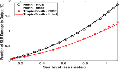
reflect the damage from SLR, $S_{t}$, as a fraction of output. We calibrate $\pi_{1,i}$ and $\pi_{2,i}$ to match the damage from SLR which is computed from RICE.

We follow DICE and RICE to assume a quadratic damage function for temperature increase

$$D_{t,i}^{\mathrm{T}}=\pi_{3,i}T_{t,i}^{\mathrm{AT}}+\pi_{4,i}(T_{t,i}^{\mathrm{AT}})^{2},$$ (10)

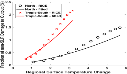
where $\pi_{3,i}$ and $\pi_{4,i}$ are calibrated to fit the aggregated projected damage from surface temperature change over RICE subregions.

With the quadratic damage function (10) for the Tropic-South, this region has damage of only 9% of its output if its regional surface temperature increase is the same as the global mean surface temperature in 2100 under RCP8.5, i.e., 4.7°C, as RICE does not take into account catastrophic damages. However, Burke et al. (2015) show that damages from high temperature increase in low- and mid-latitude regions are much higher, reducing projected global output by 23% in 2100 under RCP8.5, with the poorest 40% of countries (most being in our Tropic-South) having 75% reduction relative to a world without climate change. Dell et al. (2012) show that there are large and negative effects of higher temperatures on growth in poor countries, with about 1.3% economic growth reduction for a 1°C increase. Burke et al. (2015) show that climate change may lead to negative economic growth for some countries. Our estimate of damages follows DICE and RICE, that is, damages are proportional to instantaneous output, not to growth of TFP, so they may be underestimated for the Tropic-South and overestimated for the North. However, our estimate of damages to the high-latitude regions may also be underestimated, as we ignored potential damages from inequality between the regions (Hsiang et al., 2017).

2.3.3 Emissions, Adaptation, and Mitigation

Global carbon emissions at time $t$ are defined as

$$E_{t}\equiv\sum_{i=1}^{2}E_{t,i}^{\mathrm{Ind}}+E_{t}^{\mathrm{Perm}}+E_{t}^{\mathrm{Land}},$$

where $E_{t}^{\mathrm{Land}}$ is exogenous global carbon emissions from biological processes, $E_{t}^{\mathrm{Perm}}$ is emissions from permafrost thawing estimated by equation (5), and $E_{t,i}^{\mathrm{Ind}}=\sigma_{t,i}(1-\mu_{t,i})\mathcal{Y}_{t,i}$ is industrial emissions, where $\mu_{t,i}$ is an emission control rate and $\sigma_{t,i}$ is the carbon intensity in region $i$. We let

$$\sigma_{t,i}=\sigma_{0,i}\exp\left(-\alpha_{i}^{\sigma}\left(1-\exp\left(-d_{i}^{\sigma}t\right)\right)/d_{i}^{\sigma}\right),$$ (11)

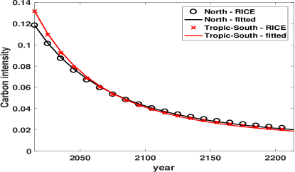
where $\sigma_{0,i}$, $\alpha_{i}^{\sigma}$ and $d_{i}^{\sigma}$ are calibrated to match the carbon intensity paths in region $i$ which are computed from RICE by aggregating across the RICE subregions in region $i$.

We include an adaptation choice variable $P_{t,i}$ for each region in our model as in de Bruin et al. (2009). Adaptation reduces damages to output from SLR and temperature increase. The output net of all damages including SLR, temperature anomaly and tipping becomes

$$Y_{t,i}\equiv(1-J_{t})\Omega_{t,i}\mathcal{Y}_{t,i}\equiv\frac{(1-J_{t})\mathcal{Y}_{t,i}}{1+(1-P_{t,i})(D_{t,i}^{\mathrm{SLR}}+D_{t,i}^{\mathrm{T}})}.$$ (12)

where $P_{t,i}\in[0,1]$ is the adaptation rate, and $\Omega_{t,i}$ is the damage factor after adaptation. We follow de Bruin et al. (2009) to assume that adaptation expenditure is $\Upsilon_{t,i}\equiv\eta_{1}P_{t,i}^{\eta_{2}}Y_{t,i},$ with $\eta_{1}=0.115$ and $\eta_{2}=3.6$.

We follow DICE to assume that mitigation expenditure is $\Psi_{t,i}\equiv\theta_{1,t,i}\mu_{t,i}^{\theta_{2}}Y_{t,i},$ where $\theta_{1,t,i}$ is the abatement cost as a fraction of output in region $i$ at time $t$. We use the DICE/RICE form to define $\theta_{1,t,i}=b_{0,i}\exp\left(-\alpha_{i}^{b}t\right)\sigma_{t,i}/\theta_{2},$ where $\alpha_{i}^{b}$ and $\theta_{2}$ are parameters given by RICE, and $b_{0,i}$ is the initial backstop price in region $i$.

Let $\widehat{Y}_{t,i}$ denote the output net of climate damage, mitigation expenditure and adaptation cost, that is, $\widehat{Y}_{t,i}=Y_{t,i}-\Psi_{t,i}-\Upsilon_{t,i}.$

2.3.4 Economic Interactions between Regions

In the economic system, each region’s stock of capital is the state variable $K_{t,i}$. Its law of motion is:

$$K_{t+1,i}=(1-\delta)K_{t,i}+I_{t,i},$$ (13)

where $\delta=0.1$ is the depreciation rate and $I_{t,i}$ is investment in region $i$. We model the economic interactions between two regions with the following adjustment cost function:

$$\Gamma_{t,i}\equiv\frac{B}{2}\widehat{Y}_{t,i}\left(\frac{I_{t,i}+c_{t,i}L_{t,i}}{\widehat{Y}_{t,i}}-1\right)^{2},$$ (14)

where $B$ is the intensity of the friction, and $c_{t,i}$ is per capita consumption in region $i$. The open economy situation corresponds to $B=0$, while a large $B$ approximates the closed economy with $\widehat{Y}_{t,i}=I_{t,i}+c_{t,i}L_{t,i}$ (note that $\Gamma_{t,i}=0$ could be caused by either the open economy or the closed economy, so we use $B=0$ and large $B$ to distinguish the two cases). Anderson and van Wincoop (2003) discuss border barriers and how costly they are. Similar adjustment cost functions have been used in Goulder et al. (2016). The economic interaction cost also includes the cost of avoiding carbon leakage between two regions. Eaton and Kortum (2002) find that if all countries (in their data set) collectively remove tariffs, then most countries will gain around 1% of output with mobile labor, and less than 0.5% with immobile labor. Since we assume mobile labor within each region but immobile between two regions, we estimate the economic interaction cost to be roughly 0.5% of output for each region and use this to calibrate $B$.

The market clearing condition with adjustment costs becomes

$$\sum_{i=1}^{2}\left(I_{t,i}+c_{t,i}L_{t,i}+\Gamma_{t,i}\right)=\sum_{i=1}^{2}\widehat{Y}_{t,i}.$$ (15)

3 Social Planner versus Nash Equilibrium

We use the Epstein–Zin preference (Epstein and Zin, 1989) to isolate the IES and risk aversion for our stochastic models under cooperation (a social planner’s model) or noncooperation (a dynamic stochastic game) between the regions.

3.1 Social Planner’s Model

With time separable utilities, a social planner maximizes the sum of discounted expected regional utilities subject to economic and climatic constraints for time separable utilities. Using the recursive utility, we use a transformation similar to that in Cai et al. (forthcoming) and then solve the Bellman equation:

$$V_{t}^{\mathrm{SP}}(\mathbf{x}_{t})=\max_{\mathbf{a}_{t}}\left\{\sum_{i=1}^{2}u(c_{t,i})L_{t,i}+\frac{\beta}{1-\frac{1}{\psi}}\left[\mathbb{E}_{t}\left(\left(\left(1-\frac{1}{\psi}\right)V_{t+1}^{\mathrm{SP}}(\mathbf{x}_{t+1})\right)^{\varTheta}\right)\right]^{1/\varTheta}\right\},$$ (16)

subject to (1), (3)-(4), (6)-(7), (12)-(13), and (15), where

$$\mathbf{x}_{t}=(K_{t,1},K_{t,2},M_{t}^{\mathrm{AT}},M_{t}^{\mathrm{UO}},M_{t}^{\mathrm{DO}},T_{t,1}^{\mathrm{AT}},T_{t,2}^{\mathrm{AT}},T_{t}^{\mathrm{OC}},S_{t},J_{t},\chi_{t})$$ (17)

is the vector of eleven state variables (the first ten variables are continuous), $\mathbf{a}_{t}=\left(I_{t,1},I_{t,2},c_{t,1},c_{t,2},\mu_{t,1},\mu_{t,2},P_{t,1},P_{t,2}\right)$ is the vector of decision variables (all are continuous), $\mathbb{E}_{t}$ is the expectation operator conditional on the time-$t$ information, $\beta$ is the discount factor, $u$ is a per capita utility function: $u(c)=c^{(1-1/\psi)}/(1-1/\psi),$with $\psi$ the IES, and $\varTheta=(1-\gamma)/(1-1/\psi)$ with $\gamma$ the risk aversion parameter. If $\psi\gamma=1$, then the recursive utility becomes time separable, and (16) becomes a standard Bellman equation. We use annual time steps, where the initial year ($t=0$) is 2015, and the terminal time ($t=T=300$) is the year 2315. The terminal value function $V_{T}^{\mathrm{SP}}(\mathbf{x}_{T})$ is computed as shown in Appendix A.7. We use $\psi=1.5$ and $\gamma=3.066$ as in Pindyck and Wang (2013) for our benchmark stochastic case. We use the parallel dynamic programming method (Cai et al., 2015) with simplicial complete Chebyshev polynomial approximation (Cai et al., 2018a) and time-varying approximation domains (Cai, forthcoming) on the Blue Waters supercomputer to solve the social planner’s problem. The computational method has been applied successfully to solve DSICE (Cai et al., 2016, forthcoming).

3.2 Feedback Nash Equilibrium

A non-cooperative world can be described as a situation in which each region acts a separate social planner and chooses emissions paths to maximize its own welfare subject to the relevant economic and climatic constraints and by taking emission of the other region as given. For this dynamic game two solution concepts are studied in the literature, the open loop Nash equilibrium and the feedback Nash equilibrium (FBNE). As is well known, the open loop Nash equilibrium does not possess the Markov perfect property and is not robust against unexpected changes in the state of the system. Therefore, the FBNE is considered to be a more satisfactory solution concept.

We derive the FBNE in a dynamic programming framework (e.g. Basar and Olsder 1999), so that the controls of each region depend on the states, and the solution is a Markov perfect non-cooperative regional equilibrium by construction. As shown in Appendix A.5 in our regional FBNE there is no transfer of capital between the regions, so the market clearing condition (15) is changed to

$$I_{t,i}+c_{t,i}L_{t,i} = \widehat{Y}_{t,i}$$ (18)

for $i=1,2$, and then adjustment costs $\Gamma_{t,i}$ are zero, so we can rewrite the transition laws of capital as

$$K_{t+1,i}=(1-\delta)K_{t,i}+\widehat{Y}_{t,i}-c_{t,i}L_{t,i}$$ (19)

after the substitution of $I_{t.i}$.

The FBNE is solved for a nonlinear dynamic stochastic programming problem, with recursive preferences, without symmetry, and regional feedback strategies which depend on a vector of eleven state variables (ten of which are continuous). We solve the following system of two Bellman equations:

$$V_{t,i}^{\mathrm{FBNE}}(\mathbf{x}_{t})=\max_{c_{t,i},P_{t,i},\mu_{t,i}}\left\{u(c_{t,i})L_{t,i}+\beta\mathcal{G}_{t,i}(\mathbf{x}_{t+1})\right\},$$ (20)

subject to

$$\mathbf{x}_{t+1}=\mathbf{f}_{t}(\mathbf{x}_{t},\mathbf{a}_{t}^{\mathrm{FBNE}},\omega_{t})$$ (21)

for $i=1,2$, where $\mathbf{x}_{t}$ is the vector of state variables defined in (17), $\mathbf{a}_{t}^{\mathrm{FBNE}}=\left(c_{t,1},c_{t,2},\mu_{t,1},\mu_{t,2},P_{t,1},P_{t,2}\right)$ is the vector of decision variables for the FBNE,

$$\mathcal{G}_{t,i}(\mathbf{x}_{t+1})\equiv\frac{1}{1-\frac{1}{\psi}}\left[\mathbb{E}_{t}\left(\left(\left(1-\frac{1}{\psi}\right)V_{t+1,i}^{\mathrm{FBNE}}(\mathbf{x}_{t+1})\right)^{\varTheta}\right)\right]^{1/\varTheta},$$ (22)

and $\mathbf{f}_{t}$ represents the vector of the transition laws of state variables: (1), (3), (4), (6), (7), and (19) for $i=1,2$.

For each $i$, the maximization problem in (20) has only three decisions: $c_{t,i},P_{t,i},\mu_{t,i}$. Thus, for an interior solution, we have the system of first-order conditions (FOCs) of (20) over $c_{t,i},P_{t,i},\mu_{t,i}$:

$$\mathbf{FOC}_{t}(\mathbf{x}_{t},\mathbf{a}_{t}^{\mathrm{FBNE}},\mathbf{x}_{t+1})=0$$ (23)

which contains six equations provided in Appendix A.4. After we substitute $\mathbf{x}_{t+1}$ by $\mathbf{f}_{t}(\mathbf{x}_{t},\mathbf{a}_{t}^{\mathrm{FBNE}},\omega_{t})$, for each current-period state $\mathbf{x}_{t}$, the system (23) has six equations and six unknowns $\mathbf{a}_{t}^{\mathrm{FBNE}}$, so we can solve it to find a solution. We then use the solution to compute the FBNE value functions $V_{t,i}^{\mathrm{FBNE}}(\mathbf{x}_{t})=u(c_{t,i})L_{t,i}+\beta\mathcal{G}_{t,i}(\mathbf{x}_{t+1}),$ for $i=1,2$.

3.3 Social Cost of Carbon and Carbon Tax

In Nordhaus (2017), the regional social cost of carbon (SCC) is defined to be the present value of future damages in a region caused by one extra ton of global carbon emissions in the current period. While the global SCC is equal to the optimal global carbon tax (see Cai et al. (forthcoming)), we cannot derive that the optimal regional carbon tax is equal to the regional SCC, as the global SCC is the sum of regional SCCs over all regions but the global carbon tax cannot be the sum of regional carbon taxes.

In a cooperative world, we follow van der Ploeg and de Zeeuw (2016) and Cai et al. (forthcoming) to define the regional cooperative SCC:

$$\mathrm{\tau}_{t,i}^{\mathrm{SP}}=-1000\left(\frac{\partial V_{t}^{\mathrm{SP}}}{\partial M_{t}^{\mathrm{AT}}}\right)\left/\left(\frac{\partial V_{t}^{\mathrm{SP}}}{\partial K_{t,i}}\right)\right.$$

which is equal to the optimal regional carbon tax in the cooperative world if the emission control rate does not hit its bound (Cai et al., forthcoming). If the economy is open, that is, the adjustment cost of border friction is zero (i.e., $B=0$), then the regional carbon tax is the same across regions as the marginal return of capital will be the same across regions. However, if there is nonzero friction cost between regions or even the economy is closed, then the regional carbon tax is different across regions.

In a non-cooperative world, we follow van der Ploeg and de Zeeuw (2016) and Cai et al. (forthcoming) to define the regional non-cooperative SCC:

$$\mathrm{\tau}_{t,i}^{\mathrm{FBNE}}=-1000\left(\frac{\partial V_{t,i}^{\mathrm{FBNE}}}{\partial M_{t}^{\mathrm{AT}}}\right)\left/\left(\frac{\partial V_{t,i}^{\mathrm{\mathrm{FBNE}}}}{\partial K_{t,i}}\right)\right.$$

which is equal to the optimal regional carbon tax in FBNE if the emission control rate is not binding at its bound (Cai et al., forthcoming). Since the economy is closed in the FBNE, the regional carbon tax is different across regions.

4 Computational Method for Solving FBNE

In the literature for solving discrete time FBNE with continuous state and control variables, there are two popular methods. One is the projection method (Judd, 1992, 1998), which is first applied by Rui and Miranda (1996) to solve nonlinear dynamic games. Another is the discretization method, that is, we discretize state and control variables and then implement the Pakes-McGuire method (Pakes and McGuire, 1994) or its variants (e.g., Cai et al. 2018b). But the projection method is only for solving infinite-horizon stationary problems, and the discretization method can only work for low-dimensional problems due to the curse-of-dimensionality.

In this section we introduce a new time backward iteration method to solve FBNE in general cases including finite-horizon nonstationary problems with multiple players $i\in\mathbb{I}$ where $\mathbb{I}$ represent the set of players. In this study, we have two players (one player per region). The value functions for our problems are continuous for each discrete state and each player, and almost everywhere differentiable in the continuous state variables. For each player $i$, we approximate its value function $V_{i}^{\mathrm{FBNE}}(\mathbf{x})$ using a functional form $\hat{V}(\mathbf{x};{\bf b}_{i})$ with a finite number of parameters, ${\bf b}_{i}$, where $\mathbf{x}$ is the vector of state variables. In our study, $\mathbf{x}$ represents the eleven-dimensional vector defined in (17). The functional form $\hat{V}$ may be a linear combination of polynomials, a rational function, or a neural net. Detailed discussion of approximation methods can be found in Judd (1998), Miranda and Fackler (2002), and Cai (forthcoming). In this study, we choose simplicial complete Chebyshev polynomial approximation (Cai et al., 2018a). After the functional form is set, at each time $t$, we find $\{{\bf b}_{t,i}:i\in\mathbb{I}\}$ such that $\{\hat{V}_{t,i}(\mathbf{x};{\bf b}_{t,i}):i\in\mathbb{I}\}$ approximately solve the following general Bellman equations simulataneously:

$$V_{t,i}^{\mathrm{FBNE}}(\mathbf{x}) = \max_{\mathbf{a}\in{\cal D}(x,t)}\text{ \ }u_{t,i}(\mathbf{x},\mathbf{a})+\beta\mathcal{G}_{t,i}\left(\mathbf{x}_{+}\right),$$

$$\text{{\rm\ s.t. \ \ }}\mathbf{x}_{+}=\mathbf{f}_{t}(\mathbf{x},\mathbf{a},\omega),$$

for all $i\in\mathbb{I}$ such that $\hat{V}_{t,i}(\mathbf{x};{\bf b}_{t,i})\approx V_{t,i}^{\mathrm{FBNE}}(\mathbf{x})$. Here $V_{t,i}^{\mathrm{FBNE}}(\mathbf{x})$ is the value function of player $i$ at time $t\leq T$ (the terminal value function $V_{T,i}^{\mathrm{FBNE}}(\mathbf{x})$ is given), $\mathbf{x}_{+}$ is the next-stage state, ${\cal D}(\mathbf{x},t)$ is a feasible set of $\mathbf{a}$, $\omega$ is a random variable vector, $\mathbf{f}_{t}$ is the vector of the transition laws of $\mathbf{x}$, $\beta$ is a discount factor and $u_{t,i}(\mathbf{x},\mathbf{a})$ is the utility function of player $i$ (in this study, $u_{t,i}(\mathbf{x},\mathbf{a})=u(c_{t,i})L_{t,i}$), and $\mathcal{G}_{t,i}$ is a function generated from $V_{t+1,i}$, which can be written as $\mathcal{G}_{t,i}\equiv\mathcal{H}_{t}\left(V_{t+1,i}^{\mathrm{FBNE}}\right)$ where $\mathcal{H}_{t}$ is a functional operator. A typical functional operator is $\mathbb{E}_{t}$, the expectation operator conditional on time-$t$ information. In this study, $\mathcal{H}_{t}$ is defined in a way such that $\mathcal{G}_{t,i}$ has the form defined in (22).

To solve the system of maximization problems (4), we transform them to solve a system of FOCs (for an interior solution):

$$\nabla_{\mathbf{a}}\left(u_{t,i}(\mathbf{x},\mathbf{a})+\beta\mathcal{G}_{t,i}\left(\mathbf{f}_{t}(\mathbf{x},\mathbf{a},\omega)\right)\right)=0,\ i\in\mathbb{I},$$ (25)

where $\nabla_{\mathbf{a}}$ is the gradient vector over $\mathbf{a}$. In our study, it corresponds to the system (23) after the next-period state is substituted by the transition functions according to (21). However, it is often challenging to find a solution of the system (25), in particular, when it includes complementarity conditions for a solution binding at an inequality constraint, or when $\mathbf{x}$ is near to or on the border of approximation domains. Thus, we instead solve the following minimization model

$$\min \sum_{i\in\mathbb{I}}\left\|\mathbf{\epsilon}_{i}\right\|,$$ (26)

$$\mathrm{s.t.} \nabla_{\mathbf{a}}\left(u_{t,i}(\mathbf{x},\mathbf{a})+\beta\mathcal{G}_{t,i}\left(\mathbf{f}_{t}(\mathbf{x},\mathbf{a},\omega)\right)\right)=\mathbf{\epsilon}_{i},\ i\in\mathbb{I},$$

$$\mathbf{a}\in\mathcal{D}(\mathbf{x},t),$$

$$\left\|\mathbf{\epsilon}_{i}\right\|\leq\bar{\epsilon},\ i\in\mathbb{I},$$

where $\mathbf{\epsilon}_{i}$ is a vector, $\bar{\epsilon}$ is a given small positive number for guaranteeing that the left hand side of (25) is close to zero, and $\left\|\cdot\right\|$ is a norm. If $\left\|\cdot\right\|$ is the $\mathcal{L}^{1}$ norm, then there are kinks which create challenges for optimization. Appendix A.6 describes computational techniques to overcome the kink problem.

The following is our new algorithm with time backward iteration for solving FBNE of finite horizon problems.

Algorithm

1. Time Backward Iteration for Solving FBNE

Initialization.

Choose the time-varying approximation nodes, $\mathbb{X}_{t}=\{\mathbf{x}_{t,j}:$ $1\leq j\leq m_{t}\}$ for every $t<T$, and choose a functional form for $\hat{V}(\mathbf{x};{\bf b})$. Let $\hat{V}_{T,i}(\mathbf{x};{\bf b}_{T,i})\equiv V_{T,i}^{\mathrm{FBNE}}(\mathbf{x})$. Then for $t=T-1,T-2,\ldots,0$, iterate through steps 1 and 2.

Step

1. Minimization step. For each approximation node $\mathbf{x}_{t,j}$, solve (26) to find the optimal solution $\mathbf{a}^{*}$ and compute $v_{i,j}=u_{t,i}(\mathbf{x}_{t,j},\mathbf{a}^{*})+\beta\mathcal{G}_{t,i}\left(\mathbf{f}_{t}(\mathbf{x}_{t,j},\mathbf{a}^{*},\omega)\right)$ for each $i\in\mathbb{I}$. Here $\mathcal{G}_{t,i}\equiv\mathcal{H}_{t}\left(\hat{V}_{t+1,i}\right)$.

Step

2. Fitting step. Using an appropriate approximation method, compute the ${\bf b}_{t,i}$ such that $\hat{V}_{t,i}(\mathbf{x};{\bf b}_{t,i})$ approximates $\{(\mathbf{x}_{t,j},v_{i,j}):1\leq j\leq m_{t}\}$, i.e., $\hat{V}_{t,i}(\mathbf{x}_{t,j};{\bf b}_{t,i})\approx v_{i,j}$, for every $i\in\mathbb{I}$ and $1\leq j\leq m_{t}.$

Note that the minimization step can be easily parallelized over $i\in\mathbb{I}$ and $1\leq j\leq m_{t}.$ Thus, we can also use the Master-Worker framework of the parallel dynamic programming in Cai et al. (2015) to implement parallism on Algorithm 1, and can reach the similar parallelism efficiency. In this study, the terminal value functions $V_{T,i}^{\mathrm{FBNE}}(\mathbf{x}_{T})$ are computed as shown in Appendix A.7. Since the state space is high-dimensional, we require a large number of approximation nodes $\{\mathbf{x}_{t,j}\}$, so we implement parallelism across $\mathbf{x}_{t,j}$ and $i\in\mathbb{I}$ on the Blue Waters supercomputer to find FBNE.

While Algorithm 1 solves finite-horizon problems, it is simple to adapt it to solve infinite-horizon stationary problems, in which we use time-invariant approximation domains and nodes. We can just replace the $T$ iterations by the unlimited number of iterations with the following stopping criterion: the difference between two consecutive value functions for every player is small enough. See Cai (forthcoming) for a discussion about stopping criteria.

To validate Algorithm 1, we first implement it (after being adapted for infinite-horizon stationary problems) to solve a linear-quadratic differential game given in Engwerda (2009): its example 4.6. The game has three FBNEs. We first discretize time to change it to be a discrete time problem and then implement our algorithm. We find that it converges to one of three FBNEs. We also employ Algorithm 1 (after being adapted for infinite-horizon stationary problems) to solve the dynamic stochastic games in international commodity markets in Rui and Miranda (1996), and find that it provides solutions close to those in Rui and Miranda (1996). Thus, we see that our time backward iteration can find FBNE, at least one if it exists. In our study, it might have only a unique FBNE for each case although we cannot prove it in theory.

5 Results

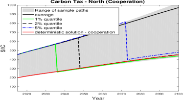
We solve the Bellman equations (16) and (20) with $\psi=1.5$ and $\gamma=3.066$ as our default utility preference values. After we solve the Bellman equations, we use the optimal policy functions to generate 10,000 simulation paths forward. That is, each simulation path starts at the observed initial states, we simulate one sample of the shock for the tipping point at time $t$, and then with the realized sample and the optimal control policy at $t$, we obtain the optimal states at $t+1$.

Figure 2: Regional Carbon Tax

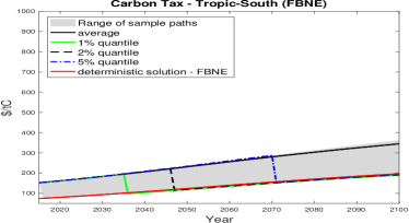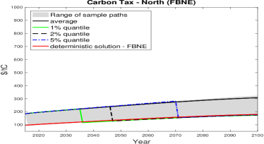
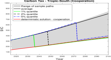
The two left panels of Figure 2 show the distributions of the simulated regional carbon taxes for both regions under the social planner’s model, and the two right panels of Figure 2 are for the feedback Nash equilibrium. All the panels in Figure 2, as well as in the following figures, include a line representing the deterministic case derived with the same IES used in the stochastic model. The shaded area represents the range of the 10,000 sample paths, along with the average, 1%, 2% and 5% quantile paths (that is, at each point in time, we compute the average and these quantiles of 10,000 values). The initial regional carbon tax increases significantly from the deterministic case to the stochastic case under either cooperation or non-cooperation, and the FBNE solution has significantly less regional carbon taxes than the cooperative solution. In the social planner’s problem, the initial regional carbon tax for the stochastic case is $454/tC for the North and $318/tC for the Tropic-South, about 2.3 times that of the corresponding deterministic case (with $\text{$\psi$}=1.5$) with cooperation in each region. In the FBNE, the initial regional carbon tax for the stochastic case is $185/tC for the North and $152/tC for the Tropic-South, more than double of that of the corresponding deterministic case of FBNE in each region, but less than a half of the initial regional carbon tax of the social planner’s stochastic case in each region.

Figure 3: Tipping damage levels and atmospheric carbon concentration

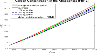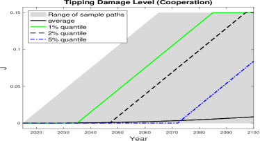
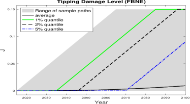
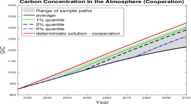
Figure 3 shows the distributions of the optimal simulation paths for tipping damage levels $J_{t}$ and atmospheric carbon concentration under cooperation (the left panels) and non-cooperation (the right panels). For the social planner’s problem, the cumulative probability that the tipping event will occur before 2100 is only 9.6%, while the 1%, 2% and 5% cumulative probability of tipping occurs in years 2035, 2047, and 2072 respectively. For the FBNE, the cumulative probability that the tipping event will occur before 2100 increases to 10.7%, and the 2% or 5% cumulative probability of tipping occurs at an earlier year. Once the tipping event happens, the regional carbon tax immediately falls significantly, but damages unfold over a 50-year period, as shown in the top panels for the tipping damage level $J_{t}$, under both cooperation and non-cooperation. This happens because the high carbon tax before tipping is intended to prevent or delay the tipping point as its occurrence depends on the contemporaneous temperature. However, after the tipping event happens, this incentive disappears as the damage will unfold in a deterministic way. This result is consistent with the finding in DSICE. The bottom panels show that, with the stricter mitigation policy, the stochastic model has smaller carbon concentration in the atmosphere and in 2100 it is on average 200 GtC less than the corresponding deterministic simulation (with $\text{$\psi$}=1.5$) for the cooperative case, and 100 GtC less than the corresponding deterministic FNBE simulation for the noncooperative case. If the tipping event occurs, then the carbon concentration has a higher rate of increase as the corresponding mitigation policy is less strict.

Figure 4: Surface Temperature

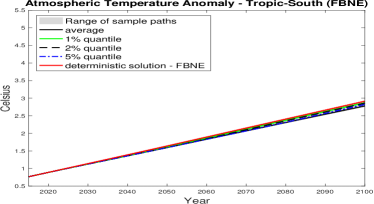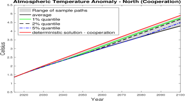
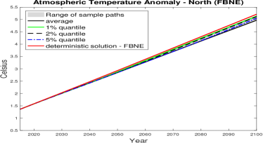
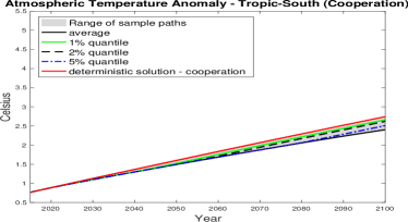
Figure 4 shows the distributions of the optimal simulation paths for atmospheric temperatures in both regions for the cooperative (the left panels) and non-cooperative (the right panels) cases. We see that the North has a much higher temperature anomaly than the Tropic-South. Moreover, the atmospheric temperature anomaly in the North is more than 2℃ higher than in the Tropic-South in 2100. The non-cooperative case has higher temperatures than the cooperative case in both regions, but narrower ranges in 2100.

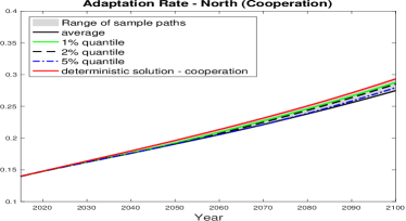
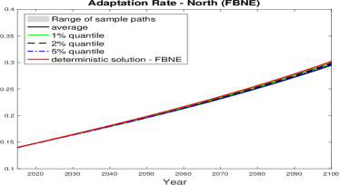
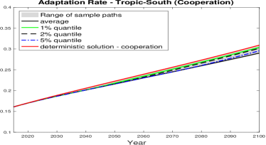
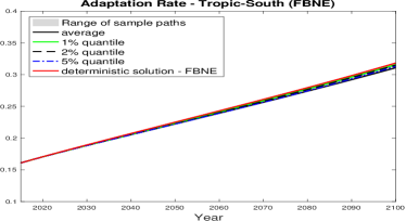
Figure 5 shows the optimal adaptation rates in both regions for the cooperative (the left panels) and non-cooperative (the right panels) cases. We see that the North has lower adaptation rates than the Tropic-South, and that the stochastic results have lower adaptation rates than the corresponding deterministic case, since with the stricter mitigation policy and the resulting lower temperatures in the stochastic case, there is less need to adapt. The non-cooperative case has higher adaptation rates than the cooperative case in both regions, but narrower ranges in 2100. This adaptation policy has a direction between the regions opposite to the carbon tax policy, because the optimal regional adaptation rate is a solution depending only on the regional damage function, the regional mitigation cost function, and the regional adaptation cost function. This can be seen by the FBNE’s first-order condition (A.4) and (A.6), which also hold for the social planner’s problem. That is, adaptation has no direct impact on the common good, carbon concentration. Thus, the cooperation and non-cooperation have no direct impact on adaptation. But since the FBNE has lower carbon tax, which leads to higher temperature and then higher damage, the optimal adaptation is then higher.

Figure 5: Optimal Adaptation

5.1 Bias from Ignoring Heat Transport and PA

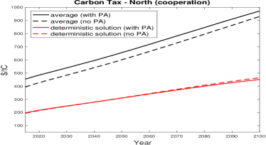
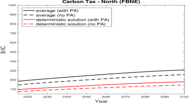
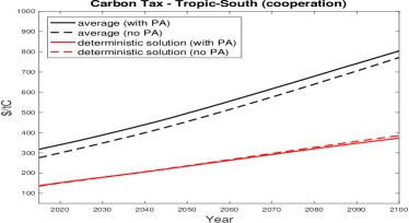
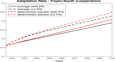
We examine the bias from ignoring heat and moisture transport and PA (i.e., $\xi_{4}=\xi_{5}=0$), shown in Figure 6, for the regional carbon tax under cooperation (the left panels) and non-cooperation (the right panels). In each panel of the figure, the black lines represent the average paths and the red lines represent the solution paths of the deterministic cases. The solid lines show the case with heat and moisture transport and PA, while the dashed lines show the case without it. Figure 6 shows that ignoring heat transport and PA underestimates the average regional carbon taxes for both regions under cooperation and non-cooperation in the initial periods for the stochastic results. For example, the initial regional carbon tax without PA is about 13% less than in the case with PA for both regions in the social planner’s model. This is because ignoring heat transport leads to a lower temperature in the North and then underestimates the tipping probability which depends on the atmospheric temperature in the North. This lower tipping probability means a less risky tipping element which leads to smaller regional carbon taxes. Note that in the deterministic cases, ignoring heat transport has little impact on the regional carbon tax for the social planner’s problem, but in the FBNE, the impact of ignoring heat and moisture transport and PA is in the opposite direction for the regions: it underestimates the regional carbon tax in the North, but a bit overestimates in the Tropic-South.

Figure 6: Bias of Regional Carbon Taxes from Ignoring Heat Transport and PA

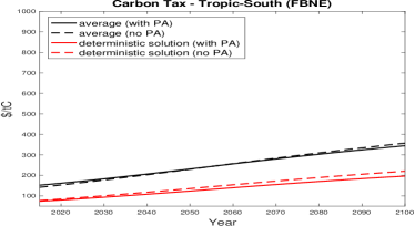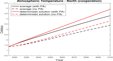
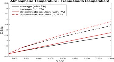
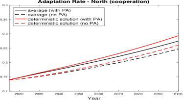
Figure 7 shows that in the social planner’s model ignoring heat transport and PA significantly underestimates the atmospheric temperature anomaly and adaptation rates in the North, and significantly overestimates them in the Tropic-South. The FBNE model has similar pattern so here we omit its figure.

Figure 7: Bias of Temperature and Adaptation from Ignoring Heat Transport and PA

5.2 Bias from Ignoring SLR, Adaptation, and Capital Transfer

Table 1 lists the initial regional carbon tax if we ignore SLR, adaptation, or transfer of capital between regions. Since the FBNE has no capital transfer between regions, Table 1 lists only the cooperative solution. We see that ignoring SLR significantly underestimate the regional carbon taxes. For example, for the social planner’s stochastic model without SLR, the initial regional carbon tax is $294/tC and $207/tC for the North and the Tropic-South respectively, only about 65% of the corresponding ones with SLR. This is because SLR imposes more damage, so it implies higher regional carbon tax. Ignoring adaptation significantly overestimate the regional carbon taxes. For example, for the social planner’s stochastic model without adaptation, the initial regional carbon tax is $855/tC and $601/tC for the North and the Tropic-South respectively, about 88% higher than the corresponding ones with adaptation. This is because adaptation can reduce damages, so it can reduce regional carbon taxes. Ignoring capital transfer (i.e., the closed economy) overestimates the regional carbon taxes for the North and underestimates the regional carbon taxes for the Tropic-South. For example, for the social planner’s stochastic model without capital transfer between regions, the initial regional carbon tax is $540/tC for the North, about 19% higher than the corresponding ones with capital transfer; and in the Tropic-South, the initial regional carbon tax is $275/tC without the capital transfer, about 14% less than the one with the capital transfer. This happens because the capital transfer makes the North to have less capital, then less output and less damages, so the North has less regional carbon taxes; oppositely, the capital transfer makes the Tropic-South to have more capital and then more output and more damages, so the Tropic-South has higher regional carbon taxes. In addition, we also examine the impact of ignoring permafrost thaw and find that it has little impact. The FBNE has the same pattern with the social planner’s solutions for ignoring the elements. Table 1 also shows that the initial regional carbon taxes in the FBNE are always significantly lower than the ones in the cooperative world; the North always has higher regional carbon taxes than the Tropic-South except the deterministic FBNE case without SLR; and the stochastic cases always have higher regional carbon taxes than the deterministic cases, if we ignore SLR, adaptation, or transfer of capital between regions.

Table 1: Initial regional carbon tax from Ignoring Model Elements

Ignored Element	Model	Deterministic		Stochastic
		North	Tropic-South	North	Tropic-South
SLR	Coop.	84	58	294	207
	FBNE	32	33	116	109
Adaptation	Coop.	553	384	855	601
	FBNE	355	214	400	299
Capital Transfer	Coop.	236	118	540	275

5.3 Sensitivity on IES and Risk Aversion

Different values of IES and risk aversion are used in the literature. Table 2 lists the initial regional carbon tax for various IESs $(\psi\in\{0.69,1.5\})$ and risk aversion $(\gamma\in\{3.066,10\})$. Table 2 shows that a higher IES leads to a higher regional carbon tax in both regions; that a higher risk aversion leads to a higher regional carbon tax in both regions; and that stochastic cases have a higher regional carbon tax than deterministic cases for the same IES. This finding is consistent with Cai et al. (forthcoming). Table 2 also shows that for all cases the North has a higher regional carbon tax than the Tropic-South, and the regional carbon taxes in the FBNE are always significantly smaller than the ones in the social planner’s solution.

Table 2: Initial regional carbon tax under various IESs ($\psi$) and risk aversion ($\gamma$)

IES	Model	Deterministic		Stochastic
($\psi$)		North	Tropic	North		Tropic-South
			-South	$\gamma=3.066$	$\gamma=10$	$\gamma=3.066$	$\gamma=10$
0.69	Coop.	58	35	114	132	69	80
	FBNE	29	17	55	63	32	38
1.5	Coop.	198	137	454	519	318	363
	FBNE	90	67	185	208	152	174

6 Conclusion

This paper has taken a first step toward adding heretofore neglected elements – heat and moisture transport from the lower latitudes toward the Poles, sea level rise, adaptation – into computational IAMs used in policy-relevant climate economics. When our model is calibrated to data, we find substantial biases in key quantities such as temperature anomalies, the regional carbon tax and damages, relative to the case where a social planner neglects poleward heat and moisture transport, sea level rise, and adaptation. We also show how potential arrival times of tipping elements in the high latitudes are affected by the transport phenomena and, most importantly, how these tipping elements can affect the regional carbon tax between the two regions.

In our DIRESCU model we have combined the neglected elements with stochastic arrival of tipping points, cooperation and noncooperation between the North and Tropic-South, and recursive preferences which distinguish between risk aversion and the IES. We have shown that these aspects of our model have significant impact on optimal climate policies, so they constitute an important step forward in calibrated IAMs at the “coarse grained” level of aggregation. We have also shown that feedback Nash equilibrium with recursive preferences can be computed in the complex high-dimensional dynamic stochastic model with the advances of computational algorithms and hardware resource.

We expect that future research and extensions in the context of our model – which would involve a finer regional disaggregation, nonlinear surface albedo feedbacks, and better approximations of damages from sources such as SLR or tipping points – could provide additional and improved insights.

Online Appendix for “Climate Policy under Spatial Heat Transport: Cooperative and Noncooperative Regional Outcomes”

Yongyang Cai  William Brock  Anastasios Xepapadeas Kenneth Judd

A.1 Definition of Parameters and Exogenous Paths

In DIRESCU, we approximate the exogenous paths of DICE-2016 in five-year time steps by their annual analogs. The land carbon emissions $E_{t}^{\mathrm{Land}}$ and exogenous radiative forcing $F_{t}^{\mathrm{EX}}$ are defined below:

$$E_{t}^{\mathrm{Land}}=0.95e^{-0.115t}$$ (A.1)

$$F_{t}^{\mathrm{EX}}=\begin{cases}0.5+0.00588t,&\mathrm{if}\;t\leq 85\\ 1,&\mathrm{otherwise}.\end{cases}$$ (A.2)

Tables A.1-A.3 list the values and/or definition of all parameters, variables and symbols.

Table A.1: Parameters, Variables and Symbols in the Deterministic Climate System

$t$	time in years ($t=0$ represents year $2015$)
$i$$\in\{1,2\}$	region $i$ (North or Tropic-South)
$M_{t}^{\mathrm{AT}}$	carbon concentration in the atmosphere (billion tons); $M_{0}^{\mathrm{AT}}=851$
$M_{t}^{\mathrm{UO}}$	carbon concentration in upper ocean (billion tons); $M_{0}^{\mathrm{UO}}=460$
$M_{t}^{\mathrm{DO}}$	carbon concentration in deep ocean (billion tons); $M_{0}^{\mathrm{DO}}=1740$
$\mathbf{M}_{t}=\left(M_{t}^{\mathrm{AT}},M_{t}^{\mathrm{UO}},M_{t}^{\mathrm{DO}}\right)^{\top}$	carbon concentration vector
$T_{t,i}^{\mathrm{AT}}$	average surface temperature (Celsius); $T_{0,1}^{\mathrm{AT}}=1.36$, $T_{0,2}^{\mathrm{AT}}=0.765$
$T_{t}^{\mathrm{OC}}$	average ocean temperature (Celsius); $T_{0}^{\mathrm{OC}}=0.0068$
$\mathbf{T}_{t}=\left(T_{t,1}^{\mathrm{AT}},T_{t,2}^{\mathrm{AT}},T_{t}^{\mathrm{OC}}\right)^{\top}$	temperature vector
$S_{t}$	sea level rise (SLR); $S_{0}=0.14$
$F_{t}$	global radiative forcing
$F_{t}^{\mathrm{EX}}$	exogenous radiative forcing
$\eta=3.68$	radiative forcing parameter
$\mathbf{\Phi}_{\mathrm{M}}$	transition matrix of carbon cycle
$\mathbf{\Phi}_{\mathrm{T}}$	transition matrix of temperature system
$\phi_{1,2}=0.0237$, $\phi_{2,1}=0.0388$	parameters in transition matrix of carbon cycle
$\phi_{2,3}=0.00136$, $\phi_{3,2}=0.00284$	parameters in transition matrix of carbon cycle
$\xi_{1}=0.0526$, $\xi_{2}=0.08987$	parameters in transition matrix of temperature system
$\xi_{3}=0.0022$, $\xi_{4}=0.6557$	parameters in transition matrix of temperature system
$\xi_{5}=0.5565$, $\xi_{6}=0.0$	parameters in transition matrix of temperature system
$\zeta_{1}^{\mathrm{SLR}}=0.00073$, $\zeta_{2}^{\mathrm{SLR}}=1.4$	parameters in SLR by warming
$\zeta_{3}^{\mathrm{SLR}}=0.007$	parameters in SLR by warming
$\zeta_{1}^{\mathrm{Perm}}=1.951$, $\zeta_{2}^{\mathrm{Perm}}=-0.0858$	parameters in emission from permafrost thawing by warming
$\zeta_{3}^{\mathrm{Perm}}=0.2257$	parameters in emission from permafrost thawing by warming
$M_{*}^{\mathrm{AT}}=588$	equilibrium atmospheric carbon concentration

Table A.2: Parameters, Variables and Symbols in the Economic System

$\mathcal{Y}_{t,i}$	gross output
$Y_{t,i}$	output net of damage
$\widehat{Y}_{t,i}$	output net of damage, abatement and adaptation cost
$A_{t,i}$	total productivity factor (TFP); $A_{0,1}=7.331$, $A_{0,2}=3.582$
$\alpha_{1}^{\mathrm{TFP}}=0.013$, $\alpha_{2}^{\mathrm{TFP}}=0.0184$	initial growth of TFP
$d_{1}^{\mathrm{TFP}}=0.0053$, $d_{2}^{\mathrm{TFP}}=0.0061$	change rate of growth of TFP
$L_{t,i}$	population (in billions)
$K_{t,i}$	capital (in $ trillions); $K_{0,1}=146$, $K_{0,2}=77$
$\alpha=0.3$	output elasticity of capital
$D_{t,i}^{\mathrm{S}}$	damage (in fraction of output) from sea level rise
$\pi_{1,1}=0.00447$, $\pi_{1,2}=0.00408$	SLR damage parameter
$\pi_{2,1}=0.01146$, $\pi_{2,2}=0.00646$	SLR damage parameter
$D_{t,i}^{\mathrm{T}}$	damage (in fraction of output) from surface temperature anomaly
$\pi_{3,1}=0.00094$, $\pi_{3,2}=0.00322$	non-SLR damage parameter
$\pi_{4,1}=0.0002$, $\pi_{2,2}=0.00074$	non-SLR damage parameter
$\Psi_{t,i}$	mitigation expenditure
$\Upsilon_{t,i}$	adaptation expenditure
$\mu_{t,i}$	emission control rate
$E_{t}$, $E_{t,i}^{\mathrm{Ind}}$, $E_{t}^{\mathrm{Land}}$	global emission; regional industrial emission; land emission
$P_{t,i}$	adaptation rate
$\sigma_{t,i}$	carbon intensity; $\sigma_{0,1}=0.094$, $\sigma_{0,2}=0.104$
$\alpha_{1}^{\sigma}=0.0156$, $\alpha_{2}^{\sigma}=0.0181$	initial declining rate of carbon intensity
$d_{1}^{\sigma}=0.0063$, $d_{2}^{\sigma}=0.007$	change rate of growth of carbon intensity
$\theta_{2}=2.6$	mitigation cost parameter
$\theta_{1,t,i}$	adjusted cost for backstop
$b_{0,1}=1.71$, $b_{0,2}=2.19$	initial backstop price
$\alpha_{1}^{b}=\alpha_{2}^{b}=0.005$	declining rate of backstop price
$\eta_{1}=0.115$, $\eta_{2}=3.6$	parameters for adaptation cost
$\delta=0.1$	annual depreciation rate
$c_{t,i}$	per capita consumption
$I_{t,i}$	investment
$\Gamma_{t,i}$	adjustment cost for economic interaction between regions
$B=1$	parameter for economic interaction cost
$\psi\in\{0.69,1.5\}$	IES
$u$	per capita utility function
$\beta=0.985$	discount factor

Table A.3: Additional Parameters, Variables and Symbols in the Stochastic Model

$D=50$	duration of tipping process
$J_{t}$	damage level; $J_{0}=0$
$\overline{J}=0.15$	final damage level
$\Delta$	annual increment of damage level
$\chi_{t}\in\{0,1\}$	indicator for whether tipping has happened; $\chi_{0}=0$
$p_{t}$	tipping probability
$\varrho=0.00063$	hazard rate for tipping
$\gamma\in\{3.066,10\}$	risk aversion parameter
$\mathbf{x}_{t}$	vector of state variables
$V_{t}$	value function at time $t$
$V_{t}^{\mathrm{SP}}$	value function for the social planner’s problem
$V_{t}^{\mathrm{FBNE}}$	value function for the feedback Nash equilibrium problem

A.2 Calibration of the Climate System

Figure A.1 shows that our calibrated carbon cycle can approximate well for all scenarios except RCP8.5. Since RCP8.5 is the business-as-usual scenario, and our model is solving problems with optimal mitigation policy, the deviation of approximation for RCP8.5 has little impact on our solutions.

Figure A.1: Fitting Atmospheric Carbon Concentration

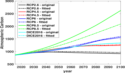
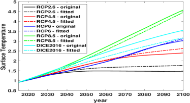
Figure A.2 shows that our calibrated temperature system can approximate well for all these scenarios. Figure A.3 displays the corresponding spatial surface temperature and ocean temperature pathways from the calibrated temperature system, for the RCP scenarios and the DICE-2016 optimal scenario. It also shows that the spatial surface temperatures in 2081-2100 are close to the ones given in IPCC (2013).

Figure A.2: Fitting Surface Temperature

Figure A.3: Spatial Temperature Using RCP or DICE Radiative Forcing Scenarios

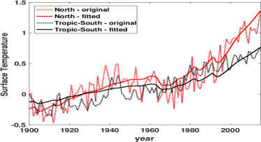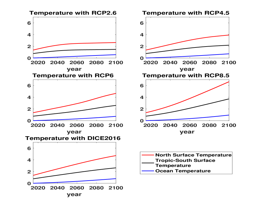
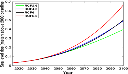
Figure A.4 shows that our fitted paths of SLR (above the level in 2000) for RCP2.6, RCP4.5 and RCP6 are quite close to the mean projections in IPCC (2013) and Kopp et al. (2014).

Figure A.4: Fitting SLR

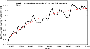
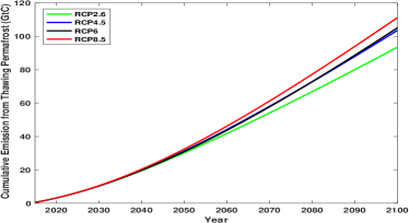
The left panel of Figure A.5 shows that our function (5) for estimating emissions from thawing permafrost fits data well, and the right panel of Figure A.5 shows projected future cumulative emission paths from thawing permafrost since 2010 for four RCP scenarios. We see that the cumulative carbon emission under RCP8.5 is also inside the likely range given in Schuur et al. (2015).

Figure A.5: Fitting the Carbon Emission Data from Thawing Permafrost and Projecting Future Cumulative Emission Paths from Thawing Permafrost since 2010

A.3 Calibration of the Economic System

The left panel of Figure A.6 shows that our calibrated TFP paths match RICE projections over both the North and the Tropic-South. The right panel of Figure A.6 shows that our carbon intensity estimate (11) closely approximates the corresponding RICE projections.

Figure A.6: Fitting Total Factor Productivity (the left panel) and Carbon Intensity (the right panel)

The left panel of Figure A.7 shows that our estimate of SLR damage function (9) is close to the RICE projection of SLR damage for both the North and the Tropic-South. The right panel of Figure A.7 shows that our non-SLR damage functions (10) fit the RICE projection of non-SLR damage in fraction of output.

Figure A.7: Fitting SLR Damage (the left panel) and non-SLR Damage (the right panel) to Output

A.4 First Order Conditions for FBNE

The system of first-order conditions (23) represents the following equations:

$$0 = u^{\prime}(c_{t,i})-\beta\frac{\partial\mathcal{G}_{t,i}(\mathbf{x}_{t+1})}{\partial K_{t+1,i}},\ i=1,2,$$ (A.3)

$$0 = \frac{\partial\widehat{Y}_{t,i}}{\partial P_{t,i}},\ i=1,2,$$ (A.4)

$$0 = \frac{\partial\mathcal{G}_{t,i}(\mathbf{x}_{t+1})}{\partial K_{t+1,i}}\frac{\partial\widehat{Y}_{t,i}}{\partial\mu_{t,i}}+\frac{\partial\mathcal{G}_{t,i}(\mathbf{x}_{t+1})}{\partial M_{t+1}^{\mathrm{AT}}}\frac{\partial E_{t,i}^{\mathrm{Ind}}}{\partial\mu_{t,i}},\ i=1,2,$$ (A.5)

where we use $\frac{\partial K_{t+1,i}}{\partial c_{t,i}}=-L_{t,i}$ in deriving (A.3), and $\frac{\partial K_{t+1,i}}{\partial\widehat{Y}_{t,i}}=1$ and $\frac{\partial M_{t+1}^{\mathrm{AT}}}{\partial E_{t,i}^{\mathrm{Ind}}}=1$ in deriving (A.5).

Here,

$$\frac{\partial\mathcal{G}_{t,i}(\mathbf{x}_{t+1})}{\partial K_{t+1,i}} = \left[\mathbb{E}_{t}\left(\left(V_{t+1,i}^{\mathrm{FBNE}}(\mathbf{x}_{t+1})\right)^{\varTheta}\right)\right]^{1/\varTheta-1}\mathbb{E}_{t}\left(\left(V_{t+1,i}^{\mathrm{FBNE}}(\mathbf{x}_{t+1})\right)^{\varTheta-1}\frac{\partial V_{t+1,i}^{\mathrm{FBNE}}(\mathbf{x}_{t+1})}{\partial K_{t+1,i}}\right)$$

$$\frac{\partial\mathcal{G}_{t,i}(\mathbf{x}_{t+1})}{\partial M_{t+1}^{\mathrm{AT}}} = \left[\mathbb{E}_{t}\left(\left(V_{t+1,i}^{\mathrm{FBNE}}(\mathbf{x}_{t+1})\right)^{\varTheta}\right)\right]^{1/\varTheta-1}\mathbb{E}_{t}\left(\left(V_{t+1,i}^{\mathrm{FBNE}}(\mathbf{x}_{t+1})\right)^{\varTheta-1}\frac{\partial V_{t+1,i}^{\mathrm{FBNE}}(\mathbf{x}_{t+1})}{\partial M_{t+1}^{\mathrm{AT}}}\right)$$

$$\frac{\partial\widehat{Y}_{t,i}}{\partial P_{t,i}} = Y_{t,i}\left[\left(1-\theta_{1,t,i}\mu_{t,i}^{\theta_{2}}-\eta_{1}P_{t,i}^{\eta_{2}}\right)\Omega_{t,i}(D_{t,i}^{\mathrm{SLR}}+D_{t,i}^{\mathrm{T}})-\eta_{1}\eta_{2}P_{t,i}^{\eta_{2}-1}\right]$$ (A.6)

$$\frac{\partial\widehat{Y}_{t,i}}{\partial\mu_{t,i}} = -\theta_{1,t,i}\theta_{2}\mu_{t,i}^{\theta_{2}-1}Y_{t,i}$$

$$\frac{\partial E_{t,i}^{\mathrm{Ind}}}{\partial\mu_{t,i}} = -\sigma_{t,i}\mathcal{Y}_{t,i}$$

by assuming $\psi>1$ for convenience. When $\psi<1$, we just need to replace $\beta$ by $-\beta$, and $V_{t+1,i}^{\mathrm{FBNE}}$ by $-V_{t+1,i}^{\mathrm{FBNE}}$ in the equations.

A.5 No Transfer of Capital in the FBNE

In the FBNE, region $i$ chooses $I_{t,i},c_{t,i},\mu_{t,i},P_{t,i}$, and migrated capital from the region $i$ to the other. Let $\Delta_{t,1}\geq 0$ be migrated capital from region 1 o 2, and $\Delta_{t,2}\geq 0$ from region 2 o 1. Assume the IES $\psi<1$ for convenience. The FBNE solves

$$V_{t,i}(\mathbf{x}_{t})=\max_{I_{t,i},c_{t,i},\mu_{t,i},P_{t,i},\Delta_{t,i}\geq 0}\left\{u(c_{t,i})L_{t,i}+\beta\mathcal{G}_{t,i}(\mathbf{x}_{t+1})\right\},$$ (A.7)

for $i=1,2$, subject to the transition laws (1), (3), (4), (13), (6), (7), and the following region-specific market clearing constraint

$$I_{t,1}+c_{t,1}L_{t,1}+\Gamma_{t,1}-\Delta_{t,1}+\Delta_{t,2} = \widehat{Y}_{t,1}$$ (A.8)

$$I_{t,2}+c_{t,2}L_{t,2}+\Gamma_{t,2}+\Delta_{t,1}-\Delta_{t,2} = \widehat{Y}_{t,2}$$ (A.9)

respectively, where

$$\Gamma_{t,i}=\frac{B}{2}\widehat{Y}_{t,i}\left(\frac{\Delta_{t,1}+\Delta_{t,2}}{\widehat{Y}_{t,i}}\right)^{2}$$

Let $\lambda_{t,i}\geq 0$ be shadow prices for (A.8) and (A.9), and $\tau_{t,i}\geq 0$ for $\Delta_{t,i}\geq 0$, for $i=1,2$. Then from the KKT conditions of (A.7) for region $i$, we have

$$u^{\prime}(c_{t,i}) = \lambda_{t,i}$$

$$\lambda_{t,i}\left(1-\frac{\partial\Gamma_{t,i}}{\partial\Delta_{t,i}}\right) = \tau_{t,i}$$

$$\tau_{t,i}\Delta_{t,i} = 0$$

Thus, since $\lambda_{t,i}=u^{\prime}(c_{t,i})>0$ and $\frac{\partial\Gamma_{t,i}}{\partial\Delta_{t,i}}=B\frac{\Delta_{t,1}+\Delta_{t,2}}{\widehat{Y}_{t,i}}<1$ (as $B=1$ and it is impossible to have $\Delta_{t,1}+\Delta_{t,2}\geq Y_{t,i}$ due to our regional specification), we have $\tau_{t,i}>0$ and then $\Delta_{t,i}=0$. That is, in the FBNE, there is no transfer of capital between the regions.

A.6 $L^{1}$ fitting

It is typical to choose the $\mathcal{L}^{1}$ norm in the minimization step of Algorithm 1. In this case, we can avoid the kinks by transforming the minimization model (26) to

$$\min \sum_{i,k}(\epsilon^{\prime}_{i,1,k}+\epsilon^{\prime}_{i,2,k}),$$ (A.10)

$$\mathrm{s.t.} \nabla_{\mathbf{a}}\left(u_{t,i}(\mathbf{x},\mathbf{a})+\beta\mathcal{G}_{t,i}\left(\mathbf{H}_{t}(\mathbf{x},\mathbf{a},\omega)\right)\right)=\mathbf{\epsilon^{\prime}}_{i,1}-\mathbf{\epsilon}^{\prime}_{i,2},\ i\in\mathbb{I},$$

$$\mathbf{a}\in\mathcal{D}(\mathbf{x},t),$$

$$0\leq\epsilon^{\prime}_{i,j,k}\leq\bar{\epsilon}^{\prime},\ i\in\mathbb{I};j=1,2;k=1,...,n,$$

where $\epsilon^{\prime}_{i,1},\epsilon^{\prime}_{i,2}$ are length-$n$ nonnegative vectors, $\epsilon^{\prime}_{i,1,k},\epsilon^{\prime}_{i,2,k}$ are their elements, and $\bar{\epsilon}^{\prime}$ is a small positive number. To reduce computational time, we may instead solve the following problem

$$\min \sum_{i,k}\epsilon^{\prime\prime}_{i,k},$$ (A.11)

$$\mathrm{s.t.} \nabla_{\mathbf{a}}\left(u_{t,i}(\mathbf{x},\mathbf{a})+\beta\mathcal{G}_{t,i}\left(\mathbf{H}_{t}(\mathbf{x},\mathbf{a},\omega)\right)\right)=\mathbf{\epsilon}^{\prime\prime}_{i},\ i\in\mathbb{I},$$

$$\mathbf{a}\in\mathcal{D}(\mathbf{x},t),$$

$$0\leq\epsilon^{\prime\prime}_{i,k}\leq\bar{\epsilon}^{\prime\prime},\ i\in\mathbb{I};k=1,...,n$$

where $\epsilon^{\prime\prime}_{i}$ is a length-$n$ nonnegative vector, $\epsilon^{\prime\prime}_{i,k}$ are its elements, and $\bar{\epsilon}^{\prime\prime}$ is a small positive number.

A.7 Terminal Value Function

For the social planner’s problem, the terminal value function at the terminal time $T=300$ (i.e., year 2315) is computed as

$$V_{T}^{\mathrm{SP}}(\mathbf{x}_{T})=\sum_{i=1}^{2}\sum_{t=300}^{600}\beta^{t-300}u(c_{t,i})L_{T,i},$$

where we assume that for all $t>T$, all exogenous paths stop changing and fix their values at terminal time $T$. Emission control rates are always 1 (i.e., $\mu_{t,i}=1$), adaptation rates are fixed at a constant level, there are no economic interaction costs (i.e., $\Gamma_{t,i}=0$), and both $c_{t,i}L_{t,i}/Y_{t,i}$ and $I_{t,i}/Y_{t,i}$ are given constant values. Moreover, we assume that if the tipping event has not happened before $T$, then it never happens; or if the tipping event has happened, then its damage will unfold until its maximum level.

For the FBNE, the terminal value functions at $T=300$ are computed as

$$V_{T,i}^{\mathrm{FBNE}}(\mathbf{x}_{T})=\sum_{t=300}^{600}\beta^{t-300}u(c_{t,i})L_{T,i}$$

for $i=1,2$, under the same assumptions of the social planner’s problem for periods after $T=300$. In both cooperative and noncooperative cases, consideration of alternatives showed that changes in the terminal value functions at year 2315 had no significant impact on any results for the twenty-first century.

References

- Anderson and van Wincoop (2003) Anderson, J. E. and E. van Wincoop (2003): “Gravity with Gravitas: A Solution to the Border Puzzle,” American Economic Review, 93, 170–192.
- Bamber et al. (2009) Bamber, J. L., R. E. M. Riva, B. L. A. Vermeersen, and A. M. LeBrocq (2009): “Reassessment of the Potential Sea-Level Rise from a Collapse of the West Antarctic Ice Sheet,” Science, 324, 901–903.
- Bansal et al. (2016) Bansal, R., D. Kiku, and M. Ochoa (2016): “Price of Long-Run Temperature Shifts in Capital Markets,” Working Paper 22529, National Bureau of Economic Research.
- Bansal and Yaron (2004) Bansal, R. and A. Yaron (2004): “Risks for the Long Run: A Potential Resolution of Asset Pricing Puzzles,” The Journal of Finance, 59, 1481–1509.
- Barreca et al. (2016) Barreca, A., K. Clay, O. Deschenes, M. Greenstone, and J. S. Shapiro (2016): “Adapting to Climate Change: The Remarkable Decline in the US Temperature-Mortality Relationship over the Twentieth Century,” Journal of Political Economy, 124, 105–159.
- Basar and Olsder (1999) Basar, T. and G. J. Olsder (1999): Dynamic Noncooperative Game Theory (2nd Edition), Society for Industrial and Applied Mathematics.
- Bekryaev et al. (2010) Bekryaev, R. V., I. V. Polyakov, and V. A. Alexeev (2010): “Role of polar amplification in long-term surface air temperature variations and modern Arctic warming,” Journal of Climate, 23, 3888–3906.
- Brock and Xepapadeas (2017) Brock, W. and A. Xepapadeas (2017): “Climate change policy under polar amplification,” European Economic Review, 94, 263–282.
- Burgess et al. (2014) Burgess, R., O. Deschenes, D. Donaldson, and M. Greenstone (2014): “The unequal effects of weather and climate change: Evidence from mortality in india,” Working paper.
- Burke et al. (2015) Burke, M., S. M. Hsiang, and E. Miguel (2015): “Global non-linear effect of temperature on economic production,” Nature, 527, 235–239.
- Cai (forthcoming) Cai, Y. (forthcoming): “Computational methods in environmental and resource economics,” Annual Review of Resource Economics.
- Cai et al. (2018a) Cai, Y., K. L. Judd, and T. S. Lontzek (2018a): “Numerical dynamic programming with verification and uncertainty quantification: an application to climate policy,” Working paper.
- Cai et al. (forthcoming) ——— (forthcoming): “The social cost of carbon with economic and climate risks,” Journal of Political Economy.
- Cai et al. (2015) Cai, Y., K. L. Judd, G. Thain, and S. Wright (2015): “Solving dynamic programming problems on computational grid,” Computational Economics, 45, 261–284.
- Cai et al. (2016) Cai, Y., T. M. Lenton, and T. S. Lontzek (2016): “Risk of multiple interacting tipping points should encourage rapid CO2 emission reduction,” Nature Climate Change, 6, 520–525.
- Cai et al. (2018b) Cai, Y., H. Selod, and J. Steinbuks (2018b): “Urbanization and land property rights,” Regional Science and Urban Economics, 70, 246–257.
- Cohen et al. (2018) Cohen, J., K. Pfeiffer, and J. A. Francis (2018): “Warm Arctic episodes linked with increased frequency of extreme winter weather in the United States,” Nature Communications, 9, 869.
- de Bruin et al. (2009) de Bruin, K. C., R. B. Dellink, and R. S. J. Tol (2009): “AD-DICE: an implementation of adaptation in the DICE model,” Climatic Change, 95, 63–81.
- Dell et al. (2012) Dell, M., B. F. Jones, and B. A. Olken (2012): “Temperature Shocks and Economic Growth: Evidence from the Last Half Century,” American Economic Journal: Macroeconomics, 4, 66–95.
- Eaton and Kortum (2002) Eaton, J. and S. Kortum (2002): “Technology, Geography, and Trade,” Econometrica, 70, 1741–1779.
- Engwerda (2009) Engwerda, J. (2009): Linear Quadratic Differential Games: An Overview, Boston: Birkhäuser Boston, 1–34.
- Epstein and Zin (1989) Epstein, L. G. and S. E. Zin (1989): “Substitution, Risk Aversion, and the Temporal Behavior of Consumption and Asset Returns: A Theoretical Framework,” Econometrica, 57, 937–969.
- GISTEMP Team (2018) GISTEMP Team (2018): “GISS Surface Temperature Analysis (GISTEMP). NASA Goddard Institute for Space Studies,” Accessed on March 7, 2018.
- Golosov et al. (2014) Golosov, M., J. Hassler, P. Krusell, and A. Tsyvinski (2014): “Optimal Taxes on Fossil Fuel in General Equilibrium,” Econometrica, 82, 41–88.
- Goulder et al. (2016) Goulder, L. H., M. A. C. Hafstead, and I. Williams, Roberton C. (2016): “General Equilibrium Impacts of a Federal Clean Energy Standard,” American Economic Journal: Economic Policy, 8, 186–218.
- Hassler and Krusell (2012) Hassler, J. and P. Krusell (2012): “Economics and climate change: integrated assessment in a multi-region world,” Journal of the European Economic Association, 10, 974–1000.
- Hope and Schaefer (2016) Hope, C. and K. Schaefer (2016): “Economic impacts of carbon dioxide and methane released from thawing permafrost,” Nature Climate Change, 6, 56–59.
- Hsiang et al. (2017) Hsiang, S., R. Kopp, A. Jina, J. Rising, M. Delgado, S. Mohan, D. J. Rasmussen, R. Muir-Wood, P. Wilson, M. Oppenheimer, K. Larsen, and T. Houser (2017): “Estimating economic damage from climate change in the United States,” Science, 356, 1362–1369.
- IPCC (2007) IPCC (2007): Climate Change 2007, The Physical Science Basis, New York: Cambridge University Press.
- IPCC (2013) ——— (2013): Climate Change 2013, The Physical Science Basis, New York: Cambridge University Press.
- Jaakkola and van der Ploeg (2018) Jaakkola, N. and F. van der Ploeg (2018): “Non-cooperative and cooperative climate policies with anticipated breakthrough technology,” Journal of Environmental Economics and Management.
- Judd (1992) Judd, K. L. (1992): “Projection Methods for Solving Aggregate Growth Models,” Journal of Economic Theory, 58, 410–452.
- Judd (1998) ——— (1998): Numerical Methods in Economics, The MIT Press.
- Kopp et al. (2014) Kopp, R. E., R. M. Horton, C. M. Little, J. X. Mitrovica, M. Oppenheimer, D. J. Rasmussen, B. H. Strauss, and C. Tebaldi (2014): “Probabilistic 21st and 22nd century sea-level projections at a global network of tide-gauge sites,” Earth’s Future, 2, 383–406.
- Krusell and Smith (2017) Krusell, P. and A. Smith (2017): “Climate Change Around the World,” memo.
- Langen and Alexeev (2007) Langen, P. L. and V. A. Alexeev (2007): “Polar amplification as a preferred response in an idealized aquaplanet GCM,” Climate Dynamics, 29, 305–317.
- Lemoine and Traeger (2014) Lemoine, D. and C. Traeger (2014): “Watch Your Step: Optimal Policy in a Tipping Climate,” American Economic Journal: Economic Policy, 6, 137–166.
- Lenton and Schellnhuber (2007) Lenton, T. M. and H. J. Schellnhuber (2007): “Tipping the scales,” Nature Reports Climate Change, 1, 97–98.
- Meinshausen et al. (2011a) Meinshausen, M., S. Raper, and T. Wigley (2011a): “Emulating coupled atmosphere-ocean and carbon cycle models with a simpler model, MAGICC6: Part I - Model Description and Calibration,” Atmospheric Chemistry and Physics, 11, 1417–1452.
- Meinshausen et al. (2011b) Meinshausen, M., S. Smith, K. Calvin, J. Daniel, M. Kainuma, J.-F. Lamarque, K. Matsumoto, S. Montzka, S. Raper, K. Riahi, A. Thomson, G. Velders, and D. van Vuuren (2011b): “The RCP greenhouse gas concentrations and their extensions from 1765 to 2300,” Climatic Change, 109, 213–241.
- Miranda and Fackler (2002) Miranda, M. J. and P. L. Fackler (2002): Applied Computational Economics and Finance, The MIT Press.
- Nerem et al. (2018) Nerem, R. S., B. D. Beckley, J. T. Fasullo, B. D. Hamlington, D. Masters, and G. T. Mitchum (2018): “Climate-change–driven accelerated sea-level rise detected in the altimeter era,” Proceedings of the National Academy of Sciences.
- Nordhaus (2010) Nordhaus, W. D. (2010): “Economic aspects of global warming in a post-Copenhagen environment,” Proceedings of the National Academy of Sciences, 107, 11721–11726.
- Nordhaus (2017) ——— (2017): “Revisiting the social cost of carbon,” Proceedings of the National Academy of Sciences of the United States of America, 114, 1518–1523.
- Overland and Wang (2018) Overland, J. E. and M. Wang (2018): “Arctic-midlatitude weather linkages in North America,” Polar Science.
- Pakes and McGuire (1994) Pakes, A. and P. McGuire (1994): “Computing Markov-Perfect Nash Equilibria: Numerical Implications of a Dynamic Differentiated Product Model,” RAND Journal of Economics, 25, 555–589.
- Pindyck and Wang (2013) Pindyck, R. S. and N. Wang (2013): “The Economic and Policy Consequences of Catastrophes,” American Economic Journal: Economic Policy, 5, 306–339.
- Rui and Miranda (1996) Rui, X. and M. Miranda (1996): “Solving nonlinear dynamic games via orthogonal collocation: An application to international commodity markets,” Annals of Operations Research, 68, 89–108.
- Sachs (2001) Sachs, J. D. (2001): “Tropical Underdevelopment,” Working Paper 8119, National Bureau of Economic Research.
- Sachs and McArthur (2002) Sachs, J. D. and J. W. McArthur (2002): “Technology and the New Economy,” Cambridge, MA, USA: MIT Press, chap. Technological Advancement and Long-term Economic Growth in Asia, 157–185.
- Schuur et al. (2015) Schuur, E. A. G., A. D. McGuire, C. Schadel, G. Grosse, J. W. Harden, D. J. Hayes, G. Hugelius, C. D. Koven, P. Kuhry, D. M. Lawrence, S. M. Natali, D. Olefeldt, V. E. Romanovsky, K. Schaefer, M. R. Turetsky, C. C. Treat, and J. E. Vonk (2015): “Climate change and the permafrost carbon feedback,” Nature, 520, 171–179.
- van der Ploeg and de Zeeuw (2016) van der Ploeg, F. and A. de Zeeuw (2016): “Non-cooperative and Cooperative Responses to Climate Catastrophes in the Global Economy: A North-South Perspective,” Environmental and Resource Economics, 65, 519–540.