Dynamical correlations and pairwise theory for the symbiotic contact process on networks

Abstract

The two-species symbiotic contact process (2SCP) is a stochastic process where each vertex of a graph may be vacant or host at most one individual of each species. Vertices with both species have a reduced death rate, representing a symbiotic interaction, while the dynamics evolves according to the standard (single species) contact process rules otherwise. We investigate the role of dynamical correlations on the 2SCP on homogeneous and heterogeneous networks using pairwise mean-field theory. This approach is compared with the ordinary one-site theory and stochastic simulations. We show that our approach significantly outperforms the one-site theory. In particular, the stationary state of the 2SCP model on random regular networks is very accurately reproduced by the pairwise mean-field, even for relatively small values of vertex degree, where expressive deviations of the standard mean-field are observed. The pairwise approach is also able to capture the transition points accurately for heterogeneous networks and provides rich phase diagrams with transitions not predicted by the one-site method. Our theoretical results are corroborated by extensive numerical simulations.

I Introduction

Discontinuous transitions D’Souza et al. (2019), observed in distinct classes of cooperative systems, have lifted a renewed burst of interest within different contexts such as social interactions Perc et al. (2017); Gómez-Gardeñes et al. (2016), coinfections Wang et al. (2019); Cai et al. (2015); Grassberger et al. (2016), synchronization Boccaletti et al. (2016); D’Souza et al. (2019), and percolation Boccaletti et al. (2016); D’Souza et al. (2019), to cite only a few fundamental processes. A leading part of these investigations is addressed to phenomena occurring on the top of complex networks Albert and Barabási (2002), that constitute basic substrates for describing interacting patterns of complex systems Pastor-Satorras et al. (2015); Castellano et al. (2009); Ohtsuki et al. (2006). While in a continuous transition the order parameter varies continuously from zero, in the discontinuous case it suddenly jumps to a finite value at the transition point, involving a macroscopic portion of the system and this transition is commonly refereed as catastrophic or abrupt Strogatz (2018).

Coinfection epidemics Wang et al. (2019), when a host can be infected simultaneously by two distinct diseases, can result in coexisting thresholds when competitive interactions are considered Newman (2005); Newman and Ferrario (2013). Nevertheless, cooperative or synergistic interactions result in richer phase diagrams, which may include discontinuous phase transitions, and have been a topic of intense research Newman and Ferrario (2013); Chen et al. (2013, 2013); Cai et al. (2015); Grassberger et al. (2016); Janssen and Stenull (2016); Cui et al. (2017); Liu et al. (2017). Cooperation and competition have been investigated on multi-species interacting models in distinct ecological contexts Tubay et al. (2013); Dobramysl and Täuber (2013); Court et al. (2013); Markham et al. (2013); Iwata et al. (2011); De Oliveira et al. (2012). Particularly, symbiotic interactions were recently investigated in a two-species contact process (2SCP) De Oliveira et al. (2012). In the standard, single-species contact process (CP) Harris (1974), individuals lay on the vertices of a graph, which was originally a lattice, but it was later extended to networks Castellano and Pastor-Satorras (2006); Ferreira et al. (2011). In the standard CP model, each individual can reproduce asexually with rate $\lambda$, with its offspring occupying one empty nearest-neighbor randomly chosen, or die with rate $\mu$ (which can be taken as $\mu=1$ without loss of generality). In the 2SCP De Oliveira et al. (2012), two species, A and B, inhabit the same graph. The symbiotic interaction is modeled via a reduced death rate, $\mu<1$, at sites doubly occupied (by one individual of each species). With the exception of this interaction, the two populations evolve independently according to the standard CP.

Apart from its interest as an elementary model of symbiosis, the 2SCP is fundamentally interesting for the study of nonequilibrium phase transitions. Extinction represents an absorbing state, i.e., a frozen state without fluctuations of populations Marro and Dickman (2005). On regular lattices, it was found that the 2SCP exhibits a continuous phase transition in one and two dimensions De Oliveira et al. (2012). However, the transition becomes discontinuous in the regime of strong symbiosis if diffusion is introduced de Oliveira and Dickman (2014). The 2SCP was recently investigated in complete graphs and random regular networks Sampaio Filho et al. (2018) and it was conjectured that the nature of its transition changes at the upper critical dimension, from continuous to discontinuous. The phase diagram determining the regions of the 2SCP’ space parameter $\mu$ versus $\lambda$ was determined in the ordinary, one-site mean-field level De Oliveira et al. (2012); de Oliveira and Dickman (2014); Sampaio Filho et al. (2018), which neglects all dynamical correlations with the assumption of statistical independence among the states of individuals even if they are nearest-neighbors. This assumption is a strong approximation that can make the theory inaccurate even for high dimensional systems such as the complex networks Gleeson (2011), where the small-world property Albert and Barabási (2002) resembles a mean-field (fully connected) regime. Dynamical correlations can be introduced using pairwise approximations Marro and Dickman (2005); Ben-Avraham and Köhler (1992) where the mean-field equations for pairs of connected vertices are considered. Even still being inaccurate in low dimensions Marro and Dickman (2005), pairwise correlations highly improve the theoretical results in the case of dynamical processes on complex networks Keeling (1999); Eames and Keeling (2002); Gleeson (2011, 2013); Mata et al. (2014).

In the present work, we investigate the role of dynamical correlations in the 2SCP using a homogeneous pairwise mean-field (PMF) theory. The theoretical predictions are compared with stochastic simulations on different random networks, including homogeneous, Poissonian, and scale-free degree distributions Barabási and Albert (1999). We observe that the PMF theory substantially improves the ordinary mean-field in all investigated cases, being very accurate for determining the transition points and phase diagrams. Moreover, the PMF phase diagrams are more complex, showing discontinuous transitions with either symbiosis parameter $\mu$ or rate infection $\lambda$ fixed in contrast with the ordinary mean-field where only the former one can happen.

The remainder of this paper is organized as follows. In Sec. II we present the definitions of the model and networks used as substrates for simulations. The mean-field theories are developed in Sec. III and Appendix A while the simulation methods used in the present work are described in Sec IV. Section V is devoted to the comparison between mean-field theories and simulation outcomes. Finally, our conclusions and prospects are drawn in Sec. VI.

II Model and networks

We investigate the symmetric 2SCP De Oliveira et al. (2012), in which the involved rates are the same for both species. The model is defined for a networked substrate as follows. Each vertex of the network can hold at most one individual of each species A and B. So, the state $S$ of a vertex $i$ can be empty, represented by $S_{i}=\times$, occupied by only one individual of type A ($S_{i}=\circ$) or B ($S_{i}=\bullet$), or occupied by one individual of each species, represented by $S_{i}={\circ\bullet}$. The reproduction of new individuals of a given species happens independently of each other according to the standard CP rules Marro and Dickman (2005); Harris (1974). A vertex $i$ with one individual of type A, $S_{i}=\circ$ or $S_{i}={\circ\bullet}$, creates an offspring of type A at a randomly selected nearest-neighbor $j$ with rate $\lambda$ if $j$ does not have an individual of type A (i.e., if $S_{j}=\times$ or $S_{j}=\bullet$). Same rules and rates are used for the replication of a type B. Any individual in a vertex $i$ spontaneously dies with rate 1 if they are alone ($S_{i}=\circ$ or $\bullet$) or with rate $\mu$, otherwise ($S_{i}={\circ\bullet}$). If $\mu=1$ the two processes evolve independently, but for $\mu<1$ they interact symbiotically since the annihilation rates are reduced at vertices where both species are present. The stationary 2SCP can evolve asymptotically to a fully active state, where there is coexistence of both species or to an inactive (absorbing) phase in which both species are extinct. There are also two partly active states, where only one of A or B species are extinct that can be reached for specific initial conditions (the dynamics in these partly active states is out of our interest since it is that of a standard single-species CP).

In this work, we use random graph models as substrates on which the 2SCP takes place. The number of neighbors of a vertex $i$, the vertex degree, is denoted by $k_{i}$. We consider both homogeneous and heterogeneous networks. In random regular (RR) networks Ferreira and Ferreira (2013) all vertices have the same degree $k_{i}=k$ and connections are performed at random following the configuration model Catanzaro et al. (2005) avoiding both multiple and self connections. In the Erdös-Renyi (ER) model Albert and Barabási (2002), each pair of vertices is connected with probability $p$. When the size of the graph $N\to\infty$, its degree distribution is a Poissonian with a finite mean $\langle{k}\rangle=pN$. Both RR and ER models belong to the class of homogeneous degree networks, where large deviations from the average value do not occur Barabási and Pósfai (2016), whereas only RR has a strictly homogeneous degree distribution. The third substrate is the Barabási-Albert (BA) model Barabási and Albert (1999), in which the networks are generated through a preferential attachment mechanism Barabási and Albert (1999) starting from a fully connected set with $m_{0}+1$ vertices and vertices with $m$ edges being added one at a time. We used $m=m_{0}$ such that the average degree $\langle{k}\rangle=m$ can be fixed accordingly for comparison with the homogeneous case. The BA degree distribution follows asymptotically a power law (PL), $p_{k}\sim k^{-\gamma}$, with $\gamma=3$ and is representative of a highly heterogeneous network possessing a heavy-tailed degree distribution.

III Mean-field theory

We consider a homogeneous mean-field approximation where all vertices are assumed to have the same degree $k_{i}=k$. In order to apply this theory to heterogeneous cases of ER and BA we use the same equations of the homogeneous theory replacing $k$ by $\langle{k}\rangle$. This strategy has been used to compare the transition points of CP obtained in a homogeneous PMF theory, given by $\lambda_{\text{c}}=k/(k-1)$ Marro and Dickman (2005), with the simulations on heterogeneous networks using $\lambda_{\text{c}}=\langle{k}\rangle/(\langle{k}\rangle-1)$ Muñoz et al. (2010); Ferreira et al. (2011).

Let $[S]$ be the probability that a vertex is in state $S$ and $[S,S^{\prime}]$ the joint probability that a vertex is in the state $S$ and its nearest neighbor in the state $S^{\prime}$. Symmetries in the rates with respect to distinct species imply that $[\circ]=[\bullet]$ and $[S,S^{\prime}]=[S^{\prime},S]$ for any pair of states $S$ and $S^{\prime}$. Also, if changing all $\circ$ by $\bullet$ does not alter the probabilities. So, $[\circ,\circ]=[\bullet,\bullet]$, $[\circ,\bullet]=[\bullet,\circ]$, $[\circ,{\circ\bullet}]=[\bullet,{\circ\bullet}]=[{\circ\bullet},\circ]=[{\circ\bullet},\bullet]$, $[\times,\bullet]=[\times,\circ]=[\bullet,\times]=[\circ,\times]$.

Following this approach, one identifies three distinct one-site variables, $[\circ]$, $[{\circ\bullet}]$, and $[\times]$, related by the closure relation

$$[{\circ\bullet}]+2[\circ]+[\times]=1.$$ (1)

The dynamical equations for these variables are readily derived as

$$\frac{d[\circ]}{dt}=-[\circ]+\mu[{\circ\bullet}]+\lambda([\times,\circ]+[\times,{\circ\bullet}]-[\circ,\bullet]-[\circ,{\circ\bullet}]),$$ (2)

$$\frac{d[\times]}{dt} = [\circ]+[\bullet]-\lambda([\times,\circ]+[\times,\bullet]+2[\times,{\circ\bullet}])$$ (3)

$$= 2[\circ]-2\lambda([\times,\circ]+[\times,{\circ\bullet}]),$$

and

$$\frac{d[{\circ\bullet}]}{dt} = -2\mu[{\circ\bullet}]+\lambda([\bullet,\circ]+[\circ,\bullet]+[\bullet,{\circ\bullet}]+[\circ,{\circ\bullet}])$$ (4)

$$= -2\mu[{\circ\bullet}]+2\lambda([\circ,\bullet]+[\circ,{\circ\bullet}]).$$

Equations (2) to (4) are exact but not closed since the evolution of the one-site probabilities depends on pairs. Cutting the correlations at a vertex level with the approximation $[S,S^{\prime}]=[S][S^{\prime}]$, we obtain the ordinary mean-field equations De Oliveira et al. (2012)

$$\frac{d[\circ]}{dt}=-[\circ]+\mu[{\circ\bullet}]+\lambda([\times]([\circ]+[{\circ\bullet}])-[\circ]([\bullet]+[{\circ\bullet}])),$$ (5)

$$\frac{d[\times]}{dt} = 2[\circ]-\lambda[\times]([\circ]+[\bullet]+2[{\circ\bullet}])$$ (6)

and

$$\frac{d[{\circ\bullet}]}{dt} = -2\mu[{\circ\bullet}]+2\lambda[\circ]([\bullet]+[{\circ\bullet}]).$$ (7)

Note that if one species is extinct, the above system reduces to the mean-field theory for the one-species CP

$$\frac{d[\circ]}{dt}=-[\circ]+\lambda(1-[\circ])[\circ]$$ (8)

with a transition point at $\lambda=1$.

The stationary solution of Eqs. (5) to (7) is given by De Oliveira et al. (2012)

$$[\circ]=[\bullet]=\frac{\mu\left[2(1-\mu)-\lambda+\sqrt{\lambda^{2}-4\mu(1-\mu)}\right]}{2\lambda(1-\mu)}.$$ (9)

and

$$[{\circ\bullet}]=\frac{\lambda[\circ]^{2}}{\mu-\lambda[\circ]}.$$ (10)

For $\mu\geq 1/2$, $[\circ]$ grows continuously from zero at $\lambda=1$, marking the latter value as the transition point. The activity grows linearly, $[\circ]\simeq[\mu/(2\mu-1)](\lambda-1)$, in this regime. For $\mu<1/2$, however, the expression is already positive for $\lambda=\sqrt{4\mu(1-\mu)}<1$, and there is a discontinuous transition at this point.

Further improvement in including dynamical correlations is given by a PMF theory, in which the system is described in terms of pairwise variables $[S,S^{\prime}]$. The dynamical equations of pairs will depend on triplets $[S,S^{\prime},S^{\prime\prime}]$ in which a pair $S,S^{\prime}$ of nearest-neighbors is connected to a vertex in the state $S^{\prime\prime}$ through the vertex in the state $S^{\prime}$. Here, we neglect that $S$ and $S^{\prime\prime}$ can also be connected, i.e., we assume the network does not form triangles having thus a negligible clustering coefficient Watts and Strogatz (1998), condition obeyed by all networks considered in this work. Several symmetries such as $[S,S^{\prime},S^{\prime\prime}]=[S^{\prime\prime},S^{\prime},S]$ and $\circ\rightarrow\bullet$ can be exploited to reduce the number of independent triplets.

We now proceed with the standard pairwise approximation Ben-Avraham and Köhler (1992); Mata et al. (2014)

$$[S,S^{\prime},S^{\prime\prime}]=\frac{[S,S^{\prime}][S^{\prime},S^{\prime\prime}]}{[S^{\prime}]}$$ (11)

and apply the generic closure relation

$$\sum_{S^{\prime}}[S,S^{\prime}]=[S]$$ (12)

to obtain a set of seven dynamical equation for the independent pairwise variables, given by Eqs. (20) to (27) in Appendix A. These equations, in addition to the one-site dynamical equations (2) to (4), build a closed system. It is worth mentioning that pairwise approximations have been presented for one-dimensional chains and square lattices in Ref. de Oliveira and Dickman (2014) while our approach is valid for generic homogeneous graphs (conditioned to have a very low clustering coefficient).

IV Simulation scheme

Our simulations of the 2SCP on networks were implemented using an optimized Gillespie algorithm Cota and Ferreira (2017), in which we maintain two lists, one of singly and another of doubly occupied vertices. Let $N_{1}$ and $N_{2}$ denote, respectively, the numbers of such nodes. The total rate of (attempted) transitions is $\lambda N_{1}+2\lambda N_{2}+N_{1}+2\mu N_{2}\equiv(\Delta t)^{-1}$, where $\Delta t$ is the average time increment associated with a given step of the simulation.

At each time step, we randomly choose among the events: (i) creation attempt by an isolated individual, with probability $\lambda N_{1}\Delta t$; (ii) creation attempt by an individual at a doubly occupied node, with probability $2\lambda N_{2}\Delta t$; (iii) death of an isolated individual, with probability $N_{1}\Delta t$; (iv) death of an individual at a doubly occupied node, with probability $2\mu N_{2}$.

Once the event type is selected, a vertex $i$ is chosen at random from the respective list. Creation attempt occurs at a vertex $j$ randomly selected among the nearest-neighbors of $i$. If $j$ is already occupied by an individual of the species to be created, no change of state is implemented, and the simulation continues to the next step. If node $i$ is doubly occupied, the species of its offspring in a creation event is chosen to be $A$ or $B$ with equal probability. In the same way, in an annihilation event at a doubly-occupied node, we choose the species to be removed at random. Time is incremented by $\Delta t$.

In the simulations, we sample the quasistationary (QS) distribution of active nodes employing the QS simulation method De Oliveira and Dickman (2005). This scheme consists in replacing the absorbing state, every time the system attempts to visit it, with an active configuration randomly taken from the history of the simulation. This procedure optimizes the numerical simulations restricting the dynamics of the process to active states, and is a powerful tool in analyzing continuous absorbing state phase transitions in networks Ferreira et al. (2011, 2016); Mata et al. (2014); de Arruda et al. (2017); Valdano et al. (2015). For a recent analysis on such simulation methods applied to networks, see Ref. Sander et al. (2016). In this work, we performed QS simulations for systems of sizes up to $N=10^{6}$ nodes, with each run lasting at least $10^{6}$ time units. Averages are taken in the QS regime, after discarding an initial transient which depends on the system size and symbiosis strength used.

Finally, mean-field analysis were obtained through numerical integration of the respective dynamical systems using fourth order Runge-Kutta method with a time step $\Delta t=10^{-5}$. The steady state is computed after a relaxation of $t>10^{6}$.

V Results and discussion

	$\langle{k}\rangle=3$			$\langle k\rangle=6$				$\langle k\rangle=10$
$\mu$	PMF	RR	ER	PMF	RR	ER	BA	PMF	RR	ER	BA
0.1	0.785	0.795(5)	0.780(5)	0.6857	0.680(5)	0.678(2)	0.790(5)	0.6587	0.647(5)	0.645(5)	0.725(2)
0.2	1.055	1.075(5)	1.065(5)	0.9014	0.905(5)	0.905(5)	1.030(5)	0.8567	0.855(5)	0.865(5)	0.950(2)
0.5	1.445	1.535(5)	1.440(5)	1.1872	1.200(5)	1.190(5)	1.217(1)	1.1060	1.11(1)	1.105(5)	1.11(1)
1.0	1.5	1.625(5)	1.495(5)	1.2	1.220(5)	1.195(5)	1.221(1)	1.111	1.12(1)	1.13(1)	1.13(1)

Table 1: Transition points of the control parameter, $\lambda_{\text{c}}$ for different values of $\mu$ obtained from the PMF theory and simulations in RR, ER and BA networks using average degrees $\langle k\rangle=3$, $6$, and $10$.

The quasistationary densities of sites occupied by a single $\rho_{1}=\rho_{\bullet}+\rho_{\circ}$ and by two species $\rho_{2}=\rho_{{\circ\bullet}}$ are compared with mean-field approximations in Fig. 1 for a RR network with connectivity degree $k=6$, using distinct values of the symbiotic strength parameter $\mu$. This dynamics can exhibit bistability with both active and absorbing stable stationary states De Oliveira et al. (2012). So, we first analyze an initial condition having all vertices in a doubly occupied state $\rho_{2}=1$ such that this threshold represents the loss of global stability of the absorbing state, marking the lower spinodal point.

Figure 1: 2SCP on RR networks of fixed degree $k=6$. The QS density of single (circles) and doubly (squares) occupied vertices are shown as functions of the infection rate for (a) $\mu=0.1$, (b) $\mu=0.2$, (c) $\mu=0.5$, and (d) $\mu=1$. The dashed curves represent the one-site while solid ones the pairwise mean-field theories. The system size used in simulations is $N=10^{5}$.

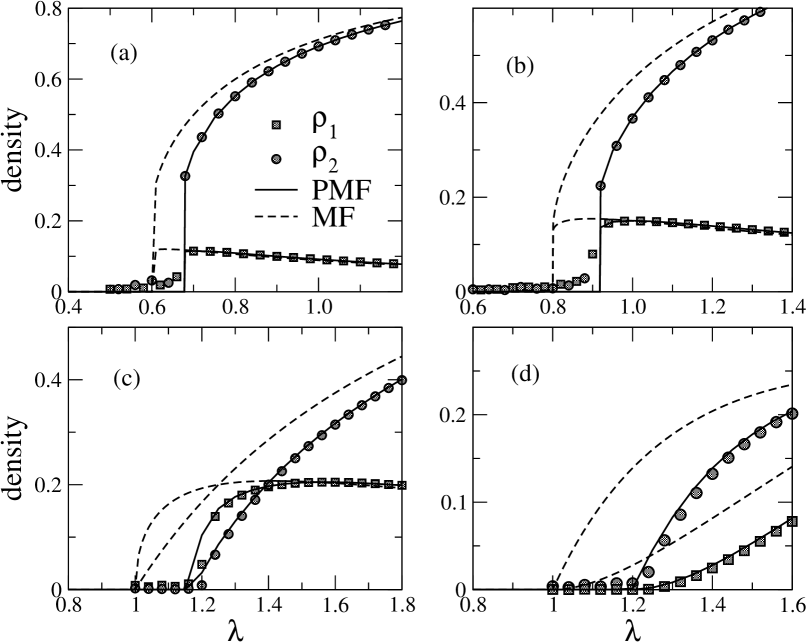
We observe that the ordinary mean-field theory, although qualitatively predicting the discontinuous or continuous nature of the transition, is not quantitatively accurate as indicated by the dashed curves in Fig. 1. However, a far better result is obtained with the PMF theory, represented by the solid curves, presenting an excellent agreement between theory and simulations, for both near and above the transition point regimes irrespective of $\mu$ values. Increasing the connectivity $k$ reduces the transition value of $\lambda$ as can be seen in Table 1. Actually, the threshold will converge to the one-site mean-field value for $k\gg 1$ since this limit corresponds to the fully connected graph for which the one-site theory is exact in the thermodynamical limit.

Figure 2: 2SCP on ER networks with average degree $\langle{k}\rangle=6$. The QS density of single (circles) and doubly (squares) occupied vertices are shown as functions of the infection rate for (a) $\mu=0.1$, (b) $\mu=0.2$, (c) $\mu=0.5$, and (d) $\mu=1$. The dashed curves represent the one-site while solid ones the pairwise mean-field theories. The system size used in simulations is $N=10^{5}$.

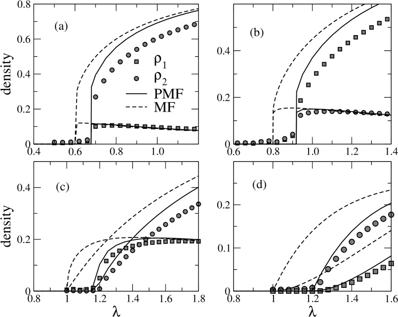
Figure 2 compares the results from simulations and mean field theories for ER networks with $\langle{k}\rangle=6$ using the substitution of $k$ by the mean connectivity $\langle k\rangle$. As observed in RR networks, the one-site approximation reproduces qualitatively well the nature of transition but underestimates the transition point. The PMF accurately matches the transition point and density of singly occupied vertices in the active phase of simulations but underestimates the density of doubly occupied vertices and consequently the overall density of active vertices $\rho=\rho_{1}+\rho_{2}$.

The role of heterogeneity is further investigated in Fig. 3 where the results on BA networks with $\langle k\rangle=10$ are shown. The PMF theory outperforms the ordinary one but still underestimates the location of the phase transition for small values of $\mu$, where the phase transition is discontinuous while yields a very good agreement for the transition point for the continuous cases with $\mu>0.5$ despite of the high heterogeneity of the BA networks, where hubs are expected to play some important role. This finding in the continuous case is in agreement with one-species CP on scale-free networks Muñoz et al. (2010); Ferreira et al. (2011).

Figure 3: 2SCP on BA networks with average degree $\langle{k}\rangle=10$. The QS density of single (circles) and doubly (squares) occupied vertices are shown as functions of the infection rate for (a) $\mu=0.1$, (b) $\mu=0.2$, (c) $\mu=0.5$, and (d) $\mu=1$. The dashed curves represent the one-site while solid ones the pairwise mean-field theories. The system size used in simulations is $N=10^{6}$.

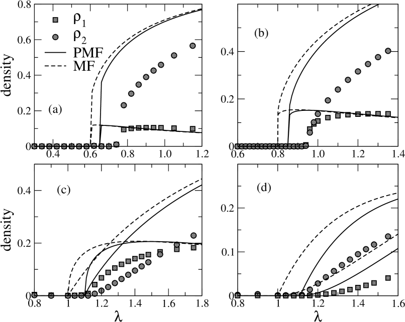
The transition points for the investigated networks (RR, ER and BA) with different average degrees are presented in Table 1. We observe that the PMF theory exhibits a higher accuracy for large average connectivity, as expected, since in the limit $\langle{k}\rangle\gg 1$ corresponds to the fully connected graph where mean-field theories become exact. Another important observation is that the PMF performs worst for BA networks when $\mu$ is small while the accuracy tends to be reduced for larger $\mu$ in RR networks. In BA networks, where hubs are present, small $\mu$ will enhance activity localized in the neighborhood of hubs which, in turn, are not sufficiently mixed for the regime of scale-free networks with $\gamma=3$ Hołyst et al. (2005). More precisely, the star subgraph containing a hub and its nearest-neighbors can stay active in isolation for long periods through a feedback mechanism where the hub activates its neighbors that in turn reactivate the hub recurrently Chatterjee and Durrett (2009); Boguñá et al. (2013); Ferreira et al. (2016). Since localization opposes to the homogeneous mixing hypothesis of the mean-field methods, larger deviations from the theory are indeed expected in this regime. Another intriguing feature of the data of Table 1 is that the PMF thresholds are nearer to the simulations for the slightly heterogeneous ER than from the homogeneous RR networks, which becomes more evident for lower $\langle{k}\rangle$ and higher $\mu$. A similar phenomenon was also observed for the one-species CP on networks Mata et al. (2014) and associated with the approximation $k\approx\langle{k}\rangle$, which would not be observed in a degree-based mean-field theory Pastor-Satorras et al. (2015).

Figure 4: Hysteresis analysis for 2SCP on RR networks with $k=6$ and $\mu=0.2$. Solid curves: PMF theory (arrows indicate the hysteresis flow). Dashed curves: ordinary mean-field theory. Symbols: results from simulations for the RR network with $N=10^{5}$ vertices using different initial conditions.

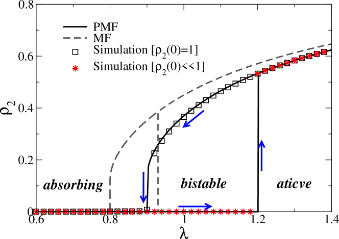
Up to this point, we have addressed the global loss of the stability of the absorbing state that, in the case of discontinuous transitions, involves the transition from an absorbing to a bistable stationary state where both absorbing phase or active phases can be stable depending on the initial condition. We now also consider the loss of global stability of the active phase, i. e., the transition from bistable to active phases. For this aim, we consider an initial condition very close to the absorbing state with a very low density of doubly occupied vertices ($\rho_{1}=0$ and $\rho_{\circ\bullet}\ll 1$) in complement to the fully occupied state $\rho_{\circ\bullet}=1$ used previously. We can, therefore, compute hysteresis curves where the phase coexistence can be derived as in Fig. 4 where one sees absorbing, bistable and active regions.

Figure 5: Phase diagram for the 2SCP obtained from PMF theory for distinct average degree (a) $\langle{k}\rangle=6$, (b) $\langle{k}\rangle=20$, and (d) $\langle{k}\rangle=10^{3}$. Hashed and dotted regions represent bistable and inactive phases respectively while the empty region corresponds to the active phase of PMF theory. Symbols are the results extracted from numerical simulations of different networks models with $N=10^{5}$.

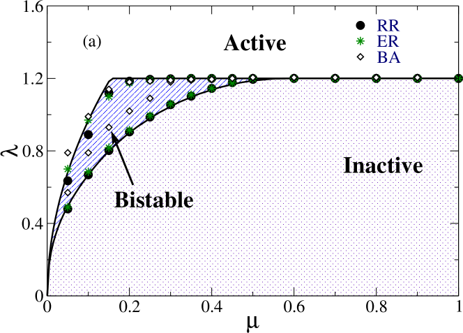
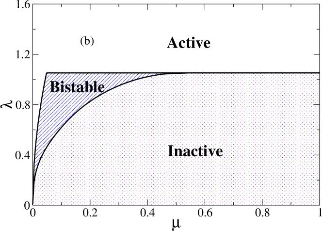
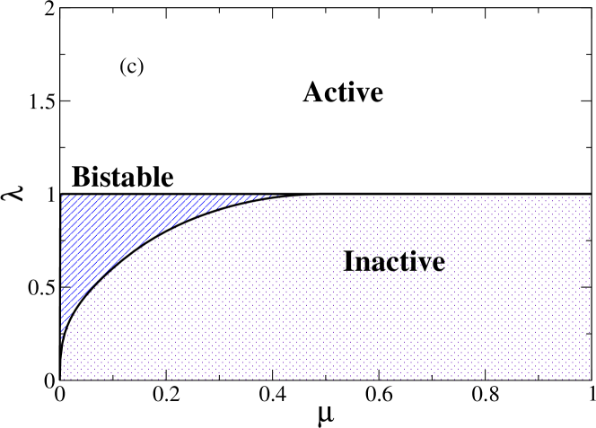
Phase diagrams in the parameter space $(\lambda,\mu)$ obtained via PMF for different connectivities are shown in Fig. 5. The diagrams exhibit three connected regions corresponding to globally inactive (dotted region), globally active (empty region) and bistable (hashed region). An interesting difference with respect to the ordinary mean-field is a transition from a globally stable active phase to a bistable dynamics obtained either by fixing the infection rate $\lambda$ and varying the symbiotic parameter $\mu$ or using fixed $\mu$ and changing $\lambda$ whereas in an ordinary mean-field theory such a transition occurs only for fixed $\mu$; see, for example, Fig. 3 of Ref. Sampaio Filho et al. (2018) which resembles very much the limit of large degree shown in Fig. 5(c). Indeed, the region with double transitions (inactive to bistable and bistable to active) at fixed $\lambda$, occurring in the small $\mu$ region, shrinks as the connectivity increases towards a fully connected graph limit as shown in Figs. 5(b) and (c). Triple points shown in the phase diagrams depend on connectivity, departing from $(\lambda_{\text{t}},\mu_{\text{t}})=(1,1/2)$ for the complete graph (one-site mean-field) De Oliveira et al. (2012) to $\lambda_{\text{t}}=\tfrac{\langle{k}\rangle}{\langle{k}\rangle-1}$ and $\mu_{\text{t}}=0.501(1),~{}0.545(5)$, and $0.595(5)$ for $\langle{k}\rangle=10^{3}$, $20$, and $6$, respectively. It worths to comment that phase diagrams with qualitatively similar spinoidals found in 2SCP with our PMF theory have been reported for other models with abrupt transitions on networks Maj (2014); Böttcher et al. (2017a, a); Valdez et al. (2016) with a difference that they were obtained by a first-order mean-field theory, whereas in the 2SCP model we needed to go up to a second-order pairwise theory.

Figure 5(a) also presents the phase diagram obtained via simulations on different graphs with average degree $\langle{k}\rangle=6$. One observes a remarkable good match between simulations and theory for RR and ER (homogeneous) networks. The quantitative agreement is less satisfactory for BA model, but it is still qualitatively correct. The dynamical correlations in these infinite dimensional systems have proven to lead not just to a quantitatively better theory but also to new behaviors not predicted by the ordinary mean-field theory.

VI Conclusions

Stochastic interacting systems with cooperative or synergistic couplings can be used for modeling different phenomena, such as coinfections of pathological agents, social relations, and ecological interactions, among others. One key issue of these models involves the nonequilibrium phase transitions among active and absorbing phases that can emerge in some systems, especially the abrupt ones, where macroscopic order parameters change discontinuously. Moreover, understanding the behavior of these transitions taking place on the top of complex networks has become very relevant since most of these dynamical processes indeed involve interactions mediated by networked systems. In the present work we investigate a simple model, in which two species lying on networks interact symbiotically, the symbiotic contact process De Oliveira et al. (2012). We used both stochastic simulations and mean-field pairwise approximations, the latter reckoning dynamical correlations not considered in previous analytical (one-site mean-field) studies of this model.

The PMF theory outperforms the ordinary one and, more importantly, predicts features not captured by the latter, in agreement with the simulations on distinct types of networks with homogeneous, Poissonian, and scale-free degree distributions. In the case of homogeneous networks, the PMF theory is accurate describing very well both the dynamics near and above the transitions (supercritical region). Despite of disregarding the heterogeneity of the networks, our theory also gives very good estimates of the transition points in the case of Poissonian and scale-free networks but cannot quantitatively capture the prevalence in the highly active regime.

We also investigated the phase diagrams exhibiting globally absorbing, bistable, and globally active regions. The PMF theory, beyond being quantitatively more accurate than the ordinary one, provides a much richer phase diagram where discontinuous transitions, involving bistable phases, can be obtained either varying the infection rate $\lambda$ or the symbiosis parameter $\mu$ independently, whereas this transition happens only at fixed $\mu$ in the one-site approach. These PMF results are confirmed by extensive numerical simulations. Our findings provide an important example of the role played by dynamical correlations in cooperative processes on networked substrates, which is commonly not considered in other theoretical approaches. Pair-approximations as the one developed in this work can be used to improve the accuracy of phase diagrams observed in other related works Maj (2014); Böttcher et al. (2017b) where first order mean-field theory captures the qualitative behavior but analytical spinoidals deviate from simulations when the average connectivity is reduced. Finally, we expect that our work will stimulate future analysis of dynamical correlations on other cooperative processes.

The theories presented in this paper do not include the network heterogeneity and, specially, the degree distribution. As a prospect for forthcoming analysis, one could use degree-based Pastor-Satorras et al. (2015) or individual-based Van Mieghem (2012) mean-field theories to tackle the role of heterogeneity.

Appendix A Pair mean-field theory

In the pair approximation, the seven two-site variables to be considered are $[\circ,\bullet]$, $[\circ,\circ]$ $[\times,\circ]$, $[\circ,{\circ\bullet}]$, $[{\circ\bullet},{\circ\bullet}]$, $[\times,{\circ\bullet}]$, and $[\times,\times]$. All other combinations are equivalent to some of them, due to symmetry. Considering that every vertex has $k$ nearest-neighbors, after some algebra we obtain the following set of dynamical equations

$$\frac{d[\circ,\bullet]}{dt} = -2(1+{\lambda}/{k})[\circ,\bullet]+2\mu[\circ,{\circ\bullet}]+2\lambda\frac{k-1}{k}([\circ,\times,\bullet]+[\circ,\times,{\circ\bullet}]-[\circ,\bullet,\circ]-[\circ,\bullet,{\circ\bullet}])$$ (13)

$$\frac{d[\circ,{\circ\bullet}]}{dt} = -(1+2\mu+\lambda/k)[\circ,{\circ\bullet}]+\mu[{\circ\bullet},{\circ\bullet}]+\frac{\lambda}{k}([\circ,\bullet]+[\times,{\circ\bullet}])+$$ (14)

$$+\lambda\frac{k-1}{k}([\circ,\times,{\circ\bullet}]+[{\circ\bullet},\times,{\circ\bullet}]+[\circ,\circ,\bullet]+[\circ,\circ,{\circ\bullet}]+[\circ,\bullet,\circ]-[{\circ\bullet},\circ,{\circ\bullet}]).$$

$$\frac{d[\times,\times]}{dt} = 4[\circ,\times]-4\lambda\frac{k-1}{k}([\times,\times,\circ]+[\times,\times,{\circ\bullet}])$$ (15)

$$\frac{d[\circ,\circ]}{dt} = 2(-[\circ,\circ]+\mu[\circ,{\circ\bullet}]+\frac{\lambda}{k}[\circ,\times])+2\lambda\frac{k-1}{k}([\circ,\times,\circ]+[\circ,\times,{\circ\bullet}]-[\circ,\circ,\bullet]-[\circ,\circ,{\circ\bullet}]).$$ (16)

$$\frac{d[{\circ\bullet},{\circ\bullet}]}{dt} = -4[{\circ\bullet},{\circ\bullet}]+4\frac{\lambda}{k}[\circ,{\circ\bullet}]+4\lambda\frac{k-1}{k}([{\circ\bullet},\circ,{\circ\bullet}]+[{\circ\bullet},\circ,\bullet])$$ (17)

$$\frac{d[\circ,\times]}{dt} = -[\circ,\times]-\frac{\lambda}{k}[\circ,\times]+\mu[{\circ\bullet},\times]+[\circ,\circ]+[\circ,\bullet]+$$ (18)

$$+\lambda\frac{k-1}{k}([\circ,{\times,\times}]+[{\circ\bullet},{\times,\times}]-[{\circ,\times},\circ]-2[{\circ,\times},{\circ\bullet}]-[{\circ,\times},\bullet]-[\bullet,{\circ,\times}]-[{\circ\bullet},{\circ,\times}]).$$

$$\frac{d[{\circ\bullet},\times]}{dt} = -2(\mu+\lambda/k)[{\circ\bullet},\times]+2[{\circ\bullet},\circ]+2\lambda\frac{k-1}{k}([\circ,\bullet,\times]+[{\circ\bullet},{\circ,\times}]-[{\circ\bullet},\times,\circ]-[{\circ\bullet},\times,{\circ\bullet}]).$$ (19)

Let us explain in details the terms in Eq. (13). The derivation of the remaining equations follows from a similar reasoning. Thus, in Eq. (13), the term proportional to $[\circ,\bullet]$ represents two contributions. The one proportional to $-2$ is the spontaneous annihilation of each individual ($\circ\to\times$ and $\bullet\to\times$). The term proportional to $2\lambda/k$ represents the creation of each individual of this pair into the other ($\circ,\bullet\to{\circ\bullet},\bullet$ and $\circ,\bullet\to\circ,{\circ\bullet}$). The term proportional to $[\circ,{\circ\bullet}]$ is due to the annihilation with rate $\mu$ of each individual in the doubly occupied vertex (${\circ\bullet}\to\circ$ and ${\circ\bullet}\to\bullet$). Finally, the triplet terms represent the creation of outsiders into the pair. For example, the first triplet term represents the transition $\circ,\times\to\circ,\bullet$ due to A ($\circ$) individuals in each remaining $k-1$ neighbors of the empty vertex ($\times$), while the factor 2 comes from the transition $\times,\bullet\to\circ,\bullet$ of B ($\bullet$) individuals neighboring the empty vertex. The remaining triplets terms can be rationalized in the same way.

We now proceed with the pair approximations, $[S,S^{\prime},S^{\prime\prime}]=\frac{[S,S^{\prime}][S^{\prime},S^{\prime\prime}]}{[S^{\prime}]}$ in Eqs. (13) to (19), and find that them can be approximated as

$$\frac{d[\circ,\bullet]}{dt} = -2(1+{\lambda}/{k})[\circ,\bullet]+2\mu[\circ,{\circ\bullet}]+2\lambda\frac{k-1}{k}\left(\frac{[\circ,\times]^{2}+[\circ,\times][\times,{\circ\bullet}]}{[\times]}-\frac{[\circ,\bullet]^{2}+[\circ,\bullet][\bullet,{\circ\bullet}]}{[\bullet]}\right)$$ (20)

$$\frac{d[\circ,{\circ\bullet}]}{dt} = -(1+2\mu+\lambda/k)[\circ,{\circ\bullet}]+\mu[{\circ\bullet},{\circ\bullet}]+\frac{\lambda}{k}([\circ,\bullet]+[\times,{\circ\bullet}])+$$ (22)

$$+\lambda\frac{k-1}{k}\left(\frac{[\circ,\times]+[\times,{\circ\bullet}]}{[\times]}[\times,{\circ\bullet}]+\frac{[\circ,\circ]([\circ,\bullet]+[\circ,{\circ\bullet}])+[\circ,\bullet]^{2}-[\circ,{\circ\bullet}]^{2}}{[\circ]}\right).$$

$$\frac{d[\times,\times]}{dt} = 4[\circ,\times]-4\lambda\frac{k-1}{k}\frac{[\times,\times]}{[\times]}([\times,\circ]+[\times,{\circ\bullet}])$$ (23)

$$\frac{d[\circ,\circ]}{dt} = 2(-[\circ,\circ]+\mu[\circ,{\circ\bullet}]+\frac{\lambda}{k}[\circ,\times])+2\lambda\frac{k-1}{k}\left(\frac{[\circ,\times]+[\times,{\circ\bullet}]}{[\times]}[\circ,\times]-\frac{[\circ,\bullet]+[\circ,{\circ\bullet}]}{[\circ]}[\circ,\circ]\right).$$ (24)

$$\frac{d[{\circ\bullet},{\circ\bullet}]}{dt} = -4[{\circ\bullet},{\circ\bullet}]+4\frac{\lambda}{k}[\circ,{\circ\bullet}]+4\lambda\frac{k-1}{k}\frac{[{\circ\bullet},\circ]}{[\circ]}\left([\circ,{\circ\bullet}]+[\circ,\bullet]\right)$$ (25)

$$\frac{d[\circ,\times]}{dt} = -\left(1+\frac{\lambda}{k}\right)[\circ,\times]+\mu[{\circ\bullet},\times]+[\circ,\circ]+[\circ,\bullet]+\lambda\frac{k-1}{k}\times$$ (26)

$$\left(\frac{([\circ,\times]+[{\circ\bullet},\times])([\times,\times]+2[\circ,\times]}{[\times]}-\frac{[\bullet,\circ]+[{\circ\bullet},\circ]}{[\circ]}[\circ,\times]\right)$$

$$\frac{d][{\circ\bullet},\times]}{dt} = -2(\mu+\lambda/k)[{\circ\bullet},\times]+2[{\circ\bullet},\circ]+2\lambda\frac{k-1}{k}\left(\frac{[\circ,\bullet]+[{\circ\bullet},\circ]}{[\circ]}[\circ,\times]-\frac{[\times,\circ]+[\times,{\circ\bullet}]}{[\times]}[{\circ\bullet},\times]\right).$$ (27)

References

- D’Souza et al. (2019) R. M. D’Souza, J. Gómez-Gardeñes, J. Nagler, and A. Arenas, “Explosive Phenomena in Complex Networks,” Adv. Phys. 68, 123 (2019).
- Perc et al. (2017) M. Perc, J. J. Jordan, D. G. Rand, Z. Wang, S. Boccaletti, and A. Szolnoki, “Statistical physics of human cooperation,” Phys. Rep. 687, 1 (2017).
- Gómez-Gardeñes et al. (2016) J. Gómez-Gardeñes, L. Lotero, S. N. Taraskin, and F. J. Pérez-Reche, “Explosive Contagion in Networks,” Sci. Rep. 6, 19767 (2016).
- Wang et al. (2019) W. Wang, Q.-H. Liu, J. Liang, Y. Hu, and T. Zhou, “Coevolution spreading in complex networks,” Phys. Rep. (2019).
- Cai et al. (2015) W. Cai, L. Chen, F. Ghanbarnejad, and P. Grassberger, “Avalanche outbreaks emerging in cooperative contagions,” Nat. Phys. 11, 936 (2015).
- Grassberger et al. (2016) P. Grassberger, L. Chen, F. Ghanbarnejad, and W. Cai, “Phase transitions in cooperative coinfections: Simulation results for networks and lattices,” Phys. Rev. E 93, 042316 (2016).
- Boccaletti et al. (2016) S. Boccaletti, J. Almendral, S. Guan, I. Leyva, Z. Liu, I. Sendiña-Nadal, Z. Wang, and Y. Zou, “Explosive transitions in complex networks’ structure and dynamics: Percolation and synchronization,” Phys. Rep. 660, 1 (2016).
- Albert and Barabási (2002) R. Albert and A.-L. Barabási, “Statistical mechanics of complex networks,” Rev. Mod. Phys. 74, 47 (2002).
- Pastor-Satorras et al. (2015) R. Pastor-Satorras, C. Castellano, P. Van Mieghem, and A. Vespignani, “Epidemic processes in complex networks,” Rev. Mod. Phys. 87, 925 (2015).
- Castellano et al. (2009) C. Castellano, S. Fortunato, and V. Loreto, “Statistical physics of social dynamics,” Rev. Mod. Phys. 81, 591 (2009).
- Ohtsuki et al. (2006) H. Ohtsuki, C. Hauert, E. Lieberman, and M. A. Nowak, “A simple rule for the evolution of cooperation on graphs and social networks,” Nature 441, 502 (2006).
- Strogatz (2018) S. H. Strogatz, Nonlinear Dynamics and Chaos (CRC Press, 2018).
- Newman (2005) M. E. J. Newman, “Threshold Effects for Two Pathogens Spreading on a Network,” Phys. Rev. Lett. 95, 108701 (2005).
- Newman and Ferrario (2013) M. E. J. Newman and C. R. Ferrario, “Interacting Epidemics and Coinfection on Contact Networks,” PLoS One 8, e71321 (2013).
- Chen et al. (2013) L. Chen, F. Ghanbarnejad, W. Cai, and P. Grassberger, “Outbreaks of coinfections: The critical role of cooperativity,” EPL (Europhysics Lett. 104, 50001 (2013).
- Janssen and Stenull (2016) H.-K. Janssen and O. Stenull, “First-order phase transitions in outbreaks of co-infectious diseases and the extended general epidemic process,” EPL (Europhysics Lett. 113, 26005 (2016).
- Cui et al. (2017) P.-B. Cui, F. Colaiori, and C. Castellano, “Mutually cooperative epidemics on power-law networks,” Phys. Rev. E 96, 022301 (2017).
- Liu et al. (2017) Q. Liu, W. Wang, M. Tang, T. Zhou, and Y. Lai, “Explosive spreading on complex networks: The role of synergy,” Phys. Rev. E 95, 042320 (2017).
- Tubay et al. (2013) J. M. Tubay, H. Ito, T. Uehara, S. Kakishima, S. Morita, T. Togashi, K. Tainaka, M. P. Niraula, B. E. Casareto, Y. Suzuki, and J. Yoshimura, “The paradox of enrichment in phytoplankton by induced competitive interactions,” Sci. Rep. 3, 2835 (2013).
- Dobramysl and Täuber (2013) U. Dobramysl and U. C. Täuber, “Environmental versus demographic variability in two-species predator-prey models,” Phys. Rev. Lett. 110, 048105 (2013).
- Court et al. (2013) S. J. Court, R. A. Blythe, and R. J. Allen, “Parasites on parasites: Coupled fluctuations in stacked contact processes,” EPL (Europhysics Lett. 101, 50001 (2013).
- Markham et al. (2013) D. C. Markham, M. J. Simpson, P. K. Maini, E. A. Gaffney, and R. E. Baker, “Incorporating spatial correlations into multispecies mean-field models,” Phys. Rev. E 88, 052713 (2013).
- Iwata et al. (2011) S. Iwata, K. Kobayashi, S. Higa, J. Yoshimura, and K. ichi Tainaka, “A simple population theory for mutualism by the use of lattice gas model,” Ecol. Modell. 222, 2042 (2011).
- De Oliveira et al. (2012) M. M. De Oliveira, R. V. Dos Santos, and R. Dickman, “Symbiotic two-species contact process,” Phys. Rev. E 86 (2012).
- Harris (1974) T. E. Harris, “Contact Interactions on a Lattice,” Ann. Probab. 2, 969 (1974).
- Castellano and Pastor-Satorras (2006) C. Castellano and R. Pastor-Satorras, “Non-Mean-Field Behavior of the Contact Process on Scale-Free Networks,” Phys. Rev. Lett. 96, 038701 (2006).
- Ferreira et al. (2011) S. C. Ferreira, R. S. Ferreira, C. Castellano, and R. Pastor-Satorras, “Quasistationary simulations of the contact process on quenched networks,” Phys. Rev. E 84, 066102 (2011).
- Marro and Dickman (2005) J. Marro and R. Dickman, Nonequilibrium Phase Transitions in Lattice Models, Aléa-Saclay (Cambridge University Press, 2005).
- de Oliveira and Dickman (2014) M. M. de Oliveira and R. Dickman, “Phase diagram of the symbiotic two-species contact process,” Phys. Rev. E 90, 032120 (2014).
- Sampaio Filho et al. (2018) C. I. N. Sampaio Filho, T. B. dos Santos, N. A. M. Araújo, H. A. Carmona, A. A. Moreira, and J. S. Andrade, “Symbiotic contact process: Phase transitions, hysteresis cycles, and bistability,” Phys. Rev. E 98, 062108 (2018).
- Barabási and Pósfai (2016) A.-L. Barabási and M. Pósfai, Network science (Cambridge University Press, Cambridge, 2016).
- Gleeson (2011) J. P. Gleeson, “High-Accuracy Approximation of Binary-State Dynamics on Networks,” Phys. Rev. Lett. 107, 068701 (2011).
- Ben-Avraham and Köhler (1992) D. Ben-Avraham and J. Köhler, “Mean-field (n,m)-cluster approximation for lattice models,” Phys. Rev. A 45, 8358 (1992).
- Keeling (1999) M. J. Keeling, “The effects of local spatial structure on epidemiological invasions,” Proc. R. Soc. London. Ser. B Biol. Sci. 266, 859 (1999).
- Eames and Keeling (2002) K. T. D. Eames and M. J. Keeling, “Modeling dynamic and network heterogeneities in the spread of sexually transmitted diseases,” Proc. Natl. Acad. Sci. 99, 13330 (2002).
- Gleeson (2013) J. P. Gleeson, “Binary-State Dynamics on Complex Networks: Pair Approximation and Beyond,” Phys. Rev. X 3, 021004 (2013).
- Mata et al. (2014) A. S. Mata, R. S. Ferreira, and S. C. Ferreira, “Heterogeneous pair-approximation for the contact process on complex networks,” New J. Phys. 16, 053006 (2014).
- Barabási and Albert (1999) A. L. Barabási and R. Albert, “Emergence of scaling in random networks,” Science 286, 509 (1999).
- Ferreira and Ferreira (2013) R. S. Ferreira and S. C. Ferreira, “Critical behavior of the contact process on small-world networks,” Eur. Phys. J. B 86, 462 (2013).
- Catanzaro et al. (2005) M. Catanzaro, M. Boguñá, and R. Pastor-Satorras, “Generation of uncorrelated random scale-free networks,” Phys. Rev. E 71, 027103 (2005).
- Muñoz et al. (2010) M. A. Muñoz, R. Juhász, C. Castellano, and G. Ódor, “Griffiths Phases on Complex Networks,” Phys. Rev. Lett. 105, 128701 (2010).
- Watts and Strogatz (1998) D. J. Watts and S. H. Strogatz, “Collective dynamics of ‘small-world’ networks,” Nature 393, 440 (1998).
- Cota and Ferreira (2017) W. Cota and S. C. Ferreira, “Optimized Gillespie algorithms for the simulation of Markovian epidemic processes on large and heterogeneous networks,” Comput. Phys. Commun. 219, 303 (2017).
- De Oliveira and Dickman (2005) M. M. De Oliveira and R. Dickman, “How to simulate the quasistationary state,” Phys. Rev. E 71, 016129 (2005).
- Ferreira et al. (2016) S. C. Ferreira, R. S. Sander, and R. Pastor-Satorras, “Collective versus hub activation of epidemic phases on networks,” Phys. Rev. E 93, 032314 (2016).
- de Arruda et al. (2017) G. F. de Arruda, E. Cozzo, T. P. Peixoto, F. A. Rodrigues, and Y. Moreno, “Disease Localization in Multilayer Networks,” Phys. Rev. X 7, 011014 (2017).
- Valdano et al. (2015) E. Valdano, L. Ferreri, C. Poletto, and V. Colizza, “Analytical Computation of the Epidemic Threshold on Temporal Networks,” Phys. Rev. X 5, 021005 (2015).
- Sander et al. (2016) R. S. Sander, G. S. Costa, and S. C. Ferreira, “Sampling methods for the quasistationary regime of epidemic processes on regular and complex networks,” Phys. Rev. E 94, 042308 (2016).
- Hołyst et al. (2005) J. A. Hołyst, J. Sienkiewicz, A. Fronczak, P. Fronczak, and K. Suchecki, “Universal scaling of distances in complex networks,” Phys. Rev. E 72, 026108 (2005).
- Chatterjee and Durrett (2009) S. Chatterjee and R. Durrett, “Contact processes on random graphs with power law degree distributions have critical value 0,” Ann. Probab. 37, 2332 (2009).
- Boguñá et al. (2013) M. Boguñá, C. Castellano, and R. Pastor-Satorras, “Nature of the Epidemic Threshold for the Susceptible-Infected-Susceptible Dynamics in Networks,” Phys. Rev. Lett. 111, 068701 (2013).
- Maj (2014) “Spontaneous recovery in dynamical networks,” Nat. Phys. 10, 34 (2014).
- Böttcher et al. (2017a) L. Böttcher, J. Nagler, and H. J. Herrmann, “Critical Behaviors in Contagion Dynamics,” Phys. Rev. Lett. 118, 088301 (2017a).
- Valdez et al. (2016) L. D. Valdez, M. A. Di Muro, and L. A. Braunstein, “Failure-recovery model with competition between failures in complex networks: a dynamical approach,” J. Stat. Mech. Theory Exp. 2016, 093402 (2016).
- Böttcher et al. (2017b) L. Böttcher, M. Luković, J. Nagler, S. Havlin, and H. J. Herrmann, “Failure and recovery in dynamical networks,” Sci. Rep. 7, 41729 (2017b).
- Van Mieghem (2012) P. Van Mieghem, “Epidemic phase transition of the SIS type in networks,” EPL (Europhysics Lett. 97, 48004 (2012).