Quantum steering of Bell-diagonal states with generalized measurements

Abstract

The phenomenon of quantum steering in bipartite quantum systems can be reduced to the question whether or not the first party can perform measurements such that the conditional states on the second party can be explained by a local hidden state model. Clearly, the answer to this depends on the measurements which the first party is able to perform. We introduce a local hidden state model explaining the conditional states for all generalized measurements on Bell-diagonal states of two qubits. More precisely, it is known for the restricted case of projective measurements and Bell-diagonal states characterised by the correlation matrix $T$ that a local hidden state model exists if and only if $R_{T}=2\pi N_{T}\left|\det(T)\right|\geq 1$, where $N_{T}$ is defined by an integral over the Bloch sphere. For generalized measurements described by positive operator valued measures we construct a model if $R_{T}\geq 6/5$. Our work paves the way for a systematic study of steerability of quantum states with generalized measurements beyond the highly-symmetric Werner states.

I Introduction

Since its first description in 1935, the Einstein-Podolsky-Rosen (EPR) argument Einstein et al. (1935); Einstein (1948) has been at the center of many debates on the foundations of quantum mechanics and, at the same time, also a welling source of inspiration. Pondering on it, Bell introduced the concept of nonlocality Bell (1964); reconsidering the issue later, Werner and Primas defined modern notions of classical correlations and entanglement Primas ; Werner ; Werner (1989). Both the theory of Bell nonlocality and of entanglement have played a crucial role in the development of modern quantum information theory. Based on ideas of Schrödinger, Wiseman and collaborators showed more recently that behind the EPR argument is yet another concept of quantum nonlocality, called quantum steering Wiseman et al. (2007); Schrödinger (1935). This discovery since then has caused a new surge of research in quantum information theory. Characterization of quantum steering has been studied, many connections to different areas of quantum information were found and applications were established, for a recent review see Ref. Uola et al. (2019).

For explaining the notion of quantum steering, suppose Alice and Bob share a bipartite quantum state $\rho$ over the finite-dimensional Hilbert space $\mathcal{H}_{A}\otimes\mathcal{H}_{B}$ and Alice performs measurements on her side. The most general measurement with $n$ outcomes is described by a positive operator valued measure ($n$-POVM). Such a measure $E$ is a collection of $n$ positive operators, $E=\{E_{i}\}_{i=1}^{n}$, $E_{i}\geq 0$, fulfilling the normalization $\sum_{i=1}^{n}E_{i}=\openone_{A}$, where $\openone_{A}$ is the identity operator on $\mathcal{H}_{A}$ (similarly, $\openone_{B}$ will denote the identity operator acting on $\mathcal{H}_{B}$).

After Alice performed the measurement and obtained the result, Bob’s resulting states form the steering ensemble of conditional states, $\{\operatorname{Tr}_{A}[\rho(E_{i}\otimes\openone_{B})]\}_{i=1}^{n}$. If, however, the entanglement between the two parties is not sufficiently strong, the conditional states can be locally simulated by a so-called local hidden state model Wiseman et al. (2007). The strategy of simulating goes as follows. Alice, instead of providing Bob with a part of the entangled state, simply sends him an ensemble of states $\{\sigma_{\lambda}\}$ indexed by some variable $\lambda$ distributed according to a distribution $p(\lambda)$, known as local hidden states (LHS).

To simulate the steering corresponding to measurement $\{E_{i}\}_{i=1}^{n}$, Alice assigns state $\sigma_{\lambda}$ to outcome $i$ according to certain designed probability $G_{i}(\lambda)$. The functions $G=\{G_{i}\}_{i=1}^{n}$, thus satisfying $G_{i}(\lambda)\geq 0$ and $\sum_{i=1}^{n}G_{i}(\lambda)=1$ for each $\lambda$, are referred to as response functions. In this way Alice can simulate the steering ensemble by averaging over states associated to each outcome,

$$\operatorname{Tr}_{A}[\rho(E_{i}\otimes\openone_{B})]=\sum_{\lambda}G_{i}(\lambda)p(\lambda)\sigma_{\lambda}.$$ (1)

Here the summation can be reformulated as an integration over an appropriate measure if required. Eq. (1) ensures that Bob, when performing state tomography conditioned on Alice’s outcomes, obtains the same result as if Alice were steering his system by means of measurement $E$ Wiseman et al. (2007). If the design of the LHS ensemble $\{\sigma_{\lambda}\}$ is such that for all measurements $E$ Alice can find a response function $G$ such that Eq. (1) holds, we say that the state is unsteerable; otherwise it is steerable.

This definition also extends naturally to the case where Alice is limited to certain subsets of measurements. Most often she is limited to performing projective measurements (or projector values measures, PVMs) only. In this case, for certain important entangled states LHS models exist, proving the states to be unsteerable Wiseman et al. (2007). Some of these models can also be shown to be optimal, leading to an exact characterization of steering in these cases. These include the Werner states Werner (1989); Wiseman et al. (2007), the isotropic states Wiseman et al. (2007) or general two-qubit states Nguyen et al. (2019), where the solution for Bell-diagonal states is particularly simple Jevtic et al. (2015); Nguyen and Vu (2016a, b). If the most general measurements in quantum mechanics are taken into account, namely those described by general POVMs, the construction of LHS models is difficult. The most important known model is arguably the Barrett model, which was constructed for Werner states and isotropic states Barrett (2002). Contrary to the models for projective measurements, Barrett’s model has never been demonstrated to be optimal; in fact evidence indicates that it is not Nguyen et al. (2018, 2019). Barrett’s model also appeared to be ad hoc, seemingly limited to only Werner states and isotropic states, which are highly symmetric.

In this work, we generalize the Barrett construction of an LHS model to a more general family of two-qubit states, those which can be considered as a mixture of Bell states, or Bell-diagonal states. Quantum steering of Bell-diagonal states when measurements are limited to projective measurements has been recently understood Jevtic et al. (2015); Nguyen and Vu (2016a, b). With our new LHS model for POVMs we can prove the unsteerability of a significant set of Bell-diagonal states. Our model is one of the first LHS models for POVMs on two-qubit states beyond the highly symmetric cases. In fact there is, to our knowledge, only one other LHS model for POVMs, which is based on LHS models for projective measurements Hirsch et al. (2013). The model is, however, more limited and paradoxically appears to be more effective only for high-dimensional system rather than for two-qubit states. In our work we also explicitly demonstrate that our construction is still non-optimal, as it fails to detect the unsteerability of some separable Bell-diagonal states.

In the following, we start with introducing the Bloch four-vector representation of operators acting on qubit systems. After recalling the known results on quantum steering of Bell-diagonal states, we will describe the construction of our LHS model for POVMs.

II Bloch representation and Bell-diagonal states

For a qubit, any operator $X$ can be conveniently presented by a four-vector, ${x_{0}}\choose{\boldsymbol{x}}$, referred to as the Bloch representation. This is defined according to the expansion

$$X=\frac{1}{2}\sum_{i=0}^{3}x_{i}\sigma_{i},$$ (2)

where $\sigma_{k}$ for $k=0,1,2,3$ are the Pauli matrices extended to also include the identity matrix. In particular, projections or pure states are represented by ${1}\choose{\boldsymbol{n}}$, with $\boldsymbol{n}$ being an unit vector. The set of pure states is thus a sphere, known as the Bloch sphere. Similarly, a two-qubit state $\rho$ can be most conveniently characterized by its Bloch tensor,

$$\rho=\frac{1}{4}\sum_{i,j=0}^{3}\Lambda_{ij}\sigma_{i}\otimes\sigma_{j}.$$ (3)

The states that are diagonal in the Bell basis are those for which Alice’s and Bob’s reduced states are maximally mixed Horodecki and Horodecki (1996). The Bloch tensor $\Lambda$ can thus be written as

$$\Lambda=\begin{pmatrix}1&0\\ 0&T\end{pmatrix},$$ (4)

where $T$ is s $(3\times 3)$ matrix representing the correlation between them. Without loss of generality, we can assume that $T$ is diagonal. The reason is that the steering properties of a quantum state are invariant under local unitary transformations acting on the states. These transformations act as orthogonal transformations on the matrix $T$, and due to the singular value decomposition this can be used to diagonalize $T$ Horodecki and Horodecki (1996).

III Steering with projective measurements

To explain our construction, we first recall the optimal LHS model for Bell-diagonal states if measurements are limited to projective ones Jevtic et al. (2015); Nguyen and Vu (2016a, b). A projective measurement on Alice’s side corresponds to a pair of effects, which can be represented by Bloch vectors ${1}\choose{\boldsymbol{e}_{1}}$ and $1\choose\boldsymbol{e}_{2}$ with two unit vectors $\boldsymbol{e}_{2}=-\boldsymbol{e}_{1}$. As Alice gets outcomes $i\in\{1,2\}$, a direct calculation shows that Bob’s conditional states are

$$\frac{1}{2}\begin{pmatrix}1\\ T\boldsymbol{e}_{i}\end{pmatrix},$$ (5)

where we have used the fact that $T$ is symmetric, $T^{T}=T$.

Recall that the optimal ensemble of hidden states for a Bell-diagonal state is defined by the following distribution on Bob’s Bloch sphere Jevtic et al. (2015); Nguyen and Vu (2016a)

$$p_{J}(\boldsymbol{n})=\frac{N_{T}}{[\boldsymbol{n}^{T}T^{-2}\boldsymbol{n}]^{2}},$$ (6)

where $N_{T}$ is the normalization factor, given by

$$N_{T}^{-1}=\int\mathrm{d}S(\boldsymbol{n})\frac{1}{[\boldsymbol{n}^{T}T^{-2}\boldsymbol{n}]^{2}},$$ (7)

where the integral is taken over the surface of the Bloch sphere with $\mathrm{d}S$ being the surface measure. The response function for projective measurements is chosen as Jevtic et al. (2015)

$$G^{J}_{i}(\boldsymbol{n})=\Theta(\boldsymbol{e}^{T}_{i}T^{-1}\boldsymbol{n}),$$ (8)

where $\Theta$ is the Heaviside step function.

The conditional states produced by this LHS model can be computed to be

$$\int\mathrm{d}S(\boldsymbol{n})\frac{N_{T}}{[\boldsymbol{n}^{T}T^{-2}\boldsymbol{n}]^{2}}\Theta(\boldsymbol{e}^{T}_{i}T^{-1}\boldsymbol{n})\begin{pmatrix}1\\ \boldsymbol{n}\end{pmatrix}=\frac{1}{2}\begin{pmatrix}1\\ R_{T}T\boldsymbol{e}_{i}\end{pmatrix},$$ (9)

where

$$R_{T}=2\pi N_{T}\left|\det(T)\right|.$$ (10)

Comparing this with the conditional states due to the actual measurements at Alice’s side in Eq. (5), one sees that $R_{T}\geq 1$ suffices to deduce that the corresponding Bell-diagonal state is unsteerable Jevtic et al. (2014, 2015): If $R_{T}=1$ the LHS model simulates exactly the state, while for $R_{T}>1$ the LHS model allows even to simulate a state with stronger correlations.

The described construction of the LHS ensemble was later proven to be optimal Nguyen and Vu (2016a, b), thus this is also a necessary condition for the Bell-diagonal state to be unsteerable. In fact, the quantity $R_{T}$ has been generalized for general states, where it is referred to as the critical radius of the state Nguyen et al. (2018).

IV Steering with positive operator valued measures

We now consider the case where Alice makes a POVM. It is known that in studying steerability of qubits, it is sufficient to consider POVMs consisting of four rank-$1$ effects, as these are the extremal POVMs Barrett (2002); D’Ariano et al. (2005). A range-$1$ POVM of $4$ outcomes is given by effects $\alpha_{i}{{1}\choose{\boldsymbol{e}_{i}}}$ with $0\leq\alpha_{i}\leq 1$ such that

$$\sum_{i=1}^{4}\alpha_{i}\begin{pmatrix}1\\ \boldsymbol{e}_{i}\end{pmatrix}=\begin{pmatrix}2\\ \boldsymbol{0}\end{pmatrix},$$ (11)

where one should recall that $2\choose\boldsymbol{0}$ represents the identity operator. Corresponding to the measurement outcome $i$, the conditional state on Bob’s side is

$$\frac{\alpha_{i}}{2}\begin{pmatrix}1\\ T\boldsymbol{e}_{i}\end{pmatrix}.$$ (12)

Our purpose is to construct a possible LHS model to model these conditional ensembles of states. The probability distribution of the LHS ensemble is still defined by Eq. (6). To define the response function, we first denote

$$g_{i}(\boldsymbol{n})=\frac{1}{2}\left(1+\frac{\boldsymbol{e}_{i}^{T}T^{-1}\boldsymbol{n}}{\left\|T^{-1}\boldsymbol{n}\right\|}\right)\Theta(\boldsymbol{e}^{T}_{i}T^{-1}\boldsymbol{n}),$$ (13)

and

$$c_{i}=\int\mathrm{d}S(\boldsymbol{n})p_{J}(\boldsymbol{n})g_{i}(\boldsymbol{n}).$$ (14)

Note that

$$0\leq c_{i}\leq\int\mathrm{d}S(\boldsymbol{n})p_{J}(\boldsymbol{n})\Theta(\boldsymbol{e}^{T}_{i}T^{-1}\boldsymbol{n})=\frac{1}{2},$$ (15)

where the last identity is because $p_{J}(\boldsymbol{n})=p_{J}(-\boldsymbol{n})$.

Inspired by Barrett’s construction of an LHS model for the Werner states Barrett (2002), we construct the response function for the Bell-diagonal states by

$$G_{i}(\boldsymbol{n})=\alpha_{i}g_{i}(\boldsymbol{n})+\gamma_{i}\left[1-\sum_{j=1}^{n}\alpha_{j}g_{j}(\boldsymbol{n})\right]$$ (16)

with

$$\gamma_{i}=\frac{\alpha_{i}\left(\frac{1}{2}-c_{i}\right)}{1-\sum_{k=1}^{n}\alpha_{k}c_{k}}.$$ (17)

Recalling from Eq. (11) that $\sum_{i=1}^{n}\alpha_{i}=2$, one can deduce that $\sum_{i=1}^{n}\gamma_{i}=1$. As a consequence, one can also easily verify that $\sum_{i=1}^{n}G_{i}(\boldsymbol{n})=1$. Since $c_{i}\leq\frac{1}{2}$ we have that $\gamma_{i}\geq 0$. So, in order to show that $G_{i}(\boldsymbol{n})$ is positive, it is sufficient to show that

$$\sum_{i=1}^{n}\alpha_{i}g_{i}(\boldsymbol{n})\leq 1.$$ (18)

This is seen when one notices

$$\sum_{i=1}^{n}\alpha_{i}g_{i}(\boldsymbol{n})\leq\frac{1}{2}\sum_{i=1}^{n}\alpha_{i}\left(1+\frac{\boldsymbol{e}_{i}^{T}T^{-1}\boldsymbol{n}}{\left\|T^{-1}\boldsymbol{n}\right\|}\right)=1,$$ (19)

where we have used Eq. (11) to identify $\sum_{i=1}^{n}\alpha_{i}=2$ and $\sum_{i=1}^{n}\alpha_{i}\boldsymbol{e}_{i}=\boldsymbol{0}$. To summarize, $G_{i}(\boldsymbol{n})$ is indeed a valid response function.

Let us digress for a moment to comment on the rationale behind the construction in Eq. (13) and Eq. (16). We first notice that the conditional state in Eq. (12) for POVMs is very similar to that for PVMs in Eq. (5). The only difference is the prefactor $\alpha_{i}$ in Eq. (12). One thus might attempt to modify the response function for projective measurements in Eq. (8) by a multiplicative factor $\alpha_{i}$. Unfortunately, since a POVM has four effects this does not result in a valid response function, in contrast to projective measurements, since the summation of the response functions over the outcomes exceeds one. The strategy is to soften the response function in Eq. (8) first to the form in Eq. (13) by multiplication with a linear function. The linear softener in Eq. (13) was chosen to guarantee the subnormalization for all measurements in Eq. (18). The subnormalization is then corrected by an additive factor in Eq. (16) such that normalization is guaranteed and we obtain a valid response function.

Having shown that the response functions in Eq. (16) are valid, it remains to demonstrate that the simulated states match the steered states as required by the definition of unsteerability in Eq. (1). We will now show that the conditional state Alice can simulate is given by

$$\int\mathrm{d}S(\boldsymbol{n})p_{J}(\boldsymbol{n})G_{i}(\boldsymbol{n})\begin{pmatrix}1\\ \boldsymbol{n}\end{pmatrix}=\frac{\alpha_{i}}{2}\begin{pmatrix}1\\ \frac{5R_{T}}{6}T\boldsymbol{e}_{i}\end{pmatrix},$$ (20)

with $R_{T}$ defined by Eq. (10). In a similar manner with the elaboration of Eq. (9), we can deduce that a Bell-diagonal state is unsteerable with POVMs if $R_{T}\geq 6/5$.

The derivation of Eq. (20) is as follows. By construction (16) we already have,

$$\int\mathrm{d}S(\boldsymbol{n})p_{J}(\boldsymbol{n})G_{i}(\boldsymbol{n})=\frac{\alpha_{i}}{2},$$ (21)

independent of $T$. We now compute

$$\int\mathrm{d}S(\boldsymbol{n})p_{J}(\boldsymbol{n})G_{i}(\boldsymbol{n})\boldsymbol{n}=\alpha_{i}\boldsymbol{t}_{i}-\gamma_{i}\sum_{k=1}^{n}\alpha_{k}\boldsymbol{t}_{k},$$ (22)

where we denote

$$\boldsymbol{t}_{i}=\int\mathrm{d}S(\boldsymbol{n})p_{J}(\boldsymbol{n})g_{i}(\boldsymbol{n})\boldsymbol{n}.$$ (23)

To compute the $\boldsymbol{t}_{i}$, we decompose them as

$$\boldsymbol{t}_{i}=\boldsymbol{u}_{i}+\boldsymbol{v}_{i},$$ (24)

where

$$\boldsymbol{u}_{i} =\frac{N_{T}}{2}\int\frac{\mathrm{d}S(\boldsymbol{n})}{[\boldsymbol{n}^{T}T^{-2}\boldsymbol{n}]^{2}}\Theta(\boldsymbol{e}_{i}^{T}T^{-1}\boldsymbol{n})\boldsymbol{n}$$ (25)

$$\boldsymbol{v}_{i} =\frac{N_{T}}{2}\int\frac{\mathrm{d}S(\boldsymbol{n})}{[\boldsymbol{n}^{T}T^{-2}\boldsymbol{n}]^{5/2}}(\boldsymbol{e}_{i}^{T}T^{-1}\boldsymbol{n})\Theta(\boldsymbol{e}^{T}_{i}T^{-1}\boldsymbol{n})\boldsymbol{n}.$$ (26)

The computation of $\boldsymbol{u}_{i}$ has been performed in Ref. Jevtic et al. (2015) using spherical coordinates. A simpler and coordinate-independent technique to compute $\boldsymbol{u}_{i}$ was introduced in Ref. Nguyen et al. (2018). In order to be self-contained and for pedagogical reasons, we present here the computation of both $\boldsymbol{u}_{i}$ and $\boldsymbol{v}_{i}$ using the technique introduced in Ref. Nguyen et al. (2018).

• To compute $\boldsymbol{u}_{i}$, we consider

  $$\tilde{\boldsymbol{u}}_{i}=\int\mathrm{d}V(\boldsymbol{r})e^{-\frac{1}{2}\boldsymbol{r}^{T}T^{-2}\boldsymbol{r}}\Theta(\boldsymbol{e}_{i}^{T}T^{-1}\boldsymbol{r})\boldsymbol{r},$$ (27)

  where $V$ is the volume measure and the integral is taken over the whole three-dimensional space of $\boldsymbol{r}$.

  Let $\boldsymbol{r}=r\boldsymbol{n}$, with $\boldsymbol{n}$ being a unit vector. Denoting the surface measure of the unit sphere by $\mathrm{d}S$, we have

  $$\tilde{\boldsymbol{u}}_{i} =\int\mathrm{d}S(\boldsymbol{n})\Theta(\boldsymbol{e}_{i}^{T}T^{-1}\boldsymbol{n})\boldsymbol{n}\int_{0}^{+\infty}\!\!\!\!\!\!\!\!\mathrm{d}rr^{3}e^{-\frac{r^{2}}{2}\boldsymbol{n}^{T}T^{-2}\boldsymbol{n}}$$

  $$=\int\frac{\mathrm{d}S(\boldsymbol{n})}{[\boldsymbol{n}^{T}T^{-2}\boldsymbol{n}]^{2}}\Theta(\boldsymbol{e}_{i}^{T}T^{-1}\boldsymbol{n})\boldsymbol{n}\int_{0}^{+\infty}\!\!\!\!\!\!\!\!\mathrm{d}xx^{3}e^{-\frac{x^{2}}{2}}$$

  $$=2\int\frac{\mathrm{d}S(\boldsymbol{n})}{[\boldsymbol{n}^{T}T^{-2}\boldsymbol{n}]^{2}}\Theta(\boldsymbol{e}_{i}^{T}T^{-1}\boldsymbol{n})\boldsymbol{n}.$$ (28)

  Comparing this with Eq. (25) we can conclude that $\boldsymbol{u}_{i}=N_{T}\tilde{\boldsymbol{u}}_{i}/4$.

  On the other hand, by applying the transformation $\boldsymbol{r}=T\boldsymbol{r}^{\prime}$ to the integral in Eq. (27), $\tilde{\boldsymbol{u}}_{i}$ can be computed explicitly,

  $$\tilde{\boldsymbol{u}}_{i} =\left|\det(T)\right|\int\mathrm{d}V(\boldsymbol{r})e^{-\frac{1}{2}\boldsymbol{r}^{T}\boldsymbol{r}}\Theta(\boldsymbol{e}_{i}^{T}\boldsymbol{r})T\boldsymbol{r}$$

  $$=\left|\det(T)\right|T\boldsymbol{e}_{i}\int_{-\infty}^{+\infty}\!\!\!\!\!\!\!\!\mathrm{d}x\mathrm{d}y\mathrm{d}ze^{-\frac{1}{2}(x^{2}+y^{2}+z^{2})}\Theta(z)z$$

  $$=\left|\det(T)\right|2\pi T\boldsymbol{e}_{i}.$$ (29)

  Therefore we have:

  $$\boldsymbol{u}_{i}=\left|\det(T)\right|\frac{\pi N_{T}}{2}T\boldsymbol{e}_{i}.$$ (30)

• The evaluation of $\boldsymbol{v}_{i}$ is similar. We consider

  $$\tilde{\boldsymbol{v}}_{i}=\int\mathrm{d}V(\boldsymbol{r})e^{-\frac{1}{2}\boldsymbol{r}^{T}T^{-2}\boldsymbol{r}}(\boldsymbol{e}_{i}^{T}T^{-1}\boldsymbol{r})\Theta(\boldsymbol{e}_{i}^{T}T^{-1}\boldsymbol{r})\boldsymbol{r}.$$ (31)

  With the same notation as in Eq. (28), we have

  $$\tilde{\boldsymbol{v}}_{i} =\int\mathrm{d}S(\boldsymbol{n})(\boldsymbol{e}_{i}^{T}T^{-1}\boldsymbol{n})\Theta(\boldsymbol{e}_{i}^{T}T^{-1}\boldsymbol{n})\boldsymbol{n}\int_{0}^{+\infty}\!\!\!\!\!\!\!\!\mathrm{d}rr^{4}e^{-\frac{r^{2}}{2}\boldsymbol{n}^{T}T^{-2}\boldsymbol{n}}$$

  $$=\int\frac{\mathrm{d}S(\boldsymbol{n})}{[\boldsymbol{n}^{T}T^{-2}\boldsymbol{n}]^{5/2}}(\boldsymbol{e}_{i}^{T}T^{-1}\boldsymbol{n})\Theta(\boldsymbol{e}_{i}^{T}T^{-1}\boldsymbol{n})\boldsymbol{n}\int_{0}^{+\infty}\!\!\!\!\!\!\!\!\mathrm{d}xx^{4}e^{-\frac{x^{2}}{2}}$$

  $$=\frac{3\sqrt{\pi}}{\sqrt{2}}\int\frac{\mathrm{d}S(\boldsymbol{n})}{[\boldsymbol{n}^{T}T^{-2}\boldsymbol{n}]^{5/2}}(\boldsymbol{e}_{i}^{T}T^{-1}\boldsymbol{n})\Theta(\boldsymbol{e}_{i}^{T}T^{-1}\boldsymbol{n})\boldsymbol{n}.$$ (32)

  So we obtain $\boldsymbol{v}_{i}=N_{T}\tilde{\boldsymbol{v}}_{i}/(3\sqrt{2\pi})$.

  On the other hand, by applying the transformation $\boldsymbol{r}=T\boldsymbol{r}^{\prime}$ to the integral Eq. (31), $\tilde{\boldsymbol{v}}_{i}$ can also be computed explicitly,

  $$\tilde{\boldsymbol{v}}_{i} =\left|\det(T)\right|\int\mathrm{d}V(\boldsymbol{r})e^{-\frac{1}{2}\boldsymbol{r}^{T}\boldsymbol{r}}(\boldsymbol{e}_{i}^{T}\boldsymbol{r})\Theta(\boldsymbol{e}_{i}^{T}\boldsymbol{r})T\boldsymbol{r}$$

  $$=\left|\det(T)\right|T\boldsymbol{e}_{i}\int_{-\infty}^{+\infty}\!\!\!\!\!\!\!\!\mathrm{d}x\mathrm{d}y\mathrm{d}ze^{-\frac{1}{2}(x^{2}+y^{2}+z^{2})}\Theta(z)z^{2}$$

  $$=\left|\det(T)\right|\pi\sqrt{2\pi}T\boldsymbol{e}_{i}.$$ (33)

  Therefore

  $$\boldsymbol{v}_{i}=\left|\det(T)\right|\frac{\pi N_{T}}{3}T\boldsymbol{e}_{i}.$$ (34)

Inserting Eq. (30) and Eq. (34) into Eq. (24), we obtain

$$\boldsymbol{t}_{i}=\left|\det(T)\right|\frac{5\pi N_{T}}{6}T\boldsymbol{e}_{i}.$$ (35)

In particular, since $\sum_{i=1}^{4}\alpha_{i}\boldsymbol{e}_{i}=0$ due to Eq. (11), we have

$$\sum_{i=1}^{n}\alpha_{i}\boldsymbol{t}_{i}=0.$$ (36)

Thus

$$\int\mathrm{d}S(\boldsymbol{n})p_{J}(\boldsymbol{n})G_{i}(\boldsymbol{n})\boldsymbol{n}=\left|\det(T)\right|\frac{5\pi N_{T}}{6}T\boldsymbol{e}_{i}.$$ (37)

Together, Eq. (37) and Eq. (21) deliver the announced result Eq. (20).

V Examples

Let us now consider several special cases of the condition $R_{T}\geq 6/5$ for Bell-diagonal states to be unsteerable with POVMs.

V.1 Werner states

For two qubits, the Werner states are given by

$$W_{p}=p|\psi_{-}\rangle\langle\psi_{-}|+(1-p)\frac{\openone}{2}\otimes\frac{\openone}{2},$$ (38)

where $\left|\psi_{-}\right\rangle=(\left|01\right\rangle-\left|10\right\rangle)/\sqrt{2}$ and $0\leq p\leq 1$. The Werner states are certainly a special Bell-diagonal state, with the critical radius $R_{W_{p}}=1/(2p)$ Nguyen et al. (2018).The condition $R_{W_{p}}\geq 1$ for it to be unsteerable with PVMs reduces to $p\leq 1/2$, and the condition $R_{W_{p}}\geq 1$ for it to be unsteerable with POVMs reduces to $p\leq 5/12$, both of which are well-known Werner (1989); Barrett (2002); Wiseman et al. (2007).

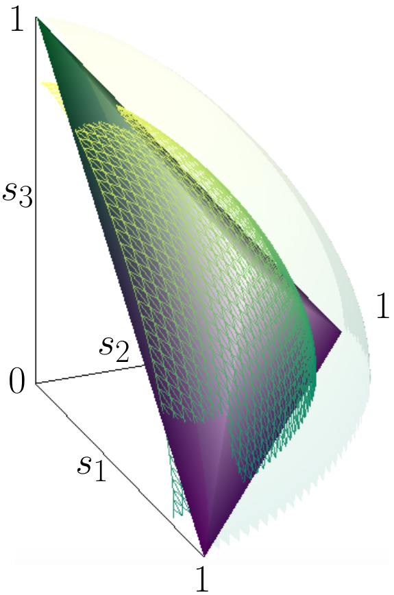
Figure 1: Separability, steerability with PVMs and POVMs of Bell-diagonal states. A general Bell-diagonal state is, up to local unitary transformations described by three parameters $(s_{1},s_{2},s_{3})$, which, without loosing generality, can be assumed to be positive. The states with all $s_{i}$ equal correspond to the Werner states. Using the original Barrett construction and the fact that separable states have an LHS model, one can see that the states in the volume characterized by the green-violet surface have an LHS model. The surface of states for which our model works ($R_{T}=6/5$) is shown as a yellow-green grid. The border of unsteerable states with projective measurements ($R_{T}=1$) is shown as a diaphanous surface. See the text for discussion.

V.2 Axially symmetric Bell-diagonal states

For the case of Bell-diagonal states with axial symmetry, $T=\operatorname{diag}(-s,-s,-t)$, the critical radius $R_{T}$ can be evaluated explicitly as  Nguyen et al. (2018)

$$R_{T}=\frac{1}{\left|t\right|}\frac{1}{1+x^{2}\frac{\operatorname{arctg}\sqrt{x^{2}-1}}{\sqrt{x^{2}-1}}},$$ (39)

where $x=s/t$ and $\sqrt{x^{2}-1}$ can take purely imaginary values when $\left|x\right|\leq 1$. With this, we find the axially symmetric Bell diagonal state is unsteerable with PVMs if and only if, $\left|t\right|^{-1}\geq 1+x^{2}/\sqrt{x^{2}-1}\operatorname{arctg}(\sqrt{x^{2}-1})$, and unsteerable with POVMs if $5/6\left|t\right|^{-1}\geq 1+x^{2}/\sqrt{x^{2}-1}\operatorname{arctg}(\sqrt{x^{2}-1})$.

V.3 General Bell-diagonal states

Let us finally discuss general Bell-diagonal states with $T=-\operatorname{diag}(s_{1},s_{2},s_{3})$. In the space of $(s_{1},s_{2},s_{3})$, the separable Bell diagonal states constitute an octahedron Horodecki and Horodecki (1996), which is symmetric under the three reflections $s_{i}\to-s_{i}$. Moreover $R_{T}$ depends only on the absolute values of $s_{i}$. We thus can concentrate on the steerability and separability of the Bell-diagonal states in the positive octant $s_{1}\geq 0$, $s_{2}\geq 0$, $s_{2}\geq 0$.

This situation is depicted in Fig. 1. In the positive octant, the border separating separable states from entangled state is a triangle with vertices $(1,0,0)$, $(0,1,0)$, $(0,0,1)$. Note that separable states are certainly unsteerable with POVMs. The original Barrett model for Werner states shows that the state corresponding to $(5/12,5/12,5/12)$ is also unsteerable with POVMs. Taking the convex hull of this point $(5/12,5/12,5/12)$ with those of the separable states, we obtain a polytope of states which are definitely unsteerable with POVMs. The faces of this polytopes are presented in Fig. 1 together with the surface $R_{T}=6/5$. The figure illustrates that our model demonstrates a significant new volume of Bell-diagonal states to be unsteerable with POVMs, in comparison to what has been known in the literature.

It should be noted, however, that our model does not work for all the states in the polytope mentioned above. In fact, the introduced model does not demonstrate the unsteerability of certain separable states, indicating that it is not optimal. Extrapolating to the Barrett’s original construction, one can expect that this well-known model is also not optimal. This is compatible with the conjecture that POVMs and PVMs are equivalent in quantum steering with the two-qubit Werner states, which is supported by some numerical evidence Werner (2014); Nguyen et al. (2018, 2019).

VI Conclusion

At first sight, Barrett’s construction of an LHS model for Werner states Barrett (2002) appears to be ad hoc. Our generalization illustrates a certain rational reasoning behind the construction. However, the very fact that Eq. (20) holds only came out though a rather complicated computation. The question whether this identity is a mathematical coincidence or there is a deeper mathematical reason underpinned it is an interesting question. We expect that the answer to this question can possibly lead to LHS models for a much more general class of bipartite states, shedding light on the role of POVMs in quantum steering and quantum nonlocality.