hIPPYlib: An Extensible Software Framework for Large-Scale Inverse Problems Governed by PDEs

Abstract.

We present an extensible software framework, hIPPYlib, for solution of large-scale deterministic and Bayesian inverse problems governed by partial differential equations (PDEs) with (possibly) infinite-dimensional parameter fields (which are high-dimensional after discretization). hIPPYlib overcomes the prohibitively expensive nature of Bayesian inversion for this class of problems by implementing state-of-the-art scalable algorithms for PDE-based inverse problems that exploit the structure of the underlying operators, notably the Hessian of the log-posterior. The key property of the algorithms implemented in hIPPYlib is that the solution of the inverse problem is computed at a cost, measured in linearized forward PDE solves, that is independent of the parameter dimension. The mean of the posterior is approximated by the MAP point, which is found by minimizing the negative log-posterior with an inexact matrix-free Newton-CG method. The posterior covariance is approximated by the inverse of the Hessian of the negative log posterior evaluated at the MAP point. The construction of the posterior covariance is made tractable by invoking a low-rank approximation of the Hessian of the log-likelihood. Scalable tools for sample generation are also discussed. hIPPYlib makes all of these advanced algorithms easily accessible to domain scientists and provides an environment that expedites the development of new algorithms.

1. Introduction

Recent years have seen tremendous growth in the volumes of observational and experimental data that are being collected, stored, processed, and analyzed. The central question that has emerged is: How do we extract knowledge and insight from all of this data? When the data correspond to observations of (natural or engineered) systems, and these systems can be represented by mathematical models, this knowledge-from-data problem is fundamentally a mathematical inverse problem. That is, given (possibly noisy) data and (a possibly uncertain) model, the goal becomes to infer parameters that characterize the model. Inverse problems abound in all areas of science, engineering, technology, and medicine. As just a few examples of model-based inverse problems, we may infer: the initial condition in a time-dependent partial differential equation (PDE) model, a coefficient field in a subsurface flow model, the ice sheet basal friction field from satellite observations of surface flow, the earth structure from reflected seismic waves, subsurface contaminant plume spread from crosswell electromagnetic measurements, internal structural defects from measurements of structural vibrations, ocean state from surface temperature observations, and so on.

Typically, inverse problems are ill-posed and suffer from non-unique solutions; simply put, the data—even when they are large-scale—do not provide sufficient information to fully determine the model parameters. This is the usual case with PDE models that have parameters representing fields such as boundary conditions, initial conditions, source terms, or heterogeneous coefficients. Non-uniqueness can stem from noise in the data or model, from sparsity of the data, from smoothing properties of the map from input model parameters to output observables or from its nonlinearity, or from intrinsic redundancy in the data. In such cases, uncertainty is a fundamental feature of the inverse problem. Therefore, not only do we wish to infer the parameters, but we must also quantify the uncertainty associated with this inference, reflecting the degree of “confidence” we have in the solution.

Methods that facilitate the solution of Bayesian inverse problems governed by complex PDE models require a diverse and advanced background in applied mathematics, scientific computing, and statistics to understand and implement, e.g., Bayesian inverse theory, computational statistics, inverse problems in function space, adjoint-based first- and second-order sensitivity analysis, and variational discretization methods. In addition, to be efficient these methods generally require first and second derivative (of output observables with respect to input parameters) information from the underlying forward PDE model, which can be cumbersome to derive. In this paper, we present hIPPYlib, an Inverse Problems Python library (hIPPYlib), an extensible software framework aimed at overcoming these challenges and providing capabilities for additional algorithmic developments for large-scale deterministic and Bayesian inversion.

hIPPYlib builds on FEniCS (a parallel finite element element library) (Logg et al., 2012) for the discretization of the PDEs, and on PETSc (Balay et al., 2014) for scalable and efficient linear algebra operations and solvers. Hence, it is easily applicable to medium to large-scale problems. One of the main features of this library is that it clearly displays and utilizes specific aspects from the model setup to the inverse solution, which can be useful not only for research purposes but also for learning and teaching. In the hIPPYlib examples, we show how to handle various PDE models and boundary conditions, and illustrate how to implement prior and log-likelihood terms for the Bayesian inference. hIPPYlib is implemented in a mixture of C++ and Python and has been released under the GNU General Public License version 2 (GPL). The source codes can be downloaded from https://hippylib.github.io. Below we summarize the main algorithmic and software contributions of hIPPYlib.

Algorithmic contributions

1. A single pass randomized eigensolver for generalized symmetric eigenproblems that is more accurate than the one proposed in (Saibaba et al., 2016).

2. A new scalable sampling algorithm for Gaussian random fields that exploits the structure of the given covariance operator. This extends the approach proposed in (Croci et al., 2018) to covariance operators defined as the inverse of second order differential operators as opposed to the identity operator.

3. A scalable algorithm to estimate the pointwise variance of Gaussian random fields using randomized eigensolvers. For the same computational cost this algorithm allows for more accurate estimates than the stochastic estimator proposed in (Bekas et al., 2007). Our method drastically reduces the variance of the estimator at a cost of introducing a small bias.

Software contributions

1. A modular approach to define complex inverse problems governed by (possibly nonlinear or time-dependent) PDEs. hIPPYlib automates the computation of higher order derivatives of the parameter-to-observable map for forward models and observation processes defined by the user through FEniCS.

2. Implementation of adjoints and Hessian actions needed to solve the deterministic inverse problem and to compute the maximum a posteriori (MAP) point of the Bayesian inverse problem. In addition, to test gradients and the Hessian action, hIPPYlib incorporates finite difference tests, which is an essential component of the verification process.

3. A robust implementation of the inexact Newton-conjugate gradient (Newton-CG) algorithm together with line search algorithms to guarantee global convergence of the optimizer.

4. Implementation of randomized algorithms to compute the low-rank factorization of the misfit part of the Hessian.

5. Scalable algorithms to construct and evaluate the Laplace approximation of the posterior.

6. Sampling capabilities to generate realizations of Gaussian random fields with a prescribed covariance operator.

7. An estimation of the pointwise variance of the prior distribution and Laplace approximation to the posterior.

Numerous toolkits and libraries for finite element computations based on variational forms are available, for instance COMSOL Multiphysics (COMSOL AB, 2009), deal.II (Bangerth et al., 2007), dune (Bastian et al., 2008), FEniCS (Logg et al., 2012; Langtangen and Logg, 2017), and Sundance, a package from Trilinos (Heroux et al., 2005). While these toolkits are usually tailored towards the solution of PDEs and systems of PDEs, they cannot be used straightforwardly for the solution of inverse problems with PDEs. However, several of them are sufficiently flexible to be extended for the solution of inverse problems governed by PDEs. Nevertheless, some knowledge of the structure underlying these packages is required since the optimality systems arising in inverse problems with PDEs often cannot be solved using generic PDE solvers, which do not exploit the optimization structure of the inverse problems. In (Farrell et al., 2013) the authors present dolfin-adjoint, a project that also builds on FEniCS and derives discrete adjoints from a forward model written in the Python interface to dolfin using a combination of symbolic and automatic differentiation. While dolfin-adjoint could be used to solve deterministic inverse problems, it lacks the framework for Bayesian inversion. In addition, we avoid using the adjoint capabilities of dolfin-adjoint since this does not allow the user to have full control over the construction of derivatives. In (Ruthotto et al., 2017) the authors present jInv, a flexible parallel software for parameter estimation with PDE forward models. The main limitations of this software are that it is restricted to deterministic inversion and that the user needs to provide the discretization for both the forward and adjoint problems. Finally, the Rapid Optimization Library, ROL (Kouri et al., 2018), is a flexible and robust optimization package in Trilinos for the solution of optimal design, optimal control and deterministic inverse problems in large-scale engineering applications. ROL implements state-of-the-art algorithms for unconstrained optimization, constrained optimization and optimization under uncertainty, and exposes an interface specific for optimization problems with PDE constraints. The main limitation is that the user has to interface with other software packages for the definition and implementation of the forward and adjoint problems. There also exist several general purpose libraries addressing uncertainty quantification (UQ) and Bayesian inverse problems. Among the most prominent we mention QUESO (McDougall et al., 2017; Prudencio and Schulz, 2012), DAKOTA (Eldred et al., 2002; Adams et al., 2009), PSUADE (Tong, 2017), UQTk (Debusschere et al., 2017). All of these libraries provide Bayesian inversion capabilities, but the underlying methods do not fully exploit the structure of the problem or make use of derivatives and as such are not intended for high-dimensional problems. Finally, MUQ (Parno et al., 2015) provides powerful Bayesian inversion models and algorithms, but expects forward models to come equipped with gradients/Hessians to permit large-scale solution.

In summary, to the best of our knowledge, there is no available software (open-source or otherwise) that provides all the discretization, optimization and statistical tools to enable scalable and efficient solution of deterministic and Bayesian inverse problems governed by complex PDE forward models. hIPPYlib is the first software framework that allows to tackle this specific class of inverse problems by facilitating the construction of forward PDE models equipped with adjoint/derivative information, providing state-of-the-art scalable optimization algorithms for the solution of the deterministic inverse problem and/or MAP point computation, and integrating tools for characterizing the posterior distribution.

The paper is structured as follows. Section 2 gives a brief overview of the deterministic and Bayesian formulation of inverse problems in an infinite-dimensional Hilbert space setting, and addresses the discretization of the underlying PDEs using the finite element method. Section 3 contains an overview of the design of the hIPPYlib software and of its components. Section 4 provides a detailed description of the algorithms implemented in hIPPYlib to solve the deterministic and linearized Bayesian inverse problem, namely the inexact Newton-CG algorithm, the single and double pass randomized algorithms for the solution of generalized hermitian eigenproblems, scalable sampling techniques for Gaussian random fields, and stochastic algorithms to approximate the pointwise variance of the prior and posterior distributions. Section 5 demonstrates hIPPYlib’s capabilities for deterministic and linearized Bayesian inversion by solving two representative inverse problems: inversion for the coefficient field in an elliptic PDE model and for the initial condition in an advection-diffusion PDE model. Last, Section 6 contains our concluding remarks.

2. Infinite-dimensional deterministic and Bayesian inverse problems in hIPPYlib

In what follows, we provide a brief account of the deterministic (Engl et al., 1996; Vogel, 2002) and Bayesian formulation (Tarantola, 2005; Kaipio and Somersalo, 2005) of inverse problems. Specifically, we adopt infinite-dimensional Bayesian inference framework (Stuart, 2010), and we refer to (Petra et al., 2014; Alexanderian et al., 2014, 2016; Bui-Thanh et al., 2013) for elaborations associated with discretization issues.

2.1. Deterministic inverse problems governed by PDEs

The inverse problem consists of using available observations $\boldsymbol{d}$ to infer the values of the unknown parameter field $m$ that characterize a physical process modeled by PDEs. Mathematically this inverse relationship is expressed as

(1) $$\boldsymbol{d}=\mathcal{F}(m)+\boldsymbol{\eta},$$

where the map $\mathcal{F}:\mathcal{M}\to\mathbb{R}^{q}$ is the so-called parameter-to-observable map. This mapping can be linear or nonlinear. In the applications targeted in hIPPYlib $\mathcal{M}\subseteq L^{2}(\mathcal{D})$, where $\mathcal{D}\subset\mathbb{R}^{d}$ is a bounded domain, and evaluations of $\mathcal{F}$ involve the solution of a PDE given $m$, followed by the application of an observation operator to extract the observations from the state. That is, introducing the state variable $u\in\mathcal{V}$ for a suitable Hilbert space $\mathcal{V}$ of functions defined on $\mathcal{D}$, the map $\mathcal{F}$ is defined as

(2) $$\mathcal{F}(m)=\mathcal{B}(u),\text{ s.t. }r(u,m)=0,$$

where $\mathcal{B}:\mathcal{V}\to\mathbb{R}^{q}$ is a (possibly nonlinear) observation operator, and $r:\mathcal{V}\times\mathcal{M}\to\mathcal{V}^{*}$—referred as the forward problem from now on—represents the PDE problem. The observations $\boldsymbol{d}$ contain noise due to measurement uncertainties and model errors (Tarantola, 2005). In (1), this is captured by the additive noise $\boldsymbol{\eta}$, which in hIPPYlib is modeled as $\boldsymbol{\eta}\sim\mathcal{N}\!\left({\boldsymbol{0}},{\boldsymbol{\Gamma}_{\!\mbox{\tiny noise}}}\right)$, i.e., a centered Gaussian at $\boldsymbol{0}$ with covariance $\boldsymbol{\Gamma}_{\!\mbox{\tiny noise}}$. A significant difficulty when solving infinite-dimensional inverse problems is that typically these are not well-posed (in the sense of Hadamard (Tikhonov and Arsenin, 1977)). To overcome the difficulties due to ill-posedness, we regularize the problem, i.e., we include additional assumptions on the solution, such as smoothness. The deterministic inverse problems in hIPPYlib are regularized via Tikhonov regularization, which penalizes oscillatory components of the parameter $m$, thus restricting the solution to smoothly varying fields (Engl et al., 1996; Vogel, 2002).

A deterministic inverse problem is therefore formulated as follows: given finite-dimensional noisy observations $\boldsymbol{d}\in\mathbb{R}^{q}$, one seeks to find the unknown parameter field $m$ that best reproduces the observations. Mathematically this translates into the following nonlinear least-squares minimization problem

(3) $$\min_{m\in\mathcal{M}}\!\mathcal{J}\left(m\right){:=}\frac{1}{2}\left\|\mathcal{F}(m)-\boldsymbol{d}\right\|^{2}_{\boldsymbol{\Gamma}_{\!\mbox{\tiny noise}}^{-1}}+\mathcal{R}(m),$$

where the first term in the cost functional, $\mathcal{J}\left(m\right)$, represents the misfit between the observations, $\boldsymbol{d}$, and that predicted by the parameter-to-observable map $\mathcal{F}(m)$, weighted by the inverse noise covariance $\boldsymbol{\Gamma}_{\!\mbox{\tiny noise}}^{-1}$. The regularization term, $\mathcal{R}(m)$, imposes regularity on the inversion field $m$, such as smoothness. As explained above, in the absence of such a term, the inverse problem is ill-posed, i.e., its solution is not unique and is highly sensitive to errors in the observations (Engl et al., 1996; Vogel, 2002).

As we will explain in Section 4.1, to efficiently solve the nonlinear least-squares problem (3) with parameter-to-observable-map $\mathcal{F}$ implicitly defined as in (2), first and second derivative information are needed. Using the Lagrangian formalism (Tröltzsch, 2010), abstract expressions for the gradient and Hessian action are obtained below, and we refer to Section 5 for concrete examples. To this aim, we introduce an auxiliary variable $p\in\mathcal{V}$, from here on referred as the adjoint, and write the Lagrangian functional

$$\mathcal{L}^{\mathcal{G}}(u,m,p):=\frac{1}{2}\|\mathcal{B}(u)-\boldsymbol{d}\|^{2}_{\boldsymbol{\Gamma}_{\!\mbox{\tiny noise}}^{-1}}+\mathcal{R}(m)+\,_{\mathcal{V}}\langle p,r(u,m)\rangle_{\mathcal{V}^{*}},$$

where ${}_{\mathcal{V}}\langle\cdot,\cdot\rangle_{\mathcal{V}^{*}}$ denotes the duality pair between $\mathcal{V}$ and its adjoint. The gradient for the cost functional (3) in an arbitrary direction $\tilde{m}\in\mathcal{M}$ evaluated at $m=m_{0}\in\mathcal{M}$ is the Gâteaux derivative of $\mathcal{L}$ with respect to $m$, and reads

(4) $$\left(\mathcal{G}(m_{0}),\tilde{m}\right)=\left(\mathcal{R}_{m}(m_{0}),\tilde{m}\right)+\,_{\mathcal{V}}\langle p_{0},r_{m}(u_{0},m_{0})[\tilde{m}]\rangle_{\mathcal{V}^{*}},\quad\forall\tilde{m}\in\mathcal{M},$$

where $\left(\mathcal{R}_{m}(m_{0}),\tilde{m}\right)\in\mathbb{R}$ denotes the Gâteaux derivative of $\mathcal{R}$ with respect to $m$ in the direction $\tilde{m}$ evaluated at $m=m_{0}$, and $r_{m}(u_{0},m_{0})[\tilde{m}]\in\mathcal{V}^{*}$ the Gâteaux derivative of $r$ with respect to $m$ in the direction $\tilde{m}$ evaluated at $u=u_{0},m=m_{0}$. Here $u_{0}$, $p_{0}$ are obtained by setting to zero the derivatives of $\mathcal{L}$ with respect to $p$ and $u$; specifically, $u_{0}$ solves the forward problem

(5) $$_{\mathcal{V}}\langle\tilde{p},r(u_{0},m_{0})\rangle_{\mathcal{V}^{*}}=0\quad\forall\tilde{p}\in\mathcal{V},$$

and $p_{0}$ solves the adjoint problem

(6) $$_{\mathcal{V}}\langle p_{0},r_{u}(u_{0},m_{0})[\tilde{u}]\rangle_{\mathcal{V}^{*}}+\langle\mathcal{B}_{u}(u_{0})[\tilde{u}],\mathcal{B}(u)-\boldsymbol{d}\rangle_{\mathbb{R}^{q}}=0,\quad\forall\tilde{u}\in\mathcal{V}.$$

In a similar way, to derive the expression for the Hessian action in an arbitrary direction $\hat{m}\in\mathcal{M}$ we introduce the second order Lagrangian functional

(7) $$\mathcal{L}^{\mathcal{H}}(u,m,p;\hat{u},\hat{m},\hat{p}) :=\left(\mathcal{G}(m),\hat{m}\right)$$

$$+_{\mathcal{V}}\langle\hat{p},r(u,m)\rangle_{\mathcal{V}^{*}}$$

$$+_{\mathcal{V}}\langle p,r_{u}(u,m)[\hat{u}]\rangle_{\mathcal{V}^{*}}+\langle\mathcal{B}_{u}(u)[\hat{u}],\mathcal{B}(u)-\boldsymbol{d}\rangle_{\mathbb{R}^{q}},$$

where the first term is the gradient expression, the second term stems from the forward problem, and the last two terms represent the adjoint problem. Then, the action of the Hessian in a direction $\hat{m}\in\mathcal{M}$ evaluated at $m=m_{0}$ is the variation of $\mathcal{L}^{\mathcal{H}}$ with respect to $m$ and reads

(8) $$\left(\tilde{m},\mathcal{H}(m_{0})\hat{m}\right) =\left(\tilde{m},\mathcal{R}_{mm}(m_{0})[\hat{m}]\right)+\left(p_{0},r_{mm}(u_{0},m_{0})[\tilde{m},\hat{m}]\right)$$

$$+_{\mathcal{V}}\langle\hat{p},r_{m}(u_{0},m_{0})[\tilde{m}]\rangle_{\mathcal{V}^{*}}+_{\mathcal{V}}\langle p_{0},r_{um}(u_{0},m_{0})[\hat{u},\tilde{m}]\rangle_{\mathcal{V}^{*}},\quad\forall m\in\mathcal{M}.$$

Here $u_{0}$, $p_{0}$ are the solution of the forward and adjoint problems (5) and (6), respectively. The incremental state $\hat{u}$ and incremental adjoint $\hat{p}$ solve the so-called incremental forward and incremental adjoint problems, which are obtained by setting to zero variations of $\mathcal{L}^{\mathcal{H}}$ with respect to $p$ and $u$, respectively. In Appendix A, we present a Newton-type algorithm to minimize (3) that uses the expression for the gradient (4) and Hessian action (8) derived here.

Finally, we note that the solution of a deterministic inverse problem based on regularization is a point estimate of $m$, which solves (1) in a least-squares sense. A systematic integration of the prior information on the model parameters and uncertainties associated with the observations can be achieved using a probabilistic point of view, where the prior information and noise model are represented by probability distributions. In the following section, we describe the probabilistic formulation of the inverse problem via a Bayesian framework, whose solution is a posterior probability distribution for $m$.

2.2. Bayesian inversion in infinite dimensions

In the Bayesian formulation in infinite dimensions, we state the inverse problem as a problem of statistical inference over the space of uncertain parameters, which are to be inferred from data and a physical model. In this setup, in contrast to the finite-dimensional case, there is no Lebesgue measure on $\mathcal{M}$, the infinite-dimensional Bayes formula is given by

(9) $$\frac{d\mu_{\mbox{\tiny post}}}{d\mu_{\mbox{\tiny prior}}}\propto\pi_{\mbox{\tiny like}}(\boldsymbol{d}|m).$$

Here, $d\mu_{\mbox{\tiny post}}/d\mu_{\mbox{\tiny prior}}$ denotes the Radon-Nikodym derivative (Williams, 1991) of the posterior measure $\mu_{\mbox{\tiny post}}$ with respect to $\mu_{\mbox{\tiny prior}}$, and $\pi_{\mbox{\tiny like}}(\boldsymbol{d}|m)$ denotes the data likelihood. Conditions under which the posterior measure is well defined and (9) holds are given in detail in (Stuart, 2010).

The noise model and the likelihood. In our hIPPYlib framework, we assume an additive noise model, $\boldsymbol{d}=\mathcal{F}(m)+\boldsymbol{\eta}$, where $\boldsymbol{\eta}\sim\mathcal{N}\!\left({\boldsymbol{0}},{\boldsymbol{\Gamma}_{\!\mbox{\tiny noise}}}\right)$ is a centered Gaussian on $\mathbb{R}^{q}$. This implies

(10) $$\pi_{\mbox{\tiny like}}(\boldsymbol{d}|m)\propto\exp\Big{\{}-\Phi(m)\Big{\}},$$

where $\Phi(m)=\frac{1}{2}\|\mathcal{F}(m)-\boldsymbol{d}\|^{2}_{\boldsymbol{\Gamma}_{\!\mbox{\tiny noise}}^{-1}}$ denotes the negative log-likelihood.

The prior. For many problems, it is reasonable to choose the prior to be Gaussian, i.e., $m\sim\mathcal{N}\!\left({m_{\text{pr}}},{\mathcal{C}_{\text{\tiny{prior}}}}\right)$. This implies

(11) $$d\mu_{\mbox{\tiny prior}}(m)\propto\exp\Big{\{}-\frac{1}{2}\|m-m_{\text{pr}}\|^{2}_{\mathcal{C}_{\text{\tiny{prior}}}^{-1}}\Big{\}}.$$

If the parameter represents a spatially correlated field defined on $\mathcal{D}\in\mathbb{R}^{d}$, the prior covariance operator $\mathcal{C}_{\text{\tiny{prior}}}$ usually imposes smoothness on the parameter. This is because rough components of the parameter field are typically cannot be inferred from the data, and must be determined by the prior to result in a well-posed Bayesian inverse problem.

In hIPPYlib we use elliptic PDE operators to construct the prior covariance, which allows us to capitalize on fast, optimal complexity solvers. More precisely, the prior covariance operator is the inverse of the $\nu$-th power ($\nu>\frac{d}{2}$) of a Laplacian-like operator, namely $\mathcal{C}_{\text{\tiny{prior}}}:=\mathcal{A}^{-\nu}=(-\gamma\,\boldsymbol{\Delta}+\delta I)^{-\nu}$, where $\gamma$, and $\delta>0$ control the correlation length $\rho$ and the pointwise variance $\sigma^{2}$ of the prior operator. Specifically, $\rho$—empirically defined as the distance $\rho$ for which the two-points correlation coefficient is 0.1—is proportional to $\sqrt{\gamma/\delta}$, and $\sigma^{2}$ is proportional to $\delta^{-\nu}\rho^{-d}$ (see e.g. (Lindgren et al., 2011) where exact expressions for $\rho$ and $\sigma^{2}$ as functions of $\gamma$ and $\delta$ are derived under the assumption of unbounded domain $\mathcal{D}$ and constant coefficients $\gamma$ and $\delta$). The coefficients $\gamma$ and $\delta$ can be constant (in which case the prior is stationary) or spatially varying. In addition, one can consider an anisotropic diffusion operator $\mathcal{A}=-\gamma\,\nabla\cdot(\boldsymbol{\Theta}\,\nabla)+\delta I$, with $\boldsymbol{\Theta}$ a symmetric positive definite (s.p.d.) tensor that models, for instance, stronger correlations in a specific direction. These choices of prior ensure that $\mathcal{C}_{\text{\tiny{prior}}}$ is a trace-class operator, guaranteeing bounded pointwise variance and a well-posed infinite-dimensional Bayesian inverse problem (Stuart, 2010; Bui-Thanh et al., 2013).

The posterior. Using the expression for the likelihood function (10) and prior distribution (11), the posterior distribution in (9) reads

(12) $$d\mu_{\mbox{\tiny post}}\propto\exp\Big{\{}-\frac{1}{2}\|\mathcal{F}(m)-\boldsymbol{d}\|^{2}_{\boldsymbol{\Gamma}_{\!\mbox{\tiny noise}}^{-1}}-\frac{1}{2}\|m-m_{\text{pr}}\|^{2}_{\mathcal{C}_{\text{\tiny{prior}}}^{-1}}\Big{\}}.$$

The maximum a posteriori (MAP) point $m_{\scriptscriptstyle\text{MAP}}$ is defined as the parameter field that maximizes the posterior distribution. It can be obtained by solving the following deterministic optimization problem

(13) $$m_{\scriptscriptstyle\text{MAP}}:=\operatorname*{argmin}_{m\in\mathcal{M}}(-\log d\mu_{\mbox{\tiny post}}(m))=\operatorname*{argmin}_{m\in\mathcal{M}}\frac{1}{2}\|\mathcal{F}(m)-\boldsymbol{d}\|^{2}_{\boldsymbol{\Gamma}_{\!\mbox{\tiny noise}}^{-1}}+\frac{1}{2}\|m-m_{\text{pr}}\|^{2}_{\mathcal{C}_{\text{\tiny{prior}}}^{-1}}.$$

We note that, the prior information plays the role of Tikhonov regularization in (3); in fact the deterministic optimization problem (3) is the same as (13) for the choice $\mathbb{R}(m)=\frac{1}{2}\|m-m_{\text{pr}}\|^{2}_{\mathcal{C}_{\text{\tiny{prior}}}^{-1}}$. The Hessian $\mathcal{H}(m_{\scriptscriptstyle\text{MAP}})$ of the negative log-posterior evaluated at $m_{\scriptscriptstyle\text{MAP}}$ plays a fundamental role in quantifying the uncertainty in the inferred parameter. In particular, this indicates which directions in the parameter space are most informed by the data (Bui-Thanh et al., 2013). We note that when $\mathcal{F}$ is linear, due to the particular choice of prior and noise model, the posterior measure is Gaussian, $\mathcal{N}\!\left({m_{\scriptscriptstyle\text{MAP}}},{\mathcal{C}_{\text{\tiny{post}}}}\right)$ with (Stuart, 2010, Section 6.4),

(14) $$\mathcal{C}_{\text{\tiny{post}}}=\mathcal{H}^{-1}=({\mathcal{F}}^{*}\boldsymbol{\Gamma}_{\!\mbox{\tiny noise}}^{-1}\mathcal{F}+\mathcal{C}_{\text{\tiny{prior}}}^{-1})^{-1},\qquad m_{\scriptscriptstyle\text{MAP}}=\mathcal{C}_{\text{\tiny{post}}}({\mathcal{F}}^{*}\boldsymbol{\Gamma}_{\!\mbox{\tiny noise}}^{-1}\boldsymbol{d}+\mathcal{C}_{\text{\tiny{prior}}}^{-1}m_{\text{pr}}),$$

where ${\mathcal{F}}^{*}:\mathbb{R}^{q}\to\mathcal{M}$ is the adjoint of $\mathcal{F}$.

In the general case of nonlinear parameter-to-observable map $\mathcal{F}$ the posterior distribution is not Gaussian. However, under certain assumptions on the noise covariance $\boldsymbol{\Gamma}_{\!\mbox{\tiny noise}}$, the number $q$ of observations, and the regularity of the parameter-to-observable map $\mathcal{F}$, the Laplace approximation (Stigler, S. M., 1986; Wong, 2001; Evans and Swartz, 2000; Press, 2003; Tierney and Kadane, 1986) can be invoked to estimate posterior expectations of functionals of the parameter $m$. Specifically, assuming that the negative log-likelihood $\Phi(m)$ is strictly convex in a neighborhood of $m_{\scriptscriptstyle\text{MAP}}$, the Laplace approximation to the posterior constructs a Gaussian distribution $\hat{\mu}_{\mbox{\tiny post}}$,

(15) $$\hat{\mu}_{\mbox{\tiny post}}\sim\mathcal{N}\!\left({m_{\scriptscriptstyle\text{MAP}}},{\mathcal{H}(m_{\scriptscriptstyle\text{MAP}})^{-1}}\right),$$

centered at $m_{\scriptscriptstyle\text{MAP}}$ and with covariance operator

(16) $$\mathcal{H}(m_{\scriptscriptstyle\text{MAP}})^{-1}=(\mathcal{H}_{\mbox{\tiny misfit}}(m_{\scriptscriptstyle\text{MAP}})+\mathcal{C}_{\text{\tiny{prior}}}^{-1})^{-1}.$$

Here $\mathcal{H}_{\mbox{\tiny misfit}}$ denotes the Hessian of the negative log-likelihood evaluated at $m_{\scriptscriptstyle\text{MAP}}$ (see Section 5 for examples of the derivation of the action of $\mathcal{H}_{\mbox{\tiny misfit}}$ using variational calculus and Lagrangian formalism).

The Laplace approximation above is an important tool in designing scalable and efficient methods for Bayesian inference and UQ implemented in hIPPYlib. It has been studied in the context of PDE-based inverse problems to draw approximate samples and compute approximate statistics (such as the pointwise variance) in (Bui-Thanh et al., 2013). Likewise, it has been exploited in (Petra et al., 2014) to efficiently explore the true posterior distribution by generating high quality proposals for Markov chain Monte Carlo algorithms, in (Cui et al., 2014b) to construct likelihood informed subspaces that allows for optimal dimension reduction in Bayesian inference problems, and in (Schillings, Claudia and Schwab, Christoph, 2016; Chen et al., 2017) to construct a dimension independent sparse grid to evaluate posterior expectations. It has also been invoked in (Isaac et al., 2015) for scalable approximation of the predictive posterior distribution of a scalar quantity of interest. Finally, its use was advocated in (Long et al., 2013, 2015b, 2015a; Alexanderian et al., 2016) to approximate the solution of Bayesian optimal experimental design problems.

2.3. Discretization of the Bayesian inverse problem

We present a brief discussion of the finite-dimensional approximations of the prior and the posterior distributions; a lengthier discussion can be found in (Bui-Thanh et al., 2013). We start with a finite-dimensional subspace $\mathcal{M}_{h}$ of $\mathcal{M}\subseteq L^{2}(\mathcal{D})$ originating from a finite element discretization with continuous Lagrange basis functions $\left\{\phi_{j}\right\}_{j=1}^{n}$ (Becker et al., 1981; Strang and Fix, 1988). The approximation of the inversion parameter function $m\in\mathcal{M}$ is then $m_{h}=\sum_{j=1}^{n}m_{j}\phi_{j}\in\mathcal{M}_{h}$, and, in what follows, $\boldsymbol{m}=\left(m_{1},\ldots,m_{n}\right)^{T}\in\mathbb{R}^{n}$ denotes the vector of the coefficients in the finite element expansion of $m_{h}$.

The finite-dimensional space $\mathcal{M}_{h}$ inherits the $L^{2}$-inner product. Thus, inner products between nodal coefficient vectors must be weighted by a mass matrix $\mathbf{{M}}\in\mathbb{R}^{n\times n}$ to approximate the infinite-dimensional $L^{2}$-inner product. This $\mathbf{{M}}$-weighted inner product is denoted by $\left\langle{\cdot\,},{\cdot}\right\rangle_{\!\scriptscriptstyle{\text{M}}}$, where $\left\langle{\boldsymbol{y}},{\boldsymbol{z}}\right\rangle_{\!\scriptscriptstyle{\text{M}}}=\boldsymbol{y}^{T}\mathbf{{M}}\boldsymbol{z}$ and $\mathbf{{M}}$ is the (symmetric positive definite) mass matrix

$$M_{ij}=\int_{\mathcal{D}}\phi_{i}(\boldsymbol{x})\phi_{j}(\boldsymbol{x})\,d\boldsymbol{x}~{},\quad i,j=1,\ldots,n.$$

To distinguish $\mathbb{R}^{n}$ equipped with the $\mathbf{{M}}$-weighted inner product with the usual Euclidean space $\mathbb{R}^{n}$, we denote it by $\mathbb{R}^{n}_{\mathbf{{M}}}$. For an operator $\mathbf{{B}}:\mathbb{R}^{n}_{\mathbf{{M}}}\rightarrow\mathbb{R}^{n}_{\mathbf{{M}}}$, we denote the matrix transpose by $\mathbf{{B}}^{T}$ with entries $(B^{T})_{ij}=B_{ji}$. In contrast, the $\mathbf{{M}}$-weighted inner product adjoint $\mathbf{{B}}^{*}$ satisfies, for $\boldsymbol{y},\boldsymbol{z}\in\mathbb{R}^{n}$,

$$\left\langle{\mathbf{{B}}\boldsymbol{y}},{\boldsymbol{z}}\right\rangle_{\!\scriptscriptstyle{\text{M}}}=\left\langle{\boldsymbol{y}},{\mathbf{{B}}^{*}\boldsymbol{z}}\right\rangle_{\!\scriptscriptstyle{\text{M}}},$$

which implies that $\mathbf{{B}}^{*}$ is given by

(17) $${\mathbf{{B}}}^{*} =\mathbf{{M}}^{-1}\mathbf{{B}}^{T}\mathbf{{M}}.$$

With these definitions, the matrix representation of the bilinear form involving the elliptic PDE operator $\mathcal{A}^{n}$ defined in Section 2.2 is given by $\mathbf{{R}}$ whose components are

(18) $$R_{ij}=\int_{\mathcal{D}}\phi_{i}(\boldsymbol{x})\mathcal{A}^{\nu}\phi_{j}(\boldsymbol{x})\,d\boldsymbol{x},\quad i,j\in\left\{1,\ldots,n\right\}.$$

Finally, restating Bayes’ theorem with Gaussian noise and prior in finite dimensions, we obtain:

(19) $$\pi_{\mbox{\tiny post}}(\boldsymbol{m})\propto\exp\Big{(}-\frac{1}{2}\|{\mathbf{{F}}}(\boldsymbol{m})-\boldsymbol{d}_{\text{obs}}\|^{2}_{\boldsymbol{\Gamma}_{\!\mbox{\tiny noise}}^{-1}}-\frac{1}{2}\|\boldsymbol{m}-{\boldsymbol{m}}_{\mbox{\tiny pr}}\|^{2}_{\boldsymbol{\Gamma}_{\!\mbox{\tiny prior}}^{-1}}\Big{)},$$

where ${\boldsymbol{m}}_{\mbox{\tiny pr}}$ is the mean of the prior distribution, $\boldsymbol{\Gamma}_{\!\mbox{\tiny prior}}:=\mathbf{{R}}^{-1}\mathbf{{M}}\in\mathbb{R}^{n\times n}$ is the covariance matrix for the prior that arises upon discretization of $\mathcal{C}_{\text{\tiny{prior}}}$, and $\boldsymbol{\Gamma}_{\!\mbox{\tiny noise}}\in\mathbb{R}^{q\times q}$ is the covariance matrix for the noise. The method of choice to explore the full posterior is Markov chain Monte Carlo (MCMC), which samples the posterior so that sample statistics can be computed. MCMC for large-scale inverse problems is still prohibitive for expensive forward problems and high-dimensional parameter spaces; here we make a quadratic approximation of the negative log of the posterior (19), which results—as discussed in Section 2.2 in the continuous setting—in the Laplace approximation of the posterior given by

(20) $$\pi_{\mbox{\tiny post}}(\boldsymbol{m})\propto\mathcal{N}(\boldsymbol{{m}_{\mbox{\tiny MAP}}},\boldsymbol{\Gamma}_{\!\mbox{\tiny post}})$$

The mean of this approximate posterior distribution, $\boldsymbol{{m}_{\mbox{\tiny MAP}}}$, is the parameter vector maximizing the posterior (19), and is known as the maximum a posteriori (MAP) point. It can be found by minimizing the negative log-posterior, which amounts to solving the following optimization problem:

(21) $$\boldsymbol{{m}_{\mbox{\tiny MAP}}}:=\operatorname*{argmin}_{\boldsymbol{m}}(-\log\pi_{\mbox{\tiny post}}(\boldsymbol{m}))=\operatorname*{argmin}_{\boldsymbol{m}}\frac{1}{2}\|{\mathbf{{F}}}(\boldsymbol{m})-\boldsymbol{d}_{\text{obs}}\|^{2}_{\boldsymbol{\Gamma}_{\!\mbox{\tiny noise}}^{-1}}+\frac{1}{2}\|\boldsymbol{m}-{\boldsymbol{m}}_{\mbox{\tiny pr}}\|^{2}_{\boldsymbol{\Gamma}_{\!\mbox{\tiny prior}}^{-1}},$$

which is the discrete counterpart of problem (13). Denoting with $\tilde{\mathbf{{H}}}(\boldsymbol{{m}_{\mbox{\tiny MAP}}})$ and $\tilde{\mathbf{{H}}}_{\mbox{\tiny misfit}}(\boldsymbol{{m}_{\mbox{\tiny MAP}}})$ the matrix representations of, respectively, the second derivative of negative log-posterior $\mathcal{H}$ and log-likelihood $\mathcal{H}_{\mbox{\tiny misfit}}$ (i.e., the data misfit component of the Hessian) in the $\mathbf{{M}}$-weighted inner product, and assuming that $\tilde{\mathbf{{H}}}_{\mbox{\tiny misfit}}(\boldsymbol{{m}_{\mbox{\tiny MAP}}})$ is positive definite, the covariance matrix $\boldsymbol{\Gamma}_{\!\mbox{\tiny post}}$ in the Laplace approximation is given by

(22) $$\boldsymbol{\Gamma}_{\!\mbox{\tiny post}}=\tilde{\mathbf{{H}}}^{-1}(\boldsymbol{{m}_{\mbox{\tiny MAP}}})=\left(\tilde{\mathbf{{H}}}_{\mbox{\tiny misfit}}(\boldsymbol{{m}_{\mbox{\tiny MAP}}})+\boldsymbol{\Gamma}_{\!\mbox{\tiny prior}}^{-1}\right)^{-1}.$$

For simplicity of the presentation, in the following we will let $\mathbf{{H}}=\mathbf{{M}}\tilde{\mathbf{{H}}}$ and $\mathbf{{H}}_{\mbox{\tiny misfit}}=\mathbf{{M}}\tilde{\mathbf{{H}}}_{\mbox{\tiny misfit}}$ be the matrix representation of the Hessian with respect to the standard Euclidean inner product. Using this notation, and recalling that $\boldsymbol{\Gamma}_{\!\mbox{\tiny prior}}=\mathbf{{R}}^{-1}\mathbf{{M}}$, we rewrite (22) as

(23) $$\boldsymbol{\Gamma}_{\!\mbox{\tiny post}}=\mathbf{{H}}^{-1}(\boldsymbol{{m}_{\mbox{\tiny MAP}}})\,\mathbf{{M}}=\left(\mathbf{{H}}_{\mbox{\tiny misfit}}(\boldsymbol{{m}_{\mbox{\tiny MAP}}})+\mathbf{{R}}\right)^{-1}\,\mathbf{{M}}.$$

Equation (21) and (23) define the mean and covariance matrix of the Laplace approximation to the posterior in the discrete setting. In Section 4, we present scalable (with respect to the parameter dimension) algorithms to compute the discrete MAP point $\boldsymbol{{m}_{\mbox{\tiny MAP}}}$ and to efficiently manipulate the covariance matrix $\boldsymbol{\Gamma}_{\!\mbox{\tiny post}}$.

3. Design and software components of hIPPYlib

hIPPYlib implements state-of-the-art scalable algorithms for PDE-based deterministic and Bayesian inverse problems. It builds on FEniCS (a parallel finite element library) (Logg et al., 2012; Langtangen and Logg, 2017) for discretization of PDEs and on PETSc (Balay et al., 2014) for scalable and efficient linear algebra operations and solvers. In hIPPYlib the user can express the forward PDE and the likelihood in variational form using the friendly, compact, near-mathematical notation of FEniCS, which will then automatically generate efficient code for the discretization. Linear and nonlinear, stationary and time-dependent PDEs are supported in hIPPYlib. For stationary problems, gradient and Hessian information can be automatically generated by hIPPYlib using FEniCS symbolic differentiation of the relevant variational forms. For time-dependent problems, instead, symbolic differentiation can only be used for the spatial terms, and the contribution to gradients and Hessians arising from the time dynamics needs to be provided by the user. Noise and prior covariance operators are modeled as inverses of elliptic differential operators allowing us to build on fast multigrid solvers for elliptic operators without explicitly constructing the dense covariance operator. The main components, classes, and functionalities of hIPPYlib are summarized in Fig.  1. These include:

1. The hIPPYlib model component describes the inverse problem, i.e., the data misfit functional (negative log-likelihood), the prior information, and the forward problem. More specifically, the user can select from among a library of data misfit functionals—such as pointwise observations or continuous observations in the domain or on the boundary—or implement new ones using the prescribed interface. hIPPYlib offers a library of priors the user can choose from and allows for user-provided priors as well. Finally, the user needs to provide the forward problem either in the form of a FEniCS variational form or (for more complicated or time dependent problem) as a user-defined object. When using FEniCS variational forms, hIPPYlib is able to derive expressions for the gradient and Hessian-apply automatically using FEniCS’ symbolic differentiation. This means that for stationary problems the user will only have to provide the variational form of the forward problem. For more complex problems (e.g., time-dependent problems), hIPPYlib allows the user to implement their own derivatives.

2. The hIPPYlib algorithms component contains the numerical methods needed for solving the deterministic and linearized Bayesian inverse problems, i.e., the globalized inexact Newton-CG algorithm, randomized generalized eigensolvers, scalable sampling of Gaussian fields, and trace/diagonal estimators for large-scale not-explicitly-available covariance matrices. These algorithms are described in detail in Section 4.

3. The hIPPYlib outputs component includes the parameter-to-observable map (and its linear approximation), gradient evaluation and Hessian action, and Laplace approximation of the posterior distribution (MAP point and low-rank based representation of the posterior covariance operator). The hIPPYlib outputs can be utilized as inputs to other UQ software, e.g., the MIT Uncertainty Quantification Library (MUQ), to perform a full characterization of the posterior distribution using advanced dimension-independent Markov chain Monte Carlo simulation, requiring derivative information.

We refer to (Villa et al., 2020) for a detailed description of the modules, classes and functions implemented in hIPPYlib.

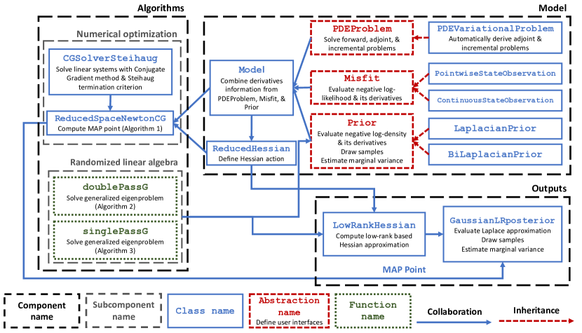
Figure 1. Design of the hIPPYlib framework. Red dotted connectors represent inheritance and blue solid connectors represent collaborations among the main components (black dashed boxes), classes (blue solid boxes and red dashed boxes), and functionalities (green dotted boxes) of hIPPYlib. The legend is shown on the bottom.

4. hIPPYlib algorithms

In this section we describe the main algorithms implemented in hIPPYlib for solution of deterministic and linearized Bayesian inverse problems. Specifically, we focus on computation of the MAP point and various operations on prior and posterior covariance matrices. In the linear case (and under the assumption of Gaussian noise and Gaussian prior) the posterior distribution is also Gaussian, and therefore is fully characterized once the MAP point and posterior covariance matrix are computed. In the nonlinear case, efficient exploration of the posterior distribution for large-scale PDE problems will require the use of a Markov chain Monte Carlo (MCMC) sampling method enchanted by Hessian information (see e.g. (Martin et al., 2012; Cui et al., 2014a; Cui et al., 2014c; Bui-Thanh and Girolami, 2014; Beskos et al., 2017)). In this case hIPPYlib provides the tools to generate proposals for MCMC.

4.1. Deterministic inversion and MAP point computation via inexact Newton-CG

hIPPYlib provides a robust implementation of the inexact Newton-conjugate gradient (Newton-CG) algorithm (e.g.,(Akçelik et al., 2006; Borzì and Schulz, 2012)) to solve the deterministic inverse problem and, in the Bayesian framework, to compute the maximum a posterior (MAP) point (see Algorithm 1). The gradient and Hessian actions—whose expressions are given in (4) and (8), respectively—are automatically computed via their variational form specification in FEniCS by constraining the state and adjoint variables to satisfy the forward and adjoint problem in (5) and (6) respectively. The Newton system is solved inexactly using early termination of CG iterations using Eisenstat–Walker (Eisenstat and Walker, 1996) (to prevent oversolving) and Steihaug (Steihaug, 1983) (to avoid negative curvature) criteria. Specifically, the choice of the tolerance $\eta_{i}$ in Algorithm 1 leads to superlinear convergence of Newton’s method, and represents a good compromise between the number of Newton iterations and the computational effort to compute the search direction. Globalization is achieved with an Armijo backtracking line search; we choose the Armijo constant $c_{\rm armijo}$ in the interval $[10^{-5},10^{-4}]$. For a wide class of nonlinear inverse problems, the number of outer Newton iterations and inner CG iterations is independent of the mesh size and hence parameter dimension (Heinkenschloss, 1993). This is a consequence of using Newton’s method, the compactness of the Hessian (of the data misfit term), and preconditioning with the inverse regularization operator. We note that the resulting preconditioned Hessian is a compact perturbation of the identity, for which Krylov subspace methods exhibit mesh-independent iterations (Campbell et al., 1996).

  $i\leftarrow 0$

  Given $\boldsymbol{m}_{0}$ solve the forward problem (5) to obtain $\boldsymbol{u}_{0}$

  Given $\boldsymbol{m}_{0}$ and $\boldsymbol{u}_{0}$ compute the cost functional $\mathcal{J}_{0}$ using (3)

  while $i<$ max_iter do

     Given $\boldsymbol{m}_{i}$ and $\boldsymbol{u}_{i}$ solve the adjoint problem (6) to obtain $\boldsymbol{p}_{i}$

     Given $\boldsymbol{m}_{i}$, $\boldsymbol{u}_{i}$ and $\boldsymbol{p}_{i}$ evaluate the gradient $\boldsymbol{g}_{i}$ using (4)

     if $\|\boldsymbol{g}_{i}\|\leq\tau$  then

        break

     end if

     Given $\boldsymbol{m}_{i}$, $\boldsymbol{u}_{i}$ and $\boldsymbol{p}_{i}$ define a linear operator $\mathbf{{H}}_{i}$ that implements the Hessian action (8)

     Using conjugate gradients, find a search direction $\widehat{\boldsymbol{m}}_{i}$ such that

$$\|\mathbf{{H}}_{i}\widehat{\boldsymbol{m}}_{i}+\boldsymbol{g}_{i}\|\leq\eta_{i}\|\boldsymbol{g}_{i}\|,\text{ with }\eta_{i}=\left(\frac{\|\boldsymbol{g}_{i}\|}{\|\boldsymbol{g}_{0}\|}\right)^{\frac{1}{2}}$$

     $j\leftarrow 0$, $\alpha^{(0)}\leftarrow 1$

     while $j<$ max_backtracking_iter do

        Set $\boldsymbol{m}^{(j)}=\boldsymbol{m}_{i}+\alpha^{(j)}\widehat{\boldsymbol{m}}_{i}$

        Given $\boldsymbol{m}^{(j)}$ solve the forward problem (5) to obtain $\boldsymbol{u}^{(j)}$

        Given $\boldsymbol{m}^{(j)}$ and $\boldsymbol{u}^{(j)}$ compute the cost $\mathcal{J}^{(j)}$ using (3)

        if  $\mathcal{J}^{(j)}<\mathcal{J}_{i}+\alpha^{(j)}c_{\rm armijo}\,\boldsymbol{g}_{i}^{T}\widehat{\boldsymbol{m}}_{i}$ then

           $\boldsymbol{m}_{i+1}\leftarrow\boldsymbol{m}^{(j)}$, $\mathcal{J}_{i+1}\leftarrow\mathcal{J}^{(j)}$

           break

        end if

        $\alpha^{(j+1)}\leftarrow\alpha^{(j)}/2,\quad j\leftarrow j+1$

     end while

     if $j=$ max_backtracking_iter then

        break

     end if

     $i\leftarrow i+1$

  end while

Algorithm 1 The inexact Newton-CG algorithm to find the MAP point

4.2. Low-rank approximation of the Hessian

The Hessian (of the negative log-posterior) plays a critical role in inverse problems. First, its spectral properties characterize the degree of ill-posedness. Second, the Hessian is the underlining operator for Newton-type optimization algorithms, which are highly desirable when solving inverse problems due to their dimension-independent convergence property. Third, the inverse of the Hessian locally characterizes the uncertainty in the solution of the inverse problem; under the Laplace approximation, it is precisely the posterior covariance matrix. Unfortunately, after discretization, the Hessian is formally a large, dense matrix; forming each column requires an incremental forward and adjoint solves (see Section 2.1). Thus, construction of the Hessian is prohibitive for large-scale problems since its dimension is equal to the dimension of the parameter. To make operations with the Hessian tractable, we exploit the fact that, in many cases, the eigenvalues collapse to zero rapidly, since the data contain limited information about the (infinite-dimensional) parameter field. Thus a low-rank approximation of the data misfit component of the Hessian, $\mathbf{{H}}_{\mbox{\tiny misfit}}$, can be constructed. This can be proven analytically for certain linear forward PDE problems (e.g. advection-diffusion (Flath et al., 2011), Poisson (Flath, 2013), Stokes (Worthen, 2012), acoustics (Bui-Thanh and Ghattas, 2012, 2013), electromagnetics (Bui-Thanh and Ghattas, 2013)), and demonstrated numerically for more complex PDE problems (e.g. seismic wave propagation (Bui-Thanh et al., 2013, 2012), mantle convection (Worthen et al., 2014), ice sheet flow (Isaac et al., 2015; Petra et al., 2014), poroelasticity (Hesse and Stadler, 2014), and turbulent flow (Chen et al., 2019)). The end result is that manipulations with the Hessian require a number of forward PDE solves that is independent of the parameter and data dimensions.

More specifically, to compute the low-rank factorization of the data misfit component of the Hessian we consider the following generalized symmetric eigenproblem:

(24) $$\mathbf{{H}}_{\mbox{\tiny misfit}}\boldsymbol{v}_{i}=\lambda_{i}\mathbf{{R}}\boldsymbol{v}_{i},\quad\lambda_{1}\geq\lambda_{2}\geq\ldots\geq\lambda_{n},$$

where $\mathbf{{R}}$ stems from the discretization (with respect to the Euclidean inner product) of the inverse of the prior covariance (i.e., the regularization operator). We then choose $r\ll n$ such that $\lambda_{r+i}$, $0<i\leq n-r$, is small relative to 1, and we define

$$\mathbf{{V}}_{r}=\begin{bmatrix}\boldsymbol{v}_{1},\boldsymbol{v}_{2},\ldots\boldsymbol{v}_{r}\end{bmatrix}\text{ and }\mathbf{{\Lambda}}_{r}={\rm diag}([\lambda_{1},\lambda_{2},\ldots,\lambda_{r}]),$$

where the matrix $\mathbf{{V}}_{r}$ has $\mathbf{{R}}$-orthonormal columns, that is $\mathbf{{V}}_{r}^{T}\mathbf{{R}}\mathbf{{V}}_{r}=\mathbf{{I}}_{r}$. As in (Isaac et al., 2015), by using the Sherman-Morrison-Woodbury formula, we write

(25) $$\mathbf{{H}}^{-1}=\left(\mathbf{{R}}+\mathbf{{H}}_{\mbox{\tiny misfit}}\right)^{-1}=\mathbf{{R}}^{-1}-\mathbf{{V}}_{r}\mathbf{{D}}_{r}\mathbf{{V}}_{r}^{T}+\mathcal{O}\left(\sum_{i=r+1}^{n}\frac{\lambda_{i}}{1+\lambda_{i}}\right),$$

where $\mathbf{{D}}_{r}=\operatorname{diag}(\lambda_{1}/(\lambda_{1}+1),\dots,\lambda_{r}/(\lambda_{r}+1))\in\mathbb{R}^{r\times r}$. As can be seen from the form of the remainder term above, to obtain an accurate low-rank approximation of $\mathbf{{H}}^{-1}$, we can neglect eigenvectors corresponding to eigenvalues that are small compared to 1. This result is used to efficiently apply the inverse and square-root inverse of the Hessian to a vector, as needed for computing the pointwise variance and when drawing samples from a Gaussian distribution with covariance $\mathbf{{H}}^{-1}$, as will be shown in Sections 4.3.2 and 4.4.2, respectively. Efficient algorithms implemented in hIPPYlib for solving eigenproblems using randomized linear algebra methods are described next.

4.2.1. Randomized algorithm for the generalized eigenvalue problem

Randomized algorithms for eigenvalue computations have proven to be extremely effective for matrices with rapidly decaying eigenvalues (Halko et al., 2011). For this class of matrices, in fact, randomized algorithms present several advantages compared to Krylov subspace methods. Krylov subspace methods require sophisticated algorithms to monitor restart, orthogonality, and loss of precision. On the contrary, randomized algorithm are easy to implement, can be made numerically robust, and expose more opportunities for parallelism since matrix-vector products can be done asynchronously across all vectors. The flexibility in reordering the computation makes randomized algorithms particularly well suited for modern parallel architectures with many cores per node and deep memory hierarchies.

In hIPPYlib we apply randomized algorithms to compute the low-rank factorization of the misfit part of the Hessian $\mathbf{{H}}_{\mbox{\tiny misfit}}$. With a change of notation, we write the generalized eigenvalue problem (24) as

(26) $$\mathbf{{A}}\boldsymbol{v}=\lambda\mathbf{{B}}\boldsymbol{v}$$

where $\mathbf{{A}}\in\mathbb{R}^{n\times n}$ is symmetric, $\mathbf{{B}}\in\mathbb{R}^{n\times n}$ is symmetric positive definite, and $\boldsymbol{v}\in\mathbb{R}^{n}$. Here we present an extension of the randomized eigensolvers in (Halko et al., 2011) to the solution of the generalized symmetric eigenproblem (26). Randomized algorithms for generalized symmetric eigenproblems were first introduced in (Saibaba et al., 2016), and are revisited here with some modifications.

The main idea behind randomized algorithms is to construct a matrix $\mathbf{{Q}}\in\mathbb{R}^{n\times(r+l)}$ with $\mathbf{{B}}$-orthonormal columns that approximates the range of $\mathbf{{B}}^{-1}\mathbf{{A}}$. Here, $r$ represents the number of eigenpairs we wish to compute, and $l$ is an oversampling factor. More specifically, we have

(27) $$\|(\mathbf{{I}}-\mathbf{{Q}}\mathbf{{Q}}^{T})\mathbf{{A}}\|_{\mathbf{{B}}}\leq\epsilon,$$

where $\epsilon$ is a random variable whose distribution depends on the generalized eigenvalues of (26) with index greater than $r+l$. To construct $\mathbf{{Q}}$, we let $\mathbf{{\Omega}}\in\mathbb{R}^{n\times(r+l)}$ be a Gaussian random matrix—whose entries are independent identically distributed (i.i.d.) standard Gaussian random variables—and we compute a $\mathbf{{B}}$-orthogonal basis for the range of $\mathbf{{Y}}=\mathbf{{B}}^{-1}\mathbf{{A}}\mathbf{{\Omega}}$ using the so called PreCholQR algorithm ((Lowery and Langou, 2014), see Algorithm 4). The main computational cost is the construction of $\mathbf{{Y}}$, which requires $(r+l)$ applications of the operator $\mathbf{{A}}$, and $(r+l)$ linear solves to apply $\mathbf{{B}}^{-1}$. In contrast, the computation of the matrix $\mathbf{{Q}}$ with $\mathbf{{B}}$-orthonormal columns using PreCholQR requires only an additional $(r+l)$ applications of $\mathbf{{B}}$ and $\mathcal{O}(n(r+l)^{2})$ dense linear algebra operations for the QR factorization. Using (27) it can be shown (see (Halko et al., 2011)) that $\mathbf{{A}}\approx(\mathbf{{B}}\mathbf{{Q}})(\mathbf{{Q}}^{T}\mathbf{{A}}\mathbf{{Q}})(\mathbf{{B}}\mathbf{{Q}})^{T}=(\mathbf{{B}}\mathbf{{Q}})\mathbf{{T}}(\mathbf{{B}}\mathbf{{Q}})^{T},$ where we have defined $\mathbf{{T}}:=\mathbf{{Q}}^{T}\mathbf{{A}}\mathbf{{Q}}$. Then we compute the eigendecomposion $\mathbf{{T}}=\mathbf{{S}}\mathbf{{\Lambda}}\mathbf{{S}}^{T}$ ($\mathbf{{S}}^{T}\mathbf{{S}}=\mathbf{{I}}_{r+l}$), and we approximate the $r$ dominant eigenpairs $(\mathbf{{\Lambda}}_{r},\mathbf{{V}}_{r})$ of (26) by:

(28) $$\mathbf{{\Lambda}}_{r}=\mathbf{{\Lambda}}(1:r,1:r),\quad\mathbf{{V}}_{r}=\mathbf{{Q}}\mathbf{{S}}(:,1:r).$$

Algorithms 2 and 3 summarize the implementation of the double pass and single pass randomized algorithms (Halko et al., 2011). The main difference between these two algorithms is how the small matrix $\mathbf{{T}}$ is computed. In the double pass algorithm, $\mathbf{{T}}$ is computed directly by performing a second round of multiplication $\mathbf{{A}}\mathbf{{Q}}$ with the operator $\mathbf{{A}}$. In the single pass algorithm, $\mathbf{{T}}$ is approximated from the information contained in $\mathbf{{\Omega}}$ and $\mathbf{{Y}}$. In particular, generalizing the single pass algorithm in (Halko et al., 2011) to (26), we approximate $\mathbf{{T}}$ as the least-squares solution of

(29) $$\mathbf{{T}}=\operatorname*{argmin}_{\mathbf{{X}}\in\mathbb{R}^{(r+l)\times(r+l)},s.s.p.d}\|\mathbf{{X}}(\mathbf{{Q}}^{T}\mathbf{{B}}\mathbf{{\Omega}})-\mathbf{{Q}}^{T}\mathbf{{B}}\mathbf{{Y}}\|^{2}_{2}.$$

For this reason, the single pass algorithm has a lower computational cost compared to the double pass algorithm; however the resulting approximation is less accurate. We remark that Algorithm 3 is more accurate than the single pass algorithm presented in (Saibaba et al., 2016). The key difference between the two algorithms is in the definition of $\mathbf{{T}}$. In (Saibaba et al., 2016), the authors define $\mathbf{{T}}=(\mathbf{{Q}}^{T}\mathbf{{B}}\mathbf{{\Omega}})^{-1}(\mathbf{{Q}}^{T}\mathbf{{B}}\mathbf{{Y}})(\mathbf{{Q}}^{T}\mathbf{{B}}\mathbf{{\Omega}})^{-1}$, while in Algorithm 3 we define $\mathbf{{T}}$ as the least-squares solution of (29). Fig.  2 numerically illustrates the higher accuracy of the proposed approach when computing the first 30 eigenvalues of the data misfit Hessian discussed in Section 5.1.

  Let $r$ be the number of eigenpairs to compute and $l$ an oversampling factor

  Let $\mathbf{{\Omega}}\in\mathbb{R}^{n\times(r+l)}$ be a Gaussian random matrix

  $\bar{\mathbf{{Y}}}\leftarrow\mathbf{{A}}\mathbf{{\Omega}}$, $\mathbf{{Y}}=\mathbf{{B}}^{-1}\bar{\mathbf{{Y}}}$

  Use PreCholQR to factorize $\mathbf{{Y}}=\mathbf{{Q}}\mathbf{{R}}$ such that $\mathbf{{Q}}^{T}\mathbf{{B}}\mathbf{{Q}}=\mathbf{{I}}_{r+l}$

  $\mathbf{{T}}\leftarrow\mathbf{{Q}}^{T}\mathbf{{A}}\mathbf{{Q}}$

  Compute the eigenvalue decomposition $\mathbf{{T}}=\mathbf{{S}}\mathbf{{\Lambda}}\mathbf{{S}}^{T}$

  Keep the $r$ largest eigenmodes and let $\mathbf{{S}}_{r}\leftarrow\mathbf{{S}}(:,1:r)$, $\mathbf{{\Lambda}}_{r}\leftarrow\mathbf{{\Lambda}}(1:r,1:r)$

  Return: $\mathbf{{V}}_{r}\leftarrow\mathbf{{Q}}\mathbf{{S}}_{r}$, and $\mathbf{{\Lambda}}_{r}$

Algorithm 2 The double pass randomized algorithm for the solution of the generalized symmetric eigenproblem.

  Let $r$ be the number of eigenpairs to compute and $l$ an oversampling factor

  Let $\mathbf{{\Omega}}\in\mathbb{R}^{n\times(r+l)}$ be a Gaussian random matrix

  $\bar{\mathbf{{Y}}}\leftarrow\mathbf{{A}}\mathbf{{\Omega}}$, $\mathbf{{Y}}=\mathbf{{B}}^{-1}\bar{\mathbf{{Y}}}$

  Use PreCholQR to factorize $\mathbf{{Y}}=\mathbf{{Q}}\mathbf{{R}}$ such that $\mathbf{{Q}}^{T}\mathbf{{B}}\mathbf{{Q}}=\mathbf{{I}}_{r+l}$ and $\bar{\mathbf{{Q}}}$ such that $\bar{\mathbf{{Q}}}^{T}\mathbf{{B}}^{-1}\bar{\mathbf{{Q}}}=\mathbf{{I}}_{r+l}$

  Find $\mathbf{{T}}$ s.s.p.d such that $\|\mathbf{{T}}(\bar{\mathbf{{Q}}}^{T}\mathbf{{\Omega}})-\bar{\mathbf{{Q}}}^{T}\mathbf{{Y}}\|^{2}_{2}\rightarrow\min$

  Compute the eigenvalue decomposition $\mathbf{{T}}=\mathbf{{S}}\mathbf{{\Lambda}}\mathbf{{S}}^{T}$

  Keep the $r$ largest eigenmodes and let $\mathbf{{S}}_{r}\leftarrow\mathbf{{S}}(:,1:r)$, $\mathbf{{\Lambda}}_{r}\leftarrow\mathbf{{\Lambda}}(1:r,1:r)$

  Return: $\mathbf{{V}}_{r}\leftarrow\mathbf{{Q}}\mathbf{{S}}_{r}$, and $\mathbf{{\Lambda}}_{r}$

Algorithm 3 The single pass randomized algorithm for the solution of the generalized symmetric eigenproblem.

  Require: $\mathbf{{Y}}\in\mathbb{R}^{n\times(r+l)}$, and $\mathbf{{B}}\in\mathbb{R}^{n\times n}$

  $[\mathbf{{Z}},\mathbf{{R}}_{\mathbf{{Y}}}]\leftarrow{\rm qr}(\mathbf{{Y}})$

  $\bar{\mathbf{{Z}}}\leftarrow\mathbf{{B}}\mathbf{{Z}}$

  $\mathbf{{R}}_{\mathbf{{Z}}}={\rm chol}(\mathbf{{Z}}^{T}\bar{\mathbf{{Z}}})$

  Return: $\mathbf{{Q}}=\mathbf{{Z}}\mathbf{{R}}_{\mathbf{{Z}}}^{-1}$, $\bar{\mathbf{{Q}}}=\bar{\mathbf{{Z}}}\mathbf{{R}}_{\mathbf{{Z}}}^{-1}$, and $\mathbf{{R}}=\mathbf{{R}}_{\mathbf{{Z}}}\mathbf{{R}}_{\mathbf{{Y}}}$

Algorithm 4 PreCholQR

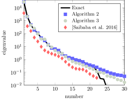
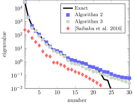
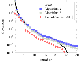
Figure 2. Log-linear plot of first 30 out of 4225 generalized eigenvalues of the data misfit Hessian in Section 5.1. A deterministic eigensolver (Exact), Algorithm 2, Algorithm 3, and the single pass algorithm in (Saibaba et al., 2016) are compared for different choices of the oversampling parameter $l$ (left $l=5$, center $l=10$, right $l=20$). Note that Algorithm 3 is more accurate for the single pass algorithm in (Saibaba et al., 2016) for all choices of $l$.

4.3. Sampling from large-scale Gaussian random fields

Sampling techniques play a fundamental role in exploring the posterior distribution and in quantifying the uncertainty in the inferred parameter; for example, Markov chain Monte Carlo methods often use the prior distribution (assumed Gaussian in our settings) or some Gaussian approximation to the posterior to generate proposals for the Metropolis-Hastings algorithm. In this section, we describe the sampling capabilities implemented in hIPPYlib to generate realizations of Gaussian random fields with a prescribed covariance operator $\mathcal{C}$. Then we describe how the low-rank factorization of the data misfit part of the Hessian in Section 4.2 can be exploited to generate samples from the Laplace approximation of the posterior distribution in (15). In what follows, we will denote the expected value (mean) of a random vector $\boldsymbol{x}$ with the symbol $\mathsf{E}\left[\boldsymbol{x}\right]$, and its covariance with the symbol ${\rm cov}(\boldsymbol{x}):=\mathsf{E}\big{[}\left(\boldsymbol{x}-\mathsf{E}[\boldsymbol{x}]\right)\left(\boldsymbol{x}-\mathsf{E}[\boldsymbol{x}]\right)^{T}\big{]}$. We will also denote with $\mathbf{{\Gamma}}$ the matrix representation of the covariance operator $\mathcal{C}$ with respect to the standard Euclidean inner product.

To sample from a small-scale multivariate Gaussian distribution, it is common to resort to a Cholesky factorization of the covariance matrix $\mathbf{{\Gamma}}=\mathbf{{C}}\mathbf{{C}}^{T}$. In fact, if $\boldsymbol{\eta}$ is a vector of independent identically distributed Gaussian variables $\eta_{i}$ with zero mean ($\mathsf{E}\left[\boldsymbol{\eta}\right]=\boldsymbol{0}$ ) and unit variance (${\rm cov}(\boldsymbol{\eta})=\mathbf{{I}}$), then $\boldsymbol{x}=\mathbf{{C}}\boldsymbol{\eta}$ is such that

$${\rm cov}(\boldsymbol{x})=\mathsf{E}\left[\boldsymbol{x}\boldsymbol{x}^{T}\right]=\mathsf{E}\left[\mathbf{{C}}\boldsymbol{\eta}\boldsymbol{\eta}^{T}\mathbf{{C}}^{T}\right]=\mathbf{{C}}\mathsf{E}\left[\boldsymbol{\eta}\boldsymbol{\eta}^{T}\right]\mathbf{{C}}^{T}=\mathbf{{C}}\mathbf{{C}}^{T}=\mathbf{{\Gamma}}.$$

Since an affine transformation of a Gaussian vector is still Gaussian, we have that $\boldsymbol{x}\sim\mathcal{N}(\boldsymbol{0},\mathbf{{\Gamma}})$.

This approach is not feasible for large-scale problems since it requires computing the Cholesky factorization of the covariance matrix. However, note that a decomposition of the form $\mathbf{{\Gamma}}=\mathbf{{C}}\mathbf{{C}}^{T}$ can be obtained using a matrix $C$ other than the Cholesky factor. In particular, the matrix $\mathbf{{C}}$ need not be a triangular, or even square, matrix. In Appendix C, we exploit this observation and show a scalable sampling technique based on a rectangular decomposition of $\mathbf{{R}}=\mathbf{{\Gamma}}^{-1}$, for the case when $\mathbf{{R}}$ is a finite element discretization of a differential operator. We note that a similar approach was, independently, investigated in (Croci et al., 2018) to sample realizations of white noise by exploiting a rectangular decomposition of the finite element mass matrix. Our approach is more general as it allows for decomposing matrices stemming from finite element discretization of operators other than identity.

4.3.1. Sampling from the prior

Sampling from a Gaussian distribution with a prescribed covariance matrix $\mathbf{{\Gamma}}$ is a difficult task for large-scale problems. Different approaches have been investigated, but how to make these algorithms scalable is still an active area of research. In (Parker and Fox, 2012), the authors introduce a conjugate gradient sampler that is a simple extension of the conjugate gradient method for solving linear systems. However, loss of orthogonality in finite arithmetic and the need of a factorized preconditioner limit the efficiency of this sampler for large-scale applications. In (Chow and Saad, 2014), the authors consider a preconditioned Krylov subspace method to approximate the action of $\mathbf{{\Gamma}}^{\frac{1}{2}}$ on a generic vector $z$. In (Chen et al., 2011), the authors discuss a method to compute $f(\mathbf{{\Gamma}})\boldsymbol{b}$ via least-squares polynomial approximations for a generic matrix function $f(x)=\sqrt{x}$. To this aim the authors approximate the function by a spline of a desired accuracy on the spectrum of $\mathbf{{\Gamma}}$ and introduce a weighted inner product to simplify the computation.

hIPPYlib implements a new sampling algorithm that strongly relies on the structure of the covariance matrix and on the assembly procedure of finite element matrices. In particular, we restrict ourselves to the class of priors described in Section 2.2. For this class of priors, the inverse of the covariance matrix admits a sparse representation as a finite element matrix $\mathbf{{R}}$ stemming from the finite element discretization of a coercive symmetric differential operator. To draw a sample $\boldsymbol{x}$ from the distribution $\mathcal{N}\left(\boldsymbol{0},\mathbf{{R}}^{-1}\right)$, we solve the linear system

(30) $$\mathbf{{R}}\boldsymbol{x}=\mathbf{{C}}\boldsymbol{\eta},\text{ where }\boldsymbol{\eta}\sim\mathcal{N}\left(\boldsymbol{0},\mathbf{{I}}_{q}\right),$$

where $\mathbf{{C}}\in\mathbb{R}^{n\times q}$ ($q\geq n$) is the rectangular factor of $\mathbf{{R}}$ described in Appendix C. In particular, we have

$$\mathsf{E}[\boldsymbol{x}\boldsymbol{x}^{T}]=\mathbf{{R}}^{-1}\mathbf{{C}}\mathsf{E}[\boldsymbol{\eta}\boldsymbol{\eta}^{T}]\mathbf{{C}}^{T}\mathbf{{R}}^{-1}=\mathbf{{R}}^{-1}\,\mathbf{{R}}\,\mathbf{{R}}^{-1}=\mathbf{{R}}^{-1},$$

where we exploited the fact that $\mathsf{E}[\boldsymbol{\eta}\boldsymbol{\eta}^{T}]=\mathbf{{I}}_{q}$ and $\mathbf{{C}}\mathbf{{C}}^{T}=\mathbf{{R}}$. This method is particularly efficient at large-scale since: i) the matrix $\mathbf{{C}}$ is sparse and can be computed efficiently by exploiting the finite element assembly routine; ii) the dominant cost is the solution of a linear system with coefficient matrix $\mathbf{{R}}$, for which efficient and scalable methods are available (e.g. conjugate gradients with algebraic multigrid preconditioner); and iii) the stochastic dimension of $\boldsymbol{\eta}$ also scales linearly with the size of the problem.

4.3.2. Sampling from the Laplace approximation of the posterior

To sample from the Laplace approximation of the posterior we assume that the posterior covariance operator can be expressed as a low-rank update of the prior covariance, i.e., in the form of equation (25). This assumption is often verified for many inverse problems as we discussed in Section 4.2. Then given a sample from the prior distribution $\boldsymbol{x}\sim\mathcal{N}\left(\boldsymbol{0},\mathbf{{R}}^{-1}\right)$, a sample from the Laplace approximation of the posterior $\mathcal{N}\left(\mathbf{{0}},(\mathbf{{H}}_{\mbox{\tiny misfit}}+\mathbf{{R}})^{-1}\right)$ can be computed as

(31) $$\boldsymbol{y}=\left(\mathbf{{I}}_{n}-\mathbf{{V}}_{r}\mathbf{{S}}_{r}\mathbf{{V}}_{r}^{T}\mathbf{{R}}\right)\boldsymbol{x},$$

where $\mathbf{{S}}_{r}=\mathbf{{I}}_{r}-(\mathbf{{\Lambda}}_{r}+\mathbf{{I}}_{r})^{-\frac{1}{2}}=\operatorname{diag}(1-1/\sqrt{\lambda_{1}+1},\dots,1-1/\sqrt{\lambda_{r}+1})\in\mathbb{R}^{r\times r}$. This can be verified by the following calculation,

$${\rm cov}(\boldsymbol{y})=\mathsf{E}\left[\boldsymbol{y}\boldsymbol{y}^{T}\right] =\mathsf{E}\left[\left(\mathbf{{I}}_{n}-\mathbf{{V}}_{r}\mathbf{{S}}_{r}\mathbf{{V}}_{r}^{T}\mathbf{{R}}\right)\boldsymbol{x}\boldsymbol{x}^{T}\left(\mathbf{{I}}_{n}-\mathbf{{V}}_{r}\mathbf{{S}}_{r}\mathbf{{V}}_{r}^{T}\mathbf{{R}}\right)^{T}\right]$$

$$=\left(\mathbf{{I}}_{n}-\mathbf{{V}}_{r}\mathbf{{S}}_{r}\mathbf{{V}}_{r}^{T}\mathbf{{R}}\right)\mathsf{E}\left[\boldsymbol{x}\boldsymbol{x}^{T}\right]\left(\mathbf{{I}}_{n}-\mathbf{{V}}_{r}\mathbf{{S}}_{r}\mathbf{{V}}_{r}^{T}\mathbf{{R}}\right)^{T}$$

$$=\left(\mathbf{{I}}_{n}-\mathbf{{V}}_{r}\mathbf{{S}}_{r}\mathbf{{V}}_{r}^{T}\mathbf{{R}}\right)\mathbf{{R}}^{-1}\left(\mathbf{{I}}_{n}-\mathbf{{V}}_{r}\mathbf{{S}}_{r}\mathbf{{V}}_{r}^{T}\mathbf{{R}}\right)^{T}$$

$$=\mathbf{{R}}^{-1}-\mathbf{{V}}_{r}(2\mathbf{{S}}_{r}-\mathbf{{S}}_{r}^{2})\mathbf{{V}}_{r}^{T}$$

$$=\mathbf{{R}}^{-1}-\mathbf{{V}}_{r}\mathbf{{D}}_{r}\mathbf{{V}}_{r}^{T}\approx\mathbf{{H}}^{-1},$$

where we have used the definition of $\mathbf{{D}}_{r}$, the $\mathbf{{R}}$-orthogonality of the eigenvectors matrix $\mathbf{{V}}_{r}$ (i.e., $\mathbf{{V}}_{r}^{T}\mathbf{{R}}\mathbf{{V}}_{r}=\mathbf{{I}}_{r}$), and the fact that

$$2\left(1-\frac{1}{\sqrt{1+\lambda_{i}}}\right)\!-\!\left(1-\frac{1}{\sqrt{1+\lambda_{i}}}\right)^{2}\!=\!1-\left[\left(1-\frac{1}{\sqrt{1+\lambda_{i}}}\right)\!-\!1\right]^{2}=\frac{\lambda_{i}}{1+\lambda_{i}}.$$

4.4. Pointwise variance of Gaussian random fields

Consider a Gaussian random field $m\sim\mathcal{N}\left(0,\mathcal{C}\right)$ and its discrete counterpart $\boldsymbol{m}\sim\mathcal{N}\left(\boldsymbol{0},\mathbf{{Q}}^{-1}\right)$, where $\mathbf{{Q}}$ is the precision matrix. Here $\mathcal{C}=\mathcal{C}_{\rm pr}$ and $\mathbf{{Q}}=\mathbf{{R}}$ if we are interested in the prior distribution; $\mathcal{C}=\mathcal{C}_{\rm post}$ and $\mathbf{{Q}}=\mathbf{{H}}$ for the posterior distribution. Then we define the pointwise variance of $m$ as the field $\sigma^{2}(x)$ such that

$$\sigma^{2}(x)={\rm Var}[m(x)],\quad\forall x\in\mathcal{D}.$$

In this section, we present an efficient numerical method to compute a finite element approximation $\sigma_{h}^{2}$ of $\sigma^{2}(x)$. As shown in (Bui-Thanh et al., 2013), the diagonal of $Q^{-1}$ (i.e., ${\rm diag}(\mathbf{{Q}}^{-1})$) is the vector corresponding to the coefficients of the expansion of $\sigma_{h}^{2}$ in the finite element basis. A naïve approach would require solution of $n$ linear systems with $\mathbf{{Q}}$. This is not feasible for large-scale problems: even for the case when an optimal (i.e., $\mathcal{O}(n)$) solver for $\mathbf{{Q}}$ is available, the complexity is at least $\mathcal{O}(n^{2})$ operations. In what follows we discuss stochastic estimators and probing methods to efficiently estimate the pointwise variance of the prior distribution and we explore how the low-rank representation of the data misfit component of the Hessian can be efficiently exploited to compute the pointwise variance of the Laplace approximation of posterior distribution.

4.4.1. Pointwise variance of the prior

Estimating the pointwise variance of the prior reduces to the well studied problem of estimating the diagonal of the inverse of a matrix $\mathbf{{R}}$. Recall that in our case, $\mathbf{{R}}$ arises from finite element discretization of an elliptic differential operator. Two commonly used methods to solve this task are the stochastic estimator in (Bekas et al., 2007) and the probing method in (Tang and Saad, 2012). Specifically, the unbiased stochastic estimator for the diagonal of the inverse of $\mathbf{{R}}$ in (Bekas et al., 2007) reads

(32) $${\rm diag}(\mathbf{{R}}^{-1})\approx\left[\sum_{j=1}^{s}\boldsymbol{z}_{j}\odot\boldsymbol{w}_{j}\right]\oslash\left[\sum_{j=1}^{s}\boldsymbol{z}_{j}\odot\boldsymbol{z}_{j}\right],$$

where $\boldsymbol{w}_{j}$ solves $\mathbf{{R}}\boldsymbol{w}_{j}=\boldsymbol{z}_{j}$ and $\boldsymbol{z}_{j}$ are random i.i.d. vectors. Here $\odot$ and $\oslash$ represent the element-wise multiplication and division operators of vectors, respectively. The convergence of the method is independent of the size of the problem, but convergence is in general slow. The probing method in (Tang and Saad, 2012), on the other hand, leads to faster convergence in the common situation in which $\mathbf{{R}}^{-1}$ exhibits a decay property, i.e., the entries far away from the diagonal are small. Probing vectors are determined by applying some coloring algorithm to the graph $\mathcal{G}$ whose adjacency matrix is the sparsity pattern of some power $k$ of $\mathbf{{R}}$. More specifically, there are as many probing vectors as the number of colors in the graph $\mathcal{G}$ and the probing vector associated to color $i$ is the binary vector whose non-zero entries correspond to the nodes of $\mathcal{G}$ colored with color $i$. The higher the power $k$, the more accurate will be the estimation, but also the more expensive due to the increased number of colors (and, therefore, of probing vectors to solve for). The main shortcoming of this approach is that it is not mesh independent, i.e., as we refine the mesh we need to increase the power $k$ and therefore the number of probing vectors.

To overcome these difficulties, hIPPYlib implements, in addition to the methods mentioned above, a novel approach based on a randomized eigendecomposition of $\mathbf{{R}}^{-1}$, taking advantage of the fact that $\mathbf{{R}}$ is the discretization of an elliptic differential operator. Specifically, we write

(33) $${\rm diag}(\mathbf{{R}}^{-1})\approx\left[\sum_{i=1}^{\overline{r}}\mu_{i}\overline{{\boldsymbol{v}}}_{i}\odot\overline{{\boldsymbol{v}}}_{i}\right],$$

where $\{(\mu_{i},\overline{\boldsymbol{v}}_{i})\}_{1}^{\overline{r}}$ denote the approximation of the $\overline{r}$ dominant eigenpairs of the matrix $\mathbf{{R}}^{-1}$ obtained by using the double pass randomized eigensolver (Algorithm 2) with $l=0$, $\mathbf{{A}}=\mathbf{{R}}^{-1}$, and $\mathbf{{B}}$ the identity matrix. The main advantage of this approach is that, thanks to the rapid decay of the eigenvalues $\mu_{i}$ ($\mathbf{{R}}^{-1}$ is compact), $\overline{r}$ is much smaller than the number of samples $s$ necessary for the stochastic estimator in (32) to achieve a given accuracy and that, in contrast to the probing algorithm, it is independent of the mesh size.

To illustrate the convergence properties of the proposed method, we estimate the marginal variance of the Gaussian prior distribution in (37) for the model problem in Section 5.1. Fig.  3-a shows the superior accuracy of our method when compared to the stochastic estimator in (Bekas et al., 2007) for a given number of covariance operator applies. Fig.  3-b numerically demonstrates the mesh independence of the proposed method.

Figure 3. The $L^{2}(\Omega)$ relative error for the estimation of the marginal variance for the prior distribution in Section 5.1 as a function of number of covariance operator applies (a) and number of parameters (b).

4.4.2. Pointwise variance of the posterior

We resort to the low-rank representation of the data misfit component of the Hessian and the Woodbury formula to obtain the approximation

(34) $${\rm diag}(\mathbf{{H}}^{-1})\approx{\rm diag}(\mathbf{{R}}^{-1}-\mathbf{{V}}_{r}\mathbf{{D}}_{r}\mathbf{{V}}_{r}^{T})={\rm diag}(\mathbf{{R}}^{-1})-{\rm diag}(\mathbf{{V}}_{r}\mathbf{{D}}_{r}\mathbf{{V}}_{r}^{T}).$$

In hIPPYlib, the first term is approximated using (33), while the data-informed correction ${\rm diag}(\mathbf{{V}}_{r}\mathbf{{D}}_{r}\mathbf{{V}}_{r}^{T})$ can be explicitly computed in $\mathcal{O}(n)$ operations as follows

$${\rm diag}(\mathbf{{V}}_{r}\mathbf{{D}}_{r}\mathbf{{V}}_{r}^{T})=\sum_{i=1}^{r}\left[\left(\frac{\lambda_{i}}{1+\lambda_{i}}\boldsymbol{v}_{i}\right)\odot\boldsymbol{v}_{i}\right].$$

5. Model problems

In this section we apply the inversion methods discussed in previous sections to two model problems: inversion for the log coefficient field in an elliptic partial differential equation and inversion for the initial condition in a time-dependent advection-diffusion equation. The main goal of this section is to illustrate the deterministic inversion and linearized Bayesian analysis capabilities of hIPPYlib for the solution of these two representative types of inverse problems. The numerical results showed below were obtained using hIPPYlib version 2.3.0 and FEniCS 2017.2. A Docker image (Merkel, 2014) containing the preinstalled software and examples can be downloaded at https://hub.docker.com/r/hippylib/toms. For a line-by-line explanation of the source code for these two model problems, we refer the reader to the Python Jupyter notebooks available at https://hippylib.github.io/tutorial_v2.3.0/.

5.1. Coefficient field inversion in a Poisson PDE problem

In this section, we study the inference of the log coefficient field $m$ in a Poisson partial differential equation from pointwise state observations. In what follows we describe the forward and inverse problems setup, present the prior and the likelihood distributions for the Bayesian inverse problem, and derive the expressions for the gradient and Hessian action using the standard Lagrangian approach as described in Section 2. The forward model is formulated as follows

(35) $$\begin{split}-\nabla\cdot(e^{{m}}\nabla u)&=f\quad\text{ in }\mathcal{D},\\ u&=g\quad\text{ on }\Gamma_{\!\!D},\\ e^{{m}}\nabla{u}\cdot\boldsymbol{n}&=h\quad\text{ on }\Gamma_{\!\!N},\end{split}$$

where $\mathcal{D}\subset\mathbb{R}^{d}$ ($d=2,3$) is an open bounded domain with sufficiently smooth boundary $\Gamma=\Gamma_{\!\!D}\cup\Gamma_{\!\!N}$, $\Gamma_{\!\!D}\cap\Gamma_{\!\!N}=\emptyset$. Here, $u$ is the state variable, $f\in L^{2}(\mathcal{D})$ is a source term, and $g\in H^{1/2}(\Gamma_{\!\!D})$ and $h\in L^{2}(\Gamma_{\!\!N})$ are Dirichlet and Neumann boundary data, respectively. We define the spaces,

$$\mathscr{V}_{\!g}=\{v\in H^{1}(\mathcal{D}):{\left.\kern-1.2pt{v}\vphantom{\big{|}}\right|_{\Gamma_{\!\!D}}}=g\},\quad\mathscr{V}_{\!\scriptscriptstyle{0}}=\{v\in H^{1}(\mathcal{D}):{\left.\kern-1.2pt{v}\vphantom{\big{|}}\right|_{\Gamma_{\!\!D}}}=0\},$$

where $H^{1}(\mathcal{D})$ is the Sobolev space of functions whose derivatives are in $L^{2}(\mathcal{D})$. Then, the weak form of (35) reads as follows: find $u\in\mathscr{V}_{\!g}$ such that

(36) $${\left\langle{e^{{m}}\nabla{u}},{\nabla{p}}\right\rangle}={\left\langle{f},{p}\right\rangle}+{\left\langle{h},{p}\right\rangle}_{\Gamma_{\!\!N}},\quad\forall p\in\mathscr{V}_{\!\scriptscriptstyle{0}}.$$

Here ${\left\langle{\cdot},{\cdot}\right\rangle}$ and ${\left\langle{\cdot},{\cdot}\right\rangle}_{\Gamma_{\!\!N}}$ denote the standard inner products in $L^{2}(\mathcal{D})$ and $L^{2}(\Gamma_{\!\!N})$, respectively.

5.1.1. Prior and noise models

We take the prior as a Gaussian distribution $\mathcal{N}(m_{\text{pr}},\mathcal{C}_{\text{\tiny{prior}}})$, with mean $m_{\text{pr}}$ and covariance $\mathcal{C}_{\text{\tiny{prior}}}=\mathcal{A}^{-2}$ following (Stuart, 2010). $\mathcal{A}$ is a differential operator with domain $\mathcal{M}:=H^{1}(\mathcal{D})$ and action

(37) $$\mathcal{A}m=\left\{\begin{array}[]{ll}-\gamma\nabla\cdot\left(\boldsymbol{\Theta}\nabla m\right)+\delta m&\text{ in }\mathcal{D}\\ \boldsymbol{\Theta}\nabla m\cdot\boldsymbol{n}+\beta m&\text{ on }\partial\mathcal{D},\end{array}\right.$$

where $\beta\propto\sqrt{\gamma\delta}$ is the optimal Robin coefficient derived in (Daon and Stadler, 2018; Roininen et al., 2014) to minimize boundary artifacts, and $\boldsymbol{\Theta}$ is an s.p.d.​ anisotropic tensor of the form

$$\boldsymbol{\Theta}=\begin{bmatrix}\theta_{1}\sin(\alpha)^{2}&(\theta_{1}-\theta_{2})\sin(\alpha)\cos{\alpha}\\ (\theta_{1}-\theta_{2})\sin(\alpha)\cos{\alpha}&\theta_{2}\cos(\alpha)^{2}\end{bmatrix}.$$

In Fig.  4 (left), we show the prior mean $m_{\text{pr}}$ and three random draws from the prior distribution with $\gamma=0.1$, $\delta=0.5$, $\alpha=\frac{\pi}{4}$, $\theta_{1}=2$, $\theta_{2}=0.5$.

Next, we specify the log-likelihood (data misfit) functional. We denote with $\boldsymbol{d}\in\mathbb{R}^{q}$ the vector of (noisy) pointwise observations of the state $u$ at $q=50$ random locations uniformly distributed in $\mathcal{D}_{\rm obs}:=[0.1,0.9]\times[0.1,0.5]$ ($\mathcal{D}_{\rm obs}\subset\mathcal{D}$). That is,

$$\boldsymbol{d}=\mathcal{B}u+\boldsymbol{\eta},$$

where $\mathcal{B}:\mathscr{V}_{\!g}\mapsto\mathbb{R}^{q}$ is a linear observation operator, a sum of delta functions to be specific, that extracts measurements from $u$. The measurement noise vector $\boldsymbol{\eta}$ is a multivariate Gaussian variable with mean $\boldsymbol{0}$ and covariance $\mathbf{{\Gamma}}_{\rm noise}=\sigma^{2}\mathbf{{I}}$, where $\sigma=0.01$, and $\mathbf{{I}}\in\mathbb{R}^{q\times q}$.

Figure 4. Prior mean $m_{\text{pr}}$ (a), and samples drawn from the prior distribution (b)–(d).

5.1.2. The MAP point

To find the MAP point we solve the following variational nonlinear least-squares optimization problem

(38) $$\min_{m\in\mathcal{M}}\!\mathcal{J}(m):=\frac{1}{2}\left\|\mathcal{B}u(m)-\boldsymbol{d}\right\|^{2}_{\boldsymbol{\Gamma}_{\!\mbox{\tiny noise}}^{-1}}+\frac{1}{2}\left\|{m-m_{\text{pr}}}\right\|^{2}_{\mathcal{C}_{\text{\tiny{prior}}}^{-1}},$$

where the state variable $u$ is the solution to (35), $m_{\text{pr}}$ is the prior mean of the log coefficient field $m$, and $\boldsymbol{d}\in\mathbb{R}^{q}$ is a given data vector. To solve this optimization problem we use the inexact Newton-CG algorithm in Algorthim 1, which requires gradient and Hessian information. These are automatically computed by hIPPYlib applying symbolic differentiation to the variational form of the forward problem (36); we also refer to Appendix A where the gradient and Hessian-apply expressions are derived using the Lagrangian formalism. We note that the use of CG to solve the resulting Newton system does not require computing the Hessian operator by itself but only its action in a given direction.

5.1.3. Numerical results

For the forward Poisson problem (35), no source term, (i.e., $f=0$) and no normal flux on $\Gamma_{\!\!N}:=\{0,1\}\times(0,1)$ (i.e., the homogeneous Neumann condition $e^{{m}}\nabla u\cdot\boldsymbol{n}=0$ on $\Gamma_{\!\!N}$) are imposed. Dirichlet conditions are prescribed on the top and bottom boundaries, in particular $u=1$ on $(0,1)\times\{1\}$ and $u=0$ on $(0,1)\times\{0\}$. This Dirichlet part of the boundary is denoted by $\Gamma_{\!\!D}:=(0,1)\times\{0,1\}$. In Fig.  5, we show the true parameter field used in our numerical tests, and the corresponding state field. We used quadratic finite elements to discretize the state and adjoint variables and linear elements for the parameter. The degrees of freedom for the state and parameter were 16641 and 4225, respectively.

Figure 5. The true parameter field $m_{\scriptscriptstyle\text{true}}$ (left) and the state $u$ obtained by solving the forward PDE with $m_{\scriptscriptstyle\text{true}}$ (right). The squares in (b) represent locations of the $q=50$ randomly chosen observation points and their color corresponds to the observed noisy data $\boldsymbol{d}$.

Next we study the spectrum of the data misfit Hessian evaluated at the MAP point. Fig.  6 (left) shows a logarithmic plot of the eigenvalues of the generalized symmetric eigenproblem

$$\mathbf{{H}}_{\mbox{\tiny misfit}}\boldsymbol{v}_{i}=\lambda_{i}\mathbf{{R}}\boldsymbol{v}_{i},\quad\lambda_{1}\geq\lambda_{2}\geq\ldots\geq\lambda_{n},$$

where $\mathbf{{H}}_{\mbox{\tiny misfit}}$ and $\mathbf{{R}}$ stems from the discretization (with respect to the Euclidean inner product of the data misfit Hessian and prior precision (cf Eq. (24)). This plot shows that the spectrum decays rapidly. As seen in (25), an accurate low-rank based approximation of the inverse Hessian can be obtained by neglecting eigenvalues that are small compared to 1. Thus, retaining around $r=30$ eigenvectors out of 4225 (i.e., the dimension of parameter space) appears to be sufficient. We stress that $r$ is strictly less than the number $q=50$ of observation, reflecting redundancy in the data. We note that the cost of obtaining this low-rank based approximation, measured in the number of forward and adjoint PDE solves, is $2(r+l)$, where $r+l$ is the number of random vectors. Here, $l=20$ is an oversampling parameter used to ensure the accurate computation of the most significant eigenvalues/eigenvectors. The corresponding retained eigenvectors are those modes in parameter space that are simultaneously well-informed by the data and assigned high probability by the prior. Fig.  6 (right) displays several of these eigenvectors.

Figure 6. Left: Log-linear plot of first 30 out of 4225 eigenvalues of the data misfit Hessian for the generalized eigenproblem (24). The low-rank based approximation captures the dominant, data-informed portion of the spectrum. The eigenvalues are truncated at 0.07. Right: Prior-orthogonal eigenvectors of the data misfit Hessian corresponding (from left to right) to the 1st, 3rd, 8th, and 27th eigenvalues. Note that eigenvectors corresponding to smaller eigenvalues are increasingly more oscillatory (and thus inform smaller length scales of the parameter field) but are also increasingly less informed by the data.

Fig.  7 depicts the prior and posterior pointwise variances computed using (33) and (34) with $\overline{r}=300$ and $r=50$, respectively. One observes that the uncertainty is vastly reduced in the bottom half of the domain, which is expected given that observations are present only on the lower half of $\mathcal{D}$. In Fig.  8 we show the MAP point (a) and samples from the Laplace approximation (20) of the posterior probability density function (b)-(d). These samples were obtained by first computing samples from the prior distribution—shown in Fig.  4—according to (30), and then applying (31). The variance reduction between posterior samples in Fig.  8 and prior samples in Fig.  4 reflects the information gained from the data in solving the inverse problem. In addition, we note that the MAP point resembles the truth better in the lower half of the domain where data are available. The presence (or absence) of data also affects the posterior samples, in fact, we observe higher variability in the upper half of the domain, where there is no data.

Figure 7. Pointwise variance of the prior distribution (left) and the Laplace approximation of the posterior distribution (right). Note that uncertainty is mostly reduced in the lower half of the domain where data is measured.

Figure 8. The MAP point (a) and samples drawn from the Laplace approximation of posterior distribution (b)–(d).

5.2. Inversion for the initial condition in an advection-diffusion PDE

Here we consider a time-dependent advection-diffusion equation for which we seek to infer an unknown initial contaminant field from pointwise measurements of its concentration. The problem description below closely follows the one in (Petra and Stadler, 2011). The PDE in the parameter-to-observable map models diffusive transport in a domain $\mathcal{D}\subset\mathbb{R}^{d}$, which is depicted in Fig.  9. The domain boundaries $\partial\mathcal{D}$ include the outer boundaries as well as the internal boundaries of the rectangles, which represent buildings. The parameter-to-observable map $\mathcal{F}$ maps an initial condition $m\in L^{2}(\mathcal{D})$ to pointwise spatiotemporal observations of the concentration field $u(\boldsymbol{x},t)$ through solution of the advection-diffusion equation given by

(39) $$u_{t}-\kappa\Delta u+\boldsymbol{v}\cdot\nabla u =0 \text{in }\mathcal{D}\times(0,T),$$

$$u(\cdot,0) =m \text{in }\mathcal{D},$$

$$\kappa\nabla u\cdot\boldsymbol{n} =0 \text{on }\partial\mathcal{D}\times(0,T).$$

Here, $\kappa>0$ is a diffusivity coefficient, and $T>0$ is the final time of observations. The velocity field $\boldsymbol{v}$, shown in Fig.  9 (right), is computed by solving the steady-state Navier-Stokes equations for a two dimensional flow with Reynolds number 50 and boundary conditions as in Fig.  9 (left); see (Petra and Stadler, 2011) for details. The time evolution of the state variable $u$ from a given initial condition $m$ is illustrated in Fig.  10 (top).

To derive the weak formulation of (39), we define the spaces

$$\mathcal{V}:=\{v\in H^{1}(\mathcal{D}),\mbox{ for each }t\in(0,T)\},\text{ and }\mathcal{M}:=H^{1}(\mathcal{D}).$$

Then, the weak form of (39) reads as follows: Find $u\in\mathcal{V}$ such that

(40) $$\int_{0}^{T}\!\int_{\mathcal{D}}(u_{t}+\boldsymbol{v}\cdot\nabla u)p\,d\boldsymbol{x}\,dt+\int_{0}^{T}\!\int_{\mathcal{D}}\kappa\nabla u\cdot\nabla p\,d\boldsymbol{x}\,dt+\int_{\mathcal{D}}(u(\boldsymbol{x},0)-m)p_{0}\,d\boldsymbol{x}=0,$$

$\forall p\in\mathcal{V},\,p_{0}\in\mathcal{M}$. Above, the initial condition $u(\boldsymbol{x},0)=m$ is imposed weakly by means of the test function $p_{0}\in\mathcal{M}$.

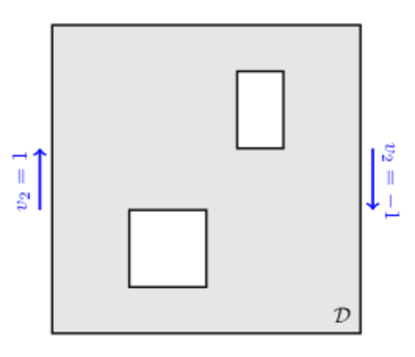
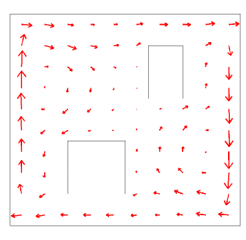
Figure 9. Left: Sketch of domain for the advective-diffusive inverse transport problem (39) showing imposed velocities used to compute the velocity field $\boldsymbol{v}$. Right: The velocity field computed from the solution of the Navier-Stokes equations and subsampled on a coarser grid for visualization purposed.

5.2.1. The noise and prior models

We consider the problem of inferring the initial condition $m$ in (39) from pointwise noisy observations $\boldsymbol{d}_{i}\in\mathbb{R}^{n_{t}}$ ($i=1,\ldots,n_{s}$) of the state $u$ at $n_{s}$ discrete time samples $t_{i}$ in interval $[T_{1},T]\subset[0,T]$, and $n_{t}$ locations in space. We assume that the observations $\boldsymbol{d}_{i}$ are perturbed with i.i.d. Gaussian additive noise with variance $\sigma^{2}$. To construct the prior, we assume a constant mean and define $\mathcal{C}_{\text{\tiny{prior}}}:=\mathcal{A}^{-2}=(-\gamma\boldsymbol{\Delta}+\delta I)^{-2}$, equipped with Robin boundary conditions $\gamma\nabla m\cdot\boldsymbol{n}+\beta m$ on $\partial\mathcal{D}$. The parameters $\gamma,\delta>0$ control the correlation length and variance of the prior operator; here we take $\gamma=1$ and $\delta=8$. The Robin coefficient $\beta$ is chosen as in (Daon and Stadler, 2018; Roininen et al., 2014) to reduce boundary artifacts.

5.2.2. The MAP point

To compute the MAP point we minimize the negative log-posterior, defined in general in (13), which—for Gaussian prior and noise—is analogous to the least-squares functional minimized in the solution of a deterministic inverse problem. For this particular problem, this reads

(41) $$\mathcal{J}(m):=\frac{1}{2\sigma^{2}}\sum_{i=1}^{n_{s}}\int_{T_{1}}^{T}(\mathcal{B}u-\boldsymbol{d}_{i})^{2}\delta_{t_{i}}\,dt+\frac{1}{2}\left\|\mathcal{A}(m-m_{\text{pr}}\right)\|^{2}_{L^{2}(\mathcal{D})},$$

where $\mathcal{B}:\mathscr{V}_{\!\scriptscriptstyle{0}}\mapsto\mathbb{R}^{n_{t}}$ is the interpolation operators at the observation locations, $\delta_{t_{i}}$ is the Dirac delta functions at the observation time sample $t=t_{i}$ ($i=1,\ldots,n_{s}$), and $\sigma^{2}$ represents the noise level in the observations $\boldsymbol{d}_{i}$, here taken $2.45\times 10^{-7}$, and $m_{\text{pr}}=0$ is the prior mean. We use the conjugate gradient method to solve this (linear) inverse problem. The derivation of the gradient and Hessian-apply is given in Appendix B.

5.2.3. Numerical results

Next, we present numerical results for the initial condition inverse problem. The discretization of the forward and adjoint problems uses an unstructured triangular mesh, Galerkin finite elements with piecewise-quadratic globally-continuous polynomials, and an implicit Euler method for the time discretization. Galerkin Least-Squares stabilization of the convective term (Hughes et al., 1989) is added to ensure stability of the discretization. The space-time dimension of the state variable is 433880 (10847 spatial degree of freedom times 40 time steps), and the dimension of the parameter space is 10847. The data dimension $q$ is 1200 with $n_{t}=80$ measurement locations and $n_{s}=15$ time samples.

To illustrate properties of the forward problem, Fig.  10 show three snapshots in time of the field $u$, using the advective velocity $\boldsymbol{v}$ from Fig.  9 with the “true” initial condition (top row) and its MAP point estimate (bottom row), respectively. Next we study the numerical rank of the prior-preconditioned data misfit Hessian. Note that due to linearity of the parameter-to-observable map $\mathcal{F}$, the prior-preconditioned data misfit Hessian is independent of $m$. Fig.  11 (left) shows a logarithmic plot of the truncated spectra of the prior-preconditioned data misfit Hessians for several observation time horizons. This plot shows that the spectrum decays rapidly and, as expected, the decay is faster when the observation time horizon is shorter (i.e., there are fewer observations). As seen in (25), an accurate low-rank based approximation of the inverse Hessian can be obtained by neglecting eigenvalues that are small compared to 1. Thus, retaining around 70 eigenvectors out of 10847 appears to be sufficient for the target problem with spatial and temporal observation points in the interval $[1,4]$. These eigenvalues and the corresponding prior-orthogonal eigenvectors (see the right panel in Fig.   11) were computed using the double pass algorithm Algorithm 2 with $r=50$ and oversampling parameter $l=10$.

Due to the linearity of the parameter-to-observable map and the choice of a Gaussian prior and noise model, the posterior distribution is also Gaussian whose mean coincides with the MAP point and the covariance with the inverse of the Hessian evaluated at the MAP point. Thus, for this problem, the Laplace approximation is the posterior distribution. Fig.  12 depicts the prior and posterior pointwise variances. This figure shows that the uncertainty is reduced everywhere in the domain, and that the reduction is greatest near to the observations (at the boundaries of the interior rectangles). In Fig.  13 we show samples (of the initial condition) from the prior and from the posterior, respectively. The difference between the two sets of samples reflects the information gained from the data in solving the inverse problem. The small differences in the parameter field $m$ across the posterior samples (other than near the external boundaries) demonstrate that there is small variability in the inferred parameters, reflecting large uncertainty reduction.

Figure 10. Forward advective-diffusive transport estimate of the inverse solution at initial time t = 0 (a, d), at t = 1 (b, e), t = 2 (c, f) and at final time t = 4 (d) with the “true” (top) and MAP (bottom) as initial conditions.

Figure 11. Left: Log-linear plot of the truncated spectrum of prior-preconditioned data misfit Hessian for observation times (sampled every 0.2 time units) in the intervals $[1,4]$ (blue), $[2,4]$ (red), and $[3,4]$ (green). The low-rank approximation captures the dominant, data-informed portion of the spectrum. The eigenvalues are truncated at around $0.06$. Right: Prior-orthogonal eigenvectors of the prior-preconditioned data misfit Hessian corresponding (from left to right) to the 1st, 4th, 7th, and 60th eigenvalues. Eigenvectors corresponding to smaller eigenvalues are increasingly more oscillatory (and thus inform smaller length scales of the initial concentration) but are also increasingly less informed by the data.

Figure 12. This figure shows the pointwise variance of the prior (left) and posterior (right) distributions.

Figure 13. Top: Prior mean initial concentration $m_{\text{pr}}$ (a), and samples drawn from the prior distribution (b)–(d). Bottom: The MAP point (e), and samples drawn from the posterior distribution (f)–(h).

6. Conclusions

We have presented an extensible software framework for large-scale deterministic and linearized Bayesian inverse problems governed by partial differential equations. The main advantage of this framework is that it exploits the structure of the underlying infinite-dimensional PDE based parameter-to-observable map, in particular the low effective dimensionality, which leads to scalable algorithms for carrying out the solution of deterministic and linearized Bayesian inverse problems. By scalable, we mean that the cost—measured in number of (linearized) forward (and adjoint) solves—is independent of the state, parameter, and data dimensions. The cost depends only on the number of modes in parameter space that are informed by the data. We have described the main algorithms implemented in hIPPYlib, namely the inexact Newton-CG method to compute the MAP point (Section 4.1), randomized eigensolvers to compute the low rank approximation of the Hessian evaluated at the MAP point (Section 4.2), and algorithms for sampling and computing the pointwise variance from large-scale Gaussian random fields (Sections 4.3 and 4.4). To illustrate their use, we applied these methods to two model problems: inversion for the log coefficient field in a Poisson equation, and inversion for the initial condition in a time-dependent advection-diffusion equation.

The contributions of our work are as follows. On the algorithm side, our framework incorporates modifications of state-of-the-art algorithms to ensure consistency with infinite-dimensional settings and a novel square-root-free implementation of the low-rank approximation of the Hessian, sampling strategies, and pointwise variance field computation. On the software side, we created a library for the solution of deterministic and linearized Bayesian inverse problems that allows researchers who are familiar with variational methods to solve inverse problems under uncertainty even without possessing expertise in all of the necessary numerical optimization and statistical aspects. Our framework provides dimension-independent algorithms for finding the maximum a posteriori (MAP) point, constructing a low-rank based approximation of the Hessian and its inverse at the MAP, sampling from the prior and posterior distributions, and computing pointwise variance fields. hIPPYlib is easily extensible, that is, if a user can express the forward problem in variational form using FEniCS, hIPPYlib effortlessly allows solving the inverse problem, exploring and testing various priors, observation operators, noise covariance models, etc.

The framework presented here relies on a second order Taylor expansion of the negative log-likelihood with respect to the uncertain parameter centered at the MAP point, which leads to the Laplace approximation of the posterior distribution. Ultimately one would like to relax this approximation and fully explore the resulting non-Gaussian distributions. Ongoing work includes the implementation of scalable, robust, Hessian-based MCMC methods capitalizing on hIPPYlib’s capabilities to build local Laplace approximations of the posterior based on gradient and Hessian information as described here.

Appendix A Gradient and Hessian actions computation for the inverse problem governed by the Poisson PDE

In what follows, we apply the technique outlined in Section 2.1 and derive expressions for the gradient and Hessian actions of the cost functional $\mathcal{J}(m)$ defined in (38). The Lagrangian functional for this optimization problem is given by

(42) $$\mathscr{L}^{\mathcal{G}}(u,m,p):=\mathcal{J}(m)+{\left\langle{e^{{m}}\nabla u},{\nabla p}\right\rangle}-{\left\langle{f},{p}\right\rangle}-{\left\langle{p},{h}\right\rangle}_{\Gamma_{\!\!N}},$$

where the last three terms stem from the variational form (36) of the forward problem (35). The formal Lagrange multiplier method (Tröltzsch, 2010) requires that, at a minimizer of (38), variations of the Lagrangian functional with respect to $p$ and $u$ vanish, which yields to solving the forward and adjoint problems

(43a) $${\left\langle{e^{{m}}\nabla u},{\nabla\tilde{p}}\right\rangle}-{\left\langle{f},{\tilde{p}}\right\rangle}-{\left\langle{\tilde{p}},{h}\right\rangle}_{\Gamma_{\!\!N}} =0,\quad\forall\tilde{p}\in\mathcal{V}_{0};$$

(43b) $${\left\langle{e^{{m}}\nabla\tilde{u}},{\nabla p}\right\rangle}+{\left\langle{\mathcal{B}^{*}\boldsymbol{\Gamma}_{\!\mbox{\tiny noise}}^{-1}(\mathcal{B}u-\boldsymbol{d})},{\tilde{u}}\right\rangle} =0,\quad\forall\tilde{u}\in\mathcal{V}_{0}.$$

The strong form of the forward problem is given in (35), while the strong form of the adjoint problem reads

(44) $$\begin{split}-\nabla\cdot(e^{{m}}\nabla p)&=\mathcal{B}^{*}\boldsymbol{\Gamma}_{\!\mbox{\tiny noise}}^{-1}(\mathcal{B}u-\boldsymbol{d})\quad\text{ in }\mathcal{D},\\ p&=0\quad\text{ on }\Gamma_{\!\!D},\\ e^{{m}}\nabla{p}\cdot\boldsymbol{n}&=0\quad\text{ on }\Gamma_{\!\!N}.\end{split}$$

Finally, the gradient of the cost functional (38) is given in weak form by

(45) $$\left(\mathcal{G}(m),\tilde{m}\right)={\left\langle{m-m_{\text{pr}}},{\tilde{m}}\right\rangle}_{\mathcal{C}_{\text{\tiny{prior}}}^{-1}}+{\left\langle{\tilde{m}e^{{m}}\nabla u},{\nabla p}\right\rangle},\quad\forall\tilde{m}\in\mathcal{M},$$

where $u$ and $p$ are solutions to the forward and adjoint problems (43a)-(43b), respectively (Tröltzsch, 2010; Borzì and Schulz, 2012). In strong form this reads

(48) $$\mathcal{G}(m)=\left\{\begin{array}[]{ll}\mathcal{C}_{\text{\tiny{prior}}}^{-1}(m-m_{\text{pr}})+e^{{m}}\left({\nabla u}\cdot{\nabla p}\right)&\text{in }\mathcal{D},\\ \gamma\left(\Theta\nabla m\right)\cdot\boldsymbol{n}+\beta m&\text{on }\partial\mathcal{D}.\end{array}\right.$$

We note that to evaluate the gradient for a given parameter $m$, one needs to solve the forward problem (43a) for $u$, and then given $m$ and $u$ solve the adjoint problem for $p$. This evaluation of the gradient costs one forward and one adjoint PDE solve.

Next, we derive the expression of the Hessian action following Section 2.1. The second order Lagrangian functional in this case reads

$$\mathscr{L}^{\mathcal{H}}(u,m,p;\hat{u},\hat{m},\hat{p}) :=\left(\mathcal{G}(m),\hat{m}\right)$$

$$+{\left\langle{e^{{m}}\nabla u},{\nabla\hat{p}}\right\rangle}-{\left\langle{f},{\hat{p}}\right\rangle}-{\left\langle{\hat{p}},{h}\right\rangle}_{\Gamma_{\!\!N}}$$

$$+{\left\langle{e^{{m}}\nabla\hat{u}},{\nabla p}\right\rangle}+{\left\langle{\mathcal{B}^{*}\boldsymbol{\Gamma}_{\!\mbox{\tiny noise}}^{-1}(\mathcal{B}u-\boldsymbol{d})},{\hat{u}}\right\rangle}.$$

To obtain the action of the Hessian in a direction $\hat{m}$ we take the variation of $\mathscr{L}^{\mathcal{H}}$ with respect to $m$, namely

(49) $$\!\left(\tilde{m},\mathcal{H}(m)\hat{m}\right) ={\left\langle{\tilde{m}e^{{m}}\nabla\hat{u}},{\nabla p}\right\rangle}\!+\!{\left\langle{\hat{m}},{\tilde{m}}\right\rangle}_{\mathcal{C}_{\text{\tiny{prior}}}^{-1}}\!$$

(50) $$+\!{\left\langle{\tilde{m}\hat{m}e^{{m}}\nabla u},{\nabla p}\right\rangle}\!+\!{\left\langle{\tilde{m}e^{{m}}\nabla u},{\nabla\hat{p}}\right\rangle},\quad\forall\tilde{m}\in\mathcal{M},$$

where as before $u$ and $p$ are the solutions of the forward and adjoint problems in (43a) and (43b), respectively, and the $\hat{u}$ and $\hat{p}$ are the solutions of the incremental forward and adjoint problems, respectively. These equations are given by

(51) $${\left\langle{e^{{m}}\nabla\hat{u}},{\nabla\tilde{p}}\right\rangle}+{\left\langle{\hat{m}e^{{m}}\nabla u},{\nabla\tilde{p}}\right\rangle}=0,\quad\forall\tilde{p}\in\mathscr{V}_{\!\scriptscriptstyle{0}},$$

and

(52) $${\left\langle{\mathcal{B}^{*}\boldsymbol{\Gamma}_{\!\mbox{\tiny noise}}^{-1}\mathcal{B}\hat{u}},{\tilde{u}}\right\rangle}+{\left\langle{\hat{m}e^{{m}}\nabla\tilde{u}},{\nabla p}\right\rangle}+{\left\langle{e^{{m}}\nabla\tilde{u}},{\nabla\hat{p}}\right\rangle}=0,\quad\forall\tilde{u}\in\mathscr{V}_{\!\scriptscriptstyle{0}}.$$

Once we have the gradient and Hessian action expressions, we can apply Algorithm 1 to solve the optimization problem given by (38).

Appendix B Gradient computation for inverse problem governed by the advection-diffusion PDE

To derive an expression for the gradient of $\mathcal{J}(m)$ in (41), we define the Lagrangian functional

$$\mathscr{L}^{\mathcal{G}}(u,m,p,p_{0}):=\mathcal{J}(m) +\int_{0}^{T}\!\int_{\mathcal{D}}(u_{t}+\boldsymbol{v}\cdot\nabla u)p\,d\boldsymbol{x}\,dt$$

$$+\int_{0}^{T}\!\int_{\mathcal{D}}\kappa\nabla u\cdot\nabla p\,d\boldsymbol{x}\,dt+\int_{\mathcal{D}}(u(\boldsymbol{x},0)-m)p_{0}\,d\boldsymbol{x},$$

where $p\in\mathcal{V}$ and $p_{0}\in\mathcal{M}$ are the Lagrangian multiplier, i.e., the adjoint variables, for, respectively, the advection-diffusion PDE and initial condition in the forward problem (39). Expressions needed to compute the gradient of (41) are obtained by setting variations of the Lagrangian $\mathscr{L}^{\mathcal{G}}$ with respect to $p$, $p_{0}$ and $u$ to zero. Variations with respect to $p$ and $p_{0}$ recover the variational form (40) of the forward problem. The variation with respect to $u$ in an arbitrary direction $\tilde{u}$ yields

$$\frac{1}{\sigma^{2}}\sum_{i=1}^{n_{s}}\int_{T_{1}}^{T}(\mathcal{B}u-\boldsymbol{d}_{i})\tilde{u}\,\delta_{t_{i}}\,dt+\int_{0}^{T}\int_{\mathcal{D}}(\tilde{u}_{t}+\boldsymbol{v}\cdot\nabla\tilde{u})p\,d\boldsymbol{x}\,dt$$

$$+\int_{0}^{T}\int_{\mathcal{D}}\kappa\nabla\tilde{u}\cdot\nabla p\,d\boldsymbol{x}\,dt+\int_{\mathcal{D}}\tilde{u}(\boldsymbol{x},0)p_{0}\,d\boldsymbol{x}=0 \quad\forall\tilde{u}\in\mathcal{V}.$$

Integration by parts in time for the term $\tilde{u}_{t}p$ and in space for $(\boldsymbol{v}\cdot\nabla\tilde{u})p$ and $\kappa\nabla\tilde{u}\cdot\nabla p$ results in

$$\frac{1}{\sigma^{2}}\sum_{i=1}^{n_{s}}\int_{T_{1}}^{T}(\mathcal{B}u -\boldsymbol{d}_{i})\tilde{u}\,\delta_{t_{i}}\,dt-\int_{0}^{T}\!\int_{\mathcal{D}}(\tilde{p}_{t}+\nabla\cdot(\boldsymbol{v}p)+\kappa\Delta p)\tilde{u}\,d\boldsymbol{x}\,dt+\int_{\mathcal{D}}\tilde{u}(\boldsymbol{x},T)p(\boldsymbol{x},T)$$

$$-\tilde{u}(\boldsymbol{x},0)p(\boldsymbol{x},0)+\tilde{u}(\boldsymbol{x},0)p_{0}\,d\boldsymbol{x}+\int_{0}^{T}\int_{\partial\mathcal{D}}(\boldsymbol{v}p+\kappa\nabla p)\cdot\boldsymbol{n}\tilde{u}\,d\boldsymbol{x}\,dt=0,$$

$\tilde{u}\in\mathcal{V}$. This implies $p_{0}=p(\boldsymbol{x},0)$ and leads to the strong form of the adjoint problem,

(53) $$-p_{t}-\nabla\cdot(p\boldsymbol{v})-\kappa\Delta p =-\frac{1}{\sigma^{2}}\mathcal{B}^{*}\sum_{i=1}^{n_{s}}\left(\mathcal{B}u-\boldsymbol{d}_{i}\right)\delta_{t_{i}} \text{ in }\mathcal{D}\times(0,T),$$

$$p(\cdot,T) =0 \text{ in }\mathcal{D},$$

$$(\boldsymbol{v}p+\kappa\nabla p)\cdot\boldsymbol{n} =0 \text{ on }\partial\mathcal{D}\times(0,T).$$

Note that (53) is a final value problem, since $p$ is specified at $t=T$ rather than at $t=0$. Thus, (53) is solved backwards in time, which amounts to the solution of an advection-diffusion equation with velocity $-\boldsymbol{v}$.

Finally, the variation of the Lagrangian with respect to the initial condition $m$ in a direction $\tilde{m}$ gives the weak form of the gradient of the cost functional $\mathcal{J}(m)$,

(54) $$\left(\mathcal{G}(m),\tilde{m}\right)=\int_{\mathcal{D}}\big{(}\mathcal{A}(m-m_{\text{pr}})\big{)}\big{(}\mathcal{A}\tilde{m}\big{)}-p(\boldsymbol{x},0)\tilde{m}\,d\boldsymbol{x},\quad\forall\tilde{m}\in\mathcal{M},$$

where we used $p_{0}=p(\boldsymbol{x},0)$. The strong form of the gradient expression then reads

(55) $$\mathcal{G}(m)=\left\{\begin{array}[]{rl}\mathcal{A}^{2}(m-m_{\text{pr}})-p(\boldsymbol{x},0)&\text{ in }\mathcal{D}\\ \gamma\nabla m\cdot\boldsymbol{n}+\beta m&\text{ in }\partial\mathcal{D}.\end{array}\right.$$

Thus, the adjoint of the parameter-to-observable map $\mathcal{F}^{*}$ is defined by setting $\mathcal{F}^{*}\boldsymbol{d}=p(\boldsymbol{x},0)$. We note that the gradient expression in (55) is linear in $m$, since $p$ depends linearly on $u$ through the solution of the adjoint problem (53), and $u$ depends linearly on $m$ through the solution of the forward problem (39). Elimination of the forward and adjoint equations for a given $m$ gives the action of the linear operator in (55) in the direction of that $m$. Thus, to compute the MAP point, we use CG to set $\mathcal{G}(m)=0$ with the inverse of the regularization operator $\mathcal{A}^{2}$ as preconditioner.

Appendix C Finite element assembly and rectangular decompositions

In this section, we describe a technique based on rectangular decompositions of finite element matrices to efficiently generate large scale samples from priors of the form described in Section 2.2. A similar approach has been also proposed in (Croci et al., 2018) to generate samples of white noise. The method described here is more general as it can be applied to matrices stemming from finite element discretization of any differential operator and not only mass matrices. More specifically, we present a finite element assembly procedure to compute a rectangular decomposition of the form

(56) $$\mathbf{{A}}=\mathbf{{C}}\mathbf{{C}}^{T},$$

for any symmetric positive definite finite element matrix $\mathbf{{A}}$. More specifically, consider the finite element assembly procedure for a generic symmetric positive definite bilinear form $a(u_{h},v_{h})$ on $\mathcal{M}_{h}$, a finite-dimensional subspace of $\mathcal{M}\subseteq L^{2}(\mathcal{D})$. The entry $(i,j)$ of the matrix $\mathbf{{A}}$, which stems from finite element discretization of the bilinear form $a(u_{h},v_{h})$, are given by

$$A_{i,j}=a\left(\phi_{i},\phi_{j}\right),\quad i,j=1,\ldots,n,$$

where $\{\phi_{i}\}_{i=1}^{n}$ is the finite element basis of the space $\mathcal{M}_{h}$. In the finite element assembly procedure we first compute the element matrices $\mathbf{{A}}_{e}$, which correspond to the restriction of the bilinear form $a$ to each element $e$ in the mesh. Then, using the global-to-local mapping of the degrees of freedom (dof) $\mathbf{{G}}_{e}$, the global matrix $\mathbf{{A}}$ is computed by summing all of the local contributions as follows:

(57) $$\mathbf{{A}}=\sum_{e}\mathbf{{G}}_{e}^{T}\mathbf{{A}}_{e}\mathbf{{G}}_{e}=\sum_{e}\mathbf{{G}}_{e}^{T}\mathbf{{B}}^{T}\mathbf{{D}}_{e}\mathbf{{B}}\mathbf{{G}}_{e}.$$

Here we have written the element matrix $\mathbf{{A}}_{e}=\mathbf{{B}}^{T}\mathbf{{D}}_{e}\mathbf{{B}}$ as the product of the element-independent dof-to-quadrature point basis evaluation matrix $\mathbf{{B}}$ and the (block) diagonal matrix $\mathbf{{D}}_{e}\in\mathbb{R}^{q\times q}$ at the quadrature points, where $q$ denotes the total number of quadrature nodes over all elements, which scales linearly with the number of elements in the mesh.
A rectangular decomposition of $\mathbf{{A}}$ can then be explicitly constructed from the matrices $\mathbf{{G}}_{e}$, $\mathbf{{B}}$, and $\mathbf{{D}}_{e}$ as follows. For each element $e$ of the mesh we define the matrix $\mathbf{{C}}_{e}=\mathbf{{G}}_{e}^{T}\mathbf{{B}}^{T}\mathbf{{D}}_{e}^{\frac{1}{2}}$. Since, for any two elements $e_{i}$ and $e_{j}$ ( $i\neq j$) in the mesh, the sets of quadrature nodes relative to the elements $e_{i}$ and $e_{j}$ are disjoint, we have that

(58) $$\mathbf{{C}}_{e_{i}}\mathbf{{C}}^{T}_{e_{j}}=\delta_{ij}\mathbf{{A}}_{e_{i}}.$$

Then the rectangular matrix $\mathbf{{C}}\in\mathbb{R}^{n\times q}$ defined as

(59) $$\mathbf{{C}}=\sum_{e}\mathbf{{G}}_{e}^{T}\mathbf{{B}}^{T}\mathbf{{D}}_{e}^{\frac{1}{2}}=\sum_{e}\mathbf{{C}}_{e}$$

satisfies (56). In fact, thanks to (58) we have

$$\mathbf{{C}}\mathbf{{C}}^{T}=\left(\sum_{e}\mathbf{{C}}_{e}\right)\left(\sum_{e}\mathbf{{C}}_{e}\right)^{T}=\sum_{e}\mathbf{{C}}_{e}\mathbf{{C}}_{e}^{T}=\sum_{e}\mathbf{{G}}_{e}^{T}\mathbf{{B}}^{T}\mathbf{{D}}_{e}\mathbf{{B}}\mathbf{{G}}_{e}=\mathbf{{A}}.$$