Drag reduction in boiling Taylor-Couette turbulence

Abstract

We create a highly controlled lab environment—accessible to both global and local monitoring—to analyse turbulent boiling flows and in particular their shear stress in a statistically stationary state. Namely, by precisely monitoring the drag of strongly turbulent Taylor-Couette flow (the flow in between two co-axially rotating cylinders, Reynolds number $\textrm{Re}\approx 10^{6}$) during its transition from non-boiling to boiling, we show that the intuitive expectation, namely that a few volume percent of vapor bubbles would correspondingly change the global drag by a few percent, is wrong. Rather, we find that for these conditions a dramatic global drag reduction of up to 45% occurs. We connect this global result to our local observations, showing that for major drag reduction the vapor bubble deformability is crucial, corresponding to Weber numbers larger than one. We compare our findings with those for turbulent flows with gas bubbles, which obey very different physics than vapor bubbles. Nonetheless, we find remarkable similarities and explain these.

1 Introduction

When the temperature of a liquid increases, the corresponding vapor pressure $P_{v}$ also increases. Once the vapor pressure equals the surrounding pressure $P_{atm}$, all of the sudden boiling starts and vapor bubbles can grow (Prosperetti, 2017; Brennen, 1995; Dhir, 1998; Theofanous et al., 2002b, a; Dhir, 2005; Nikolayev et al., 2006; Kim, 2009) (preferentially starting on nucleation sites such as on immersed microparticles), dramatically changing the characteristics of the flow (Gungor & Winterton, 1986; Weisman & Pei, 1983; Tong, 2018; Amalfi et al., 2016). Similarly, cavitation requires that the pressure is locally lowered so that it matches the vapor pressure at the given temperature, and again vapor bubbles emerge, again dramatically changing the flow characteristics (Brennen, 1995; Arndt, 2002). Both boiling and cavitation lie at the basis of a vast range of different phenomena in daily life, nature, technology, and industrial processes. For boiling, many of them are connected with energy conversion such as handling of LNGs (e.g., pumping through pipes or pipelines), liquified CO₂, riser tubes of steam generators, boiler tubes of power plants, or cooling channels of boiling water nuclear reactors. The sudden change of the global flow characteristics at the boiling point can lead to catastrophic events (Gungor & Winterton, 1986; Weisman & Pei, 1983; Tong, 2018; Amalfi et al., 2016). In nature, examples for such catastrophic events in boiling turbulent flows include volcano or geyser eruptions (Manga & Brodsky, 2006; Toramaru & Maeda, 2013). For cavitation, one example is the cavitation behind rapidly rotating ship propellors, drastically reducing the propulsion (Carlton, 2012; Geertsma et al., 2017) and another one is the occurrence of cavitating bubbles in turbomachinery, where the corresponding huge pressure fluctuations can cause major damage (d’Agostino & Salvetti, 2007). In spite of the relevance and the omnipresence of boiling and cavitation in turbulent flows, the physics governing the corresponding pressure drop and thus the reduced wall shear stress or propulsion is not fully understood, also due to the lack of controlled experiments.

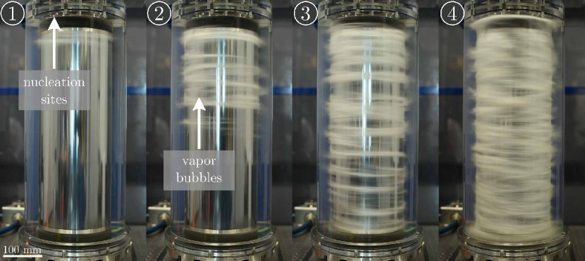
Figure 1: Vapor bubble generation and migration close to the surface of the IC in the boiling regime. Each image corresponds to a different stage during the experiment. Time moves from left to right: the numbers on top of each image corresponds to the time steps shown in figure 3d. The nucleation of vapor bubbles starts on top of the cell because the hydrostatic pressure there is smaller. The vapor bubble front then travels downwards by bubble dispersion until the surface of the IC is fully covered. Note that the volume fraction is increasing with time.

In this paper, we want to contribute to the understanding of boiling turbulent flows, by performing and analysing controlled boiling experiments in turbulent Taylor-Couette (TC) flow, i.e. the flow in between two coaxial co- or counterrotating cylinders. For a detailed overview of single-phase TC flow, we refer the reader to Grossmann et al. (2016). This flow has the unique advantage of being closed, with global balances, and no spatial transients. Also the underlying equations and boundary conditions are well-known and well-defined so that the turbulent flow is mathematically and numerically accessible. More concretely, the experiments are performed in the Boiling Twente Taylor-Couette (BTTC) facility (Huisman et al., 2015), which allows us to control and access at the same time both global and local flow quantities, namely to measure the torque $\mathcal{T}$ required to drive the cylinders at constant speed, the liquid temperature $T_{TC}$ in the cell, the pressure $P$ of the system, the volume fraction $\alpha$ of the vapor, and in the beginning of the vapor bubble nucleation process even the positions and sizes of individual vapor bubbles, all as function of time, so that we can study the dynamics and evolution of the boiling process. The focus of the work is on the onset and evolution of turbulent drag reduction induced by the nucleating vapor bubbles in the turbulent flow. We will compare it with the case of air bubbles in turbulent flow with similar turbulence level and fixed gas volume fraction. For air bubbles, van Gils et al. (2013) have shown that with a small volume fraction of only $\alpha\approx 4\%$, very large drag reduction of $\approx 40\%$ can be achieved, provided the turbulence level is high, i.e. $\mathcal{O}(\text{Re})\approx 10^{6}$. We will not only compare the drag reduction effect of vapor and gas bubbles, but also their deformabilities, which have turned out to be essential for bubbly drag reduction (Lu et al., 2005; van den Berg et al., 2005; van Gils et al., 2013; Verschoof et al., 2016; Spandan et al., 2018).

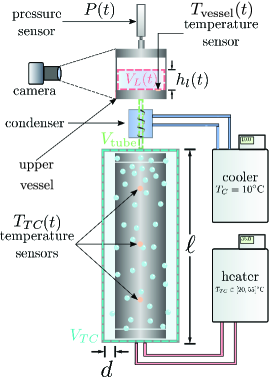
Figure 2: Diagram of the experimental apparatus. The control volume defined by the blue dashed lines corresponds to the volume of the cell $V_{TC}$. Correspondingly, in green dashed lines we highlight the volume of the tubing $V_{\text{tube}}$. Finally, in red dashed lines we highlight the volume of the liquid height in the upper vessel $V_{L}(t)$.

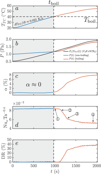
Figure 3: (a) Liquid temperature $T_{TC}$, (b) pressure $P$, c) volume fraction $\alpha$, (d) the compensated Nusselt number $\text{Nu}_{\omega}\text{Ta}^{-0.4}$, and (e) the drag reduction (DR) as a function of time. The gray shaded area and the blue lines correspond to data in the non-boiling regime, i.e. $t<t_{\text{boil}}$. The boiling point is defined using the intersection $P=P_{v}$ at a certain time as it is shown in (b). The time steps in (d) correspond to the photographs shown in figure 1.

2 Experimental setup and procedure

In order to properly measure the drag reduction and the vapor volume fraction $\alpha$ in the flow as function of time, we have extended the BTTC facility (Huisman et al., 2015) for boiling TC flow, see figure 1 for examples of vapor bubbles in the BTTC at different stages in time. In figure 2, we show a sketch of the experimental setup. The radius of the inner and outer cylinder of the BTTC are $r_{i}=$75\text{\,}\mathrm{mm}$$ and $r_{o}=$105\text{\,}\mathrm{mm}$$, respectively. The gap is then $d=r_{o}-r_{i}=$30\text{\,}\mathrm{mm}$$ and the radius ratio is $\eta=r_{i}/r_{o}=5/7=0.714$, which is very close to $\eta=0.716$ of the Twente Turbulent Taylor-Couette facility (van Gils et al., 2011a). The height of the cylinders is $\ell=$549\text{\,}\mathrm{mm}$$, which gives an aspect ratio of $\Gamma=\ell/d=18.3$. In order to allow for liquid expansion due to changes in temperature, the cell is connected to a transparent closed cylindrical container which we refer to as the upper vessel. The cell and the upper vessel are connected via plastic tubing and an aluminum heat exchanger which is in direct contact with a water liquid bath. The coil and the liquid bath forms a very efficient condenser that condenses liquid back into the cell. The cell of the BTTC, the upper vessel, and the tubing that connects them form a closed reservoir; neither liquid nor vapor can leak out of the system.

A circulator Julabo FP50-HL unit controls the temperature of the water bath for the condenser. A PT 100 temperature sensor in the upper vessel monitors the liquid temperature $T_{\text{vessel}}(t)$. Since the system is closed, the increment in temperature translates into an increment in relative pressure which we monitor with an Omega PXM409-002BGI pressure sensor. The pressure signal is then calculated as $P(t)=P_{atm}+p(t)$, where $p(t)$ is the measured relative pressure. In order to avoid a possible overpressure of the system, a $1\text{\,}\mathrm{bar}$ pressure release valve is connected to the upper vessel. We use a Nikon D300 camera to record the liquid height in the upper vessel $h_{L}(t)$ during the experiment. From this measurement, the liquid volume in the upper vessel can be calculated as $V_{\text{vessel}}(t)=\pi(D/2)^{2}h_{L}(t)$, where $D=$100\text{\,}\mathrm{mm}$$ is the inner diameter of the upper vessel. The volume $V_{vessel}(t)$ and temperature of the liquid $T_{vessel}(t)$ in the upper vessel, along with the temperature of the liquid in the cell $T_{TC}(t)$ are used to calculate the volume fraction $\alpha(t)$ during the experiments as described in detail in appendix A.

The heating of the liquid phase is done via the surface of the IC which is itself heated through channels, where hot water can flow due to a second circulator Julabo FP50-HL. The IC is made out of stainless steel. Three temperature sensors distributed along the vertical axis of the IC measure the liquid temperature during the experiment. We take the average of the three sensors to calculate the liquid temperature inside the cell $T_{TC}(t)$. A Althen 01167-051 hollow flanged reaction torque transducer (located inside the IC) measures the torque $\mathcal{T}$ required to drive the IC at constant speed. In addition to the torque experiments, we perform local measurements of the size of the vapor bubbles using high-speed imaging. The recordings were done with a Photron SA-X high-speed camera, with a frame rate of 13,500 fps. The framing of the camera results in a viewing area of $$43.5\text{\,}\mathrm{mm}$\times$43.5\text{\,}\mathrm{mm}$$ mm and it was recorded at mid-height. The focus plane of the camera is located at $(r-r_{i})/d\approx 0.9$, thus the imaged bubbles are very close to the OC. The higher density of vapor bubbles near the IC makes the detection of these bubbles less reliable than for bubbles close to the outer cylinder.

Boiling water requires liquid temperatures of $\approx$100\text{\,}\mathrm{\SIUnitSymbolCelsius}$$, which turns out to be impractical in the BTTC facility: the glass transition temperature of PMMA, from which the outer cylinder is made of, can be as low as $\approx$82\text{\,}\mathrm{\SIUnitSymbolCelsius}$$. Therefore, instead of water, we use the commercially available low boiling point Novec Engineered Fluid 7000 ($\text{C}_{3}\text{F}_{7}\text{OCH}_{3}$) liquid instead. This liquid boils at roughly $34\text{\,}\mathrm{\SIUnitSymbolCelsius}$ at atmospheric pressure. The density of the liquid $\rho_{\ell}$, its kinematic viscosity $\nu_{\ell}$, and its surface tension (air/liquid) $\sigma$ depend on temperature. These dependencies can be found in Rausch et al. (2015).

The experimental procedure is as follows: we fill the system with the low-boiling point liquid until an initial liquid height can be seen in the upper vessel. Next, we rotate the IC at a fixed rotation frequency $f_{i}=$20\text{\,}\mathrm{Hz}$$ while maintaining an initial liquid temperature of $20\text{\,}\mathrm{\SIUnitSymbolCelsius}$. Here, the ratio of centrifugal to gravitational acceleration is $a_{centr}/g=(2\pi f_{i})^{2}r_{i}/g\approx 121$. At this stage, the entire fluid is still liquid. Once the system reaches thermal equilibrium, we strongly increase the liquid temperature $T_{TC}$ in the cell within the range $T_{TC}\in[$20\text{\,}\mathrm{\SIUnitSymbolCelsius}$,$55\text{\,}\mathrm{\SIUnitSymbolCelsius}$]$. Eventually, the boiling point of the liquid is reached and we observe the nucleation of small vapor bubbles on top of the cylinder as shown in the first panel of figure 1. The nucleation of vapor bubbles starts on top of the cell because the hydrostatic pressure there is smaller. Since the nucleated vapor bubbles are small, they are carried away by the flow and are able to migrate downwards close to the surface of the IC as shown in the second panel of figure 1. Note that the effective Froude number of the vapor bubbles, i.e. the ratio of centrifugal to gravitational forces is $\text{Fr}=\sqrt{\tilde{\rho}u_{i}^{2}/((\tilde{\rho}-1)gr_{i})}\approx 0.63$, where $\tilde{\rho}=\rho_{v}/\rho_{\ell}$ is the density ratio and $\rho_{v}$ the vapor density. The bubble migration continues until the bubble front reaches the bottom plate of the BTTC (third panel of figure 1). A casual inspection of the experiment, indicates that the volume fraction of vapor increases with temperature (see the third and fourth panels of figure 1). In summary, figure 1 shows a typical boiling experiment where we highlight four different stages of the experiment in which the bubble nucleation and migration can be fully appreciated.

In figure 3a we show the temperature ramp of the liquid phase for the experiment shown in figure 1, where a heating rate of $dT_{TC}/dt\approx 0.022\ \text{K}/\text{s}$ was used. This value is calculated by applying a linear fit to the data in the range $$60\text{\,}\mathrm{s}$<t<t_{\text{boil}}$, where $60$ s is the time at which the liquid temperature is observed to increase linearly with time, and $t_{\text{boil}}$ is the time at which the liquid starts boiling. Since the system is closed, the pressure $P$ of the system increases monotonically with temperature as can be seen in figure 3b. The boiling temperature $T_{\text{boil}}$ is a function of $P$; thus, we calculate the boiling point by plotting the vapor pressure of the liquid $P_{v}$ along with $P$ as shown in figure 3b. The boiling point occurs at $t=t_{\text{boil}}$, i.e. the instant of time where $P=P_{v}$, and as a consequence $T_{\text{boil}}\equiv T_{TC}(t_{\text{boil}})$. In this manner, we define the non-boiling regime as the time interval during the experiment where the liquid experiences pure thermal expansion and no vapor is present, i.e. $t<t_{\text{boil}}$ (or equivalently $T_{TC}<T_{\text{boil}}$). This region is shaded in gray in figure 3. Conversely, we define a boiling regime, where $t\geq t_{\text{boil}}$ (or equivalently $T_{TC}\geq T_{\text{boil}}$).

As mentioned before, the amount of vapor is seen to increase as the temperature increases beyond the boiling point. This effect can be seen throughout the third and fourth panels of figure 1, where one observes more and more bubbles as time goes by. From the conservation of mass, based on the measurements of the liquid temperature $T_{\text{vessel}}$ and the liquid height $h_{L}$ in the upper vessel (see figure 2), we can compute the instantaneous volume fraction $\alpha(t)$. The results are shown in figure 3c, where we observe, indeed, that the instantaneous volume fraction $\alpha(t)$ increases monotonically until a maximum value of $\approx 8\%$ is reached at the end of the temperature ramp. The details of the calculation of $\alpha(t)$ can be found in appendix A. This calculation is self-consistent: within the non-boiling regime $\alpha\approx 0$ and $\alpha>0$ in the boiling regime. We would like to point out that no free parameters are involved in the calculation of $\alpha(t)$. It is rather remarkable that our boiling experiments yield such large and well-controlled values of the vapor volume fraction.

In order to quantify the turbulence level of the experiments, we use the Taylor number which is defined as (Eckhardt et al., 2007; Grossmann et al., 2016):

$$\text{Ta}=\left(\frac{(1+\eta)^{4}d^{2}(r_{i}+r_{o})^{2}(2\pi f_{i})^{2}}{64\eta^{2}}\right)\frac{1}{\nu(\alpha)^{2}},$$ (1)

with $\nu(\alpha)=\nu_{\ell}(1+5\alpha/2)$, i.e. including the so-called Einstein correction for the viscosity due to the presence of the dispersed phase (Einstein, 1906), $r_{i}$ and $r_{o}$ the radii of the inner and outer cylinder of the BTTC, respectively, and $\eta=r_{i}/r_{o}$ the radius ratio. The Taylor number and the Reynolds number $\text{Re}_{i}=2\pi f_{i}r_{i}d/\nu$ are related by $\text{Ta}=\frac{(1+\eta)^{6}}{64\eta^{4}}\text{Re}_{i}^{2}$.

The response of the system, the torque or equivalently the angular velocity transfer, can—in analogy to the heat transfer in Rayleigh-Bénard flow—best be expressed in dimensionless form as the so-called generalized Nusselt number (Eckhardt et al., 2007)

$$\text{Nu}_{\omega}=\left(\frac{r_{o}^{2}-r_{i}^{2}}{8\pi^{2}\ell_{\text{eff}}r_{i}^{2}r_{o}^{2}f_{i}}\right)\frac{\mathcal{T}}{\rho(\alpha)\nu(\alpha)},$$ (2)

where $\ell_{\text{eff}}=$489\text{\,}\mathrm{mm}$$ is the effective length along the cylinder where the torque is measured, and $\rho(\alpha)=\rho_{\ell}(1-\alpha)+\rho_{v}\alpha$ is the effective density of the medium. In the ultimate regime of TC turbulence (Grossmann et al., 2016), where both the bulk and the boundary layers are turbulent ($\text{Ta}>3\times 10^{8}$), it was found that $\text{Nu}_{\omega}\propto\text{Ta}^{0.4}$ (Paoletti & Lathrop, 2011; van Gils et al., 2011b; Huisman et al., 2012, 2014). In our experiments, Ta is of the order $\mathcal{O}(10^{12})$ and thus the compensated quantity $\text{Nu}_{\omega}\text{Ta}^{-0.4}$ can be used as a measure to characterize the amount of drag reduction. In figure 3d, we show that indeed $\text{Nu}_{\omega}\propto\text{Ta}^{0.4}$ during the experiment, up to a dramatic drop some time after the boiling point is reached. In the absence of a dispersed phase (non-boiling regime), $\text{Nu}_{\omega}\text{Ta}^{-0.4}$ should remain constant because the driving strength (i.e., the angular velocity $2\pi r_{i}f_{i}$ of the inner cylinder) is fixed and all the temperature-dependent quantities are contained in both $\text{Nu}_{\omega}$ and Ta (see figure 3d). Then, in the boiling regime, the occurrence of the vapor bubbles modifies the local angular velocity flow near the IC, causing a dramatic drop in the transport of momentum (Nusselt number) (van Gils et al., 2011b), which we directly observe as a drop in the global torque. This is the signature of drag reduction in the flow, shown in figure 3e. Notice how the start of the drop in the compensated Nusselt number and the corresponding drag reduction occur at a time after the boiling point is reached. This is simply because a certain amount of time (determined by turbulent diffusion) is needed for the vapor bubbles to migrate downwards and cover the entire surface of the IC. In the context of bubbly-induced drag reduction flow, transients in the wall shear stress are known to exist. The numerical study of Xu et al. (2002) has shown for example, that in channel flow ($\text{Re}=3000$) and for air bubbles injected along the streamwise direction ($\approx 8\%$), the transients of shear stress are a function of the bubble size, i.e. larger bubbles produce higher transients. In our experiments, however, the Reynolds number is 3 decades larger ($\mathcal{O}(10^{6})$) and it is known that transients are minor and that the flow quickly adjusts to the cylinder speed because of the strong convection of momentum by the turbulence (van Gils et al., 2011a). In addition, boiling experiments were conducted with different heating rates, where no discernible differences in the DR results were observed. In other words, the time-dependent DR shown in figure 3e for $t_{\text{boil}}<t<1250$ (first, second, and third panels of figure 1) is mainly a consequence of the vapor bubbles axially redistributing along the IC.

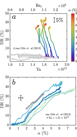
Figure 4: (a) Drag reduction DR as a function of Ta and $\alpha$ for different experiments. Note that neither $\alpha$, nor DR, nor Ta are control parameters, but responses of the system to the temperature change. The horizontal axis on top of the figure represents the Reynolds number $\text{Re}_{i}$. The color bar represents the volume fraction $\alpha$. The gray data points correspond to data in the non-boiling regime ($\text{DR}\approx 0$, $\alpha\approx 0$). The open circles represent the drag reduction obtained with air bubbles at a fixed $\text{Ta}=1.51\times 10^{12}$ (van Gils et al., 2013). A 5% error bar is shown that applies to all experiments. (b) DR as a function of the volume fraction $\alpha$. The colored lines represent the different experiments as shown in (a). The open circles correspond to the data of van Gils et al. (2013) for drag reduction using air bubbles. The error bars for both quantities DR (5%) and $\alpha$ (0.5%) are included. A 3D animation of the data is included in the supplementary material. Note the degree of reproducibility of our controlled experiments, which is remarkable for the boiling process, which is considered to be random and irregular.

3 Quantifying the drag reduction

We quantify the level of drag reduction DR through

$$\textrm{DR}=1-\frac{\textrm{Nu}_{\omega}\textrm{Ta}^{-0.4}}{\textrm{Nu}_{\omega}\textrm{Ta}^{-0.4}(t=t_{\textrm{boil}})},$$ (3)

where $\text{Nu}_{\omega}\text{Ta}^{-0.4}(t=t_{\text{boil}})$ is the compensated Nusselt number evaluated at the boiling point, where the system is still in a single phase state. In this way, $\text{DR}>0$ corresponds to a finite amount of drag reduction (boiling regime), while $\text{DR}=0$ corresponds to zero drag reduction (non-boiling regime). We note that by introducing the correction for both the viscosity $\nu(\alpha)$ and density $\rho(\alpha)$ due to the presence of the dispersed phase, the net value of DR changes slightly as compared to the case when the correction is not used. In this study—as it also done in other studies of air bubble induced DR (van Gils et al., 2013; Verschoof et al., 2016)—we set $\nu=\nu_{\ell}(1+5\alpha/2)$ and $\rho=\rho_{\ell}(1-\alpha)+\rho_{v}\alpha$ in order to draw accurate comparisons between our experiments with vapor and the case of air bubble injection. Note that by introducing these corrections to the viscosity and density (via $\alpha$), the trivial effect of drag reduction due to the density decrease of the liquid-vapor mixture is already taken into account. In figure 4a, we show DR as function of Ta and $\alpha$ for the experiment described in figures 1 and 3 along with five other experiments we performed, which confirm the reproducibility of our controlled experiments. Figures 4ab unambiguously reveal that drag reductions approaching 45% can be achieved in the boiling regime, with vapor bubbles as dispersed phase, with a volume fraction only up to 6–8%. An error bar of 5% for DR and 0.5% for $\alpha$ have been added to figures 4ab. These error bars were obtained from the repeatibility of the experiments.

Note that Ta is a non-monotonic function in the boiling regime due to the vapor fraction correction of the liquid viscosity. The reason is that when the boiling regime is reached, $\alpha$ increases at a faster rate than the rate at which $\nu_{\ell}$ decreases; and as a consequence the corrected viscosity $\nu$ increases which leads to a decrease of Ta (see equation 1). However, this effect is not significant. The converse takes place at the final stage of the experiment (see figure 3c), when $\alpha$ saturates to a certain value and as a consequence the corrected viscosity $\nu$ decreases which leads to an increment of Ta (see figure 4a). A 3D representation of figure 4 which shows the instantaneous drag reduction as a function of both Ta and $\alpha$ can be found in the supplementary movie section.

In figure 4b we show the DR as a function of the volume fraction $\alpha$, for all the corresponding experiments shown in figure 4a. This figure reveals the amount of instantaneous drag reduction that can be achieved for given vapor fraction $\alpha$ at that instant. Again, it is remarkable that with only 6 - 8% vapor bubble fraction drag reduction of nearly 45% can be achieved. This resembles the large drag reduction of up to 40% achieved by the injection of only 4% volume fraction of air bubbles into the TC system (van Gils et al., 2013).

4 Comparison to drag reduction with gas bubbles

We will now compare in more detail, the drag reduction achieved in boiling turbulent flow (vapor bubbles) with the well-known effect of drag reduction in turbulent flow with gas bubbles (Madavan et al., 1984, 1985; Merkle & Deutsch, 1992; Deutsch et al., 2004; K. et al., 2004; Lu et al., 2005; van den Berg et al., 2005; Sanders et al., 2006; van der Berg et al., 2007; Murai et al., 2008; Ceccio, 2010; Murai, 2014; Elbing et al., 2013; van Gils et al., 2013; Kumagai et al., 2015; Verschoof et al., 2016). Vapor and gas bubbles are fundamentally different (Prosperetti, 2017). While the creation, growth, and stability of gas bubbles is entirely controlled by mass diffusion, vapor bubbles are controlled by the heat diffusion and by phase transitions. For typical flows, the ratio of the heat diffusion constant and the mass diffusion constant is $k_{\ell}/D_{\ell}=\mathcal{O}(100)$. Since the surface tension in a vapor bubble is temperature-dependent, thermal Marangoni flows can further affect the vapor bubble dynamics. Given these major differences between vapor and gas bubbles, one wonders whether these major differences also reflect in different bubbly drag reduction behavior.

The answer can be read off figures 4ab, in which we have also included the drag reduction data of van Gils et al. (2013), which correspond to the case of air bubbles at a fixed $\text{Ta}=1.51\times 10^{12}$. The inspection of this figure reveals, strikingly, that both vapor and air bubbles produce a comparable amount of drag reduction when $\alpha$ and Ta are approximately the same for the two cases. Note that in gas bubble injection experiments, the gas volume fraction $\alpha$ is a control parameter, whereas in the boiling experiments, the vapor volume fraction $\alpha$ is a response of the system to the temperature increase. Indeed, for an equivalent Ta, the same amount of very large drag reduction can be obtained by either vapor or gas bubbles, given that their volume fraction is the same.

5 Bubble deformability

To achieve large drag reduction in high-Re flows with relative small gas bubble volume fraction, the gas bubble deformability has been identified as one of the crucial ingredients. This view is supported by experimental and numerical studies in high Reynolds number TC flows and other turbulent canonical flows: (Merkle & Deutsch, 1992; Moriguchi & Kato, 2002; van den Berg et al., 2005; Lu et al., 2005; Shen et al., 2006; van der Berg et al., 2007; Murai et al., 2008; van Gils et al., 2013; Murai, 2014; Verschoof et al., 2016; Rosenberg et al., 2016; Spandan et al., 2018) Whether a bubble is deformable or not is determined by the corresponding Weber number which compares inertial and capillary forces, and it also influences the mobility of the bubbles. It is defined as

$$\text{We}=\frac{\rho_{\ell}u_{\theta}^{\prime 2}d_{b}}{\sigma},$$ (4)

where $d_{b}$ is the typical bubble size, $u_{\theta}^{\prime 2}$ is the variance of the azimuthal velocity, $\sigma$ is the surface tension of the liquid/air interface. A large Weber number $\text{We}>1$ implies that the bubble is deformable. Indeed, Verschoof et al. (2016) showed that for fixed gas volume fraction $\alpha\approx 4\%$ and fixed large Reynolds number, the large drag reduction ($\approx 40\%$) could basically be “turned off” by adding a surfactant, which hinders bubble coalescence and leads to much smaller bubbles with $\text{We}<1$ in the strongly turbulent flow.

To obtain the Weber numbers of the vapor bubbles in our boiling experiments, we performed high-speed image recordings to measure the bubble size and shape. With this information at hand, we calculate the distribution of the Weber number for different volume fractions during the experiment. The velocity fluctuations $u_{\theta}^{\prime}$ (required to calculate We) as function of Ta are given by $u_{\theta}^{\prime}=11.3\times 10^{-2}(\nu_{\ell}/d)\text{Ta}^{0.44}$, as measured earlier in the same BTTC facility (Ezeta et al., 2018). The temperature variation during a high-speed measurement is $<$0.3\text{\,}\mathrm{K}$$. Therefore, all the values of the quantities in equation 4 (except for $d_{b}$) are taken as the temperature-dependent value at the beginning of each recording.

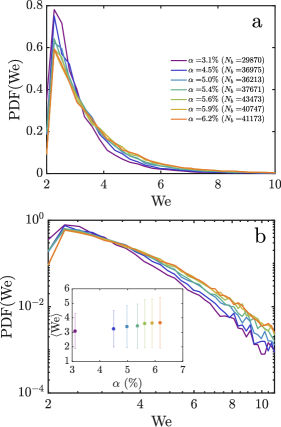
Figure 5: (a) Probability density function of the bubble Weber number during the boiling experiment for different volume fractions in linear scale. The colors represent the variation of $\alpha$ as shown in the legend. $N_{b}$ is the number of detected bubbles in every measurement. (b) Same as in (a) but in log-log scale. The inset in (b) represents the mean Weber number as function of the volume fraction. The error bars in (b) correspond to $\pm\sigma(\text{We})$, where $\sigma(\text{We})$ is the standard deviation of the Weber number for a given $\alpha$.

In figure 5, we show the probability density function (PDF) and the mean value of the Weber number for different $\alpha$ during a typical experiment in the boiling regime. These distributions reveal that $\text{We}>1$, independent of the volume fraction, i.e. the vapor bubbles in our experiments are deformable, which supports the idea that also for vapor bubbles deformability is key for achieving large drag reduction, just as shown for bubbly drag reduction with gas bubbles (van Gils et al., 2013; Verschoof et al., 2016). Moreover, we find that the maximum of all distributions lies at $\text{We}\approx 2.5$, which corresponds to bubbles of size $\approx 0.27\ \text{mm}$. The tail of every PDF extends up to $\text{We}\approx 8$, which indicates that some of the bubbles are highly deformable. Furthermore, the inset in figure 5b reveals that in the range of the volume fraction explored with the high-speed image experiments ($\alpha\in[3.1\%,6.2\%]$), the mean Weber number $\langle\text{We}\rangle$ slightly increases, namely from a value of $\langle\text{We}\rangle\approx 3.1$ to $\langle\text{We}\rangle\approx 3.7$. Notice also that as the volume fraction increases, the probability to find a larger value of We is also larger for $\text{We}>3.5$, which indicates that the deformability of the vapor bubbles increases when the number of bubbles is increased. Since the variation of $\rho_{\ell}u_{\theta}^{\prime 2}/\sigma$ is very small throughout the boiling regime ($\approx 7\%$), this shows that with increasing volume fraction it is more likely to find bigger bubbles. This can also be seen at the other tail of the distribution for values of $\text{We}<3.5$, where the probability decreases with increasing volume fraction. So when advancing the boiling process, the emerging extra vapor manifests itself in larger vapor bubbles, be it by growth or coalescence, and not in more freshly nucleated small bubbles.

6 Conclusions and Outlook

We have investigated the transport properties (i.e., the drag) of strongly turbulent boiling flow with increasing temperature in the highly controlled BTTC setup and correlated them with the vapor bubble fraction and the vapor bubble characteristics. Our highly reproducible and controlled findings reveal a sudden and dramatic drag reduction at the onset of boiling and that the emerging vapor bubbles are similarly efficient in drag reduction as injected air bubbles: Nearly 45% drag reduction can be achieved with a volume fraction of about $\approx 6\%$. In both cases the main reason for the drag reduction lies in the bubble deformability, reflected in large We $>1$. Furthermore, at later stages of the boiling process when the vapor fraction is higher, on average the bubbles are also bigger. This seems to be in line with our daily life experience when watching tea-water boil. However, this realization is not obvious since the enhanced vapor fraction could also manifest itself in smaller, freshly-nucleated bubbles.

In our experiments (figure 3a), the temperature increase is relatively modest, both in absolute numbers beyond the boiling temperature and in rate, due to experimental limitations. Furthermore, the drag reduction effect is spatially smeared out, as we measure the global drag of the whole cylinder. Nonetheless, within minutes the overall drag of the system reduces by a factor of 2. Within industrial devices, such as riser tubes of steam generators, boiler tubes of power plants, coolant channels of boiling water nuclear reactors, or when handling liquefied natural gases (LNGs) and liquefied CO₂, such sudden and large drag change can have dramatic consequences. In our experiments, the time scale of the sudden drag is determined by the heating rate and by the turbulent mixing of the emerging bubbles over the whole measurement volume. For larger heating rate and smaller volume, the rate of the drag change will be even more dramatic. Our experiments give guidelines on how to explore such events in a controlled and reproducible way.

Supplementary movies

Supplementary movies are available

Appendix A. Calculation of the volume fraction $\alpha$

We calculate dynamically the volume fraction $\alpha(t)$ using the following conservation of mass argument. At the beginning of the experiment, i.e. the start of the temperature ramp, the temperature is $T(t_{0})=T_{0}$. At this stage, the initial mass $m_{0}$ is composed only of the liquid mass which is known a priori. This is $m_{0}=\rho_{\ell}(T_{0})(V_{TC}+V_{\text{tube}}+V_{\text{vessel}}(t=t_{0}))$, where $\rho_{\ell}$ is the liquid density of the $\text{C}_{3}\text{F}_{7}\text{OCH}_{3}$, $V_{TC}$ is the volume of the BTTC cell, $V_{\text{tube}}$ is the volume that corresponds to the tubing that connects the cell to the upper vessel and $V_{\text{vessel}}(t=t_{0})$ is the liquid volume inside the upper vessel. Once the temperature ramp starts, the liquid experiences thermal expansion. This leads to a redistribution of the initial mass into $V_{TC}$, $V_{\text{tube}}$ and $V_{\text{vessel}}$ (see figure 2):

$$m_{0} = m_{TC}$$

$$+ \rho_{\ell}(T_{\text{vessel}}(t))V_{\text{tube}}+\rho_{\ell}(T_{\text{vessel}}(t))V_{\text{vessel}}(t),$$

where $m_{TC}$ is the mass inside the cell and $T_{\text{vessel}}(t)$ the temperature measured in the upper vessel, which we also assume is the temperature that corresponds to the tubing. Note that the only time dependent volume is $V_{\text{vessel}}(t)$. As the temperature $T_{TC}$ increases, the boiling point $T_{boil}$ is eventually reached and vapor bubbles start nucleating. At this stage, the mass inside the cell $m_{TC}$ is a mixture of both the liquid and the vapor phase i.e.

$$m_{TC}=\rho_{\ell}(T_{TC}(t))V_{\ell}(t)+\rho_{v}(T_{TC}(t),P(t))V_{v}(t),$$ (6)

where $T_{TC}$ is the measured temperature inside the cell, $V_{\ell}(t)$ is the volume occupied by the liquid inside the cell and $V_{v}(t)$ is the volume occupied by the vapor inside inside the cell, i.e. $V_{\ell}(t)+V_{v}(t)=V_{TC}$. The vapor density denoted by $\rho_{v}$ in equation 6 is dependent on both temperature and pressure due to the natural compressibility of the vapor phase. The vapor density is calculated by using tabulated values (Rausch et al., 2015) of $\rho_{v}(T,P_{\text{atm}})$ and assuming that the vapor experiences adiabatic expansion such that $\rho_{v}(T,P)=(P/P_{\text{atm}})\rho_{v}(T,P_{\text{atm}})$. In the absence of vapor, i.e. $\alpha=0$, $V_{v}(t<t_{boil})=0$. Using Eqs. Appendix A. Calculation of the volume fraction $\alpha$ and 6, along with the definition of the volume fraction $\alpha=V_{v}/V_{TC}$ and using that $1-\alpha=V_{\ell}/V_{TC}$, we find that

$$\alpha(t)=\frac{1-\frac{m_{0}}{\rho_{\ell}(T_{TC}(t))V_{TC}}+\frac{\rho_{\ell}(T_{\text{vessel}}(t))}{\rho_{\ell}(T_{TC}(t))}\left(\frac{V_{\text{tube}}+V_{\text{vessel}}(t)}{V_{TC}}\right)}{1-\frac{\rho_{v}(T_{TC}(t),P(t))}{\rho_{\ell}(T_{TC}(t))}}.$$ (7)

Note the spaces between the initials

References

- Amalfi et al. (2016) Amalfi, R. L., Vakili-Farahani, F. & Thome, J. R. 2016 Flow boiling and frictional pressure gradients in plate heat exchangers. part 2: Comparison of literature methods to database and new prediction methods. Int. J. Refrigeration 61, 185–203.
- Arndt (2002) Arndt, R. E. A. 2002 Cavitation in vortical flows. Annu. Rev. Fluid Mech. 34, 143–175.
- van der Berg et al. (2007) van der Berg, T.H., van Gils, D.P.M., Lathrop, D.P. & Lohse, D. 2007 Bubbly turbulent drag reduction is a boundary layer effect. Phys. Rev. Lett. 98, 084501.
- van den Berg et al. (2005) van den Berg, T. H., Luther, S., Lathrop, D. P. & Lohse, D. 2005 Drag reduction in bubbly taylor-couette turbulence. Phys. Rev. Lett. 94, 044501.
- Brennen (1995) Brennen, C. E. 1995 Cavitation and bubble dynamics. : Oxford University Press.
- Carlton (2012) Carlton, J. 2012 Marine propellers and propulsion. : Butterworth-Heinemann.
- Ceccio (2010) Ceccio, S. L. 2010 Friction drag reduction of external flows with bubble and gas injection. Annu. Rev. Fluid Mech. 42, 183–203.
- d’Agostino & Salvetti (2007) d’Agostino, L. & Salvetti, M. V. 2007 Fluid dynamics of cavitation and cavitating turbopumps. Springer-Verlag Wien.
- Deutsch et al. (2004) Deutsch, S., Moeny, M., Fontaine, A. A. & Petrie, H. 2004 Microbubble drag reduction in rough walled turbulent boundary layers with comparison against polymer drag reduction. Exp. in Fluids 37, 731–744.
- Dhir (1998) Dhir, V. K. 1998 Boiling heat transfer. Annu. Rev. Fluid Mech. 30, 365–401.
- Dhir (2005) Dhir, V. K. 2005 Mechanistic prediction of nucleate boiling heat transfer-achievable or a hopeless task? J. Heat Transfer 128, 1–12.
- Eckhardt et al. (2007) Eckhardt, B., Grossmann, S. & Lohse, D. 2007 Torque scaling in turbulent Taylor–Couette flow between independently rotating cylinders. J. Fluid Mech. 581, 221–250.
- Einstein (1906) Einstein, A. 1906 Eine neue Bestimmung der Moleküldimensionen. Ann. Phys. 324, 289–306.
- Elbing et al. (2013) Elbing, B. R., Mäkiharju, S., Wiggins, A., Perlin, M., Dowling, D. R. & Ceccio, S. L. 2013 On the scaling of air layer drag reduction. J. Fluid Mech. 717, 484–513.
- Ezeta et al. (2018) Ezeta, R., Huisman, S. G., Lohse, D. & Sun, C. 2018 Turbulent strength in ultimate Taylor-Couette flow. J. Fluid Mech. 836, 397–412.
- Geertsma et al. (2017) Geertsma, R. D., Negenborn, R. R., Visser, K. & Hopman, J. J. 2017 Design and control of hybrid power and propulsion systems for smart ships: A review of developments. Applied Energy 194, 30–54.
- van Gils et al. (2011a) van Gils, D. P. M., Bruggert, G.-W., Lathrop, D. P., Sun, C. & Lohse, D. 2011a The Twente Taylor-Couette () facility: Strongly turbulent (multiphase) flow between two independently rotating cylinders. Rev. Sci. Instrum. 82, 025105.
- van Gils et al. (2011b) van Gils, D. P. M., Huisman, S. G., Bruggert, G.-W., Sun, C. & Lohse, D. 2011b Torque scaling in turbulent Taylor-Couette flow with co- and counterrotating cylinders. Phys. Rev. Lett. 106, 024502.
- van Gils et al. (2013) van Gils, D. P. M., Narezo, D., Sun, C. & Lohse, D. 2013 The importance of bubble deformability for strong drag reduction in bubbly turbulent Taylor-Couette flow. J. Fluid Mech. 722, 317–347.
- Grossmann et al. (2016) Grossmann, S., Lohse, D. & Sun, C. 2016 High-Reynolds number Taylor-Couette turbulence. Annu. Rev. Fluid Mech. 48, 53–80.
- Gungor & Winterton (1986) Gungor, K. E. & Winterton, R. H. S. 1986 A general correlation for flow boiling in tubes and annuli. Int. J. Heat and Mass Transf. 29 (3), 351–358.
- Huisman et al. (2012) Huisman, S. G., van Gils, D. P. M., Grossmann, S., Sun, C. & Lohse, D. 2012 Ultimate turbulent Taylor-Couette flow. Phys. Rev. Lett. 108, 024501.
- Huisman et al. (2015) Huisman, S. G., van der Veen, R. C. A., Bruggert, G.-W., Lohse, D. & Sun, C. 2015 The boiling Twente Taylor-Couette (BTTC) facility: Temperature controlled turbulent flow between independently rotating, coaxial cylinders. Rev. Sci. Instrum. 86, 065108.
- Huisman et al. (2014) Huisman, S. G., van der Veen, R. C. A., Sun, C. & Lohse, D. 2014 Multiple states in highly turbulent Taylor-Couette flow. Nat. Commun. 5, 3820.
- K. et al. (2004) K., Sugiyama, Kawamura, T., Takagi, S. & Matsumoto, Y. 2004 The Reynolds number effect on the microbubble drag reduction. In Proceedings of the 5th symposium on smart conrol of turbulence, pp. 31–43. : .
- Kim (2009) Kim, J. 2009 Review of nucleate pool boiling bubble heat transfer mechanisms. Int. J. Multiph. Flow 35, 1067–1076.
- Kumagai et al. (2015) Kumagai, I., Takahashi, Y. & Murai, Y. 2015 Power-saving device for air bubble generation using a hydrofoil to reduce ship drag: Theory, experiments, and application to ships. Ocean Eng. 95, 183–194.
- Lu et al. (2005) Lu, J., Fernández, A. & Tryggvason, G. 2005 The effect of bubbles on the wall drag in a turbulent channel flow. Phys. Fluids 17, 095102.
- Madavan et al. (1984) Madavan, N. K., Deutsch, S. & Merkle, C. L. 1984 Reduction of turbulent skin friction by micro-bubbles. Phys. Fluids 27, 356.
- Madavan et al. (1985) Madavan, N. K., Deutsch, S. & Merkle, C. L. 1985 Measurements of local skin friction in a microbubble-modified turbulent boundary layer. J. Fluid Mech. 156, 237–256.
- Manga & Brodsky (2006) Manga, M. & Brodsky, E. 2006 Seismic triggering of eruptions in the far field: Volcanoes and geysers. Annu. Rev. Earth Planet. Sci 34, 263–291.
- Merkle & Deutsch (1992) Merkle, C. L. & Deutsch, S. 1992 Microbubble drag reduction in liquid turbulent boundary layers. Appl. Mech. Rev. 45, 103–127.
- Moriguchi & Kato (2002) Moriguchi, Y. & Kato, H. 2002 Influence of microbubble diameter and distribution on frictional resistance reduction. J. Mar. Sci. Technol. 7, 79–85.
- Murai (2014) Murai, Yuichi 2014 Frictional drag reduction by bubble injection. Exp. Fluids 55 (7), 1773.
- Murai et al. (2008) Murai, Y., Oiwa, H. & Takeda, Y. 2008 Frictional drag reduction in bubbly Couette-Taylor flow. Phys. Fluids 20, 034101.
- Nikolayev et al. (2006) Nikolayev, V. S., Chtain, D., Garrabos, Y. & Beysens, D. 2006 Experimental evidence of the vapor recoil mechanism in the boiling crisis. Phys. Rev. Lett. 97, 184503.
- Paoletti & Lathrop (2011) Paoletti, M. S. & Lathrop, D. P. 2011 Angular momentum transport in turbulent flow between independently rotating cylinders. Phys. Rev. Lett. 106, 024501.
- Prosperetti (2017) Prosperetti, A. 2017 Vapor bubbles. Annu. Rev. Fluid Mech. 49, 221–248.
- Rausch et al. (2015) Rausch, M. H., Kretschmer, L., Will, S., Leipertz, A. & Fröba, A.P. 2015 Density, surface tension, and kinematic viscosity of hydrofluoroethers HFE-7000, HFE-7100, HFE-7200, HFE-7300, and HFE-7500. J. Chem. Eng. Data 60, 3759–3765.
- Rosenberg et al. (2016) Rosenberg, B. J., van Buren, T., Fu, M. K. & Smits, A. J. 2016 Turbulent drag reduction over air- and liquid- impregnated surfaces. Phys. Fluids 28, 015103.
- Sanders et al. (2006) Sanders, W. C., Winkel, E. S., Dowling, D. R., Perlin, M. & Ceccio, S. L. 2006 Bubble friction drag reduction in a high-reynolds-number flat-plate turbulent boundary layer. J. Fluid Mech. 552, 353–380.
- Shen et al. (2006) Shen, X., Ceccio, S. L. & Perlin, M. 2006 Influence of bubble size on micro-bubble drag reduction. Exp. Fluids 41, 415–424.
- Spandan et al. (2018) Spandan, V., Verzicco, R. & Lohse, D. 2018 Physical mechanisms governing drag reduction in turbulent Taylor-Couette flow with finite-size deformable bubbles. J. Fluid Mech. 849, R3.
- Theofanous et al. (2002a) Theofanous, T. G., Dinh, T. N., Tu, J. P. & Dinh, A. T. 2002a The boiling crisis phenomenon - part II: Dryout dynamics and burnout. Exp. Therm. Fluid Sci. 26, 793–810.
- Theofanous et al. (2002b) Theofanous, T. G., Tu, J. P., Dinh, A. T. & Dinh, T. N. 2002b The boiling crisis phenomenon - part I: Nucleation and nucleate boiling heat transfer. Exp. Therm. Fluid Sci. 26, 775–792.
- Tong (2018) Tong, L. S. 2018 Boiling heat transfer and two-phase flow. : Routledge.
- Toramaru & Maeda (2013) Toramaru, Atsushi & Maeda, Kazuki 2013 Mass and style of eruptions in experimental geysers. J. Volcanology and Geothermal Research 257, 227–239.
- Verschoof et al. (2016) Verschoof, R.A., van der Veen, R. C. A., Sun, C. & Lohse, D. 2016 Bubble drag reduction requieres large bubbles. Phys. Rev. Lett. 117, 104502.
- Weisman & Pei (1983) Weisman, J & Pei, B. S. 1983 Prediction of critical heat flux in flow boiling at low qualities. Int. J. Heat and Mass Transf. 26 (10), 1463–1477.
- Xu et al. (2002) Xu, J., Maxey, M. R. & G., Karniadakis 2002 Numerical simulation of turbulent drag reduction using micro-bubbles. J. Fluid Mech. .