Abstract.

Deep learning has achieved overwhelming success, spanning from discriminative models to generative models. In particular, deep generative models have facilitated a new level of performance in a myriad of areas, ranging from media manipulation to sanitized dataset generation. Despite the great success, the potential risks of privacy breach caused by generative models have not been analyzed systematically. In this paper, we focus on membership inference attack against deep generative models that reveals information about the training data used for victim models. Specifically, we present the first taxonomy of membership inference attacks, encompassing not only existing attacks but also our novel ones. In addition, we propose the first generic attack model that can be instantiated in a large range of settings and is applicable to various kinds of deep generative models. Moreover, we provide a theoretically grounded attack calibration technique, which consistently boosts the attack performance in all cases, across different attack settings, data modalities, and training configurations. We complement the systematic analysis of attack performance by a comprehensive experimental study, that investigates the effectiveness of various attacks w.r.t. model type and training configurations, over three diverse application scenarios (i.e., images, medical data, and location data).

1. Introduction

Over the last few years, two categories of deep learning techniques have made tremendous progress. The discriminative model has been successfully adopted in various prediction tasks, such as image classification (Krizhevsky et al., 2012; Simonyan and Zisserman, 2015; Szegedy et al., 2015; He et al., 2016) and speech recognition (Hinton et al., 2012; Graves et al., 2013). The generative model, on the other hand, has also gained increasing attention and has delivered appealing applications including photorealistic image synthesis (Goodfellow et al., 2014; Li and Wand, 2016; Pathak et al., 2016; Yu et al., 2019), text and sound generation (Vinyals et al., 2015; Arora et al., 2017; van den Oord et al., 2016; Mehri et al., 2017), sanitized dataset generation (Beaulieu-Jones et al., 2019; Acs et al., 2017; Zhang et al., 2018b; Xie et al., 2018; Jordon et al., 2019), etc. Most of such applications are supported by deep generative models, e.g., the generative adversarial networks (GANs) (Goodfellow et al., 2014; Radford et al., 2015; Salimans et al., 2016; Arjovsky et al., 2017; Gulrajani et al., 2017; Karras et al., 2018; Brock et al., 2019; Karras et al., 2019; Karras et al., 2020; Yu et al., 2020) and variational autoencoder (VAE) (Kingma and Welling, 2014; Rezende et al., 2014; Yan et al., 2016).

In line with the growing trend of deep learning in real business, many companies collect and process customer data which is then used to develop deep learning models for commercial use. However, data privacy violations frequently happened due to data misuse with an inappropriate legal basis, e.g., the misuse of National Health Service data in the DeepMind project. Data privacy can also be challenged by malicious users who intend to infer the original training data. The resulting privacy breach would raise serious issues as training data contains sensitive attributes such as diagnosis and income. One such attack is membership inference attack (MIA) (Dwork et al., 2015; Backes et al., 2016; Shokri et al., 2017; Hagestedt et al., 2019; Hayes et al., 2019; Salem et al., 2019) which aims to identify if a data record was used to train a machine learning model. Overfitting is the major cause for the feasibility of MIA, as the learned model tends to memorize training inputs and perform better on them.

While numerous literature is dedicated to MIA against discriminative models (Shokri et al., 2017; Long et al., 2018; Yeom et al., 2018; Salem et al., 2019; Melis et al., 2019; Jia et al., 2019; Li and Zhang, 2020), the attack on generative models has not received equal attention, despite its practical importance. For instance, GANs have been applied to health record data and medical images (Choi et al., 2018; Frid-Adar et al., 2018; Yi et al., 2019) whose membership is sensitive as it may reveal a patient’s disease history. Moreover, recent works in privacy preserving data sharing (Beaulieu-Jones et al., 2019; Acs et al., 2017; Zhang et al., 2018b; Xie et al., 2018; Jordon et al., 2019; Chen et al., 2020) propose to impose (membership) privacy constraints during GANs training for sanitized data generation. Understanding the membership privacy leakage under a practical threat model helps shed light on future research in this area.

Nevertheless, this is a highly challenging task from the adversary side. Unlike discriminative models, the victim generative models do not directly provide confidence values about the overfitting of data records, and thus leave little clues for conducting membership inference. In addition, current GAN models inevitably underrepresent certain data samples, i.e., encounter mode dropping and mode collapse, which pose additional difficulty to the attacker.

Unfortunately, none of the existing works (Hayes et al., 2019; Hilprecht et al., 2019) provides a generic attack applicable to varying types of generative models. Nor do they report a complete and practical analysis of MIA against deep generative models. For example, Hayes et al. (Hayes et al., 2019) do not consider the realistic situation where the GAN’s discriminator is not accessible but only the generator is released. Hilprecht et al. (Hilprecht et al., 2019) investigate only on small-scale image datasets and do not involve white-box attack against GANs. This motivates our contributions towards a simple and generic approach as well as a more systematic analysis. In general, we make the following contributions in the paper.

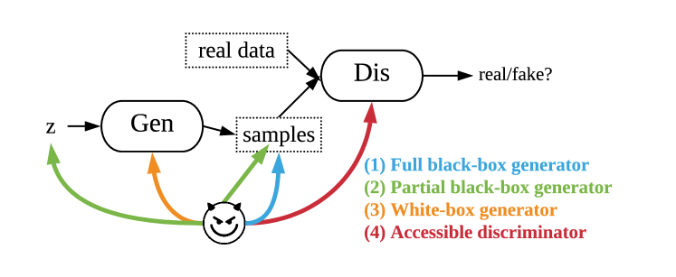
Figure 1. Taxonomy of attack models against GANs. Gen: generator; Dis: discriminator; z: latent code input to Gen.

Taxonomy of Membership Inference Attacks against Deep Generative Models:  We conduct a pioneering study to categorize attack settings against deep generative models. Given the increasing order of the amount of knowledge about a victim model, the settings are benchmarked as (1) full black-box generator, (2) partial black-box generator, (3) white-box generator, and (4) accessible discriminator (full model). In particular, two of the settings, the partial black-box and white-box settings, are of practical value but have not been explored by previous works. We then establish the first taxonomy that comprises the existing and our proposed attacks. See Section 4, Table 1, and Figure 1 for details.

Generic Attack Model and its Novel Instantiated Variants:  We propose a simple and generic attack model (Section 5.1) applicable to all the practical settings and various types of deep generative models. More specifically, our generic attack model can be instantiated to a preliminary low-skill attack for the full black-box setting (Section 5.2), a novel black-box optimization-based attack variant in the partial black-box (Section 5.3), as well as a novel quasi-Newton optimization-based variant in the white-box settings (Section 5.4). The consistent effectiveness of our attack model exhibited in all of the aforementioned settings bridges the assumption gap and performance gap between the full black-box attacks and discriminator-accessible attack in previous study (Hayes et al., 2019; Hilprecht et al., 2019) through a complete performance spectrum (Section 6.7).

Novel Attack Calibration Technique:  To further improve the effectiveness of our attack model, we adjust our approach to each query sample and propose our novel attack calibration technique, which is naturally incorporated in our generic attack framework. Moreover, we prove its near-optimality under a Bayesian perspective. Through extensive experiments, we validate that our attack calibration technique boosts the attack performance noticeably in all cases, across different attack settings, data modalities, and training configurations. See Section 5.6 for detailed explanation and Section 6.6 for experiment results.

Systematic Analysis in Each Setting:  We progressively investigate attacks in each setting in the increasing order of amount of knowledge to adversary. See Section 6.3 to Section 6.5 for detailed elaboration. In each setting, our research spans several orthogonal dimensions including three datasets with diverse modalities (Section 6.1), five victim GAN models that were the state-of-the-art at their release time (Section 6.1), two analysis study w.r.t. GAN training configuration (Section 6.2), attack performance gains introduced by attack calibration (Section 5.6 and Section 6.6) and differential private defense (Section 6.8).

2. Related Work

Generative Models:  Generative models are designed for approximating the probability distribution of the real data. In general, this is done by defining a parametric family of densities and finding the optimal parameters that either maximize the real data likelihood or minimize the divergence between generated and real data distribution. Recent generative models exploit the representation power of deep neural networks for constituting an exceptionally rich parametric family, resulting in tremendous success in modeling high-dimensional data distribution. In this work, we investigate the most widely used deep generative models, namely the generative adversarial networks (GANs) (Goodfellow et al., 2014; Radford et al., 2015; Salimans et al., 2016; Arjovsky et al., 2017; Gulrajani et al., 2017; Karras et al., 2018; Brock et al., 2019; Karras et al., 2019; Karras et al., 2020; Yu et al., 2020) and variational autoencoders (VAEs) (Dinh et al., 2015, 2017; Kingma and Dhariwal, 2018). Briefly speaking, GANs are trained to minimize the divergence between the generated and real data distribution, while VAEs maximize a lower bound of the real data log-likelihood.

Membership Inference Attacks (MIAs):  Shokri et al. (Shokri et al., 2017) specifies the first MIA against discriminative models in the black-box setting, where an attack has access to the victim model’s full response (i.e., confidence scores for all classes) for a given input query. They propose to train shadow models that imitate the behavior of the victim model, which generates data to train an attacker model.

Hayes et al. (Hayes et al., 2019) consider MIA against GANs and also propose to retrain a shadow model of the victim model in the black-box case. They then check the discriminator’s output scores to query inputs and set a threshold such that all the query inputs with scores larger than the threshold will be classified as in the training set.

Another concurrent study by Hilprecht et al. (Hilprecht et al., 2019) investigates MIA against both GANs and VAEs. For VAEs, they assume the accessibility of the full model and propose to threshold the $L_{2}$ reconstruction error; For GANs, they only consider the full black-box setting. Their black-box attack is similar to ours in spirit, as they count the number of generated samples that are inside an $\epsilon$-ball of the query, while we exploit the reconstruction distance instead.

Differential Privacy (DP):  Differential privacy (Dwork and Roth, 2014) is designed to protect the membership privacy of individual samples and is by constructing a defense mechanism against MIA. Recent works propose to train GAN models with differential privacy constraint (Beaulieu-Jones et al., 2019; Acs et al., 2017; Zhang et al., 2018b; Xie et al., 2018; Jordon et al., 2019; Chen et al., 2020) and publicize the DP-trained models instead of the raw data, which allows sharing sensitive data while preserving privacy. The differential privacy constraint is fulfilled by replacing the regular stochastic gradient descent with differential private stochastic gradient descent (DP-SGD) (Abadi et al., 2016), which injects calibrated noise in training gradients. As a result, it perturbs data-related objective functions and mitigates inference attacks.

3. Background

3.1. Generative Model

Generative Adversarial Networks (GANs):  GANs consist of two neural network modules, a generator $G$ and a discriminator $D$, which are trained simultaneously in an adversarial manner. The generator takes random noise $z$ (latent code) as input and generates samples that approximate the training data distribution, while the discriminator receives samples from both the generator and training dataset and is trained to differentiate the two sources. During training, these two modules compete and evolve, such that the generator learns to generate more and more realistic samples aiming at fooling the discriminator, while the discriminator learns to tell the two sources apart more accurately. The training objective can be formulated as

$$\min_{\theta_{G}}\max_{\theta_{D}}\mathbb{E}_{x\sim P_{\text{data}}}[\log(D_{\theta_{D}}(x))]+\mathbb{E}_{z\sim P_{z}}[\log(1-D_{\theta_{D}}(G_{\theta_{G}}(z)))]$$

where $\theta_{G},\theta_{D}$ denote the parameters of the generator and the discriminator. $P_{\text{data}}$ is the real data distribution, while the $P_{z}$ is the prior distribution of the latent code. The first term in the objective forces the discriminator to output high score given real data sample. The second term makes discriminator output low score on generated samples, while the generator is trained to maximize the discriminator output score. Once the training is done, the discriminator is no longer useful and will normally be discarded. The generator will receive new latent code samples $z$ drawn from the known prior distribution (normally Gaussian) and output the synthetic data samples, which will be collected and used for the downstream task.

Variational Autoencoder (VAE):  VAE is another widely used generative framework (Kingma and Welling, 2014; Rezende et al., 2014; Yan et al., 2016) consists of an encoder and a decoder, which are cascaded to reconstruct data with pre-defined similarity metrics, e.g. $L_{1}$/$L_{2}$ loss. The encoder maps data into a latent space, while the decoder maps the encoded latent representation back to the data space. The VAE objective is composed of the reconstruction error and the prior regularization over the latent code distribution. Formally,

$$\min_{\theta,\phi}-\mathbb{E}_{q_{\phi}(z|x)}[p_{\theta}(x|z)]+KL(q_{\phi}(z|x)\|P_{z})$$

where $z$ denotes the latent code, $x$ denotes the input data, $q_{\phi}(z|x)$ is the probabilistic encoder parameterized by $\phi$ which is introduced to approximate the intractable true posterior, $p_{\theta}(x|z)$ represents the probabilistic decoder parameterized by $\theta$, and $KL(\cdot\|\cdot)$ denotes the KL divergence. In practice, $q_{\phi}(z|x)$ is always constrained to be uni-modal Gaussian and $z$ is sampled via the reparameterization trick, which results in a closed-form derivation of the second term.

Hybrid Model:  GANs often suffer from mode collapse and mode dropping issues, i.e., failing to generate appearances relevant to some training samples (low recall), due to the lack of explicit supervison (e.g. data reconstruction) for promoting data mode coverage. VAEs, on the contrary, attain better data coverage but often lack flexible generation capability (low precision). Therefore, a hybrid model, VAEGAN (Larsen et al., 2016; Bhattacharyya et al., 2019), is proposed to jointly train a VAE and a GAN, where the VAE decoder and the GAN generator are collapsed into one by sharing trainable parameters. The GAN discriminator is trained to complement the low-level $L_{1}$ or $L_{2}$ reconstruction loss, in order to improve the generation quality of fine-grained details.

3.2. Membership Inference

We formulate the membership inference attack as a binary classification task where the attacker aims to classify whether a sample $x$ has been used to train a victim generative model. Formally, we define

$$\mathcal{A}:(x,\mathcal{M}(\theta))\rightarrow\{0,1\}$$

where the attack model $\mathcal{A}$ output 1 if the attacker infers that the query sample $x$ is included in the training set, and 0 otherwise. $\theta$ denotes the victim model parameters while $\mathcal{M}$ represents the general model publishing mechanism, i.e., type of access available to the attacker. For example, the $\mathcal{M}$ is an identity function for the white-box access case and can be the inference function for the black-box case. For simplicity, we may omit the dependence on $\mathcal{M}$ if the type of access is irrelevant for illustration. With a Bayesian perspective (Sablayrolles et al., 2019), the optimal attacker aims to compute the probability $P(x\in D_{\text{train}}|x,\theta)$ and predict the query sample to be in the training set if the log-likelihood ratio is non-negative, i.e. the query sample is more likely to be contained in the training set than not. Mathematically,

(1) $$\mathcal{A}(x,\mathcal{M}(\theta))=\mathbbm{1}\left[\log\frac{P(x\in D_{\text{train}}|x,\theta)}{P(x\notin D_{\text{train}}|x,\theta)}\geq 0\right]$$

where $\mathbbm{1}(\cdot)$ is the indicator function, and the training set is denoted by $D_{\text{train}}$. We denote the query sample set as $S=\{(x_{i},m_{i})\}_{i=1}^{N}$ that contains both training set samples ($x_{i}\in D_{\text{train}},m_{i}=1$) as well as hold-out set samples ($x_{i}\notin{D_{\text{train}}},m_{i}=0$), where $m$ is the membership indicator variable. The true positive and true negative rate of the attacker can be measure by $\mathbb{E}_{x_{i}}[P(\mathcal{A}(x_{i},\mathcal{M}(\theta))=1|m_{i}=1)]$ and $\mathbb{E}_{x_{i}}[P(\mathcal{A}(x_{i},\mathcal{M}(\theta))=0|m_{i}=0)]$, respectively.

4. Taxonomy

Latent Gen- Dis- code erator criminator (Hayes et al., 2019) full black-box $\times$ $\blacksquare$ $\times$ (Hilprecht et al., 2019) full black-box $\times$ $\blacksquare$ $\times$ Our full black-box (Section 5.2) $\times$ $\blacksquare$ $\times$ Our partial black-box (Section 5.3) $\checkmark$ $\blacksquare$ $\times$ Our white-box (Section 5.4) $\checkmark$ $\square$ $\times$ (Hayes et al., 2019) accessible discriminator (full model) $\checkmark$ $\square$ $\checkmark$

Table 1. Taxonomy of attack settings against GANs over the previous work and ours. ($\times$: without access; $\checkmark$: with access; $\blacksquare$: black-box; $\square$: white-box).

The attack scenarios can be categorized into either white-box or black-box one. In the white-box setting, the adversary has access to the victim model internals, whereas in the black-box setting, the internal workings are unknown to the attackers. For attacks against GANs, we further distinguish the settings based on the accessibility of GANs’ components, i.e., the latent code, generator model, and the discriminator model, according to the following criteria: (1) whether the discriminator is accessible, (2) whether the generator is accessible, and (3) whether the latent code is accessible. We elaborate on each category in the following in a decreasing order of the amount of knowledge to attackers. Note that we define the taxonomy in a fully attack-agnostic way, i.e. the attacker can freely decide which part of the available information to use.

4.1. Accessible Discriminator (Full Model)

By construction, the discriminator is only used for the adversarial training and normally will be discarded after the training stage is completed. The only scenario in which the discriminator is accessible to the attacker is that the developers publish the whole GAN model along with the source code and allow fine-tuning. In this case, both the discriminator and the generator are accessible to the adversary in a white-box manner. This is the most knowledgeable setting for attackers. And the existing attack methods against discriminative models (Shokri et al., 2017) can be applied to this setting. This setting is also considered in (Hayes et al., 2019), corresponding to the last row in Table 1. In practice, however, the discriminator of a well-trained GAN is discarded without being deployed to APIs, and thus not accessible to attackers. We, therefore, devote less effort to investigating the discriminator and mainly focus on the following practical and generic settings where the attackers only have access to the generator.

4.2. White-box Generator

Following the common practice, researchers from the generative modeling community always publish their well-trained generators and code, which allows users to generate new samples and validate the results. This corresponds to the settings that the generator is accessible to the adversary in a white-box manner, i.e. the attackers have access to the internals of the generator. This scenario is also commonly studied in the community of differential privacy (Dwork et al., 2006) and privacy preserving data generation (Beaulieu-Jones et al., 2019; Acs et al., 2017; Zhang et al., 2018b; Xie et al., 2018; Jordon et al., 2019; Chen et al., 2020), where people enforce privacy guarantee by training and sharing their generative models instead of sharing the raw private data. Our attack model under this setting can serve as a practical tool for empirically estimating the privacy risk incurred by sharing the differentially private generative models, which offers clear interpretability towards bridging between theory and practice. However, this setting has not been explored by any previous work and is a novel case for constructing a membership inference attack against GANs. It corresponds to the second last row in Table 1 and Section 5.4.

4.3. Partial Black-box Generator (Known Input-output Pair)

This is a less knowledgeable setting to attackers where they have no access to the internals of the generator but have access to the latent code of each generated sample. This is a practical setting where the developers retain ownership of their well-trained models while allowing users to control the properties of the generated samples by manipulating the latent code distribution (Jahanian et al., 2019), which is a desired feature for application scenarios such as GAN-based image processing (Gu et al., 2019) and facial attribute editing (Karras et al., 2019; He et al., 2018). This is another novel setting and not considered in previous works (Hayes et al., 2019; Hilprecht et al., 2019). It corresponds to the third last row in Table 1 and Section 5.3.

4.4. Full Black-box Generator (Known Output Only)

This is the least knowledgeable setting to attackers where they are passive, i.e., unable to provide input, but are only permitted to access the generated samples set from the well-trained black-box generator. Hayes et al. (Hayes et al., 2019) investigate attacks in this setting by retraining a local copy of the victim model. Hilprecht et al. (Hilprecht et al., 2019) count the number of generated samples that are inside an $\epsilon$-ball of the query, based on an elaborate design of distance metric. Our idea is similar in spirit to Hilprecht et al. (Hilprecht et al., 2019) but we score each query by the reconstruction error directly, which does not introduce additional hyperparameter while achieving superior performance. In short, we design a low-skill attack method with a simpler implementation (Section 5.2) that achieves comparable or better performance (Section 6.3). Our attack and theirs correspond to the third, second, and first rows in Table 1, respectively.

5. Attack Model

Notation Description $\mathcal{A}$ Attacker $\mathcal{M}$ model publishing mechanism $D_{\text{train}}$ Training set of the victim generator $S$ Query set $\mathcal{R}$ Attacker’s reconstructor $x$ Query sample $m$ Membership indicator variable $z$ Latent code (input to the generator) $\mathcal{G}_{v}$ Victim generator $\mathcal{G}_{r}$ Attacker’s reference generator, described in Section 5.6 $\theta_{v}$ Victim model’s parameter $\theta_{r}$ Attacker’s reference model’s parameter

Table 2. Notations.

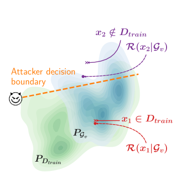
(a) Generic attack model (Section 5.1)

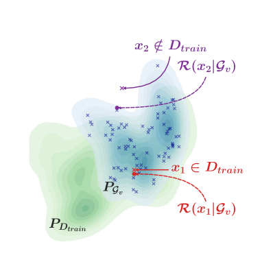
(b) Full black-box attack (Section 5.2)

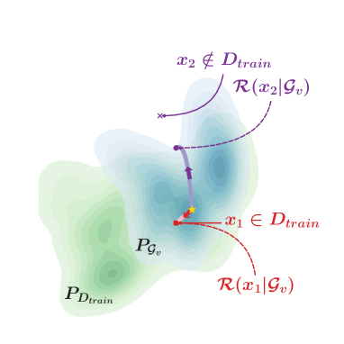
(c) Partial black-box and white-box attack (Section 5.3 and Section 5.4)

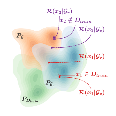
(d) Attack calibration (Section 5.6)

Figure 2. Diagram of our attacks. Mathematical notations refer to Table 2. $P$ represents data distribution. $x_{1}$ belongs to $D_{\text{train}}$ so that it should be better represented by $\mathcal{G}_{v}$ with a smaller distance to its reconstructed copy $\mathcal{R}(x_{1}|\mathcal{G}_{v})$. $x_{2}$ does not belong to $D_{\text{train}}$ so that it should have a larger distance to its best approximation $\mathcal{R}(x_{2}|\mathcal{G}_{v})$ in $P_{\mathcal{G}_{v}}$. (a) Our generic attacker set a decision boundary based on the reconstruction distance to infer membership. (b) The best reconstruction is determined over random samples from $P_{\mathcal{G}_{v}}$ while in (c) it is found by optimization on the manifold of $P_{\mathcal{G}_{v}}$. (d) $P_{\mathcal{G}_{r}}$ is a third-party reference GAN distribution where the reconstruction distance is calibrated by the distance between $x$ and $\mathcal{R}(x|\mathcal{G}_{r})$.

5.1. Generic Attack Model

As mentioned in Section 3.2, the optimal attacker computes the probability $P(m_{i}=1|x_{i},\theta_{v})$. Specifically for the generative model, we make the assumption that this probability should be proportional to the probability that the query sample can be generated by the generator. This assumption holds in general as the generative model is trained to approximate the training data distribution, i.e., $P_{\mathcal{G}_{v}}\approx P_{D_{\text{train}}}$ where $\mathcal{G}_{v}$ denotes the victim generator. And if the probability that the query sample is generated by the victim generator is large, it is more likely that the query sample is used to train the generative model. Formally,

(2) $$P(m_{i}=1|x_{i},\theta_{v})\propto P_{\mathcal{G}_{v}}(x|\theta_{v})$$

However, computing the exact probability is intractable as the distribution of the generated data cannot be represented with an explicit density function. Therefore, we adopt the Parzen window density estimation (Duda et al., 2012) and approximate the probability as below,

(3) $$P_{\mathcal{G}_{v}}(x|\theta_{v}) =\frac{1}{k}\sum_{i=1}^{k}\phi(x,\mathcal{G}_{v}(z_{i}));\quad z_{i}\sim P_{z}$$

(4) $$\approx\frac{1}{k}\sum_{i=1}^{k}\exp(-L(x,\mathcal{G}_{v}(z_{i})));\quad z_{i}\sim P_{z}$$

where $\phi(\cdot,\cdot)$ denotes the kernel function, $L(\cdot,\cdot)$ is the general distance metric defined in Section 5.5, and $k$ is the number of samples. Note that this can be further simplified and well approximated using only few samples (Boiman et al., 2008), as all of the terms in the summation of Equation 3, except for a few, will be negligible since $\phi(x,y)$ exponentially decreases with distance between $x,y$.

5.2. Full Black-box Attack

We start with the least knowledgeable setting where an attacker only has access to a black-box generator $\mathcal{G}_{v}$. The attacker is allowed no other operation but blindly collecting $k$ samples from $\mathcal{G}_{v}$, denoted as $\{\mathcal{G}_{v}(\cdot)_{i}\}_{i=1}^{k}$. $\mathcal{G}_{v}(\cdot)$ indicates that the attacker has neither access nor control over latent code input. We then approximate the probability in Equation 4 using the largest term which is given by the nearest neighbor to $x$ among $\{\mathcal{G}_{v}(\cdot)_{i}\}_{i=1}^{k}$. Formally,

(5) $$\mathcal{R}(x|\mathcal{G}_{v})=\operatorname*{argmin}_{\hat{x}\in\{\mathcal{G}_{v}(\cdot)_{i}\}_{i=1}^{k}}L(x,\hat{x})$$

See Figure 2(b) for a diagram. This approximation bound the complete Parzen window from below, but in practice we observe almost no difference when incorporating more terms in the summation for a fixed $k$. However, we find the estimation more sensitive to $k$, and in general a larger $k$ leads to better reconstructions (Figure 10) but at the price of a higher query and computation cost. Throughout the experiments, we consider a practical and limited budget and choose $k$ to be of the same magnitude as the training dataset size.

5.3. Partial Black-box Attack

In some practical scenario discussed in Section 4.3, the access to the latent code $z$ is permitted. We then propose to exploit $z$ in order to find a better reconstruction of the query sample and thus improve the $P_{\mathcal{G}_{v}}(x|\theta_{v})$ estimation. Concretely, the attacker performs an black-box optimization with respect to $z$. Formally,

(6) $$\mathcal{R}(x|\mathcal{G}_{v})=\mathcal{G}_{v}(z^{*})$$

where

(7) $$z^{*}=\operatorname*{argmin}_{z}L\big{(}x,\mathcal{G}_{v}(z)\big{)}$$

Without knowing the internals of $\mathcal{G}_{v}$, the optimization is not differentiable and no gradient information is available. As only the evaluation of function (forward-pass through the generator) is allowed by the access of $\{z,\mathcal{G}_{v}(z)\}$ pair, we propose to approximate the optimum via the Powell’s Conjugate Direction Method (Powell, 1964).

5.4. White-box Attack

In the white-box setting, we have the same reconstruction formulation as in Section 5.3. See Figure 2(c) for a diagram. More advantageously to attackers, the reconstruction quality can be further boosted thanks to access to the internals of $\mathcal{G}_{v}$. With access to the gradient information, the optimization problem can be more accurately solved by advanced first-order optimization algorithms (Kingma and Ba, 2015; Tieleman and Hinton, 2012; Liu and Nocedal, 1989). In our experiment, we apply the L-BFGS algorithm for its robustness against suboptimal initialization and its superior convergence rate in comparison to the other methods.

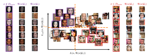
Figure 3. The effectiveness of calibration when attacking PGGAN on CelebA. The x- and y-axes respectively represent the distance before ($L$) and after calibration ($L_{\text{cal}}$) between a query sample $x$ and its reconstruction $\mathcal{R}(x|\mathcal{G}_{v})$. $\epsilon$ and $\epsilon_{\text{cal}}$ are the corresponding thresholds for classification. The false-positive (in purple frame) as well as the false-negative samples (in red frame) before ($L$) calibration can be corrected by calibration ($L_{\text{cal}}$).

5.5. Distance Metric

Our distance metric $L(\cdot,\cdot)$ consists of three terms: the element-wise (pixel-wise) difference term $L_{2}$ targets low-frequency components, the deep image feature term $L_{\text{lpips}}$ (i.e., the Learned Perceptual Image Patch Similarity (LPIPS) metric (Zhang et al., 2018a)) targets realism details, and the regularization term penalizes latent code far from the prior distribution. Mathematically,

$$L\big{(}x,\mathcal{G}_{v}(z)\big{)}= \lambda_{1}L_{2}\big{(}x,\mathcal{G}_{v}(z)\big{)}+\lambda_{2}L_{\text{lpips}}\big{(}x,\mathcal{G}_{v}(z)\big{)}$$

(8) $$+\lambda_{3}L_{\text{reg}}(z)$$

where

(9) $$L_{2}\big{(}x,\mathcal{G}_{v}(z)\big{)}=\|x-\mathcal{G}_{v}(z)\|_{2}^{2}$$

(10) $$L_{\text{reg}}(z)=\big{(}\|z\|_{2}^{2}-\text{dim}(z)\big{)}^{2}$$

$\lambda_{1}$, $\lambda_{2}$ and $\lambda_{3}$ are used to enable/disable and balance the order of magnitude of each loss term. For non-image data, $\lambda_{2}=0$ because LPIPS is no longer applicable. For full black-box attack, $\lambda_{3}=0$ as the constraint $z\sim P_{z}$ is satisfied by the sampling process.

5.6. Attack Calibration

We noticed that the reconstruction error is query-dependent, i.e., some query samples are more (less) difficult to reconstruct due to their intrinsically more (less) complicated representations, regardless of which generator is used. In this case, the reconstruction error is dominated by the representations rather than by the membership clues. We, therefore, propose to mitigate the query dependency by first independently training a reference GAN $\mathcal{G}_{r}$ with a relevant but disjoint dataset, and then calibrating our base reconstruction error according to the reference reconstruction error. Formally,

(11) $$L_{\text{cal}}\big{(}x,\mathcal{R}(x|\mathcal{G}_{v})\big{)}=L\big{(}x,\mathcal{R}(x|\mathcal{G}_{v})\big{)}-L\big{(}x,\mathcal{R}(x|\mathcal{G}_{r})\big{)}$$

with $\mathcal{R}$ the reconstruction. As demonstrated in Figure 3, we show in the up-left quadrant the query samples in purple frame that are classified as in $D_{\text{train}}$ by $L$ and as not in $D_{\text{train}}$ by $L_{\text{cal}}$. They are false-positive to $L$ but are corrected to true-negative by $L_{\text{cal}}$. On the other hand, we show in the bottom-right quadrant the query samples in red frame that are classified as not in $D_{\text{train}}$ by $L$ and as in $D_{\text{train}}$ by $L_{\text{cal}}$. They are false-negative to $L$ but are corrected to true-positive by $L_{\text{cal}}$. We compare all these samples, their reconstructions from the victim generator $\mathcal{G}_{v}$, and their reconstructions from the reference generator $\mathcal{G}_{r}$ on the two sides of the plot. The false-positive samples by $L$ on the left-hand side are those with less complicated appearances such that their reconstruction errors are not high given arbitrary generators. In contrast, the false-negative samples by $L$ on the right-hand side are those with more complicated appearances such that their reconstruction errors are high given arbitrary generators. Our calibration can effectively mitigate these two types of misclassification that depend on sample representations.

As discussed in Section 3.2, the optimal attacker aims to compute the membership probability

(12) $$P(m_{i}=1|\theta_{v},x_{i})=\mathbb{E}_{S}[P(m_{i}=1|\theta_{v},x_{i},S)]$$

Specifically, inferring the membership of the query sample $x_{i}$ amounts to approximating the value of $P(m_{i}=1|\theta_{v},x_{i},S)$ (Sablayrolles et al., 2019). We show that our calibrated loss well approximate this probability by the following theorem, whose proof is provided in Appendix.

Theorem 5.1.

Given the victim model with parameter $\theta_{v}$, a query dataset $S$, the membership probability of a query sample $x_{i}$ is well approximated by the sigmoid of minus calibrated reconstruction error.

(13) $$P(m_{i}=1|\theta_{v},x_{i},S)\approx\sigma(-L_{\text{cal}}(x_{i},\mathcal{R}(x_{i}|\mathcal{G}_{v}))$$

And the optimal attack is equivalent to

(14) $$\mathcal{A}(x_{i},\mathcal{M}(\theta_{v}))=\mathbbm{1}[L_{\text{cal}}(x_{i},\mathcal{R}(x_{i}|\mathcal{G}_{v}))<\epsilon]$$

i.e., the attacker checks whether the calibrated reconstruction error of the query sample $x_{i}$ is smaller than a threshold $\epsilon$.

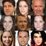
(a) PGGAN

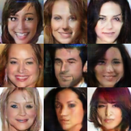
(b) WGANGP

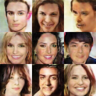
(c) DCGAN

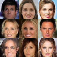
(d) VAEGAN

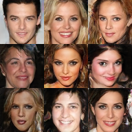
(e) PGGAN w/ DP

Figure 4. Generated images from different victim GAN models trained on CelebA.

In the white-box case, the reference model has the same architecture as the victim model as this information is accessible to the attacker. In the full black-box and partial black-box settings, $\mathcal{G}_{r}$ has irrelevant network architectures to $\mathcal{G}_{v}$, which is fixed across attack scenarios. The optimization on the well-trained $\mathcal{G}_{r}$ is the same as on the white-box $\mathcal{G}_{v}$. See Figure 2(d) for a diagram, and Section 6.6 for implementation details.

6. Experiments

Based on the proposed taxonomy, we present the most comprehensive evaluation to date on the membership inference attacks against deep generative models. While prior studies have singled out few data sets from constraint domains on selected models, our evaluation includes three diverse datasets, five different generative models, and systematic analysis of attack vectors – including more viable threat models. Via this approach, we present key discoveries, that connect for the first time the effectiveness of the attacks to the model types, data sets, and training configuration.

6.1. Setup

Datasets:  We conduct experiments on three diverse modalities of datasets covering images, medical records, and location check-ins, which are considered with a high risk of privacy breach.

CelebA (Liu et al., 2015) is a large-scale face attributes dataset with 200k RGB images. Images are aligned to each other based on facial landmarks, which benefits GAN performance. We select at most 20k images, center-crop them, and resize them to $64\times 64$ before GAN training.

MIMIC-III (Johnson et al., 2016) is a public Electronic Health Records (EHR) database containing medical records of $46,520$ intensive care unit (ICU) patients. We follow the same procedure as in (Choi et al., 2018) to pre-process the data, where each patient is represented by a 1071-dimensional binary feature vector. We filter out patients with repeated vector presentations and yield $41,307$ unique samples.

Instagram New-York (Backes et al., 2017) contains Instagram users’ check-ins at various locations in New York at different time stamps from 2013 to 2017. We filter out users with less than 100 check-ins and yield $34,336$ remaining samples. For sample representation, we first select $2,024$ evenly-distributed time stamps. We then concatenate the longitude and latitude values of the check-in location at each time stamp, and yield a 4048-dimensional vector for each sample. The longitude and latitude values are either retrieved from the dataset or linearly interpolated from the available neighboring time stamps. We then perform zero-mean normalization before GAN training.

Victim GAN Models:  We select PGGAN (Karras et al., 2018), WGANGP (Gulrajani et al., 2017), DCGAN (Radford et al., 2015), MEDGAN (Choi et al., 2018), and VAEGAN (Bhattacharyya et al., 2019) into the victim model set, considering their pleasing performance on generating images and/or other data representations.

It is important to guarantee the high quality of well-trained GANs because attackers are more likely to target high-quality GANs with practical effectiveness. We noticed previous works (Hayes et al., 2019; Hilprecht et al., 2019) only show qualitative results of their victim GANs. In particular, Hayes et al. (Hayes et al., 2019) did not show visually pleasing generated results on the Labeled Faces in the Wild (LFW) dataset (Huang et al., 2008). Rather, we present better qualitative results of different GANs on CelebA (Figure 4), and further present the corresponding quantitative evaluation in terms of Fréchet Inception Distance (FID) metric (Heusel et al., 2017) (Table 3). A smaller FID indicates the generated image set is more realistic and closer to real-world data distribution. We show that our GAN models are in a reasonable range to the state of the art.

PG- WGAN- DC- VAE- SOTA PGGAN GAN GP GAN GAN ref w/ DP FID 14.86 24.26 35.40 53.08 7.40 15.63

Table 3. FID for different GAN models trained on CelebA. “SOTA ref” represents the state-of-the-art result reported in (Brock et al., 2019) over $128\times 128$ ImageNet ILSVRC 2012 dataset (Russakovsky et al., 2015). “w/ DP” represents the GAN model with DP privacy protection (Abadi et al., 2016) (see Section 6.8).

Attack Evaluation:  The proposed membership inference attack is formulated as a binary classification given a threshold $\epsilon$ in Equation 14. Through varying $\epsilon$, we measure the area under the receiver operating characteristic curve (AUCROC) to evaluate the attack performance.

6.2. Analysis Study

We first list two dimensions of analysis study across attack settings. There are also some other dimensions specifically for the white-box attack, which are elaborated in Section 6.5.

6.2.1. GAN Training Set Size

Training set size is highly related to the degree of overfitting of GAN training. A GAN model trained with a smaller size tends to more easily memorize individual training images and is thus more vulnerable to membership inference attack. Moreover, training set size is the main factor that affects the privacy cost computation for differential privacy. Therefore, we evaluate the attack performance w.r.t. training set size. We exclude DCGAN and VAEGAN from evaluation since they yield unstable training for small training sets.

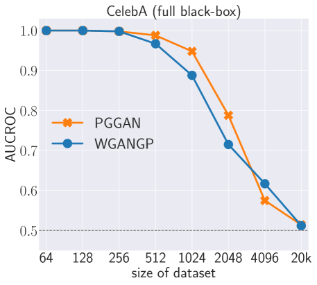
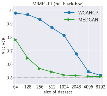
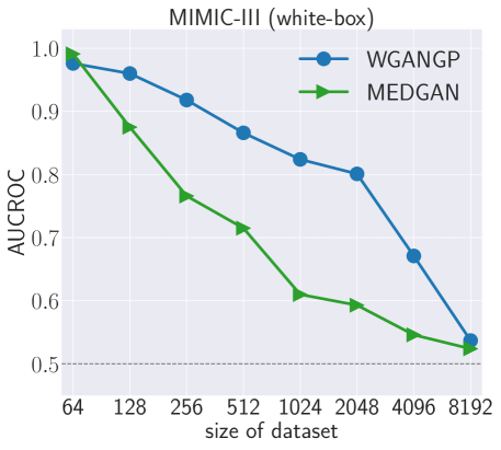
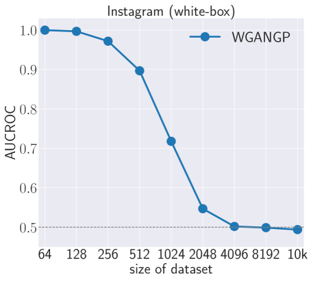
Figure 5. Full black-box attack (the first row) and white-box attack (the second row) performance w.r.t. GAN training set size.

6.2.2. Random v.s. Identity-based Selection for GAN Training Set

There are different levels of difficulty for membership inference attack. For example, CelebA contains person identity information and we can design attack difficulty by composing GAN training set based on identity or not. In one case, we include all images of the selected individuals for training(identity). In the other case, we ignore identity information and randomly select images for training(random), i.e., it is possible that some images for an individual are in the training dataset while some are not. The former case is relatively easier to attackers with a larger margin between membership image set and non-membership image set. In line with previous work (Hayes et al., 2019), we evaluate these two kinds of training set selection schemes on CelebA for a complete and fair comparison.

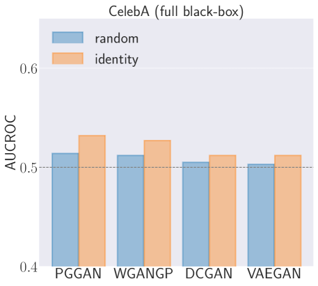
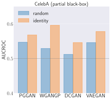
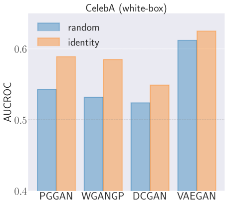
Figure 6. Attack performance on the random v.s. identity-based training set selection (CelebA with size=20k).

6.3. Evaluation on Full Black-box Attack

We start with evaluating our preliminary low-skill black-box attack model in order to gain a sense of the difficulty of the whole problem.

6.3.1. Performance w.r.t. GAN Training Set Size

Figure 5 to Figure 5 plot the attack performance against different GAN models on the three datasets. As shown in the plots, the attack performs sufficiently well when the training set is small for all three datasets. For instance, on CelebA, when the training set contains up to 512 images, attacker’s AUCROC on both PGGAN and WGANGP are above 0.95. This indicates an almost perfect attack and a serious privacy breach. For larger training sets, however, the attacks become less effective as the degree of overfitting decreases and GAN’s capability shifts from memorization to generalization. It is also consistent with the objective of GAN, i.e., to model the underlying distribution of the whole population instead of fitting a particular data sample. Hence, the collection of more data for GAN training can reduce privacy breach of individual samples. Moreover, PGGAN becomes more vulnerable than WGANGP on CelebA when the training size becomes larger. WGANGP is consistently more vulnerable than MEDGAN on MIMIC-III regardless of training size.

6.3.2. Performance w.r.t. GAN Training Set Selection

Figure 6 shows the attack performance w.r.t. training set selection schemes on four victim GAN models when fixing the training set size. We observe that, consistently, all the GAN models are more vulnerable when the training set is selected based on identity. Hence, more attention needs to be paid to an identity-based privacy breach, which is more likely to happen than an instance-based privacy breach. Moreover, when compared among different victim GAN models, DCGAN and VAEGAN are more resistant against the full black-box attack with AUCROC only marginally above 0.5 (random guess baseline). This may be attributed to the poor generation quality of DCGAN and VAEGAN (Table 3), as it indicates that a certain amount of data samples can not be well represented by the victim model and thus the reconstruction error will be a less accurate approximation of the true membership probability in Equation 2.

6.4. Evaluation on Partial Black-box Attack

6.4.1. Performance w.r.t. GAN Training Set Selection

Figure 6 shows the comparison on four victim GAN models. Similar to the case of the full black-box attack (Section 6.3), we find that all models become more vulnerable to identity-based selection. Still, DCGAN is the most resistant victim against membership inference in both training set selection schemes, probably due to its inferior generation quality.

6.4.2. Comparison to Full Black-box Attack

Comparing between Figure 6 and Figure 6, the attack performance against each GAN model consistently and significantly improves from black-box setting to partial black-box setting. We attribute this improvement to a better reconstruction of query samples found by the attacker via optimization. Hence, we conclude that providing the input interface to a generator suffers from an increased privacy risk.

6.5. Evaluation on White-box Attack

We further investigate the case where the victim generator is published in a white-box manner. This scenario is commonly studied in the field of privacy preserving data generation (Beaulieu-Jones et al., 2019; Acs et al., 2017; Zhang et al., 2018b; Xie et al., 2018; Jordon et al., 2019; Chen et al., 2020), where our approach can serve as a simple and interpretable framework for empirically quantifying the privacy leakage. As the optimization in the white-box attack involves more technical details, we conduct additional analysis study and sanity check in this setting. See Appendix C.1 for more details.

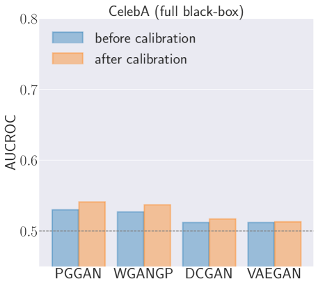
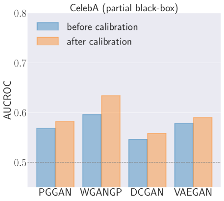
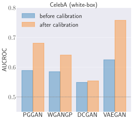
Figure 7. Attack performance before and after calibration on CelebA (size=20k).

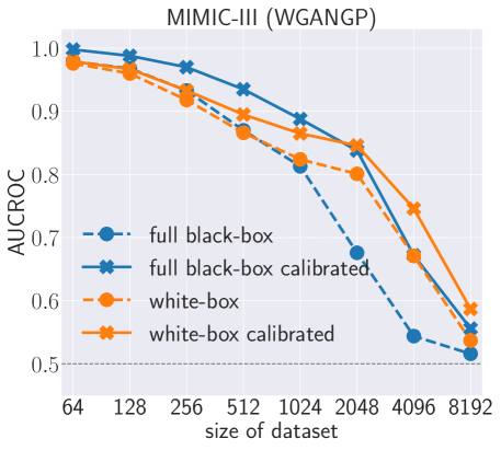
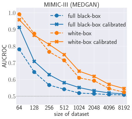
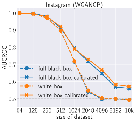
Figure 8. Attack performance before and after calibration for non-image datasets w.r.t. GAN training set sizes.

6.5.1. Performance w.r.t. GAN Training Set Size

Figure 5 to Figure 5 plot the attack performance against different GAN models on the three datasets when varying training set size. We find that the attack becomes less effective as the training set becomes larger, similar to that in the black-box setting. For CelebA, the attack remains effective for 20k training samples, while for MIMIC-III and Instagram, this number decreases to 8192 and 2048, respectively. The strong similarity between the member and non-member in these two non-image datasets increases the difficulty of attack, which explains the deteriorated effectiveness of the attack model.

6.5.2. Performance w.r.t. GAN Training Set Selection

Figure 6 shows the comparisons against four victim GAN models. Our attack is much more effective when composing GAN training set according to identity, which is similar to those in the full and partial black-box settings.

6.5.3. Comparison to Full and Partial Black-box Attacks

For membership inference attack, it is an important question whether or to what extent the white-box attack is more effective than the black-box ones. For discriminative (classification) models, recent literature reports that the state-of-the-art black-box attack performs almost as well as the white-box attack (Sablayrolles et al., 2019; Nasr et al., 2019). In contrast, we find that against generative models the white-box attack is much more effective. Comparisons across subfigures in Figure 6 show that the AUCROC values increase by at least 0.03 when changing from full black-box to white-box setting. Compared to the partial black-box attack, the white-box attack achieves noticeably better performance against PGGAN and VAEGAN. Moreover, conducting the white-box attack requires much less computation cost than conducting the partial black-box attack. Therefore, we conclude that publicizing model parameters (white-box setting) does incur high privacy breach risk.

6.6. Performance Gain from Attack Calibration

We perform calibration on all the settings. Note that for full and partial black-box settings, attackers do not have prior knowledge of victim model architectures. We thus train a PGGAN on LFW face dataset (Huang et al., 2008) and use it as the generic reference model for calibrating all victim models trained on CelebA in the black-box settings. Similarly, for MIMIC-III, we use WGANGP as the reference model for MedGAN and vice versa. In other words, we have to guarantee that our calibrated attacks strictly follow the black-box assumption.

Figure 7 compares attack performance on CelebA before and after applying calibration. The AUCROC values are improved consistently across all the GAN architectures in all the settings. In general, the white-box attack calibration yields the greatest performance gain. Moreover, the improvement is especially significant when attacking against VAEGAN, as the AUCROC value increases by 0.2 after applying calibration.

Figure 8 compares attack performance on the other two non-image datasets. The performance is also consistently boosted for all training set sizes after calibration.

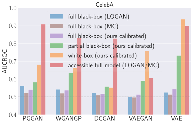
Figure 9. Comparison of different attacks on CelebA. See Table 12 in Appendix for quantitative results.

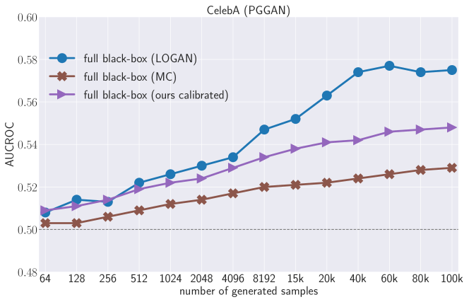
Figure 10. Full black-box attack performance against PGGAN on CelebA w.r.t. $k$ in Equation 5, the number of generated samples. See Table 14 in Appendix for quantitative results.

6.7. Comparison to Baseline Attacks

We compare our calibrated attack to two recent membership inference attack baselines: Hayes et al. (Hayes et al., 2019) (denoted as LOGAN) and Hilprecht et al. (Hilprecht et al., 2019) (denoted as MC, standing for their proposed Monte Carlo sampling method). As described in our taxonomy (Section 4), LOGAN includes a full black-box attack model and a discriminator-accessible attack model against GANs. The latter is regarded as the most knowledgeable but unrealistic setting because the discriminator in GAN is usually not accessible in practice. But we still compare to both settings for the completeness of our taxonomy and experiments. MC includes a full black-box attack against GANs and a full-model-accessible attack against VAEs. We evaluate our generic attack model on both GANs and VAEs for a complete comparison, though we mainly focus on GANs in this work. Note that, to the best of our knowledge, there does not exist any attack against GANs in the partial black-box or white-box settings.

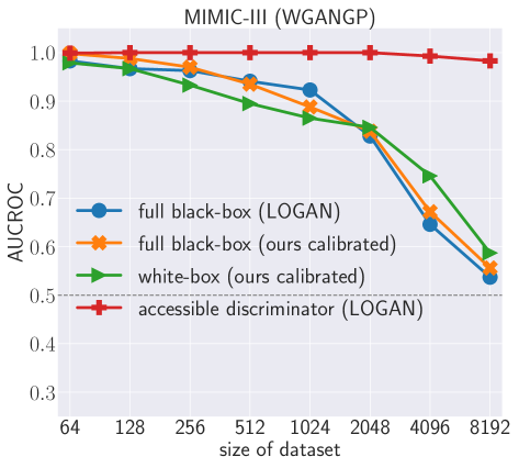
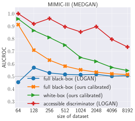
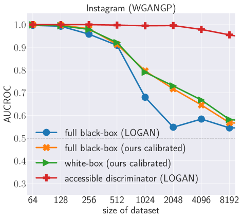
Figure 11. Comparison of different attacks on the other two non-image datasets w.r.t. GAN training set size. See Table 13 in Appendix for quantitative results.

Figure 9, Figure 10, and Figure 11 show the comparisons, considering several datasets, victim models, training set sizes, numbers of query images (full black-box), and different attack settings. We skip MC on the non-image datasets as it is not directly applicable in terms of their distance calculation. Our findings are as follows.

In the black-box setting, our low-skill attack consistently outperforms MC and outperforms LOGAN on the non-image datasets. It also achieves comparable performance to LOGAN on CelebA but with a much simpler and learning-free implementation.

Our white-box and even partial black-box attacks consistently outperform the other full black-box attacks. Hence, publicizing the generator or even just the input to the generator can lead to a considerably higher risk of privacy breach. With a complete spectrum of performance across settings, they bridge the performance gap between the highly constrained full black-box attack and the unrealistic discriminator-accessible attack. Moreover, our proposed white-box attack model is of practical value for the differential privacy community.

Assuming the accessibility of discriminator (full model) normally results in the most effective attack. This can be explained by the fact that the discriminator is explicitly trained to maximize the margin between training set (membership samples) and generated set (a subset of non-membership samples), which eventually yields very accurate confidence scores for membership inference. Surprisingly, our calibrated white-box attack even outperforms baseline methods in more knowledgeable settings, i.e., LOGAN (accessible discriminator) for VAEGAN and MC (accessible full model) for VAE. This shows that when data coverage is explicitly enforced, which probably leads to overfitting and data memorization if not properly regularized, our attack models are highly effectively and achieve superior performance with a more realistic assumption.

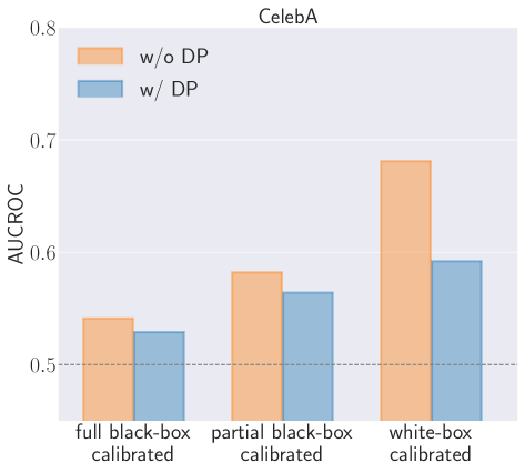
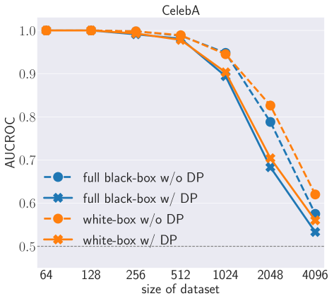
Figure 12. (a) Attack performance against PGGAN on CelebA with or without DP defense. (b)Attack performance against PGGAN on CelebA with or without DP defense, w.r.t. GAN training set size. We fix all the other control factors (training iterations, batch size, noise scale, norm threshold) apart from training set size, which results in less privacy guarantee for a smaller dataset.

6.8. Defense

We investigate the most effective defense mechanism against MIA to date that is applicable to GANs (Hayes et al., 2019; Beaulieu-Jones et al., 2019; Zhang et al., 2018b; Xie et al., 2018), i.e., the differential private (DP) stochastic gradient descent (Abadi et al., 2016). The algorithm can be summarized into two steps. First, the per-sample gradient computed at each training iteration is clipped by its $L_{2}$ norm with a pre-defined threshold. Subsequently, calibrated random noise is added to the gradient in order to inject stochasticity for protecting privacy. In this scheme, however, privacy protection is at the cost of computational complexity and utility deterioration, i.e., slower training and lower generation quality.

We conduct attacks against PGGAN on CelebA, which has been defended by DP. We skip the other cases because DP always deteriorates generation quality to an unacceptable level. The hyper-parameters are selected through the grid search. We fix the norm threshold to 1.0 (average gradient norm magnitude during pre-training) and the noise scale to $10^{-4}$ (the largest value with which we obtain samples of good visual quality). However, this results in high $\epsilon$ values ($>10^{10}$ for a default value of $\delta=10^{-5}$), while it still reduces the effectiveness of the membership inference attack.

Figure 12 and Figure 12 depict the attack performance in different settings. We observe a consistent decrease in AUCROC in all the settings. Therefore, DP is effective in general against our attack. However, applying DP into training leads to a much higher computation cost ($10\times$ slower) in practice due to the per-sample gradient modification. Moreover, DP results in a deterioration of GAN utility, which is witnessed by an increasing FID (comparing the last and second columns in Table 3). Moreover, for obtaining a pleasing level of utility, the noise scale has to be limited to a small value, which, in turn, cannot defend the membership inference attack completely. For example, for all the settings, our attack still achieves better performance than the random guess baseline (AUCROC $=0.5$).

6.9. Summary

Before ending this section, we show a few insights over the experiment results and list practical considerations relevant to the deployment of GANs and potential privacy breaches.

• The vulnerability of models under MIA heavily relies on the attackers’ knowledge about victim models. Releasing the discriminator (full model) results in an exceptionally high risk of privacy breach, which can be explained by the fact that the discriminator had full access to the training data and thus easily memorizes the private information about the training data. Similarly, the release of the generator and/or the control over the input noise $z$ also incurs a relatively high privacy risk.

• The vulnerability of different generative models under MIA varies. Although the effectiveness of MIA mainly depends on the generation quality of victim models, the objective function and training paradigm also play important roles. Specifically, when data reconstruction is explicitly formulated in the training objective to improve data mode coverage, e.g. in VAEGAN and VAE, the resulting models become highly vulnerable to MIA.

• A smaller training dataset leads to a higher risk of revealing information of individual samples. In particular, if the magnitude of training set size is less than $10k$ where most existing GAN models have sufficient modeling capacity for overfitting to individual sample, the membership privacy is highly likely to be compromised once the GAN model and/or its generated sample set is released. This causes special concern when dealing with real-world privacy sensitive datasets (e.g. medical records), which typically contain very limited data samples.

• Differential private defense on GAN training is effective against practical MIA, but at the cost of high computation burden and deteriorated generation quality.

7. Conclusion

We have established the first taxonomy of membership inference attacks against GANs, with which we hope to benchmark research in this direction in the future. We have also proposed the first generic attack model based on reconstruction, which is applicable to all the settings according to the amount of the attacker’s knowledge about the victim model. In particular, the instantiated attack variants in the partial black-box and white-box settings are another novelty that bridges the assumption gap and performance gap in the previous work (Hayes et al., 2019; Hilprecht et al., 2019). In addition, we proposed a novel theoretically grounded attack calibration technique, which consistently improve the attack performance in all cases. Comprehensive experiments show consistent effectiveness and a broad spectrum of performance in a variety of setups spanning diverse dataset modalities, various victim models, two directions of analysis study, attack calibration, as well as differential privacy defense, which conclusively provide a better understanding of privacy risks associated with deep generative models.

Appendix A Proof

Theorem 5.1.

Given the victim model with parameter $\theta_{v}$, a query dataset $S$, the membership probability of a query sample $x_{i}$ is well approximated by the sigmoid of minus calibrated reconstruction error.

(15) $$P(m_{i}=1|\theta_{v},x_{i},S)\approx\sigma(-L_{\text{cal}}(x_{i},\mathcal{R}(x_{i}|\mathcal{G}_{v}))$$

And the optimal attack is equivalent to

(16) $$\mathcal{A}(x_{i},\mathcal{M}(\theta_{v}))=\mathbbm{1}[L_{\text{cal}}(x_{i},\mathcal{R}(x_{i}|\mathcal{G}_{v}))<\epsilon]$$

i.e., the attacker checks whether the calibrated reconstruction error of the query sample $x_{i}$ is smaller than a threshold $\epsilon$.

Proof.

By applying the Bayes rule and the property of sigmoid function $\sigma$, the membership probability can be rewritten as follows (Sablayrolles et al., 2019):

(17) $$P(m_{i}=1|\theta_{v},x_{i},S) =\sigma\left(\log\left(\frac{P(\theta_{v}|m_{i}=1,x_{i},S_{-i})P(m_{i}=1)}{P(\theta_{v}|m_{i}=0,x_{i},S_{-i})P(m_{i}=0)}\right)\right)$$

where $S_{-i}=S\backslash(x_{i},m_{i})$, i.e., the whole query set except the query sample $x_{i}$.

Assuming independence of samples in $\mathcal{S}$ while applying Bayes rule and Product rule, we obtain the following posterior approximation

(18) $$P(\theta_{v}|S) \propto\prod_{\{j|m_{j}=1\}}P(x_{j}|\theta_{v})P(\theta_{v})$$

(19) $$\propto\exp(-\sum_{j}m_{j}\cdot l(x_{j},\theta_{v}))$$

with $l(x_{j},\theta_{v})=L(x_{j},\mathcal{R}(x|\mathcal{G}_{v}))$for brevity. The Equation 18 means that the probability of a certain model parameter is determined by its i.i.d. training set samples. Subsequently, by assuming a uniform prior of the model parameter over the whole parameter space and plug in the results from Equation 4 we obtain Equation 19.

By normalizing the posterior in Equation 19, we obtain

(20) $$P(\theta_{v}|m_{i}=1,x_{i},S_{-i}) =\frac{\exp(-\sum_{j}m_{j}\cdot l(x_{j},\theta_{v}))}{\int_{\theta^{\prime}}\exp(-\sum_{j}m_{j}\cdot l(x_{j},\theta^{\prime}))d_{\theta^{\prime}}}$$

(21) $$P(\theta_{v}|m_{i}=0,x_{i},S_{-i}) =\frac{\exp(-\sum_{j\neq i}m_{j}\cdot l(x_{j},\theta_{v}))}{\int_{\theta^{\prime}}\exp(-\sum_{j\neq i}m_{j}\cdot l(x_{j},\theta^{\prime}))d_{\theta^{\prime}}}$$

with the following ratio:

(22) $$\frac{P(\theta_{v}|m_{i}=1,x_{i},S)}{P(\theta_{v}|m_{i}=0,x_{i},S)} =\frac{\exp(-l(x_{i},\theta_{v}))}{\int_{\theta^{\prime}}\exp(-l(x_{i},\theta^{\prime}))P(\theta^{\prime}|S_{-i})d_{\theta^{\prime}}}$$

where

$$P(\theta|S_{-i})=\frac{\exp(-\sum_{j\neq i}m_{j}\cdot l(x_{j},\theta))}{\int_{\theta^{\prime}}\exp(-\sum_{j\neq i}m_{j}\cdot l(x_{j},\theta^{\prime}))d_{\theta^{\prime}}}$$

Putting things together, we have

$$P(m_{i}=1|\theta_{v},x_{i},S)=\sigma[ \log(\frac{P(m_{i}=1)}{P(m_{i}=0)})-l(x_{i},\theta_{v})$$

(23) $$-\log\left(\int_{\theta^{\prime}}\exp(-l(x_{i},\theta^{\prime}))P(\theta^{\prime}|S_{-i})d_{\theta^{\prime}}\right)]$$

The first term is equivalent to the log ratio of the prior probability, i.e., the fraction of training data in the query set. In most of our experiments, we use a balanced split which makes this term vanish. Thus, only the second and last term will affect the attacker prediction. Next, we investigate the last term. By applying Jensen’s inequality, we can bound the last term from above.

$$-\log\left(\int_{\theta^{\prime}}\exp(-l(x_{j},\theta^{\prime}))P(\theta^{\prime}|S_{-i})d_{\theta^{\prime}}\right) =-\log\mathbb{E}_{\theta^{\prime}}\exp(-l(x_{i},\theta^{\prime}))$$

$$\leq-\mathbb{E}_{\theta^{\prime}}\log\exp(-l(x_{i},\theta^{\prime}))$$

(24) $$=\mathbb{E}_{\theta^{\prime}}l(x_{i},\theta^{\prime})$$

Additionally, we can obtain the lower bound by taking the optimimum over the full parameter space, i.e.

$$-\log\left(\int_{\theta^{\prime}}\exp(-l(x_{j},\theta^{\prime}))P(\theta^{\prime}|S_{-i})d_{\theta^{\prime}}\right) \geq-\log\max_{\theta^{\prime}}\exp(-l(x_{i},\theta^{\prime}))$$

(25) $$=\min_{\theta^{\prime}}l(x_{i},\theta^{\prime})$$

Under the assumption of a highly peaked posterior, e.g. uni-modal Gaussian (Sablayrolles et al., 2019), we can well approximate this quantity by using one sample, i.e. using one reference model that is not trained on the query sample. Formally,

$$P(m_{i}=1|\theta_{v},x_{i},S) \approx\sigma\left[-l(x_{i},\theta_{v})+l(x_{i},\theta_{r})\right]$$

$$=\sigma\left[-L(x,\mathcal{R}(x|\mathcal{G}_{v}))+L(x,\mathcal{R}(x|\mathcal{G}_{r})\right]$$

(26) $$=\sigma\left[-L_{\text{cal}}(x,\mathcal{R}(x|\mathcal{G}_{v})\right]$$

where the dependence on $S,\theta_{v}$ is absorbed in the calibrated distance $L_{\text{cal}}(x,\mathcal{R}(x|\mathcal{G}_{v}))$.

Hence, the optimal attacker classifies $x_{i}$ as in the training set if the membership probability is sufficiently large, i.e., $L_{\text{cal}}(x,\mathcal{R}(x|\mathcal{G}_{v}))$ is sufficiently small (than a threshold), following from the non-decreasing property of $\sigma$. ∎

Appendix B Experiment Setup

B.1. Hyper-parameter Setting

We fix $k$ to be 20k for evaluating the full black-box attacks. We set $\lambda_{1}=1.0$, $\lambda_{2}=0.2$, $\lambda_{3}=0.001$ for our partial black-box and white-box attack on CelebA, and set $\lambda_{1}=1.0$, $\lambda_{2}=0.0$, $\lambda_{3}=0.0$ for the other cases. The maximum number of iterations for optimization are set to be 1000 for our white-box attack and 10 for our partial black-box attack.

B.2. Model Architectures

We use the official implementations of the victim GAN models. We re-implement WGANGP model with a fully-connected structure for non-image datasets. The network architecture is summarized in Table 4. The depth of both the generator and discriminator is set to 5. The dimension of the hidden layer is fix to be 512 . We use ReLU as the activation function for the generator and Leaky ReLU with $\alpha=0.2$ for the discriminator, except for the output layer where either the sigmoid or identity function is used.

Generator Generator Discriminator (MIMIC-III) (Instagram) (MIMIC-III and Instagram) FC (512) FC (512) FC (512) ReLU ReLU LeakyReLU (0.2) FC (512) FC (512) FC (512) ReLU ReLU LeakyReLU (0.2) FC (512) FC (512) FC (512) ReLU ReLU LeakyReLU (0.2) FC (512) FC (512) FC (512) ReLU ReLU LeakyReLU (0.2) FC ($\text{dim}(x)$) FC ($\text{dim}(x)$) FC (1) Sigmoid Identity Identity

Table 4. Network architecutre of WGANGP on MIMIC-III and Instagram.

B.3. Implementation of Baseline Attacks

We provide more details of implementing baseline attacks that are discussed in Section 6.7.

B.3.1. LOGAN

For CelebA, we employ DCGAN as the attack model, which is the same as in the original paper (Hayes et al., 2019). For MIMIC-III and Instagram, we use WGANGP as the attack model.

B.3.2. MC

For implementing MC in the full black-box setting on CelebA, we apply the same process of their best attack on the RGB image dataset: First, we employ principal component analysis (PCA) on a data subset disjoint from the query data. Then, we keep the first 120 PCA components as suggested in the original paper (Hilprecht et al., 2019) and apply dimensionality reduction on the generated and query data. Finally, we calculate the Euclidean distance of the projected data and use the median heuristic to choose the threshold for MC attack.

Appendix C Additional Results

C.1. Sanity-check in the White-box Setting

C.1.1. Analysis on optimization initialization

Due to the non-convexity of our optimization problem, the choice of initialization is of great importance. We explore three different initialization heuristics in our experiments, including mean ($z_{0}=\mu$), random ($z_{0}\sim\mathcal{N}(\mu,\Sigma)$), and nearest neighbour ($z_{0}=\text{argmin}_{z\in\{z_{i}\}_{i=1}^{k}}\|\mathcal{G}_{v}(z)-x\|_{2}^{2}$). We find that the mean and nearest neighbor initializations perform well in practice, and are in general better than random initialization in terms of the successful reconstruction rate (reconstruction error smaller than 0.01). Therefore, we apply the mean and nearest neighbor initialization in parallel, and choose the one with smaller reconstruction error for the attack.

C.1.2. Analysis on Optimization Method

We explore three optimizers with a range of hyper-parameter search: Adam (Kingma and Ba, 2015), RMSProp (Tieleman and Hinton, 2012), and L-BFGS (Liu and Nocedal, 1989) for reconstructing generated samples of PGGAN on CelebA. Figure 13 shows that L-BFGS achieves superior convergence rate with no additional hyper-parameter. Therefore, we select L-BFGS as our default optimizer in the white-box setting.

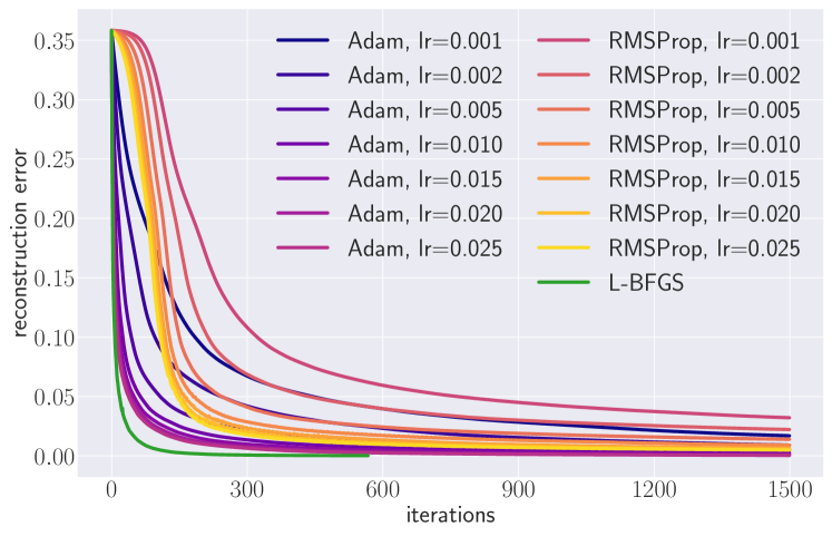
Figure 13. Convergence rate of various optimizers (Adam, RMSProp, L-BFGS) with different learning rates. Mean initialization ($z_{0}=\mu$) is applied in this analysis study.

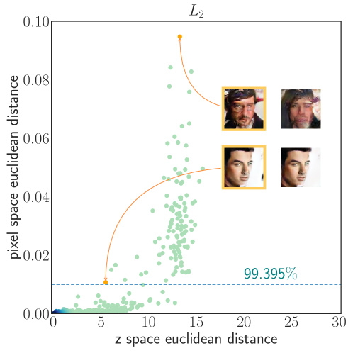
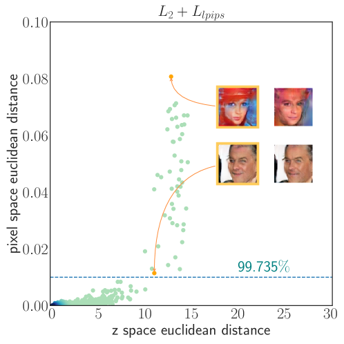
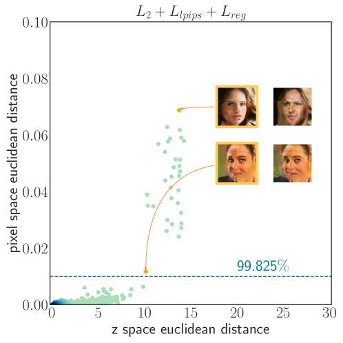
Figure 14. Reconstruction error plots of PGGAN-generated samples on CelebA. The x-axis represents the Euclidean distance between a reconstructed latent code to its ground truth value. The y-axis represents the $L_{2}$ residual in the image domain. The images in orange frame are generated samples. Their reconstructed copies are shown on their right. Samples below the dashed line have reconstruction residuals smaller than 0.01, where no visual difference can be observed. Therefore, the reconstruction is in general better if there is a higher portion of sample points below the dashed line (a higher successful reconstruction rate). (a) Reconstruction results when disabling $L_{\text{lpips}}$ and $L_{\text{reg}}$ ($\lambda_{1}=1.0$, $\lambda_{2}=0$, $\lambda_{3}=0$). (b) Reconstruction results when disabling $L_{\text{reg}}$ ($\lambda_{1}=1.0$, $\lambda_{2}=0.2$, $\lambda_{2}=0$). (c) Reconstruction results when enabling all the $L_{2},L_{\text{lpips}}$ and $L_{\text{reg}}$ terms ($\lambda_{1}=1.0$, $\lambda_{1}=0.2$, $\lambda_{2}=0.001$). We find that using all the terms most benefits the reconstruction.

C.1.3. Analysis on Distance Metric Design for Optimization

We show the effectiveness of our objective design (Section 5.5). Although optimizing only for element-wise difference term $L_{2}$ yields reasonably good reconstruction in most cases, we observe undesired blur in reconstruction for CelebA images. Incorporating deep image feature term $L_{\text{lpips}}$ and regularization term $L_{\text{reg}}$ benefits the successful reconstruction rate. See Figure 14 for a demonstration.

Table 5. Successful reconstruction rate for generated samples from different GANs.

	DCGAN	PGGAN	WGANGP	VAEGAN
Success rate (%)	99.89	99.83	99.55	99.25

C.1.4. Sanity Check on Distance Metric Design for Optimization

In addition, we check if the non-convexity of our objective function affects the feasibility of attack against different victim GANs. We apply optimization to reconstruct generated samples. Ideally, the reconstruction should have no error because the query samples are directly generated by the model, i.e., their preimages exist. We set a threshold of $0.01$ to the reconstruction error for counting successful reconstruction rate, and evaluate the success rate for four GAN models trained on CelebA. Table 5 shows that we obtained more than 99% success rate for all the GANs, which verifies the feasibility of our optimization-based attack.

C.1.5. Analysis on Distance Metric Design for Classification

We propose to enable/disable $\lambda_{1}$, $\lambda_{2}$, or $\lambda_{3}$ in Section 5.5 to investigate the contribution of each term towards classification thresholding (membership inference) on CelebA. In detail, we consider using (1) the element-wise difference term $L_{2}$ only, (2) the deep image feature term $L_{\text{lpips}}$ only, and (3) all the three terms together to evaluate attack performance. Figure 15 shows the AUCROC of attack against each various GANs. We find that our complete distance metric design achieves general superiority to single terms. Therefore, we use the complete distance metric for classification thresholding.

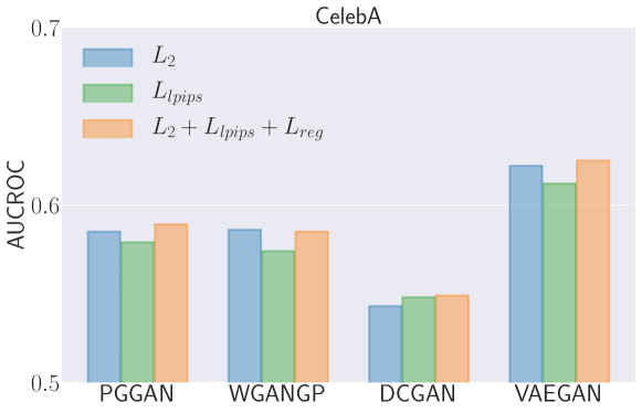
Figure 15. White-box attack performance against GANs on CelebA, w.r.t. distance metric design for classification.

C.2. Additional Quantitative Results

C.2.1. Evaluation on Full Black-box Attack

Attack Performance w.r.t. Training Set Size:  Table 6 corresponds to Figure 5, Figure 5, and Figure 5 in the main paper.

64 128 256 512 1024 2048 4096 20k PGGAN 1.00 1.00 1.00 0.99 0.95 0.79 0.58 0.51 WGANGP 1.00 1.00 1.00 0.97 0.89 0.72 0.62 0.51

(a) CelebA

64 128 256 512 1024 2048 4096 8192 WGANGP 0.98 0.97 0.93 0.87 0.81 0.68 0.54 0.52 MEDGAN 0.78 0.65 0.57 0.54 0.52 0.52 0.51 0.51

(b) MIMIC-III

64 128 256 512 1024 2048 4096 8192 10k WGANGP 1.00 1.00 0.97 0.90 0.72 0.54 0.50 0.50 0.50

(c) Instagram

Table 6. Full black-box attack performance w.r.t. training set size.

Attack Performance w.r.t. Training Set Selection:  Table 7 corresponds to Figure 6 in the main paper.

C.2.2. Evaluation on Partial Black-box Attack

Attack Performance w.r.t. Training Set Selection:  Table 7 corresponds to Figure 6 in the main paper.

PGGAN WGANGP DCGAN VAEGAN random 0.51 0.51 0.51 0.50 identity 0.53 0.53 0.51 0.51

(a) Full black-box

PGGAN WGANGP DCGAN VAEGAN random 0.55 0.53 0.51 0.55 identity 0.57 0.60 0.55 0.58

(b) Partial black-box

PGGAN WGANGP DCGAN VAEGAN random 0.54 0.53 0.52 0.61 identity 0.59 0.59 0.55 0.63

(c) White-box

Table 7. Attack performance on the random v.s. identity-based GAN training set selection. We only focus on CelebA across attack settings.

C.2.3. Evaluation on White-box Attack

Ablation on Distance Metric Design for Classification:  Table 8 corresponds to Figure 15.

DCGAN PGGAN WGANGP VAEGAN $L_{2}$ 0.54 0.59 0.59 0.62 $L_{\text{lpips}}$ 0.55 0.58 0.57 0.61 $L_{2}+L_{\text{lpips}}+L_{\text{reg}}$ 0.55 0.59 0.59 0.63

Table 8. White-box attack performance against various GANs on CelebA, w.r.t. distance metric design for classification.

64 128 256 512 1024 2048 4096 20k PGGAN 1.00 1.00 1.00 0.99 0.95 0.83 0.62 0.55 WGANGP 1.00 1.00 0.99 0.97 0.89 0.78 0.69 0.53

(a) CelebA

64 128 256 512 1024 2048 4096 8192 WGANGP 0.98 0.96 0.92 0.87 0.82 0.80 0.67 0.54 MEDGAN 0.99 0.88 0.77 0.72 0.61 0.59 0.55 0.52

(b) MIMIC-III

64 128 256 512 1024 2048 4096 8192 10k WGANGP 1.00 1.00 0.97 0.90 0.72 0.55 0.50 0.50 0.49

(c) Instagram

Table 9. White-box attack performance w.r.t. training set size.

Attack Performance w.r.t. Training Set Size:  Table 9 corresponds to Figure 5, Figure 5, and Figure 5.

PGGAN WGANGP DCGAN VAEGAN before calibration 0.53 0.53 0.51 0.51 after calibration 0.54 0.54 0.52 0.51

(a) Full black-box

PGGAN WGANGP DCGAN VAEGAN before calibration 0.57 0.60 0.55 0.58 after calibration 0.58 0.63 0.56 0.59

(b) Partial black-box

PGGAN WGANGP DCGAN VAEGAN before calibration 0.59 0.59 0.55 0.63 after calibration 0.68 0.64 0.55 0.76

(c) White-box

Table 10. Attack performance before and after calibration on CelebA.

64 128 256 512 1024 2048 4096 8192 full bb 0.98 0.97 0.93 0.87 0.81 0.68 0.54 0.52 full bb (calibrated) 1.00 0.99 0.97 0.94 0.89 0.84 0.67 0.56 wb 0.98 0.96 0.92 0.87 0.82 0.80 0.67 0.54 wb (calibrated) 0.98 0.97 0.93 0.90 0.87 0.85 0.75 0.59

(a) MIMIC-III (WGANGP)

64 128 256 512 1024 2048 4096 8192 full bb 0.78 0.65 0.57 0.54 0.52 0.52 0.51 0.51 full bb (calibrated) 0.91 0.71 0.63 0.58 0.55 0.53 0.52 0.51 wb 0.99 0.88 0.77 0.72 0.61 0.59 0.55 0.52 wb (calibrated) 0.96 0.87 0.81 0.75 0.65 0.62 0.57 0.55

(b) MIMIC-III (MEDGAN)

64 128 256 512 1024 2048 4096 8192 10k full bb 1.00 1.00 0.97 0.90 0.72 0.54 0.50 0.50 0.49 full bb (calibrated) 1.00 1.00 0.98 0.91 0.80 0.72 0.65 0.57 0.56 wb 1.00 1.00 0.97 0.90 0.72 0.55 0.50 0.50 0.49 wb (calibrated) 1.00 1.00 0.98 0.92 0.79 0.73 0.67 0.58 0.57

(c) Instagram (WGANGP)

Table 11. Attack performance before and after calibration for non-image datasets w.r.t. GAN training set sizes. bb: black-box; wb: white-box.

Attack Performance w.r.t. Training Set Selection:  Table 7 corresponds to Figure 6 in the main paper.

C.2.4. Attack Calibration

Table 10 corresponds to Figure 7 in the main paper. Table 11 corresponds to Figure 8 in the main paper.

C.2.5. Comparison to Baseline Attacks

Table 12 corresponds to Figure 9 in the main paper. Table 13 corresponds to Figure 11 in the main paper. Table 14 corresponds to Figure 10 in the main paper.

PGGAN WGANGP DCGAN VAEGAN VAE full bb (LOGAN) 0.56 0.57 0.52 0.50 0.52 full bb (MC) 0.52 0.52 0.51 0.50 0.51 full bb (ours calibrated) 0.54 0.54 0.52 0.51 0.54 partial bb (ours calibrated) 0.58 0.63 0.56 0.59 0.73 wb (ours calibrated) 0.68 0.66 0.55 0.76 0.94 full (LOGAN/MC) 0.91 0.83 0.83 0.61 0.90

Table 12. Comparison of different attacks on CelebA. bb: black-box; wb: white-box; full: accessible discriminator (full model).

64 128 256 512 1024 2048 4096 8192 full bb (LOGAN) 0.98 0.97 0.96 0.94 0.92 0.83 0.65 0.54 full bb (ours calibrated) 1.00 0.99 0.97 0.94 0.89 0.84 0.67 0.56 wb (ours calibrated) 0.98 0.97 0.93 0.90 0.87 0.85 0.75 0.59 dis (LOGAN) 1.00 1.00 1.00 1.00 1.00 1.00 0.99 0.98

(a) MIMIC-III (WGANGP)

64 128 256 512 1024 2048 4096 8192 full bb (LOGAN) 0.45 0.57 0.53 0.52 0.51 0.52 0.50 0.51 full bb (ours calibrated) 0.91 0.71 0.63 0.58 0.55 0.53 0.52 0.51 wb (calibrated) 0.96 0.87 0.81 0.75 0.65 0.62 0.57 0.55 dis (LOGAN) 1.00 0.92 0.96 0.90 0.85 0.90 0.80 0.73

(b) MIMIC-III (MEDGAN)

64 128 256 512 1024 2048 4096 8192 10k full bb (LOGAN) 1.00 0.99 0.96 0.91 0.68 0.55 0.58 0.55 0.55 full bb (calibrated) 1.00 1.00 0.98 0.91 0.80 0.72 0.65 0.57 0.56 wb (calibrated) 1.00 1.00 0.98 0.92 0.79 0.73 0.67 0.58 0.57 dis (LOGAN) 1.00 1.00 1.00 1.00 1.00 1.00 0.98 0.96 0.93

(c) Instagram (WGANGP)

Table 13. Comparison of different attacks on the other two non-image datasets w.r.t. GAN training set size. bb: black-box; wb: white-box; dis: accessible discriminator.

$k$ 64 128 256 512 1024 2048 4096 8192 15k 20k 40k 60k 80k 100k LOGAN 0.51 0.51 0.51 0.52 0.53 0.53 0.53 0.54 0.55 0.56 0.57 0.58 0.57 0.57 MC 0.50 0.50 0.51 0.51 0.51 0.51 0.52 0.52 0.52 0.52 0.52 0.53 0.53 0.53 ours calibrated 0.51 0.51 0.51 0.52 0.52 0.52 0.53 0.53 0.54 0.54 0.54 0.55 0.55 0.55

Table 14. Full black-box attack performance against PGGAN on CelebA w.r.t. $k$ in Equation 5, the number of generated samples.

C.2.6. Defense

Table 15 corresponds to Figure 12 in the main paper. Table 16 corresponds to Figure 12 in the main paper.

full black-box partial black-box white-box w/o DP 0.54 0.58 0.68 w/ DP 0.53 0.56 0.59

Table 15. Attack performance against PGGAN on CelebA with or without DP defense.

64 128 256 512 1024 2048 4096 white-box w/o DP 1.00 1.00 1.00 0.99 0.95 0.83 0.62 white-box w/ DP 1.00 1.00 0.99 0.98 0.90 0.70 0.56 full black-box w/o DP 1.00 1.00 1.00 0.99 0.95 0.79 0.57 full black-box w/ DP 1.00 1.00 0.99 0.98 0.89 0.68 0.53

Table 16. Attack performance against PGGAN on CelebA with or without DP defense, w.r.t. GAN training set size.

C.3. Additional Qualitative Results

Given query samples $x$, we show their reconstruction copies $R(x|\mathcal{G}_{v})$ and $R(x|\mathcal{G}_{r})$ obtained in our white-box attack.

(a) Query (real) images

(b) PGGAN victim model reconstruction

(c) PGGAN (w/ DP) victim model reconstruction

(d) PGGAN reference model reconstruction

(e) WGANGP victim model reconstruction

(f) WGANGP reference model reconstruction

(g) DCGAN victim model reconstruction

(h) DCGAN reference model reconstruction

(i) VAEGAN victim model reconstruction

(j) VAEGAN reference model reconstruction

Figure 16. Reconstruction of query samples $x$ that are in the training set, i.e., $x\in D_{\text{train}}$.

(a) Query (real) images

(b) PGGAN victim model reconstruction

(c) PGGAN (w/ DP) victim model reconstruction

(d) PGGAN reference model reconstruction

(e) WGANGP victim model reconstruction

(f) WGANGP reference model reconstruction

(g) DCGAN victim model reconstruction

(h) DCGAN reference model reconstruction

(i) VAEGAN victim model reconstruction

(j) VAEGAN reference model reconstruction

Figure 17. Reconstruction of query samples $x$ that are not in the training set, i.e., $x\notin D_{\text{train}}$.