Statistical Assemblies of Particles with Spin

Abstract

Spin, $s$ in quantum theory can assume only half odd integer or integer values. For a given $s$, there exist $n=2s+1$ states $|s,m\rangle$, $m=s,s-1,........,-s$. A statistical assembly of particles (like a beam or target employed in experiments in physics) with the lowest value of spin $s=\frac{1}{2}$ can be described in terms of probabilities $p_{m}$ assigned to the two states $m=\pm\frac{1}{2}$. A generalization of this concept to higher spins $s>\frac{1}{2}$ leads only to a particularly simple category of statistical assemblies known as ‘Oriented systems’. To provide a comprehensive description of all realizable categories of statistical assemblies in experiments, it is advantageous to employ the generators of the Lie group $SU(n)$. The probability domain then gets identified to the interior of regular polyhedra in $\Re^{n-1},$ where the centre corresponds to an unpolarized assembly and the vertices represent ‘pure’ states. All the other interior points correspond to ‘mixed’ states. The higher spin system has embedded within itself a set of $s(2s+1)$ independent axes, which are determinable empirically. Only when all these axes turn out to be collinear, the simple category of ‘Oriented systems’ is realized, where probabilities $p_{m}$ are assigned to the states $|s,m\rangle$. The simplest case of higher spin $s=1$ provides an illustrative example, where additional features of ‘aligned’ and more general ‘non oriented’ categories are displayed .

Dedicated with gratitude to
Dr. C. R. Rao
on the Happy Occasion of his
$100^{th}$ Birthday

With due apologies to the great Telugu poet Bammera Pothana

I Introduction

‘Spin’ brings immediately to mind an object rotating about itself. For eg, the Earth, a spinning top etc. When the spin of the electron was discovered in 1925 by Uhlenbeck and Goudsmit a , two great physicists viz., H A Lorentz (Nobel Laureate, 1902) and Wolfgang Pauli (Nobel Laureate, 1945), who opposed the concept of electron spin, were proved wrong as they had in mind a classical electron with an estimated radius $2.8\times 10^{-13}cm$. To the best of experimental information to date, the electron does not appear to have any size!
‘Spin’ is an intrinsic attribute like mass or electric charge for a particle. Atomic nuclei also have ’spin’, which is essentially the sum total of the intrinsic spins of the nucleons and their orbital angular momenta. The quantum of radiation, viz., the photon also has ’spin’, although it has no mass. In fact, the concept of polarization was first introduced in the context of light. Beams or targets which are essentially statistical assemblies of particles/nuclei with polarized spin are employed in several experiments in physics. We are considering here such statistical assemblies The language used is mostly that of physics due to my lack of knowledge of mathematical terminology employed by experts on probablity theory.

II Quantum Description of Spin

In the quantum description of the submicroscopic world, any observable $A$ associated with a physical system is represented by a bounded linear operator $A$ in a separable Hilbert space ${\cal H}$, which accomodates all possible states $|\psi\rangle$ of the system as vectors in ${\cal H}$. According to the Ehrenfest theorem b , the quantum expectation value

$$\langle A\rangle\equiv\langle\psi|A|\psi\rangle,$$ (1)

represents the classical value of the observable $A$, which indeed satisfies classical laws.
Spin $\vec{S}$, in quantum theory, is defined through the commutation relationships

$$\vec{S}\times\vec{S}=i\hbar\vec{S}$$ (2)

satisfied by its components, $S_{x}=-i\hbar\,G_{yz},$$S_{y}=-i\hbar\,G_{zx}$, $S_{z}=-i\hbar\,G_{xy}$, where $G_{xy}$, $G_{yz}$ and $G_{zx}$ are the generators of the Lie group SO(3) of rotations in the $x-y$, $y-z$ and $z-x$ planes respectively of the real three dimensional physical space. The Lie algebra of this group admits of matrix representations in terms of $n\times n$ matrices, where $n$ is related to the spin, $s$ of a particle through

$$n=2s+1$$ (3)

The electron has spin $s=\frac{1}{2}$. The spin hypothesis a , in the words of Condon and Shortley c ,“quickly cleared up many difficult points, so that it at once gained acceptance”. We use the universally adopted Condon and Shortley phase conventions c . We also employ the natural system of units;

$$\hbar=1,\,c=1$$ (4)

where $\hbar$ symbolizes $\left(2\pi\right)^{-1}$ times the Planck constant $h$ and $c$ denotes the velocity of light. The group SO(3) is homomorphic to the group SU(2) of unitary unimodular $2\times 2$ matrices. For $s=\frac{1}{2}$

$$\vec{S}=\frac{1}{2}\,\vec{\sigma},$$ (5)

where the three components of $\vec{\sigma}$ viz.,

$$\sigma_{x}=\left(\begin{array}[]{cc}0&1\\ 1&0\end{array}\right);\,\sigma_{y}=\left(\begin{array}[]{cc}0&-i\\ i&0\end{array}\right);\,\sigma_{z}=\left(\begin{array}[]{cc}1&0\\ 0&-1\end{array}\right)$$ (6)

are referred to as the Pauli spin matrices.

III Spin States

In general, for any given spin value $s=\frac{1}{2},1,\frac{3}{2},2,....,$there exist a complete orthonormal set of $n$ spin states $|s,m\rangle,$ $m=s,s-1,....,-s$, which are simultaneous eigen states of $S^{2}=\left(\vec{S}.\vec{S}\right)$ and $S_{z}$ such that

$$S^{2}|s,m\rangle=s(s+1)|s,m\rangle,$$ (7)

$$S_{z}|s,m\rangle=m|s,m\rangle,$$ (8)

$$(S_{x}\pm iS_{y})|s,m\rangle=\sqrt{(s\mp m)(s\pm m+1)}|s,m\pm 1\rangle,$$ (9)

if we choose the axis of quantization to be along the $z$-axis of a right handed cartesian co-ordinate system.
In the particular case of $s=\frac{1}{2}$ and $n=2$, the two states

$$|s=\frac{1}{2}\;,\,m=+{\frac{1}{2}}\rangle=\left(\begin{array}[]{cc}1\\ 0\end{array}\right)=\uparrow;\ |s=\frac{1}{2}\;,\,m=-{\frac{1}{2}}\rangle=\left(\begin{array}[]{cc}0\\ 1\end{array}\right)=\downarrow$$ (10)

are referred to as ‘up’ and ‘down’ spin states or spinors. They readily satisfy (7) to (9), as can be seen using (5) and (6). We refer to all values $s\geq$ as higher spins.

IV Density Matrix in Quantum Theory

The elegant concept of the density matrix $\rho$ was introduced by von Neumann and others d , which is ideally suited for our purpose. Any quantum state $|\psi\rangle$, which is a vector in a Hilbert space ${\cal H}$, may be expressed as

$$|\psi\rangle=\sum_{i}C_{i}|\varphi_{i}\rangle,$$ (11)

in terms of a conveniently chosen complete orthonormal set of basis states $\{|\varphi_{i}\rangle\}$ in ${\cal H}$. The complex numbers

$$C_{i}=\langle\varphi_{i}|\psi\rangle,\;C^{*}_{i}=\langle\psi|\varphi_{i}\rangle$$ (12)

are complex conjugates of each other and

$$\sum_{i}{\left|C_{i}\right|}^{2}=1,$$ (13)

for normalized states, $\langle\psi|\psi\rangle=1.$ If,

$$A_{ji}=\langle\varphi_{j}|A|\varphi_{i}\rangle$$ (14)

denote matrix elements of a bounded linear operator $A$ in ${\cal H}$ with respect to the chosen basis, the quantum expectation value (1) of the observable $A$ may be expressed as

$$\langle A\rangle=\langle\psi|A|\psi\rangle=\sum_{i,j}\rho_{ij}A_{ji}=Tr(\rho A)$$ (15)

where $Tr$ denotes trace or spur, while the density matrix $\rho$ is defined through its elements

$$\rho_{ij}=C_{i}C^{*}_{j}=\langle\varphi_{i}|\psi\rangle\langle\psi|\varphi_{j}\rangle$$ (16)

or

$$\rho=|\psi\rangle\langle\psi|$$ (17)

which is hermitian i.e.,

$$\rho^{\dagger}=\rho$$ (18)

The quantum state $\psi$ of the system is thus represented by $\rho$. Moreover,

$$Tr\,{\rho}=1,$$ (19)

which is the same as (13) and

$$\rho^{2}=\rho.$$ (20)

V Spin Density Matrix as a vector in $n^{2}$ Dimensional Linear Vector Space

Identifying the basis states $\{|\phi_{i}\rangle\}$ with the states $\{|sm\rangle\}$ for a particle with spin $s$, we readily see that the spin density matrix $\rho$ is a hermitian $n\times n$ matrix. In general, any complex $n\times n$ matrix may be looked upon as a vector in $n^{2}$ dimensional complex linear vector space of $n\times n$ matrices. If $A$ and $B$ are any two matrices, their inner product $(A,B)$ may be defined through

$$(A,B)=Tr(AB^{\dagger})$$ (21)

so that we may conveniently choose an orthogonal basis $\{\Omega_{0}=1,\Omega_{1},...\Omega_{n^{2}-1}\}$ satisfying

$$Tr(\Omega_{i}\Omega^{\dagger}_{j})=n\,\delta_{ij}$$ (22)

and express $\rho$ in terms of them as

$$\rho=\sum^{n^{2}-1}_{i=0}\omega_{i}\Omega_{i},$$ (23)

where the coefficients

$$\omega_{i}=\frac{1}{n}Tr(\rho\Omega^{\dagger}_{i}),$$ (24)

are complex numbers, in general. The factor $n$ on R.H.S of (22) is to accomodate the unit matrix $\Omega_{0}$ in the chosen basis. As such $\Omega_{1},...\Omega_{n^{2}-1}$ are traceless.
In the particular case of $s=\frac{1}{2},$ the Pauli spin matrices (6) satisfy these criteria and are moreover hermitian, so that the coefficients are real. Thus, we have

$$\rho=\omega_{0}+\vec{\sigma}\cdot\vec{\omega}$$ (25)

where $\omega_{0}=\frac{1}{2}Tr{\rho}=\frac{1}{2}$, using (19) and we may use (5) and (15) to identify

$$\vec{\omega}=\frac{1}{2}Tr({\rho\vec{\sigma}})=\langle\vec{S}\rangle,$$ (26)

as the classical value of spin $\vec{S}$ for particles with $s=\frac{1}{2}$.
It needs to be mentioned that the rows and columns of (6) as well as of the spin density matrix $\rho$, usually, are labelled by the quantum number $m=s,s-1,.....,-s$ in that order. It may be noted that

$$\rho=\left(\begin{array}[]{cc}1&0\\ 0&0\end{array}\right)\;or\;\rho=\left(\begin{array}[]{cc}0&0\\ 0&1\end{array}\right)\,,$$ (27)

if $|\psi\rangle$ itself is $|\frac{1}{2},m\rangle$ with $m=\pm\,\frac{1}{2}$.

VI Statistical Matrix or Density Matrix for A Statistical Assembly of Particles with Spin

A statistical assembly, like a beam or target used in experiments in physics, is essentially a system of a large number $N$ of particles, whose wave functions do not have any spatial overlap. We may define the statistical expectation value for spin $\vec{S}$ in such a system through

$$E(\langle\vec{S}\rangle)=\frac{1}{N}\sum_{i=1}^{N}\langle\vec{S_{i}}\rangle=\frac{1}{N}\sum_{i}^{N}Tr({\rho_{i}\vec{S}})=Tr({\rho}\vec{S})$$ (28)

so that the assembly is characterised by what was referred to as the ‘statistical matrix’ or merely as the density matrix for the statistical assembly

$$\rho=\frac{1}{N}\sum_{i=1}^{N}{\rho_{i}}$$ (29)

and (28) may be referred to as the ‘average expectation value’ of $\vec{S}$. The properties (18) and (19) are valid, but not necessarily (20). The statistical matrix or the density matrix $\rho$ for a statistical assembly may be defined through (29), in general, for any $s$.
In the particular case of $s=\frac{1}{2}$, for example, we have

$$\rho=\frac{1}{2}[1+\vec{\sigma}\cdot\vec{P}]=\frac{1}{2}\left(\begin{array}[]{cc}1+P_{z}&P_{x}-iP_{y}\\ P_{x}+iP_{y}&1-P_{z}\end{array}\right)$$ (30)

where the Polarization Vector, $\vec{P}$ is given by

$$\vec{P}=Tr({\rho}\vec{\sigma})=2E(\langle\vec{S}\rangle)=\frac{1}{N}\sum_{i=1}^{N}2\,\vec{\omega_{i}}$$ (31)

where $\vec{\omega_{i}}$ is given by (26) for each particle $i$.
Moreover, if we consider $N_{\pm}$ particles to be in the $|\frac{1}{2}\pm\frac{1}{2}\rangle$ states respectively, such that $N_{+}+N_{-}=N$, we may use (27) to express ${\rho}$ defined by (29) as

$${\rho}=\frac{1}{N}\left(\begin{array}[]{cc}N_{+}&0\\ 0&N_{-}\end{array}\right)=\left(\begin{array}[]{cc}p_{+\frac{1}{2}}&0\\ 0&p_{-\frac{1}{2}}\end{array}\right)$$ (32)

We may compare (30) and (32), if $P_{x}=P_{y}=0$, when we may identify

$$\frac{N_{\pm}}{N}=\frac{1\pm P_{z}}{2}=p_{\pm\frac{1}{2}}$$ (33)

as the probabilities $p_{m}$ assigned to states with $m=\pm\frac{1}{2}$. Clearly

$${\rho}^{2}\neq{\rho}$$ (34)

for a statistical assembly, except in two extreme cases, viz., either $N_{+}=N$ or $N_{-}=N$, when the statistical assembly is said to be ‘pure’ and ${\rho}^{2}={\rho}$. If $N_{+}=N_{-}$, the statistical assembly is said to be ‘unpolarized’. In all other cases (34) holds and the statistical assembly is said to be ‘mixed’. Thus

$$-1\leq P_{z}=\frac{{N_{+}-N_{-}}}{N}\leq 1$$ (35)

Since $\vec{P}$ is measurable experimentally, ${\rho}$ is determinable empirically and we can take ${\rho}$ given by (30) to the diagonal form (32), with $p_{+{1}/{2}}\geq p_{-{1}/{2}}$, simply by rotating the cartesian coordinate system such that the $z$-axis after rotation is along $\vec{P}$.  ie., the $z$-component of $\vec{P}$ after rotation is $P=|\vec{P}|=\frac{N_{+}-N_{-}}{N}$ ,with $N_{+}\geq N_{-}$ (since L.H.S is positive definite). The assembly is unpolarized if $P=0$, pure if $P=1$ and mixed if $0<P<1$. It may also be noted that

$$\sum_{m}p_{m}=1=M_{0};\hskip 72.26999pt\sum_{m}m\,p_{m}=\frac{1}{2}\;P=M_{1}$$ (36)

are the moments of the probability distribution with respect to $m$.

VII Statistical Assembly of Particles with Higher Spin

Treating $m$ (or equivalently $S_{z}$) as a variate and assigning probablities $p_{m}$ to the states $\left|s,m\right\rangle$, even when $s>\frac{1}{2}$, leads to a particularly simple category of statistical assemblies referred to as ‘oriented’ e and the z-axis w.r.t which the above states are defined through (8) is referred to as the ‘axis of orientation’. Oriented assemblies are characterised by moments

$$M_{k}=\sum_{m}m^{k}p_{m}$$ (37)

of order $k$ going upto $k=n-1=2s$.
In the particular case of polarised assemblies of particles with spin $s=\frac{1}{2}$, the axis of orientation is clearly collinear with $\vec{P}$ and since the most general form (30) for $\rho$ is characterised only by $\vec{P}$, the assembly is always ‘oriented’.
In the case of higher spin $s>\frac{1}{2}$, the general form for ${\rho}$ contains many additional parameters Following Fano f , $\rho$ may be expressed as

$$\rho=\sum_{l=0}^{2s}\sum_{q=-k}^{k}(-1)^{q}\,t_{q}^{k}\,\tau_{q}^{k}\,,$$ (38)

where $\tau_{q}^{k}$ are $k^{th}$ degree homogeneous polynomial in $S_{x}$, $S_{y}$, $S_{z}$. They were referred to originally g as polarized Harmonics and defined by operating the invariant $(\vec{S}.\vec{\nabla})^{k}$ on the solid harmonics ${\cal Y}_{kq}(\vec{r})=r^{k}\,{Y}_{kq}(\theta,\varphi)$ where ${Y}_{kq}(\theta,\varphi)$ denote standard Spherical Harmonics, satisfying the Time Reversal requirement of Wigner h .i.e.,

$$\tau^{k}_{q}=N_{k}(\vec{S}.\vec{\nabla})^{k}r^{k}{Y}_{kq}(\theta,\varphi)\,,$$ (39)

which are irreducible tensors i of rank $k$. The parameters

$$t^{k}_{q}=Tr(\rho\tau^{k}_{q})\,,$$ (40)

in (38) are known as Fano Statistical Tensors. The normalization factor $N_{k}$ in (39) depends not only on $k$ but also on $s$. Instead of the $N_{k}$ originally chosen by Fano f and others j , we shall normalize ${\tau_{q}^{k}}$ differently here, so as to satisfy

$$\left\langle sm^{\prime}\left|{\tau_{q}^{k}}\right|sm\right\rangle=C(sks;mqm^{\prime})[k];\,[k]=\sqrt{2k+1}\,,$$ (41)

which is consistent with k and the later Madison convention l for spin 1 . Making use of the Wigner-Eckart theorem m ; n ; o and denoting the Clebsch-Gordan Coefficients by $C$, we may identify $\sqrt{2k+1}$ as the reduced matrix element $\left\langle s\left|\left|{\tau_{q}^{k}}\right|\right|s\right\rangle$
With the above normalization, it follows that $\tau^{0}_{0}=1$ and

$$Tr[{\tau_{q}^{k}}{\tau_{q^{\prime}}^{\dagger k^{\prime}}}]=n{\delta_{kk^{\prime}}}{\delta_{qq^{\prime}}}\,,$$ (42)

which is akin to (22). Since $q=k,k-1,.....-k$ takes $(2k+1)$ values, it follows that

$$\sum_{k=1}^{2s}(2k+1)=n^{2}-1\,,$$ (43)

which coincides exactly with the number of $\Omega_{i}$, $i=1,....,n^{2}-1$ required in (23). By virtue of Wigner’s definition h of the spherical harmonics $Y_{lm}$ the hermitian conjugate ${\tau_{q}^{\dagger k}}$ of ${\tau_{q}^{k}}$ satisfies

$${\tau_{q}^{\dagger k}}=(-1)^{q}{\tau_{-q}^{k}}\,,$$ (44)

which implies that the complex conjugates $({t_{q}^{k}})^{*}$ of ${t_{q}^{k}}$ are related to $t^{k}_{-q}$ through

$$(t_{q}^{k})^{*}=(-1)^{q}{t_{-q}^{k}}\,,$$ (45)

One may also consider p $\frac{1}{2}[{\tau_{q}^{k}}+(-1)^{q}{\tau_{-q}^{k}})]$ and $\frac{1}{2i}[{\tau_{q}^{k}}+(-1)^{q}{\tau_{-q}^{k}})]$ as independent hermitian $\Omega_{i}$ for (23). Moreover, $t^{k}_{0}$ are real for all $k$. These together with Re ${t_{q}^{k}}$, Im ${t_{q}^{k}}$ for $q>0$ constitute a total of $(n^{2}-1)$ real parameters, apart from ${t_{0}^{0}}=1$. The operators $\tau^{k}_{q}$ as well as the Fano statistical tensors $t^{k}_{q}$, being irreducible tensors of rank $k$, transform under rotations according to

$$(t_{q}^{k})_{II}=\sum_{q=-k}^{k}D^{k}_{q^{\prime}q}(\alpha\beta\gamma)(t_{q^{\prime}}^{k})_{I}\,,$$ (46)

where $(\alpha\beta\gamma)$ denote Euler angles of the rotation from one Cartesian coordinate system $(I)$ to another $(II)$ and $D^{k}_{q^{\prime}q}$ denote elements of the standard rotation matrices m ; n referred to also as Wigner $D$ functions o . In particular

$$\tau^{1}_{q}=\sqrt{\frac{3}{s(s+1)}}S^{1}_{q};\tau^{2}_{q}=\sqrt{\frac{2\times 3\times 5}{s(s+1)(2s-1)(2s+3)}}\,(S^{1}\otimes S^{1})^{2}_{q}\,,$$ (47)

where

$$S^{1}_{0}=S_{z};\hskip 36.135ptS^{1}_{\pm 1}=\mp\frac{1}{\sqrt{2}}(S_{x}\pm iS_{y})$$ (48)

are referred to as the spherical components of $\vec{S}$. They transform, under rotations according to (46) and as such constitute an irreducible tensor of rank $k=1$. The notation

$$(A^{k_{1}}\otimes B^{k_{2}})^{k}_{q}=\sum_{q_{1}}C(k_{1}k_{2}k;q_{1}q_{2}q)A^{k_{1}}_{q_{1}}B^{k_{2}}_{q_{2}}\,,$$ (49)

used in (47) denotes an irreducible tensor of rank $k$ obtained by combining two irreducible tensors $A^{k_{1}}_{q_{1}}$ and $B^{k_{2}}_{q_{2}}$ of ranks $k_{1}$ and $k_{2}$ respectively. Defining k ; l cartesian second rank tensors

$$Q_{\alpha\beta}=\frac{1}{2}[\frac{3}{2}(S_{\alpha}S_{\beta}+S_{\beta}S_{\alpha})-\delta_{\alpha\beta}S^{2}]=\frac{1}{2}{\cal P}_{\alpha\beta};\;\;\alpha,\beta=x,y,z\,$$ (50)

which are symmetric and traceless, we may express

$$(S^{1}\otimes S^{1})^{2}_{0}=\sqrt{\frac{2}{3}}Q_{zz};(S^{1}\otimes S^{1})^{2}_{\pm 1}={\pm\frac{2}{3}}(Q_{xz}\pm iQ_{yz};(S^{1}\otimes S^{1})^{2}_{\pm 2}={\frac{2}{3}}(Q_{xx}-Q_{yy}\pm iQ_{xy}),$$ (51)

so that the Fano statistical tensor $t^{2}_{q}$ may be expressed in terms of the cartesian components

$${P}_{\alpha\beta}=Tr(\rho{\cal P}_{\alpha\beta})$$ (52)

of what is commonly referred to as ’Tensor Polarization’, while $t^{1}_{q}=P^{1}_{q},$ where $P^{1}_{q}$ denote the spherical components of ‘vector polarization’, $\vec{P}$ of a statistical assembly of particles with any arbitrary spin $s$. A cartesian coordinate system with its z-axis parallel to $\vec{P}$ may be referred to as the Lakin q Frame.If an assembly with $\vec{P}\neq 0$ is ‘oriented’, it goes without saying that the axis of orientation must be collinear with $\vec{P}$. It is clear that $t_{q}^{k}$ w.r.t the axis of orientation, should satisfy

$$t^{k}_{q}=B_{k}\delta_{q_{0}}\,,$$ (53)

for an ‘oriented system’, from which it follows that the probablities

$$p_{m}=\frac{1}{2s+1}\sum_{k}C(sks,mom)[k]B_{k}\,,$$ (54)

where

$$B_{k}=[s]G_{k}=\sum_{m}C(sks,mom)[k]p_{m}\,,$$ (55)

have been referred to as ‘Orientation Parameters’ r .
The probablities $p_{m}$ or the moments $M_{k}$ of (37) or the $B_{k}$ or $G_{k}$ of (55) constitute a set of $(n-1)$ real and independent parameters. Together with the polar and azimuthal angles $(\theta,\varphi)$ needed to sepcify teh axis of orientation in space, an ‘oriented’ spin assembly is completely characterised by $(n+1)$ real independent parameters. On the other hand, we have pointed out below (45) that a general analysis of ${\rho}$ shows that one needs a set of $(n^{2}-1)$ real independent parameters to characterise a statistical assembly of particles with spin $s$. Clearly

$$n^{2}-1\geq n+1\,,$$ (56)

where the equality holds only in the case of $n=2$ or $s=\frac{1}{2}$. This shows that when we consider statistical assemblies of higher spin particles, an ‘oriented’ system s constitutes only a particularly simple case, where the $t^{k}_{q}$ are not independent but have $(n^{2}-n-2)$ constraints s . Oriented systems have cylindrical symmetry with respect to the axis of orientation; as such $\rho$ assumes the diagonal form $\rho^{0}$, when the axis of orientation is chosen as the $z$-axis.

VIII Non-Oriented Statistical Assemblies and $SU(n)$ Representation

One can envisage statistical assemblies of particles with higher spin $s>\frac{1}{2}$, which are more general. Such assemblies, with no manifestly cylindrical symmetry, have been named as t as ‘Non-oriented spin systems’; the $\rho$ for these systems cannot be brought to the diagonal form by any suitable choice of the $z$-axis (i.e., the axis quantization).
In such a general case, it is more convenient t to choose, ${\Omega_{i}}$ in (23) as the generators u ; v of the compact semi-simple Lie group $SU(n)$. This group is characterised by $(n-1)$ diagonal matrices $H_{\alpha}$, ${\alpha}=1,....,n-1$ and $(n^{2}-n)$ off-diagonal matrices $E^{\gamma}_{\alpha\beta}$, ${\beta=\alpha+1,...,n}$ and $\gamma=1,2$. Labelling the rows and columns by $\mu,\nu=1,...,n$ these matrices are given in terms of their elements

$$(H_{\alpha})_{\mu\nu}=\left[\frac{n}{\alpha(\alpha+1)}\right]^{\frac{1}{2}}\left\{\begin{array}[]{cc}\delta_{\mu\nu}&\texttt{if}\;\;\,\mu<\alpha+1\\ -\alpha\delta_{\mu\nu}&\texttt{if}\;\;\,\mu=\alpha+1\\ 0&\texttt{if}\;\;\,\mu>\alpha+1\end{array}\right.$$ (60)

$$(E_{\alpha\beta}^{1})_{\mu\nu}=\sqrt{\frac{n}{2}}\,{\delta_{\mu\alpha}}{\delta_{\nu\beta}}=(E_{\alpha\beta}^{1})_{\nu\mu};\;{\nu>{\mu}}$$ (61)

$$(E_{\alpha\beta}^{2})_{\mu\nu}=-i\sqrt{\frac{n}{2}}\,{\delta_{\mu\alpha}}{\delta_{\nu\beta}}=(E_{\alpha\beta}^{2})^{*}_{\nu\mu};\;{\nu>{\mu}}$$ (62)

and are as such hermitian and traceless. They satisfy (22) i.e.,

$$Tr(H_{\alpha}H_{\beta})=n{\delta_{\alpha\beta}}\,,$$ (63)

$$Tr\left(E_{\alpha\beta}^{(\gamma)}E_{\alpha^{\prime}\beta^{\prime}}^{(\gamma^{\prime})}\right)=n{\delta_{\alpha\alpha^{\prime}}}{\delta_{\beta\beta^{\prime}}}{\delta_{\gamma\gamma^{\prime}}}\,,$$ (64)

$$Tr\left(E_{\alpha\beta}^{(\gamma)}H_{\alpha}\right)=0\,.$$ (65)

It may readily be seen in particular that $H_{1}=\sigma_{z},\,E^{1}_{12}=\sigma_{x},\,E^{2}_{12}=\sigma_{y}$ for $n=2$ or $s=\frac{1}{2}$. In the case of $s=1$ or $n=3$, the $H_{\alpha},\,E_{\alpha\beta}^{(\gamma)}$ are given by the eight Gellmann matrices[23]. Thus $(H_{\alpha},E_{\alpha\beta}^{(\gamma)})$ together with the unit matrix $\Omega_{0}=1$ constitute a set of $n^{2}$ linearly independent $n\times n$ matrices and we may express

$$\rho=\frac{1}{n}\left[1+\sum_{\alpha=1}^{n-1}h_{\alpha}H_{\alpha}+\sum_{\alpha=1}^{n-1}\sum_{\beta=\alpha+1}^{n}\sum_{\gamma=1}^{2}e_{\alpha\beta}^{(\gamma)}E_{\alpha\beta}^{(\gamma)}\right]\,,$$ (66)

where the $(n^{2}-1)\;SU(n)$parameters are given, using (60) to (62) in (63) by

$$h_{\alpha}=Tr(\rho H_{\alpha});\;\,e_{\alpha\beta}^{(\gamma)}=Tr\left(\rho E_{\alpha\beta}^{(\gamma)}\right)\,,$$ (67)

and they are real. Note that the hermitian ${\rho}$ can, in general, be brought to the diagonal form $\rho^{0}$, through a unitary transformation represented by the matrix, $U$. If $\rho$ is known in the form (38), in terms of the experimentally determined $t^{k}_{q}$ w.r.t a convinently chosen Laboratory frame ($L$) where the basis states are denoted by $\left|sm\right\rangle_{L}$, we may equate (38) with (63), provided the basis states $\left|\alpha\right\rangle$ of (63) are identified through $\left|\alpha\right\rangle=\left|sm\right\rangle_{L}$, where $\alpha=s+1-m$ takes values $1,2...,n$ as $m$ takes values $m=s,...,-s$. One may then determine the $h_{\alpha}$ in (63) through

$$h_{\alpha}=\frac{1}{\sqrt{n\alpha(\alpha+1)}}\sum_{k}\,[k]\,t_{0}^{k}\left[\sum_{n=0}^{\alpha-1}C(sks;s-n,0,s-n)-\alpha\,C(sks;s-\alpha,0,s-\alpha)\right]\,,$$ (68)

while $e_{\alpha\beta}^{(\gamma)}$ may be determined by equating the real and imaginary parts of

$$e^{(1)}_{{\alpha},{\beta}}+i\,e^{(2)}_{{\alpha},{\beta}}=\frac{\sqrt{2}}{\sqrt{n}}\sum_{k}(-1)^{q}[k]\,C(sks;s+1-\alpha,-q,s+1-\beta)\,t_{q}^{k}\,,$$ (69)

The advantage here is that the $SU(n)$ representation (63) of $\rho$ leads, in general, to the diagonal form

$$\rho^{0}=U{\rho}U^{\dagger}=\frac{1}{n}\left[1+\sum_{\alpha=1}^{n-1}h_{\alpha}^{0}H_{\alpha}\right]\,,$$ (70)

which contains only the $H_{\alpha}$, ${\alpha}=1,....n-1$ and the unit matrix. The eigen states of ${\rho}$ are

$$\left|\alpha\right\rangle_{0}=\sum_{\alpha^{\prime}=1}^{n}U_{\alpha\alpha^{\prime}}\left|\alpha^{\prime}\right\rangle,\;\alpha=1,...,n\,,$$ (71)

while the corresponding eigenvalues are the statistical probabilities

$$p_{\alpha}=\frac{1}{n}\left[1-\sqrt{\frac{n(\alpha-1)}{\alpha}}h^{0}_{\alpha-1}+\sum_{\eta=\alpha}^{n-1}\sqrt{\frac{n}{\eta(\eta+1)}}\,h_{\alpha}^{0}\right],\;\alpha=1,...,n\,,$$ (72)

which add up to 1. The new statistical parameters

$$h_{\alpha}^{0}=\sqrt{\frac{n}{\alpha(\alpha+1)}}\left[\sum_{\eta=1}^{\alpha}p_{\eta}-\alpha p_{\alpha+1}\right],\;{\alpha=1,...n-1}$$ (73)

are sufficiently general to describe oriented as well as non-oriented statistical assemblies.
In the simplest case of an ‘oriented’ assembly, the $\left|\alpha\right\rangle_{0}$ are identifiable as $\left|s,m\right\rangle_{0}$ defined w.r.t the axis of orientation, since $U$ can be identified with a rotation and $U_{\alpha\alpha^{\prime}}=D^{s}_{m^{\prime}m}(\varphi_{0},\theta_{0},0)$ where $(\theta_{0},\varphi_{0})$ define the axis of orientation in the Lab Frame. In the case of ‘non-oriented’ assemblies, one cannot identify all the eigen states $\left|\alpha\right\rangle_{0}$ as eigen states of $S_{z}$, w.r.t any choice of an axis of quantization, since $U$ cannot in this case be identified with a rotation. All rotations are unitary, but not all unitary transformations are rotations when $n>2$.
The second advantage is that one can envisage a correlated inductive procedure to determine the bounds on the $h_{\alpha}^{0}$ for any arbitary spin, noting simply that

$$0\leq p_{\alpha}\leq 1\,,$$ (74)

$$\sum_{\alpha=1}^{n}p_{\alpha}=1\,,$$ (75)

Setting ${\alpha=n-1}$ in (70) and using (72)gives

$$h_{n-1}^{0}=\frac{1}{\sqrt{n-1}}(1-np_{n}).$$ (76)

If $p_{n}=0$, we have the upper limit, while $p_{n}=1$ leads to the lower limit for $h_{n-1}^{0}$. Thus,

$$-\sqrt{n-1}\leq h_{n-1}^{0}\leq\frac{1}{\sqrt{n-1}}.$$ (77)

Setting $\alpha=n-2$ in (70) and using (72) gives

$$h_{n-2}^{0}=\sqrt{\frac{n}{(n-1)(n-2)}}\left[1-p_{n}-(n-1)p_{n-1}\right]\,,$$ (78)

Clearly, the upper limit is realised if $p_{n}=p_{n-1}=0$. If $p_{n}=1$, it is clear that all $p_{\alpha\neq n}=0$, while $p_{n}=0$ allows $p_{n-1}$ to have any value in the range $0\leq p_{n-1}\leq 1$. The lower limit is realised, if $p_{n-1}=1$ (and hence $p_{n}=0$). Thus

$$-\sqrt{\frac{n(n-2)}{n-1}}\leq h_{n-2}^{0}\leq\sqrt{\frac{n}{(n-1)(n-2)}}\,,$$ (79)

it may be noted that $h_{n-2}^{0}=0$, either if $p_{n}=p_{n-1}=\frac{1}{n}$ or if $p_{n}=1$ and hence $p_{n-1}=0$. Setting $\alpha=n-3$ in (70) and using (72) gives

$$h_{n-3}^{0}=\sqrt{\frac{n}{(n-2)(n-3)}}[1-p_{n}-p_{n-1}-(n-2)p_{n-2}]$$ (80)

Clearly the upper limit is realised if $p_{n}=p_{n-1}=p_{n-2}=0$,  while $p_{n-2}=1$ (and hence $p_{n}=p_{n-1}=0$) leads to the lower limit. Thus,

$$\sqrt{\frac{(n)(n-3)}{(n-2)}}\leq h_{n-3}^{0}\leq\sqrt{\frac{n}{(n-2)(n-3)}}$$ (81)

It may be noted that $h_{n-3}^{0}=0$, either if $p_{n}=p_{n-1}=p_{n-2}=\frac{1}{n}$ or if $p_{n}=1$ (and hence $p_{n}=p_{n-2}=0$). We may then set $\alpha=n-4$ and so on. The results obtained may be summerised as

$$\sqrt{\frac{n\alpha}{\alpha+1}}\leq h_{\alpha}^{0}\leq\sqrt{\frac{n}{\alpha(\alpha+1)}};\;\alpha=1,...,n-1$$ (82)

where the upper and lower limits correspond respectively to $p_{n}=p_{n-1}=...=p_{\alpha+1}=0$ and to $p_{\alpha+1}=1$ and hence $p_{n}=p_{n-1}=...=p_{\alpha+2}=0$. Thus, (79) is equivalent to the positivity conditions (71) for $p_{\alpha}$, $\alpha=2,...,n$. Finally the bound $0\leq p_{1}\leq 1$ leads to

$$-1\leq\sum_{\alpha=1}^{n-1}\sqrt{\frac{n}{\alpha(\alpha+1)}}\,h^{0}_{\alpha}\leq n-1\,,$$ (83)

on setting $\alpha=1$ in (67). The structure of the bounds in terms of the $h_{\alpha}^{0}$, $\alpha=1,...,(n-1)$ is valid, in general, for a statistical assembly of particles with any spin, $s$.
More interestingly, we may visualise a real $(n-1)$ dimensional space $\Re^{n-1=2s}$, treating $h_{\alpha}^{0}$, $\alpha=1,...,(n-1)$ as orthogonal coordinates. By setting $p_{\alpha}=0$ in (69) for $\alpha=1,...,n$ leads to a set ${\{S_{\alpha},{\alpha=1},...,n}\}$ of $(n-2)$ dimensional surfaces in $\Re^{n-1}$ enclosing the origin O, which corresponds to $h_{\alpha}=0$, $\alpha=1,...,(n-1)$ and $p_{\alpha}=\frac{1}{n}$, $\alpha=1,...,n$ as is evident from (69). Therefore $p_{\alpha}$ increases from $0$ to $\frac{1}{n}$ as we move along the normal to $S_{\alpha}$ towards the origin, O (while $p_{\alpha}<0$ if we move away from O). Note, moreover, that $p_{\alpha}=1$, $\alpha=1,...,n$ constitute $n$ vertices of a polyhedron inscribed in a hyper sphere of radius $\sqrt{2s}$ in $\Re^{n-1}$. Clearly, the inside of the polyhedron (including its surface) defines the probability domain, where the centre O corresponds physically to an unpolarized statistical assembly and the $n$ vertices correspond to the ‘pure’ states, while all other points inside the polyhedron correspond to ‘mixture’ states of the statistical assembly. The above geometrical visualisation of the probability domain in terms of the $h_{\alpha}^{0}$ is not only elegant, but also valid for any arbitrary $s$. In the simplest case $s=1$ of higher spins, the polyhedron reduces to an equilateral triangle in $\Re^{2}$, as shown in Fig 1.

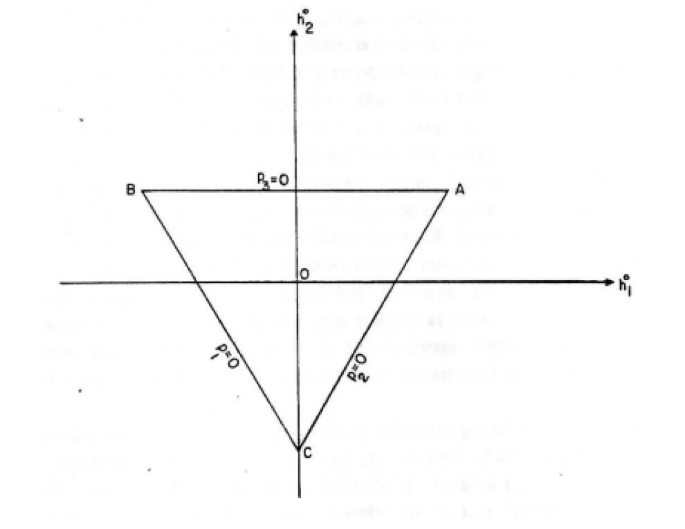
Figure 1: The allowed region for the new statistical tensors $h_{1}^{0}$ and $h_{2}^{0}$ in the case of spin-1 systems. The vertices A, B and C of the equilateral triangle corresponding respectively to $p_{1}=1$, $p_{2}=1$ and $p_{3}=1$ are given by $\left(\sqrt{\frac{3}{2}},\,\sqrt{\frac{1}{2}}\right)$, $\left(-\sqrt{\frac{3}{2}},\,\sqrt{\frac{1}{2}}\right)$ and $\left(0,-\sqrt{2}\right)$ in the $h_{1}^{0}-h_{2}^{0}$ plot.

The bounds in terms of the Fano statistical tensors have been discussed by various authors j ; x in some particular cases like $s=1,\frac{3}{2}$. For $s=\frac{3}{2}$, the discussion in terms of $h_{\alpha}^{0}$ leads to a tetrahedron [20] in $\Re^{3}$, shown in Fig 2.

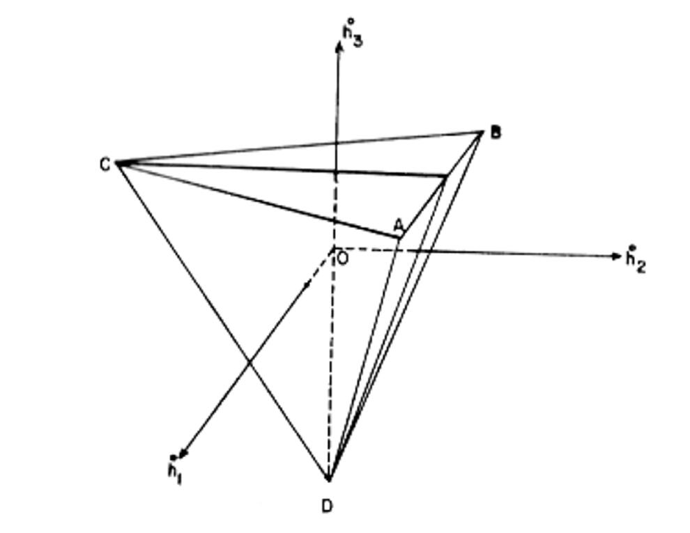
Figure 2: The allowed region for the new statistical tensors $h_{1}^{0}$, $h_{2}^{0}$ and $h_{3}^{0}$ in the case of spin-$\frac{3}{2}$ systems. The vertices A, B , C and D of the regular tetrahedron corresponding respectively to $p_{1}=1$, $p_{2}=1$, $p_{3}=1$ and $p_{4}=1$ are given by $\left(\sqrt{2},\,\sqrt{\frac{2}{3}},\,\sqrt{\frac{1}{3}}\right)$, $\left(-\sqrt{2},\,\sqrt{\frac{2}{3}},\,\sqrt{\frac{1}{3}}\right)$, $\left(0,\,-2\sqrt{\frac{2}{3}},\,\sqrt{\frac{1}{3}}\right)$ and $\left(0,\,0,\,-\sqrt{3}\right)$ in the three dimensional space spanned by $h_{1}^{0},\;h_{2}^{0}$ and $h_{3}^{0}$.

In general, a statistical assembly of particles with spin $s$ may be characterised either in terms of the Fano statistical tensors f or in terms of the $SU(n)$ parameters introduced by Ramachandran and Murthy u , which constitute a total of $(n^{2}-1)$ variates. In either case, the choice of variates is consistent with Gleason’s theorem y .

IX Multiple Axes of Non-Oriented Statistical Assemblies

The richness inherent in non-oriented statistical assemblies of particles with higher spin $s>\frac{1}{2}$, may be appreciated intuitively from the following simple considerations, which is then followed by a formal proof [26]. Any vector $\vec{P}$, such as the one given by (31), may be specified either in terms of its three real components $P_{x},P_{y},P_{z}$ with respect to a given cartesian coordinate system (say Lab) or equivalently by its spherical components.

$$P_{q}^{1}=P\sqrt{\frac{4\pi}{3}}Y_{1q}(\theta,\varphi);\;q=\pm 1,0$$ (84)

in terms of its magnitude $P=\left|\vec{P}\right|$ and direction $\hat{P}=\frac{\vec{P}}{P}$, specified by the angles $(\theta,\varphi)$. Since $P$ is invariant and $P^{1}_{q}$ transform under rotations according to (46), we may envisage an irreducible tensor

$$\hat{P_{0}^{1}}=cos\theta;\hat{P_{\pm}^{1}}=\frac{1}{\sqrt{2}}sin\theta e^{\pm i\varphi}$$ (85)

of rank 1. Clearly, there exists a frame $F$ in which $\hat{P}$ is collinear with the $z$-axis i.e., where $\hat{P}_{\pm}^{1}=0$. We may next envisage an irreducible tensor

$$t_{q}^{2}(1,2)=\left(\hat{P}(1)\otimes\hat{P}(2)\right)^{2}_{q}$$ (86)

of rank 2, constructed out of two given vectors $\vec{P}(1)$ and $\vec{P}(2)$ using (49). Since (83) implies, due to $C(112;\pm 1\pm 1\pm 2)=1$, that $t^{2}_{\pm 2}(1,2)=P_{\pm}^{1}(1)P_{\pm}^{1}(2)$, it follows that there exist two frames $F_{1}$ $F_{2}$ in which $t_{\pm 2}^{2}=0$. Continuing this construction using (49), we may envisage an irreducible tensor

$$t^{k}_{q}(1,...,k)=\left(...((\hat{P}(1)\otimes\hat{P}(2))^{2}\otimes\hat{P}(3))^{3}\otimes...\otimes\hat{P}(k)\right)^{k}_{q}$$ (87)

of any rank $k$ such that $t_{\pm k}^{k}=0$ in $k$ frames $F_{1},F_{2},...,F_{k}$. We may now demonstrate, using (46) and Wigner’s formula i ; m ; o for $D_{q}^{k}(\alpha\beta\gamma)$, that any arbitary irreducible tensor $t_{q}^{k}$ of rank $k$ must indeed be of the form

$$t^{k}_{q}=R_{k}t^{k}_{q}(1,...k)\,,$$ (88)

where $R_{k}$ is an arbitary scalar or real number (like the magnitude $P$ in $\vec{P}=P\hat{P}$) which is invariant with respect to rotations. Given any $t^{k}_{q}$ in a frame $F_{I}$(say Lab), we pose the question: Is there a frame $F_{II}$ w.r.t which $\left(t^{k}_{\pm k}\right)_{II}=0?$ i.e.,

$$\left(t^{k}_{\pm k}\right)_{II}=0=\sum_{q=-k}^{k}D_{q,\pm k}^{k}(\varphi,\,\theta,\,\psi)t_{q}^{k}\,,$$ (89)

where we use $(\varphi,\,\theta,\,\psi)=(\alpha,\,\beta,\,\gamma)$ for the Euler angles in (86), so that $(\theta,\varphi)$ denotes the direction of the $z$-axis of $F_{II}$ with respect to Lab frame $F_{I}$, where the $(2k+1)$ complex numbers $t_{q}^{k}$, $q=k,...,-k$ specify the given irreducible tensor of rank $k$. Using Wigner’s formula i ; m ; o , we may write

$$D_{q,\pm k}^{k}(\varphi\theta\psi)=(a_{\pm})^{2k}\,\left(\begin{array}[]{c}2k\\ k+q\end{array}\right)^{1/2}\,Z_{\pm}^{k+q}$$ (92)

and take $a_{\pm}$ given by

$$a_{+}=sin\frac{\theta}{2}e^{i(\varphi-\psi)/2};\;a_{-}=cos\frac{\theta}{2}e^{i(\varphi+\psi)/2}$$ (93)

out of the summation w.r.t $q$ in (86). The complex variable $Z$ is given by either

$$Z_{+}=cot\frac{\theta}{2}e^{i(\varphi)}\;\;\texttt{or}\;\;Z_{-}=-tan\frac{\theta}{2}e^{i(\varphi)}$$ (94)

so that (86) implies that

$$a_{\pm}=0$$ (95)

or

$$\sum_{q=-k}^{k}C_{q}Z^{k+q}=0$$ (96)

The polynomial equation (91) of degree $2k$ with coefficients

$$C_{q}=\left(\begin{array}[]{c}2k\\ k+q\end{array}\right)^{1/2}\,t_{q}^{k}$$ (99)

yields $2k$ solutions for the complex variable,$Z$. These correspond to $2k$ directions $(\theta_{1},\varphi_{1}),....(\theta_{2k},\varphi_{2k})$ for the $z$-axis of $F_{II}$ w.r.t the Lab frame (where the $t_{q}^{k}$ are given). We may note from (89) that if $(\theta,\varphi)$ is a solution, then $(\pi-\theta,\pi+\varphi)$ is also a solution. This corresponds to the inversion of the $z$-axis of $F_{II}$. It is clear that (90) implies the existence of a pair of solutions, corresponding to $z$-axis of $F_{II}$ being either parallel or antiparallel with the Lab $z$-axis itself. It is worth noting that $\vec{P}$ in (31) is an axial vector or pseudo- vector, whose components $P_{x},P_{y},P_{z}$ remain unaltered under an inversion of the coordinate system (a co-ordinate transformation, which is often referred to in physics as Parity). We therefore conclude that $\vec{P}(1),...,\vec{P}(k)$ considered above must also be axial vectors and that $t_{q}^{k}$ must be of the form (85), which is specified by a set of $k$ axial vectors or Axes. Thus, the $(2k+1)$ real degrees of freedom associated with any irreducible tensor $t_{q}^{k}$ of rank $k$ may be identified with $k$ axes and one real number $R_{k}$, which is essentially a strength factor (akin to $P=|\vec{P}|$) which is invariant under rotations and inversion. Since the density matrix $\rho$ is specified in (38) by $t_{q}^{k}$ with $k=1,...,2s$ the $(n^{2}-1)$ parameters characterising $\rho$ may be identified with

$$N_{A}=\sum_{k=1}^{2s}k=s(2s+1)=sn$$ (100)

axes and $2s=n-1$ real numbers $R_{k}$.
In particular, therefore, a statistical assembly of particles with spin $s=\frac{1}{2}$ is characterised by only one axis viz., $\hat{P}$ and one scalar or real number $P$, as we have already seen in Sec. V. In the case of $s=1$, the statistical assembly is characterised by 3 axes and 2 scalars (or real numbers), which specify respectively the strengths of the vector and tensor polarizations. The number $N_{A}$ of axes increases with $s$. For $s=\frac{3}{2}$, for example, $N_{A}=6$ , while $N_{A}=10$ for $s=2$ and so on. A statistical assembly is ‘oriented’, only when all these $N_{A}$ axes collapse into 1. In the particular case of $s=\frac{1}{2}$, the statistical assembly can only be ‘oriented’, since $N_{A}=1$.

X Particular case of a Non-Oriented Statistical Assembly of Particles with spin $s=1$

It is perhaps appropriate that we take a closer look at the simplest case $s=1$ of a statistical assembly of higher spin particles. In general, the density matrix $\rho$, in this case may be written explicitly as

$${\rho}=\frac{1}{3}\left[\begin{array}[]{ccc}1+\sqrt{\frac{3}{2}}\,t_{0}^{1}+\frac{1}{\sqrt{2}}\,t_{0}^{2}&\;\;\;\sqrt{\frac{3}{2}}\,(t_{-1}^{1}+t_{-1}^{2})&\;\;\;\sqrt{3}\,t_{-2}^{2}\\ \sqrt{\frac{3}{2}}\,(t_{1}^{1}+t_{1}^{2})&\;\;\;1-\sqrt{2}\,t_{0}^{2}&\;\;\;\sqrt{\frac{3}{2}}\,(t_{-1}^{1}-t_{-1}^{2})\\ \sqrt{3}\,t_{2}^{2}&\;\;\;-\sqrt{\frac{3}{2}}\,(t_{1}^{1}-t_{1}^{2})&\;\;\;\;1-\sqrt{\frac{3}{2}}\,t_{0}^{1}+{\frac{1}{\sqrt{2}}}t_{0}^{2}\end{array}\right]$$ (101)

where $t_{q}^{1}=P\hat{P}^{1}_{q}$ as in (81) and (82) and $t_{q}^{2}=R\left(\hat{P}(1)\otimes\hat{P}(2)\right)^{2}_{q}$ as in (83),(85). The assembly is thus characterised by three axes $\hat{P},\hat{P}(1),\hat{P}(2)$ and two scalars Viz, P and R, which represent respectively the strengths of the vector and tensor polarizations. If $P\neq 0$, $R\neq 0$, the assembly is non-oriented, except when all the three axes happen to be collinear. Even if we do away with one axis by setting $P=0$, the statistical assembly in such a case is said to be ‘aligned’, but it is still non-oriented so long as $\hat{P}(1)$ and $\hat{P}(2)$ are distinct. The $t_{q}^{2}$ may explicitly be written as

$$t^{2}_{0}=\frac{R}{\sqrt{6}}[2\,cos{\theta_{1}}cos{\theta_{2}}-sin{\theta_{1}}sin{\theta_{2}}cos({\varphi_{1}}-{\varphi_{1}})]$$ (102)

$$t^{2}_{\pm 1}=\mp\frac{R}{2}[(cos{\theta_{1}}sin{\theta_{2}}cos{\theta_{2}}+cos{\theta_{2}}sin{\theta_{1}}cos{\varphi_{1}}]]\pm i(cos{\theta_{1}}sin{\theta_{2}}sin{\varphi_{2}}+cos{\theta_{2}}sin{\theta_{1}}sin{\varphi_{1}})]$$ (103)

$$t^{2}_{\pm 2}=\frac{R}{2}sin{\theta_{1}}sin{\theta_{2}}[cos({\varphi_{1}}+{\varphi_{1}})\pm isin({\varphi_{1}}-{\varphi_{1}})$$ (104)

in terms of $R,\;\hat{P}(1),\;\hat{P}(2)$. The Fano statistical tensors may also be expressed in terms of the cartesian components $P_{\alpha\beta}$ ;$\alpha,\,\beta=x,y,z$ given by (52) as

$$t^{2}_{0}=\frac{1}{\sqrt{2}}P_{zz}$$ (105)

$$t^{2}_{\pm 1}=\mp\frac{1}{\sqrt{3}}\left(P_{xz}+iP_{yz}\right)$$ (106)

$$t^{2}_{\pm 2}=\frac{1}{2\sqrt{3}}\left(P_{xx}-P_{yy}\pm 2iP_{xy}\right)$$ (107)

Since $P_{\alpha\beta}$ constitute a traceless symmetric second rank Cartesian tensor, one can bring it to the diagonal form $P_{\alpha\alpha}^{0}\delta_{\alpha\beta}$; $\alpha,\beta=x_{A},y_{A},z_{A}$, through a rotation of the coordinate system. The co-ordinate system $\left(x_{A},y_{A},z_{A}\right)$ has been referred to as the Principal Axes of Alignment Frame aa or PAAF for short, where $P_{xy}=P_{yz}=P_{xz}=0$ and consequently $t_{\pm 1}^{2}=0$ and $t_{2}^{2}=t_{-2}^{2}$. Clearly, the two vectors $\vec{P}(1)$ and $\vec{P}(2)$ define a plane. Comparing (98) to (100) respectively with (95) to (97), reveals ab that the plane containing $\vec{P}(1)$ and $\vec{P}(2)$ must be either $z_{A}-x_{A}$ or $x_{A}-y_{A}$ or $y_{A}-z_{A}$ planes where the principal axes $y_{A}$ or $z_{A}$ or $x_{A}$ act as a bisector of the angle between $\vec{P}(1)$ and $\vec{P}(2)$. These cases correspond respectively to the ratio

$$r=\left(\frac{t_{0}^{2}}{t_{2}^{2}}\right)_{PAAF}$$ (108)

being in the intervals $-\infty$ to $-\sqrt{\frac{2}{3}}$, or $-\sqrt{\frac{2}{3}}$ to $\sqrt{\frac{2}{3}}$ or $\sqrt{\frac{2}{3}}$ to $\infty$. The density matrix (94) with $t_{q}^{1}=0$; $t_{\pm 1}=0$ and $t_{2}^{2}=t_{-2}^{2}$ in PAAF may be diagonalized through a Unitary transformation to yield the eigen values

$$p_{x}=\frac{1}{3}\left(1+\frac{1}{\sqrt{2}}t_{0}^{2}+\sqrt{3}t_{2}^{2}\right)$$ (109)

$$p_{y}=\frac{1}{3}\left(1+\frac{1}{\sqrt{2}}t_{0}^{2}-\sqrt{3}t_{2}^{2}\right)$$ (110)

$$p_{z}=\frac{1}{3}\left(1-\sqrt{2}t_{0}^{2}\right)$$ (111)

the corresponding eigen states of $\rho$ being

$$\left|x_{A}\right\rangle=\frac{1}{\sqrt{2}}\left(\left|1,-1\right\rangle_{A}-\left|1,1\right\rangle_{A}\right)$$ (112)

$$\left|y_{A}\right\rangle=\frac{1}{\sqrt{2}}\left(\left|1,-1\right\rangle_{A}+\left|1,1\right\rangle_{A}\right)$$ (113)

$$\left|z_{A}\right\rangle=\left|1,0\right\rangle_{A}$$ (114)

where the eqns (112), (113) and (114) as well as the states $\left|1,m\right\rangle_{A}$ are w.r.t. PAAF. Interestingly, they satisfy

$$S_{\alpha}\left|\alpha\right\rangle=0,\,\alpha=x_{A},y_{A},z_{A}$$ (115)

These three states do not correspond to eigen states of a single operator with different eigen values, but are eigen states of 3 different operators with the same eigen value viz., zero. Labeling the rows and columns by the states defined by (105) to (108), the diagonal form $\rho^{0}$ of $\rho$ is given by

$${\rho}=\frac{1}{3}\left[\begin{array}[]{ccc}1+\sqrt{\frac{3}{2}}\,h_{1}^{0}+\frac{1}{\sqrt{2}}\,h_{2}^{0}&\;\;\;0&\;\;\;0\\ 0&\;\;\;1-\sqrt{\frac{3}{2}}\,h_{1}^{0}+{\frac{1}{\sqrt{2}}}h_{2}^{0}&\;\;\;0\\ 0&\;\;\;0&\;\;\;\;1-\sqrt{2}\,h_{2}^{0}\end{array}\right]$$ (116)

in terms of the $SU(n)$ parameters, so that we readily identify

$$h_{1}^{0}=\sqrt{2}t_{2}^{2};\;\;h_{2}^{0}=t_{0}^{2}$$ (117)

in terms of the $t_{q}^{k}$ in PAAF. It is worth noting that we cannot identify here a single variable like $m$, which was considered as a variate in the case of oriented assemblies.

XI Higher spin particles in final state

Statistical assemblies of particles with spin, $s$ are also produced in experiments when particles collide with each other or with nuclei. We may, in general, consider a collision between $a$ and $b$ producing $c$ and $d$, where $a,b,c,d$ have spins $s_{a},s_{b},s_{c},s_{d}$ respectively and describe the physical process, in quantum theory, by

$$M_{m_{c}m_{d};m_{a}m_{b}}\equiv\left\langle s_{c}m_{c};s_{d}m_{d}\left|M\right|s_{a}m_{a};s_{b}m_{b}\right\rangle\,,$$ (118)

which constitute the elements of a matrix $M$ (with $n_{c}n_{d}$ rows and $n_{a}n_{b}$ columns) at a conserved relativistic energy $E$ (which includes all the masses as well) in a Lorentz frame referred to as c.m. frame (where the conserved total momentum is zero). If $\rho^{a}$ (with $n_{a}$ rows and $n_{a}$ columns) and $\rho^{b}$ (with $n_{b}$ rows and $n_{b}$ columns) denote states of polarization of the beam and target employed initially in the experiment, the final state polarization is described by

$$\rho^{f}=M\rho^{i}M^{\dagger}\,,$$ (119)

where $\rho^{i}$ is the direct product of $\rho^{a}$ and $\rho^{b}$. Due to quantum entanglement, $\rho^{f}$ is not, in general, expressible as a direct product of a $\rho^{c}$ and a $\rho^{d}$. However, if no observations are made on the spin state of say, $d$, one can define the spin state of $c$ by $\rho^{c}$, whose elements are given by

$$\rho^{c}_{m_{c}m_{c^{\prime}}}=\sum_{m_{d}}\rho^{f}_{m_{c}m_{d};m_{c^{\prime}}m_{d}}\,.$$ (120)

After the high energy electron scattering experiments revealed the electromagnetic structure of the nuclei and even of the nucleons themselves, meson factories came up to study their hadronic structure. The meson beams are generated usually through photoproduction or electro-production. Although these experiments were not highly successful in revealing the hadronic structure due to the absence of a theory (for meson scattering) which can make precise quantitative predictions like Quantum Electro Dynamics (which applies in the case of electron and muon scattering). However, improved experimental facilities to study photo- and electro-production of pseudoscalar and vector mesons have become available, with the advent of the new generation of electron accelerators at JLab, MIT, BNL in USA, ELSA at Bonn and MAMI at Mainz in Germany, ESRF at Grenoble in France and Spring8 at Osaka in Japan, with energies going upto 8 GeV. It is, therefore, of interest to allude to photoproduction of $\omega$ mesons (with spin $s=1$), since a theoretical formalism has been developed recently ac , leading to the elegant derivation of formulae for all spin observables associated with the photoproduction of mesons with arbitrary spin-parity . This new theoretical formalism is based on the observation that the ’ket’ and ’bra’ spin states in quantum theory

$$\left|sm\right\rangle=K_{m}^{s};\;\;\left\langle sm\right|=i^{2m}B^{s}_{-m}$$ (121)

transform, under rotations, like irreducible tensors $K_{m}^{s}$ and $B^{s}_{m}$ of rank, $s$ so that one can describe [28] a transistion from an initial state with spin $s_{i}$ to a final state with spin $s_{f}$ through irreducible tensor operators

$$S_{\mu}^{\lambda}(s_{f},s_{i})=i^{2si}[s_{f}]\left(K^{s_{f}}\otimes B^{s_{i}}\right)^{\lambda}_{\mu}$$ (122)

of rank $\lambda=|s_{i}-s_{f}|,....|s_{i}+s_{f}|$. Without going into the details, it is interesting to point out that the $\rho^{\omega}$ of the $\omega$ meson, which is photo or electro produced on protons, can be changed by suitable initial spin preparations of the photon or electron beam and the proton target. Moreover, it is worth being pointed out that the photon, whose spin is 1, has only two states $\left|1,\pm 1\right\rangle$ w.r.t its direction of propagation and these correspond to the right and left circular states of polarization. The absence of the $\left|1,0\right\rangle$ state could be traced (through an analysis of the inhomogeneous Lorentz group, referred to also as Poincare group) to the fact that the mass of the photon is zero. This analysis has also shown that helicity, (which is the component of the spin $\vec{S}$ of a particle along the direction of its momentum and as such is invariant) takes over the role of the magnetic quantum number $m$ in a relativistic theory. The theoretical framework in ac takes all these aspects into consideration and shows for the first time how the reaction matrix elements (111) may be analysed in terms of electric and magnetic multipole amplitudes for the production of mesons with arbitrary non-zero spin $s$. The vector and tensor ae polarizations of the meson are measurable respectively by making use of its decay modes $\omega\rightarrow\pi^{0}+{\gamma}$ and $\omega\rightarrow 3\pi$. It is encouraging to note that the dominant decay mode $\omega\rightarrow 3\pi$ is already being used and experimental work at WASA af is expected to facilitate the use of even $\omega\rightarrow\pi^{0}+{\gamma}$, with the smaller branching ratio of $8.92\%$. The decay of polarised Delta ag with spin 3/2 is another interesting example of current interest in the context of neutral pion production in proton-proton collisions ah

References:

G.E.Uhlenbeck and S.Goudsmit, Naturwiss 13, 953 (1925); Nature 117, 254 (1926)

P.Ehrenfest, Zeits.f.Physik 45, 455 (1927)

E.U.Condon and G.H.Shortley, The Theory of Atomic Spectra (Cambridge Univ. Press, 1935)

J.von Neumann, Nachr.Acad.Wiss Gottingen 1, 245, 273 (1927)
P.A.M.Dirac, Proc. Camb. Phil. Soc. 25, 62 (1929)
L.D.Landau, Z.Phys. 64, 629 (1930)
D.Ter Haar, Rep. Prog. Phys 24, 304 (1961)
W.H.McMaster, Rev. Mod Phys 33, 8 (1961)

R.J.Blinstoyle and M.A.Grace, Handbuch der Physik, Ed:S.Flugge, 62, 555 (Springer Verlag, Berlin, 1957)
J.M.Daniels, Oriented Nuclei (Academic Press, New York, 1965)

U.Fano, National Bureau of Standards, Report 1214 (1951); Phys. Rev. 90, 577 (1953); Rev. Mod. Phys. 29, 74 (1957)

H.Weyl, The Classical Groups (Princeton Univ Press, 1939)
D.L.Falkoff and G.E.Uhlenbeck, Phys. Rev. 72, 322 (1950)

U.Fano and G.Racah, Irreducible Tensorial Sets (Academic press, N.Y. 1959)

E.P.Wigner, Group Theory and its Application to the Quantum Mechanics of Atomic Spectra,
Academic Press, 1959.

M.E.Rose, Phys. Rev. 108, 362 (1957); J. Math. Phys. 3, 408 (1962)
R.H.Dalitz, Ann. Rev. Nucl. Sc. 13, 334 (1963)
P.Minnaert, Phys. Rev. Lett. 16, 672 (1966); Phys. Rev. Lett. 151, 1306 (1966)

G.Ramachandran and R.K.Umerjee, Nucl. Phys. 54, 665 (1964)

G.R.Satchler etal, Proc. III International Symposium on Polarization Phenomena in Nuclear Reactions
Eds.H.H.Barschall%;and W.Haeberli (Univ. of Wisconsin Press, Madison, USA, 1970)

M.E.Rose, Elementary Theory of Angular Momentum (John Wiley, New York, 1957)

G.Ramachandran, Lectures on Angular Momentum, MATSCIENCE Report No 2
(Institute of Mathematical Sciences, Chennai, 1964)

D.A.Varshalovich, A.M.Moskalev and V.K.Khersonski, Quantum Theory of Angular momentum
(World Scientific, 1988)

C.Bourrely, E.Leader and J.Soffer, Phys. Rev. 59, 95 (1980)

W.Lakin, Phys. Rev. Lett. 98, 134 (1955)

K.Siegbahn, Alpha, Beta and Gamma Ray Spectroscopy (North Holland, 1968)

G.Ramachandran and K.S.Mallesh, Nucl. Phys. A 422, 327 (1984)

G.Ramachandran and M.V.N.Murthy, Nucl. Phys. A 302, 444 (1978); Nucl. Phys. A 323, 403 (1979); Nucl. Phys. A 337, 301 (1980)
G.Ramachandran, Non-oriented Spin Systems, Invited Talk at International Symposium on
Perspectives in Nuclear Physics, Madras, 1987

C.Itzykson and M.Nauenberg, Rev. Mod. Phys. 38 95 (1966)
D.B.Lichtenberg, Unitary Symmetry and Elementary Particles (Academic Press, New York, 1970)

G.Racah, Group Theory and Spectroscopy, Lectures delivered at the Institute for
Advanced Study Princeton in Spring%;1951 [CERN Report 61-8]

M.Gellmann, California Institute of Technology Synchrotron Laboratory Report
CTSL 28 (1961) Phys. Rev. $\bf{125}$, 1067 (1963)
M.Gellmann and Y.Neeman, The Eightfold way (Benjamin N.Y. 1965)

G.Ramachandran and K.S.Mallesh, Phys. Rev. C $\bf 40$, 1641 (1989)

A.M.Gleason, Journal of Mathematics and Mechanics $\bf 6$, 855 (1957) V.S.Varadarajan, Geometry of Quantum Theory, II Edition (Springer, Berlin, 1985) K.R.Parathasarathy, An Introduction to Quantum Stochastic Calculus (Birkhauser-Verlag, Berlin, 1992) I.Pitowsky, Quantum Mechanics as a theory of Probablity, arxiv. quant-ph/10510095 (2005)

G.Ramachandran and V.Ravishankar, J. Phys G; Nucl. Phys. $\bf 12$, L143 (1986)

G.Ramachandran, K.S.Mallesh and V.Ravishankar, J. Phys G; Nucl. Phys. (1984)

G.Ramachandran, V.Ravishankar, S.N.Sandhya and Swarnamala Sirsi, J. Phys. G:
Nucl. Phys. $\bf 13$, L271 (1987) V.Ravishankar and G.Ramachandran Phys. Rev. $\bf C35$, 62 (1987)

G.Ramachandran, M.S.Vidya and J.Balasubramanyam, Pramana $\bf 68$, 31 (2007);
Phys. Rev $\bf\;C75$, 065201 (2007)

G.Ramachandran and M.S.Vidya, Invited Talk, Proc. DAE Symp on Nucl. Phys.
Eds:V.M.Datar and S.Kumar $\bf 39A$, 47 (1996); Phys. Rev $\bf\;C56$, R12 (1997)
G.Ramachandran, M.S.Vidya and M.M.Prakash,Phys.Rev $\bf C56$, 2882 (1997)

G.Ramachandran, J.Balasubramanyam, S.P.Shilpashree and G.Padmanabha J. Phys. G;
Nucl. Part. Phys $\bf 34$, 661 (2007)

WASA at COSY Proposal, Ed; B.Hoistad and J.Ritman, arXiv:nucl-ex/0411038 (2004)

G.Ramachandran,  Venkataraya,  M. S. Vidya,  J.Balasubramanyam  and G.Padmanabha  arXiv:0901.0659v1[nucl-th] 6 Jan 2009

Venkataraya,  Sujith Thomas  and  G. Ramachandran   submitted to Phys. Rev. C, 2019