Sustained rotation in a vibrated disk with asymmetric supports

Abstract

A single frictional elastic disk, supported against gravity by two others, rotates steadily when the supports are vibrated and the system is tilted with respect to gravity. Rotation is here studied using Molecular Dynamics Simulations, and a detailed analysis of the dynamics of the system is made. The origin of the observed rotational ratcheting is discussed by considering simplified situations analytically. This shows that the sense of rotation is not fixed by the tilt but depends on the details of the excitation as well.

Keywords: ratcheting, noise rectification, disk packings

1 Introduction

Since the discussion by Feynman of the Feynman-Smoluchowski ratchet in his famous lectures [1], much work has been devoted to the study of ratcheting systems. A system is said to ratchet if it is able to rectify noise (e.g. thermal noise, random vibrations) into directed motion. Examples in microscopic systems can be found in the field of molecular motors [2, 3, 4, 5, 6, 7, 8], while several granular systems have been proposed [9, 10, 11, 12, 13] that display ratcheting on larger size scales. All ratcheting systems work out of equilibrium, which allows them to escape the bounds imposed by the second law of thermodynamics [1, 3].

Symmetry breaking of some sort is a requirement for ratcheting [14, 5]. In granular systems, an asymmetric intruder can be placed in a granular gas. The asymmetries of the embedded object cause an imbalance of collisions that makes this object either move unidirectionally [9, 10], or rotate [11, 12, 13]. Simple systems that rotate can also be conceived [15, 16], in which a chiral rotator is subjected to external excitation.

In this paper, a simple system is studied, that displays rotational ratcheting: a single disk supported by two others against gravity. This system is sketched in Figure 1. When the support disks are vibrated, numerical simulations and experiments [17] show that the upper disk rotates steadily. In our model system, the rotating object is non-chiral, i.e. reflection-symmetric. Reflection symmetry is broken by tilting the system, which causes normal forces at the contacts to differ. The aim of this work is to provide an understanding of the microscopic origin of the rotational phenomenon.

Two rotational regimes can be identified, according to the intensity of the vibration: a regime of gentle driving, where disks never lose contact with each other, and a regime of medium driving, where disks bounce against each other. Although persistent rotation is observed in both dynamical regimes, it results from different dynamical processes in each regime. The case of rotation in the medium driving, bouncing regime, has been already addressed numerically in previous work [17]. The present investigation focuses on the rotational phenomenon for low-intensity driving, that is, in the regime of permanent contacts. In this regime, normal forces between the upper disk and its contacts are never zero, but rotation still happens because of the accumulation of frictional sliding. This regime of sliding rotation is accessible to approximate methods of analysis, which allow one to obtain a basic understanding of the origin of the rotational imbalance. The results of our approximate models can be satisfactorily tested against numerical simulations.

The rest of this paper is organized as follows. In Section 2, the 3-disk model, and the methods used in numerical simulations are introduced. Numerical results showing sustained rotation for random vibration of the supports are presented in Section 3. In Section 4, the origin of the rotational imbalance is discussed, and two approximate models are solved for the simpler case of deterministic periodic excitation of the supports. Finally, our discussion and conclusions are presented in Section 5.

2 Model and Methods

A setup of three disks of radius $R$ is considered, arranged as shown in Figure 1. The freely-moving upper disk is held against gravity by two support disks, whose excitatory motion is externally prescribed, e.g. as periodic or random vibration. Motion of the supports causes fluctuations in the normal $n$ and tangential $\tau$ forces at contacts 1 (left) and 2 (right). Under excitation, and when $\alpha_{1}\neq\alpha_{2}$, the upper disk is found to rotate systematically in a given direction. The system behaves like a ratchet, where the unbiased displacements of the supports are rectified and the angular coordinate of the upper disk $\theta$ drifts with mean rotational velocity ${\bar{\Omega}}$. This velocity ${\bar{\Omega}}$ depends on several parameters, such as: the elastic properties of the disks, the friction coefficient, the vibration intensity, the amount of tilt, and the angle between contacts.

In this paper, the dependence of ${\bar{\Omega}}$ on the vibration intensity $\epsilon_{b}$ and tilt $\theta_{T}$ is explored by means of simulation and approximate modelling. The tilt angle $\theta_{T}$ is defined as the angle between the bisector of the contact lines joining the disk centers and gravity. It can be calculated from the relation $\theta_{T}=(\alpha_{2}-\alpha_{1})/2$, where $\alpha_{1}$ and $\alpha_{2}$ are the contact angles defined in Figure 1. The angle between the contacts was chosen to be $\alpha_{1}+\alpha_{2}=\pi/3$ (see Figure 1), as this is the angle between contacts in the case of a two-dimensional close-packing of equal disks.

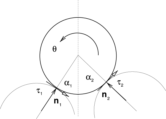
Figure 1: The 3-disk setup showing the direction of normal $n$ and tangential $\tau$ forces. $\theta$ is the angular coordinate of the upper disk. If angles $\alpha_{1}$ and $\alpha_{2}$ are not equal, the upper disk is found to rotate upon vibration of the supporting disks.

For a given prescribed excitatory motion of the support disks, standard molecular dynamics simulations were performed in order to follow the movements of the upper disk. The equations of motions were integrated using a fifth-order predictor-corrector algorithm [18] with a time-step $dt=1{\times}{10^{{-6}}}$. Each simulation ran up to $5\times 10^{8}$ time-steps for constant conditions.

2.1 Normal forces

In our work, linear elasticity is assumed for the normal force between two disks with centers at $\vec{r}_{a}$ and $\vec{r}_{b}$ with radii $R_{a}$ and $R_{b}$. Defining $\delta=(R_{a}+R_{b})-|\vec{r}_{b}-\vec{r}_{a}|$, one has

$$\vec{n}=\hat{n}_{ab}\left(k_{n}\delta-\gamma_{n}u_{n}\right),$$ (1)

where $\hat{n}_{ab}$ is the normal versor, $k_{n}$ is the compressive elastic constant, $\gamma_{n}$ is a viscous constant, and $u_{n}$ is the normal relative velocity (any sign) between disks. The viscous term $\gamma_{n}u_{n}$ accounts for the energy dissipated through viscoelastic deformations of the disks. Notice that (1) can become negative for two disks that are still “in contact” (the distance betewen their centers is smaller than the sum of their radii), if they are moving appart from each other fast enough, because in this case the contribution from the viscosity term is negative. Not correcting for this would be unphysical, since, by definition, normal forces can only be compressive. In a correct implementation of visco-elastic forces, one thus replaces (1) with

$$\vec{n}=\hat{n}_{ab}\ \rm{max}\left(k_{n}\delta-\gamma_{n}u_{n},\ 0\right).$$ (2)

The physical meaning of this “cutoff” is easy to explain. When two visco-elastic disks that are compressed toghether start to move apart, it takes a certain time for them to expand and regain their original shape. Therefore, if their (negative) relative velocity is large enough, they can become detached from each other (their normal force becomes zero) even before the distance between their centers becomes larger than the sum of their radii.

2.2 Tangential forces

A number of proposals have been put forward [19, 20, 21, 22, 23, 24] to describe frictional forces between elastic bodies. The model for tangential forces that is used in this work is a slightly modified form of one originally proposed by Cundall and Strack [19, 25]. An “elastic skin” with tangential stiffness $k_{t}$ accounts for tangential forces at each closed contact. The tangential force is defined to be

$$\vec{\tau}=-k_{t}\delta_{t}\hat{t}_{ab},$$ (3)

where $\hat{t}_{ab}$ is the tangential versor, and $\delta_{t}$ is the accumulated tangential relative displacement between disks since they last came in contact with each other.

The total tangential force is furthermore limited by the Amonton condition

$$\left|\tau\right|\leq\mu n.$$ (4)

If the Amonton condition is violated, $\delta_{t}$ is modified in order to keep the total tangential force right at the frictional limit. This adaptation represents the dissipative loss of elastic energy stored in the “elastic skin”, i.e., the particle’s skin “slips” whenever Amonton’s limit is reached.

In the original model by Cundall and Strack [19], $\delta_{t}$ is calculated as the time integral of the relative tangential velocity of the surfaces in contact. This method of calculating $\delta_{t}$ has been shown to cause unrealistic deformation and ratcheting in granular packings [26], caused by an artificial path dependence of the potential energy stored in the elastic skin. Here an alternative, less error-prone, procedure was implemented. This procedure allows one to calculate $\delta_{t}$ exactly, directly from the knowledge of particle coordinates at time $t$, plus one additional quantity that stores the memory of the first contact and is modified upon sliding.

Let $\theta_{a}$ be the angular coordinate of a disk $a$. Upon general rotations and displacements of their centers, the relative tangential displacement $\lambda_{ab}$ of two disks $a$ and $b$ in contact is given by

$$\lambda_{ab}=R_{a}\theta_{a}+R_{b}\theta_{b}-\beta_{ab}(R_{a}+R_{b}),$$ (5)

where $\beta_{ab}$ is the angle made by the line that joins the centers of the disks in contact with the $x$-axis. Notice that $\lambda$ is constant for two disks that roll on each other rigidly (without deformation of the skin) and without slippage.

Assume that, when two disks are put in contact, their relative tangential coordinate equals $\lambda^{*}$. If these disks are now moved slightly with respect to each other, producing a change in $\lambda$ (without slip), tangential forces will develop. Tangential forces in our model were already defined to depend linearly on the deformation of the skin [19], that is:

$$\tau=-k_{t}(\lambda-\lambda^{*}),$$ (6)

where it was assumed that no skin “slippage” has occurred as a consequence of the tangential deformation. Therefore, upon stretching of the skin, $\lambda^{*}$ still has the value that was defined at first contact. When the tangential force is large enough to violate Amonton’s condition, the skin “slides” or “slips”. This is represented, in our implementation, by a change in $\lambda^{*}$ for that contact, so as to maintain $|\tau|$ at its maximum possible value, which is given by $\mu n$.

By way of example, assume that the Amonton condition is violated, resulting in $-\mu n>k_{t}(\lambda-\lambda^{*})$. In this case, one redefines $\lambda^{*}=\lambda+\mu n/k_{t}$, such that the equality $-\mu n=k_{t}(\lambda-\lambda^{*})$ is restored. If, on the other hand, the violation of the Amonton condition is such that $k_{t}(\lambda-\lambda^{*})>\mu n$, one redefines $\lambda^{*}=\lambda-\mu n/k_{t}$ so as to have $k_{t}(\lambda-\lambda^{*})=\mu n$. This defines a sliding event, which simply amounts to a shift in $\lambda^{*}$.

3 Results for randomly vibrating supports

While it is possible to numerically devise different displacement schemes for the support disks, random vibration is of primary interest, as it demonstrates the noise rectification properties of the system. In this section, numerical results for such case are presented. Later, in Sections 4.1 and 4.2, numerical results for deterministic motion of the supports will be presented, along with an analytic description of the dynamics.

For numerical simulations reported here, gravity was set to $g=10$ and disks were given a radius of $R=1$ and a mass $m=0.1$. This results in a gravitational force of $mg=1$. Units are arbitrary. Since our goal is to analyze the rotational phenomenon and its causes, no attempt to relate the simulated system to a physical one is made in this study.

Other physical constants can be related to the three quantities just introduced as follows: With the given values for $g$, $R$, and $m$, the normal stiffness $k_{n}$ can be defined from the ratio of the force required to compress a disk to half is size and the force due to gravity, ${k_{n}R}/{mg}$. Since $R/mg=1$, this ratio is exactly equal to $k_{n}$. Similarly, $k_{t}$ is the ratio of the force needed to obtain a tangential displacement of one radius and the force due to gravity, ${k_{t}R}/{mg}=k_{t}$.

Numerical simulations were performed with a normal stiffness of $k_{n}=1{\times}{10^{{3}}}$, tangential stiffness of $k_{t}=1{\times}{10^{{6}}}$, viscous damping $\gamma=10$, and friction coefficient $\mu=0.1$. Stiffness values where chosen to make the disk tangentially stiff, while being relatively soft in the normal direction. This allows us to explore a wider range of excitation amplitudes, without the disk losing contact with the supports. Viscous dissipation is chosen to keep normal oscillations in the underdamped regime, as it corresponds to a damping ratio of $\gamma/2\sqrt{k_{n}m}=0.5$.

It is also useful to define a characteristic time for the system. The time needed for a disk to move a distance of one radius, starting from repose and under the effect of gravity, is $t_{g}=\sqrt{2R/g}=1/\sqrt{5}$. This way, given a mean rotational velocity ${\bar{\Omega}}$, the quantity ${\bar{\Omega}}t_{g}$ is the angle rotated during a time interval of $t_{g}$.

Random vibration is implemented by assuming that the coordinates $x$, $y$ and $\theta$ of each support disk follow the dynamics of a white-noise-forced harmonic oscillator. For example, for the $x$ coordinate, the following stochastic equation of motion is integrated:

$$\ddot{x}(t)+2c\omega\dot{x}(t)+\omega^{2}x(t)=\xi(t),$$ (7)

where $c$ is the damping ratio, $\omega$ is the natural frequency of oscillation, and $\xi(t)$ is the forcing term. The random acceleration $\xi(t)$ has mean $\left<\xi(t)\right>=0$ and correlation $\left<\xi(t)\xi(t^{\prime})\right>=4c\omega^{3}{(\epsilon_{b}R)}^{2}\delta(t-t^{\prime})$, where $\epsilon_{b}R$ is the root mean square displacement of the vibration, and $\epsilon_{b}$ is a dimensionless parameter controlling the amplitude of this displacement with respect to the disk radius $R$. The motion of the support disks is continuous and has a correlation time of $t_{c}=1/c\omega$ [27]. The values for the damping ratio and the natural frequency of the vibration were set to $c=0.5$ and $\omega=20\pi$. The ratio of the correlation time $t_{c}$ to the characteristic time $t_{g}$ is $t_{c}/t_{g}=\sqrt{5}/c\omega\approx 0.07$.

Figure 2 shows the scaled mean angular velocity $t_{g}{\bar{\Omega}}$ of the upper disk vs $\epsilon_{b}$ for several values of tilt $\theta_{T}$. For $\theta_{T}=0$, the disk does not rotate, as expected since the system is reflection-symmetric in this case.

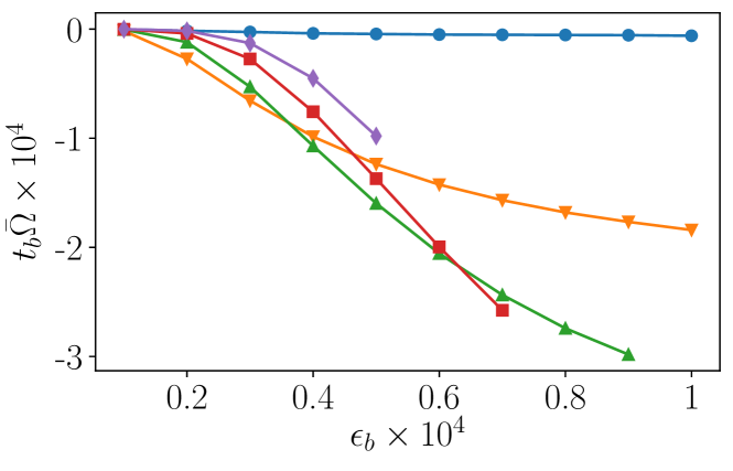
Figure 2: Numerical simulation results for the scaled mean rotational velocity $t_{b}{\bar{\Omega}}$ of the upper disk vs the scaled RMS amplitude $\epsilon_{b}$ of the vibrating support disks. Different lines correspond to different values of system tilt with respect to gravity, $\theta_{T}=0\pi$ (circles), $\theta_{T}=0.02\pi$ (triangles pointing down), $\theta_{T}=0.04\pi$ (triangles pointing up), $\theta_{T}=0.06\pi$ (squares), $\theta_{T}=0.08\pi$ (diamonds).

In Figure 3 the scaled angular velocity $t_{b}{\bar{\Omega}}$ is shown vs the system tilt $\theta_{T}$, for several values of the scaled amplitude $\epsilon_{b}$. The rotational velocity is always clockwise (negative), and there is a non-monotonic dependence of ${\bar{\Omega}}$ on $\theta_{T}$.

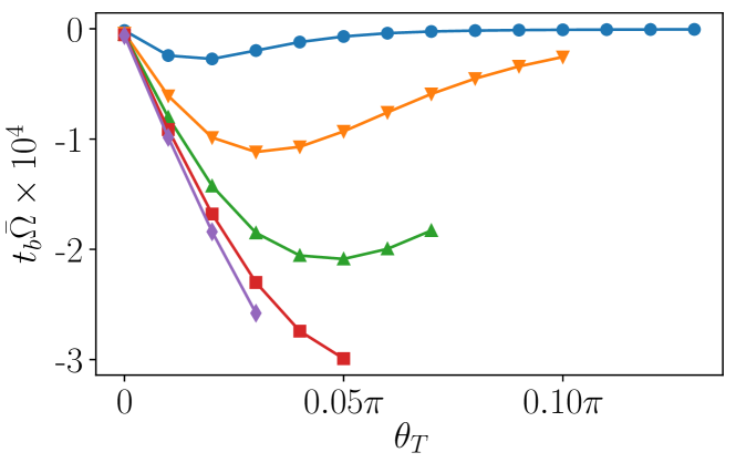
Figure 3: Numerical simulation results for the scaled mean rotational velocity $t_{b}{\bar{\Omega}}$ of the upper disk vs the system tilt $\theta_{T}$. Different lines correspond to different values of amplitude $\epsilon_{b}$ of the support vibrations, $\epsilon_{b}=2{\times}{10^{{-5}}}$ (circles), $\epsilon_{b}=4{\times}{10^{{-5}}}$ (triangles pointing down), $\epsilon_{b}=6{\times}{10^{{-5}}}$ (triangles pointing up), $\epsilon_{b}=8{\times}{10^{{-5}}}$ (squares), $\epsilon_{b}=1{\times}{10^{{-4}}}$ (diamonds).

In all simulations presented here, the upper disk never loses contact with the supports. These results thus show that when the system is tilted, the breaking of left-right symmetry allows the upper disk to rotate systematically in a given direction. In the next section we explore in more detail how this asymmetry induces rotation without assuming any particular displacement scheme for the supports.

4 Analysis of the dynamics of rotation

In this Section, the microscopic mechanisms that cause rotation in the 3-disk system are explored. Before starting such analysis, it is useful to describe the relation between our 3-disk system and a one-dimensional system subjected to similar frictional constraints, that also exhibits drift under random excitation, namely the elasto-plastic oscillator (EPO).

A model for the undamped EPO is displayed in Figure 4. It consists of an externally excited mass $m$, coupled to a linear spring in series with a frictional slip-joint. Due to the fictional slip-joint, the force-displacement response of the EPO is non-linear. Whenever the magnitude of the force on the spring reaches a predefined threshold, the joints slide and the force remains constant. The response of the EPO (and its generalizations) to both harmonic forcing [28, 29, 30, 31, 32, 33, 34, 35, 36, 37, 38, 39, 40, 41] and random forcing [42, 43, 44, 45, 46, 47, 48, 49, 50, 51, 52] has been extensively studied before.

Figure 4: The undamped elasto-plastic oscillator. An externally excited mass $m$ coupled to a linear spring, of stiffness $k$, in series with a frictional slip-joint. The joint slides whenever magnitude of the force at the spring reaches a threshold value.

Figure 5 shows a possible force-displacement response for the asymmetric EPO, starting at the equilibrium position at $x=0$. Under the effect of the forcing, the mass starts to move in the positive direction, and the force $F$ changes linearly, moving towards $F_{1}$. At the limit $F_{1}$, the slip-joint starts sliding. As the mass continuous sliding, the force is kept constant at $F_{1}$. Eventually, the direction of motion is reversed, and the joint stops sliding. The force behaves linearly again and starts increasing towards $F_{2}$. Upon reaching $F_{2}$, the joint slides again and the force remains constant until motion once again reverses direction. Notice that, after sliding, the equilibrium point has been displaced by an amount equal to the net sliding distance, the force crossing zero at different values for $x$. When the forcing cycle ends, the oscillator has experienced a positive drift.

Whenever the slip-joint slides, the equilibrium position moves in the direction of sliding. If the frictional limits of the EPO are symmetric, i.e., if $\left|F_{1}\right|=\left|F_{2}\right|$, sliding is equally likely in either direction. The EPO experiences normal diffusion [51], and its displacement averages to zero. If, on the other hand, $\left|F_{1}\right|\neq\left|F_{2}\right|$, sliding will be biased towards the smaller threshold. In this case, the mass will drift systematically due to net sliding displacements in one direction being larger than in the other. For example, if $F_{1}<F_{2}$, the mass slides more often to the right, making the average velocity of the EPO positive. Such a drift has been studied in [41] for a harmonically forced EPO, and in [50] for random forcing.

Figure 5: A possible evolution of the force on the spring in the EPO (Figure 4). The force changes linearly with displacement as long as $F_{1}<F<F_{2}$. Once either limit is reached the force remains constant. If $F_{1}<F_{2}$, the lower limit is reached more easily, leading to a systematic displacement of the equilibrium point of the oscillator.

Each contact of the 3-disk system behaves similarly to an EPO. Whenever the relative tangential displacement of the upper disk and the support reaches the limit imposed by the Amonton condition (equation (4)), the contact slides. If sliding is biased, the upper disk rotates systematically upon being excited. The system can be rationalized as two slip-joints, one at each contact, which are rigidly coupled to each other. This coupling makes the 3-disk system notably harder to analyze than the EPO. Additionally, the Amonton limits for different directions of sliding are not fixed, because normal forces at each contact are allowed to change in response to the relative displacement of the disks.

The forces acting on the disk are the normal and tangential forces at the contacts, written as $n_{i}$ and $\tau_{i}$ for contact with the support disk $i$, where $i=1,2$. Newton’s second law applied to the upper disk’s center of mass results in the equations of motion:

$$m\ddot{x}=n_{1}\sin\alpha_{1}-n_{2}\sin\alpha_{2}+\tau_{1}\cos\alpha_{1}+\tau_{2}\cos\alpha_{2}$$ (8)

$$m\ddot{y}=n_{1}\cos\alpha_{1}+n_{2}\cos\alpha_{2}-\tau_{1}\sin\alpha_{1}+\tau_{2}\sin\alpha_{2}-mg,$$ (9)

where $x$ and $y$ are the coordinates of the upper disk’s center, $m$ is the upper disk’s mass, $g$ is the gravitational acceleration, and the angles $\alpha_{1}$ and $\alpha_{2}$ are defined in Figure 1.

Similarly, the total torque on the upper disk, caused by tangential forces $\tau_{1}$ and $\tau_{2}$, is given by

$$\mathcal{T}=R_{0}(\tau_{1}+\tau_{2}),$$ (10)

where $R_{0}$ is the upper disk’s radius.

Normal and tangential forces depend on the relative distance between the upper disk and the supports (see Section 2), making equations (8) trough (10) a set of coupled differential equations. The system is non-linear because tangential forces, which are subjected to the Amonton condition, introduce a discontinuity into the equations each time a contact slides or ceases sliding. This makes the equations of motion hard to solve, and motivates the introduction of the following approximation to make the system tractable. In the regime of large support displacements and low friction coefficient $\mu$, it is expected that contacts will remain sliding most of the time. It is reasonable, then, to ignore the duration of elastic deformations of the tangential skin and assume that contacts are always sliding. From now on, this assumption will be referred as the permanent-sliding approximation. The assumption is the opposite of the one usually made in analytical treatments of the EPO. For the EPO, it is often assumed (see, for example, references [43, 50, 49]) that the slip-joint rarely slides, such that the dynamics of the elastic regime is dominant. In the numerical simulations reported in Section 3, it was verified that contacts slide most of the time, in accordance with the proposed approximation. In alternative simulations (not shown), where the supports move with low intensity and sliding is rare, sustained rotation of the upper disk was never observed numerically.

Under the assumption of permanent sliding, Amonton’s equation (4) becomes an equality, and can be used to reduce the number of unknowns by rewriting equations (8) and (9) in a form that only involves tangential forces,

$$\mu m\ddot{x}=\left|\tau_{1}\right|\sin\alpha_{1}-\left|\tau_{2}\right|\sin\alpha_{2}+\mu\tau_{1}\cos\alpha_{1}+\mu\tau_{2}\cos\alpha_{2}$$ (11)

$$\mu m\ddot{y}=\left|\tau_{1}\right|\cos\alpha_{1}+\left|\tau_{2}\right|\cos\alpha_{2}-\mu\tau_{1}\sin\alpha_{1}+\mu\tau_{2}\sin\alpha_{2}-mg.$$ (12)

The absolute values in equations (11) and (12) can be split into four different cases, depending on the signs of $\tau_{1}$ and $\tau_{2}$. Each of these four cases can be identified with a different sliding configuration of contacts in the 3-disk system. These configurations are referred to as $\{S^{++},S^{--},S^{+-},S^{-+}\}$. At $S^{++}$, both contacts are sliding clockwise, and tangential forces are both positive. At $S^{--}$, both contacts are sliding counter-clockwise, and tangential forces are negative. At $S^{+-}$, contact 1 is sliding clockwise ($\tau_{1}>0)$ and contact 2 is sliding counter-clockwise ($\tau_{2}<0$). Finally, at $S^{-+}$, contact 1 is sliding counter-clockwise ($\tau_{1}<0)$ and contact 2 is sliding clockwise ($\tau_{2}>0$).

For example, for configuration $S^{++}$, for which both tangential forces are positive, the following equations of motion are obtained:

$$\mu m\ddot{x}=(\sin\alpha_{1}+\mu\cos\alpha_{1})\tau_{1}-(\sin\alpha_{2}-\mu\cos\alpha_{2})\tau_{2}$$ (13)

$$\mu m\ddot{y}=(\cos\alpha_{1}-\mu\sin\alpha_{1})\tau_{1}+(\cos\alpha_{2}+\mu\sin\alpha_{2})\tau_{2}-mg.$$ (14)

Similar equations are obtained for the other three sliding configurations.

Within the permanent sliding approximation, and since the duration of elastic deformations is neglected, the dynamics of the system can be approximated as series of transitions between these four sliding configurations. Transitions between configurations occur each time the direction of sliding is reversed at a contact. At the moment of this reversal, the velocity of the upper disk and the support become equal. In practice, sliding stops momentarily, and a period of elastic deformation of the skin begins. For the permanent-sliding approximation to remain valid, this period of elastic deformation needs to be much shorter than a typical duration of a sliding configuration. If support disks move tangentially with a velocity much larger than the rotational velocity of the upper disk this condition is met.

Assume the system, on average, stays at each sliding configuration $S^{\pm\pm}$ during a time interval $T^{\pm\pm}$. The net angular displacement that the upper disk undergoes in such interval can be obtain from the average torque $\bar{\mathcal{T}}^{\pm\pm}$ acting on the disk during $T^{\pm\pm}$.

Equations (11) and (12) can be used to estimate $\bar{\mathcal{T}}^{\pm\pm}$. Unlike equations (8) and (9), equations (11) and (12) have a well defined translational-equilibrium solution (solutions for which ${\mathop{x}\limits^{\vbox to-1.4pt{\kern-2.0pt\hbox{...}\vss}}}=\ddot{y}=0$). In general, the equilibrium solution for the 3-disk system is not unique, the solution involves solving a system of 3 equations of motion with four unknown forces (see [53] for a more detailed discussion). But, once sliding is assumed at both contacts, equations (11) and (12) become a system of two equations with two unknowns, from which equilibrium tangential forces $\tau_{1}^{eq}$ and $\tau_{2}^{eq}$ can be obtained. For example, for configuration $S^{++}$, equilibrium tangential forces can be obtained by setting $\ddot{x}=\ddot{y}=0$ in equations (13) and (14) and solving the resulting system. Plugging the solutions into equation (10) yields the equilibrium torque

$$\mathcal{T}_{eq}^{++}=\frac{mgR\mu(\cos\theta_{T}+\mu\sin\theta_{T})}{(1+\mu^{2})\cos\theta_{h}},$$ (15)

where $\theta_{T}$ is the tilt angle, defined is Section 2 as $\theta_{T}=(\alpha_{2}-\alpha_{1})/2$, and $\theta_{h}$ is half the aperture angle of the contacts, defined as $\theta_{h}=(\alpha_{2}+\alpha_{1})/2$. Similarly, the equilibrium torques for configurations $S^{--}$, $S^{+-}$, and $S^{-+}$ are obtained as

$$\mathcal{T}_{eq}^{--}=-\frac{mgR\mu(\cos\theta_{T}-\mu\sin\theta_{T})}{(1+\mu^{2})\cos\theta_{h}}$$ (16)

$$\mathcal{T}_{eq}^{+-}=\frac{mgR\mu\sin\theta_{T}}{\sin\theta_{h}+\mu\cos\theta_{h}}$$ (17)

$$\mathcal{T}_{eq}^{-+}=-\frac{mgR\mu\sin\theta_{T}}{\sin\theta_{h}-\mu\cos\theta_{h}}.$$ (18)

The equilibrium points just discussed are not true dynamical equilibrium points, since the total torque on the upper disk is not zero. At these points, the center of the upper disk is assumed in equilibrium, but there is angular acceleration caused by the torque $\mathcal{T}_{eq}^{\pm\pm}$. We define these points to be translational equilibrium points, or TEPs. Each TEP is defined by the point towards which the disk center is assumed to evolve at $S^{\pm\pm}$. For example, consider the case of support disks moving only tangentially to the contact point (or only rotating). If the system stays at configuration $S^{\pm\pm}$ long enough, the transient initial state will dissipate, and the dynamics will converge to the TEP. We are assuming here that fluctuations around equilibrium will dissipate due to damping forces. In the more general case, at which normal displacements are not restricted, fluctuations around the TEP will not cease. Nevertheless, the TEP point will still be an attractor of the dynamics. This statement can be justified by relaxing the constraints, and, instead of dynamical equilibrium ($\ddot{x}=\ddot{y}=0$), only statistical stationarity needs to be assumed. This is, we replace all quantities in equations (11) and (12) by their mean values, and require that the mean accelerations vanish, $\ddot{\bar{x}}=\ddot{\bar{y}}=0$. In this case, the TEP defines the mean values for contact forces around which fluctuations take place.

Consider the following case to illustrate the nature of the TEP: Assume supports are rotating clockwise, much faster than the upper disk, with both contacts sliding at configuration $S^{++}$. After some time, any oscillatory dynamical behavior dissipates due to damping, the system arrives at the TEP, and the torque on the upper disk remains constant at $\mathcal{T}_{eq}^{++}$, while the disk center remains fixed. Since the disk suffers angular acceleration at this TEP, if configuration $S^{++}$ were to be maintained much longer, the rotational velocity of the upper disk would eventually catch up with the velocity of the supports, after which the upper disk would perform elastic rotational oscillations. What actually happens is that supports are rapidly oscillating, and the system transitions to a new sliding configuration before the velocity of the upper disk becomes of the order of the typical velocity of the supports.

Although the system never actually reaches translational equilibrium, the TEP torque can be used as an estimate for the mean torque, i.e., $\bar{\mathcal{T}}^{\pm\pm}\approx\mathcal{T}^{\pm\pm}_{eq}$. This amounts to disregarding the cummulative contribution of torque fluctuations around its TEP value. The duration $T^{\pm\pm}$ of each configuration $S^{\pm\pm}$ is proportional to the correlation time of the motion $t_{c}$. This means that these estimates become increasingly accurate as the correlation time $t_{c}$ increases. For very short correlation times, the system has not enough time to reach the TEP, the forces are practically random, and the disk does not rotate. Still, even if the TEP is not reached, for medium values of $t_{c}$, torque values still correlate with their values at the correspondign TEP $S^{\pm\pm}$, the degree of the similarity improving the larger $t_{c}$ is.

Equations (15) through (18) depend explicitly on $\theta_{T}$. The torques $\mathcal{T}^{\pm\pm}_{eq}$ are the analogue to the friction limits $F_{1}$ and $F_{2}$ of the EPO. When the system is tilted, the Amonton limits for different sliding configuration become asymmetric, introducing a sliding bias. Under the permanent sliding approximation, the total mean torque on the system can be calculated as

$$\bar{\mathcal{T}}=\frac{\bar{\mathcal{T}}^{++}T^{++}+\bar{\mathcal{T}}^{++}T^{--}+\bar{\mathcal{T}}^{+-}T^{+-}+\bar{\mathcal{T}}^{-+}T^{-+}}{T^{++}+T^{--}+T^{+-}+T^{-+}},$$ (19)

where the $\bar{\mathcal{T}}^{\pm\pm}$ are given by equations (15) through (18), and the $T^{\pm\pm}$ are the mean duration of each sliding configuration $S^{\pm\pm}$. Assuming the system reaches a steady state, with a stationary mean rotational velocity for the upper disk, we require that the total mean torque $\bar{\mathcal{T}}$ vanishes, i.e.,

$$\bar{\mathcal{T}}=0.$$ (20)

Since the mean torques $\bar{\mathcal{T}}^{\pm\pm}$ are given by their TEP values, this condition imposes a constraint on the mean times $T^{\pm\pm}$.

At each $S^{\pm\pm}$, the upper disk accelerates under the effect of the torque. Thus, times $T^{\pm\pm}$ and the rotational velocity of the upper disk are related. The details of this relation are explained in Sections 4.1 and 4.2 through the introduction of two example cases. But, without knowing such details, predictions about the sign of ${\bar{\Omega}}$ using can still be made using simple arguments.

Consider tilting the system slightly from $\theta_{T}=0$. When there is no tilt, $\bar{\mathcal{T}}^{++}_{eq}=\bar{\mathcal{T}}^{--}_{eq}$ and $\bar{\mathcal{T}}^{+-}_{eq}=\bar{\mathcal{T}}^{-+}_{eq}=0$, per equations (15) through (18). For randomly vibrating supports it is expected, from symmetry arguments, that at zero tilt all times $T^{\pm\pm}$ are equal, because the mean total torque $\bar{\mathcal{T}}$ and the mean rotational velocity of the upper disk are both zero. As the system is slightly tilted, all times $T^{\pm\pm}$ can be assumed to remain initially unchanged. When $\mathcal{T}^{\pm\pm}_{eq}$ are evaluated at the new angle $\theta_{T}$, using equation (19), the net torque on the upper disk is calculated as

$$\eqalign{\bar{\mathcal{T}}^{*}&=\frac{1}{4}\left(\mathcal{T}^{++}+\mathcal{T}^{--}+\mathcal{T}^{+-}+\mathcal{T}^{-+}\right)\\ &=\frac{mgR\mu^{2}(\mu^{2}+(1+\mu^{2})\cos 2\theta_{h})\sec^{3}\theta_{h}\sin\theta_{T}}{2(1+\mu^{2})(\mu^{2}-\tan^{2}\theta_{h})}.}$$ (21)

A nonzero mean torque $\bar{\mathcal{T}}^{*}$ then acts on the upper disk, immediately after tilting the system. The rotational acceleration then becomes nonzero under the effect of $\bar{\mathcal{T}}^{*}$, until the times $T^{\pm\pm}$ adjust to comply with condition (20). For the parameter values used in the simulations of Section 3, the slight-tilt torque $\bar{\mathcal{T}}^{*}$ is negative, resulting in a negative rotational velocity, as presented in that same section.

Another illustrative situation worth considering is that of constant normal forces. If the centers of all disks are fixed, and the supports are only allowed to rotate, normal forces at the contacts remain constant. Assume furthermore that $n_{1}\neq n_{2}$, so that reflection symmetry is broken. Despite this asymmetry, the Amonton limit for the torque remains fixed at $\mu(n_{1}+n_{2})$ for all sliding configurations. This is similar to the symmetric EPO with $\left|F_{1}\right|=\left|F_{2}\right|$, and there exists no sliding bias. It was numerically verified that, in such case (when disk translations are forbidden), the upper disks never accumulates rotations. This is due to the fact that sliding limits only become asymmetric when contact forces evolve toward their TEP values.

It has been stated that times $T^{\pm\pm}$ adjust in order to satisfy the condition (20), but a description of the mechanism of this adjustment has yet to be provided. In the next sub-sections, two special cases are presented for which an approximate analytical solution for the rotational velocity of the upper disk can be found: 1) the supports rotate harmonically in phase, and 2) the supports rotate harmonically, with opposite phases. It is found that the upper disk rotates in opposite directions in each of these cases, indicating that the sense and velocity of rotation depends strongly of the details of the excitation. As will be discussed, this is due to the fact that the times $T^{\pm\pm}$ depend on the relative phase between the rotation of the support disks. Although the vibration of the supports in these two cases is not random, the mechanism of adjustment for the $T^{\pm\pm}$ is similar as for the random case. The advantage of considering harmonic excitation is that the system becomes solvable using straightforward calculations.

4.1 Synchronous rotation of the supports

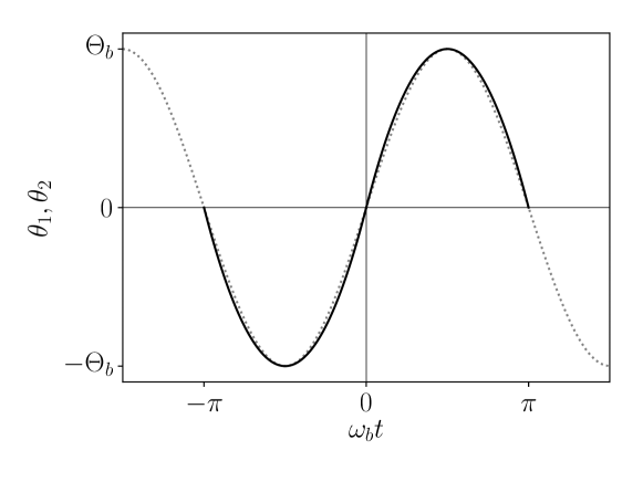
Figure 6: The rotational displacement of the support disks (dotted line) and the piecewise-parabolic approximation to the motion (solid line.)

Consider, first, the case where the centers of the support disks are fixed, and they rotate periodically in phase. The upper disk is allowed to translate and rotate. The angular excursions of the support disks are given by the equation

$$\theta_{1}=\theta_{2}=\Theta_{b}\sin(\omega_{b}t),$$ (22)

where $\theta_{1}$ is the angle of support 1, $\theta_{2}$ is the angle of support 2, $\Theta_{b}$ is the amplitude of angular oscillations, and $\omega_{b}$ is the angular frequency. The period of the oscillations is $T=2\pi/\omega_{b}$. In order to simplify calculations, equation (22) can be piecewise approximated by parabolas, as shown in Figure 6. The fitted parabolas are required to match the minimum and maximum of the sine function, as well as the crossings at the $t$-axis. In the interval from $-T/2$ to $T/2$, equation (22) is, then, approximated by the parabolas

$$\theta_{1}=\cases{\frac{4\Theta_{b}\omega_{b}^{2}}{\pi^{2}}t^{2}+\frac{4\Theta_{b}\omega_{b}}{\pi}t&for $-\pi<\omega_{b}t<0$\\ \frac{-4\Theta_{b}\omega_{b}^{2}}{\pi^{2}}t^{2}+\frac{4\Theta_{b}\omega_{b}}{\pi}t&for $0<\omega_{b}t<\pi$.}$$ (23)

The velocity at the contact point can be found by differentiating equation (23),

$$v_{1}=-R\frac{d\theta_{1}}{dt}=\cases{-\frac{8R\Theta_{b}\omega_{b}^{2}}{\pi^{2}}t-\frac{4R\Theta_{b}\omega_{b}}{\pi}&for $-\pi<\omega_{b}t<0$\\ \frac{8R\Theta_{b}\omega_{b}^{2}}{\pi^{2}}t-\frac{4R\Theta_{b}\omega_{b}}{\pi}&for $0<\omega_{b}t<\pi$,}$$ (24)

where $R$ is the disk radius. Equation (24) describes a triangle wave. This particular approximation was chosen because it allows for an easy analytic solution for the velocity of the upper disk.

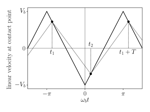
Figure 7: The velocity of the support disks (black) and the upper disk (grey) as they evolve in time.

For supports rotating in phase, contacts can never slide in opposite directions. This immediately excludes the possibility of reaching sliding configurations $S^{+-}$ and $S^{-+}$, thus $T^{+-}$ and $T^{-+}$ are set to zero accordingly. Notice that this is an important difference with the case of randomly vibrating supports, and shows that the times $T^{\pm\pm}$ depend strongly on the nature of the vibration.

Regardless of the initial condition, the system always reaches a periodic steady state, that has the same period as that of the driving. Figure 7 shows the typical stationary-state behavior of the velocities for all disks during a period of oscillation $T$. The times labeled as $t_{1}$ and $t_{2}$ are those at which the velocity of the upper disk equals the velocity of the supports, identified by the intersection of the black (supports velocity) and gray lines (velocity of the upper disk). Under the assumption of permanent sliding, these crossing points mark the transitions between the two allowed sliding configurations. When the velocities of the upper disk and the supports become equal, the relative tangential motion reverses, and a transition takes place.

Before $t_{1}$, the supports move faster than the upper disk and rotate ahead of it. Tangential forces are positive, and the sliding configuration is $S^{++}$. After $t_{1}$, and up to $t_{2}$, the supports move slower than the upper disk, thus making the tangential forces negative. The corresponding sliding configuration is $S^{--}$ in this case. At $t_{2}$, the sliding reverses again, and the configuration transitions back to $S^{++}$. At $t_{1}+T$, a cycle is completed and the systems returns to the same state as at $t_{1}$.

While at configuration $S^{--}$, between $t_{1}$ and $t_{2}$, there exists a torque that acts on the uppers disk. This torque is assumed constant and equal to $\mathcal{T}^{--}_{eq}$, given by (16). Configuration $S^{--}$ lasts during a total time $T^{--}=t_{2}-t_{1}$, at the end of which the velocity of the upper disk has suffered a net change of $R\mathcal{T}^{--}T^{--}/I$, where $I$ is the moment of inertia. Since at $t_{1}$ and $t_{2}$ the velocities of the support and the upper disk must match, the velocity at both transition points is related by the equation

$$v_{1}(t_{1})+R\mathcal{T}^{--}T^{--}/I=v_{1}(t_{2}),$$ (25)

where $v(t)$ is the function defined in equation (24). Equation (25) states that the velocity of the upper disk at $t_{1}$, given by $v_{1}(t_{1})$, plus the net change in velocity, must match the velocity of the supports at $t_{2}$, given by $v_{1}(t_{2})$. Equations of this type are referred here to as velocity-matching equations.

From $t_{2}$, and up to $t_{1}+T$, the system is at configuration $S^{++}$. The net velocity change suffered during the interval $T^{++}=t_{1}+T-t_{2}$ is given by $R\mathcal{T}^{++}T^{++}/I$, where $\mathcal{T}^{++}$ is the constant torque (given by equation (15)) and $I$ is again the moment of inertia. The velocity-matching equation between times $t_{2}$ and $t_{1}+T$ is

$$v_{1}(t_{2})+R\mathcal{T}^{++}T^{++}/I=v_{1}(t_{1}+T)=v_{1}(t_{1}),$$ (26)

where the last equality comes from the periodicity of the motion.

Solving equations (25) and (26), for $t_{1}$ and $t_{2}$, yields

$$t_{1}=\frac{\pi\mathcal{T}^{++}(\pi^{2}\mathcal{T}^{--}-4mR^{2}\Theta_{b}\omega_{b}^{2})}{4mR^{2}\Theta_{b}(\mathcal{T}^{++}-\mathcal{T}^{--})\omega_{b}^{3}}$$ (27)

$$t_{2}=\frac{\pi\mathcal{T}^{++}(\pi^{2}\mathcal{T}^{--}+4mR^{2}\Theta_{b}\omega_{b}^{2})}{4mR^{2}\Theta_{b}(\mathcal{T}^{++}-\mathcal{T}^{--})\omega_{b}^{3}}.$$ (28)

From which $T^{++}$ and $T^{--}$ can be calculated as

$$T^{++}=t_{1}+T-t_{2}=-\frac{\mathcal{T}^{--}}{\mathcal{T}^{++}-\mathcal{T}^{--}}T$$ (29)

$$T^{--}=t_{2}-t_{1}=\frac{\mathcal{T}^{++}}{\mathcal{T}^{++}-\mathcal{T}^{--}}T.$$ (30)

With $t_{1}$ and $t_{2}$ given by equations (27) and (28), and under the assumption of constant torques, the instantaneous rotational velocity of the upper disk can be written as

$${\Omega}(t)=\cases{\frac{v_{1}(t_{1})}{R}+\frac{\mathcal{T}^{--}(t-t_{1})}{I}&for $t_{1}<t<t_{2}$\\ \frac{v_{1}(t_{2})}{R}+\frac{\mathcal{T}^{++}(t-t_{2})}{I}&for $t_{2}<t<t_{1}+T$.}$$ (31)

Equation (31) yields the correct transition values ${\Omega}(t_{1})=v_{1}(t_{1})/R$ and ${\Omega}(t_{2})=v_{1}(t_{2})/R$. The mean rotational velocity of the upper disk is found by integrating equation (31) over a complete period,

$${\bar{\Omega}}=\frac{1}{T}\int_{t_{1}}^{t_{1}+T}{\Omega}(t)dt=\frac{4\Theta_{b}\omega_{b}}{\pi}\frac{\mathcal{T}^{++}+\mathcal{T}^{--}}{\mathcal{T}^{++}-\mathcal{T}^{--}}.$$ (32)

Integrating, and using equations (15) and (16), results in

$${\bar{\Omega}}=\frac{4\mu\Theta_{b}\omega_{b}\tan\theta_{T}}{\pi}.$$ (33)

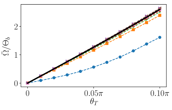
Figure 8: The rotational velocity of the upper disk ${\bar{\Omega}}$, normalized by the oscillation amplitude of the supports $\Theta_{b}$, versus the system tilt $\theta_{T}$. Numerical simulations, with the supports rotating completely in phase are show (dashed lines) for different values of the oscillating amplitude $\Theta_{b}$: $\Theta_{b}=1{\times}{10^{{-3}}}1$ (circles), $\Theta_{b}=4{\times}{10^{{-3}}}$ (squares), $\Theta_{b}=7{\times}{10^{{-3}}}$ (pluses), $\Theta_{b}=1{\times}{10^{{-2}}}$ (stars), $\Theta_{b}=4{\times}{10^{{-2}}}$ (triangles pointing right), $\Theta_{b}=7{\times}{10^{{-2}}}$ (triangles pointing left), and $\Theta_{b}=1{\times}{10^{{-1}}}$ (triangles pointing down). The agreement between simulations and the predicted velocity given by equations (33) (solid line) is excellent.

Figure 8 shows a comparison between the velocity predicted by equation (32) and results obtained from numerical simulations under the appropriate excitation conditions. Velocities obtained from numerical simulations approach the value predicted by equation (32) as the amplitude of excitation $\Theta_{b}$ increases. The agreement for large $\Theta_{b}$ becomes better since the assumption of permanent sliding is valid for large excitation intensities. For low amplitudes, the contacts spend non-negligible times in the elastic phase, and the approximation of constant sliding breaks down.

Notice that the rotational velocity in the case of synchronous rotation of the supports is always positive, and, thus, opposite in sign to case of random vibration presented in Section 3. It is possible to apply the same small-tilt analysis used to predict the sign of the velocity under random vibration to the present case of in-phase rotation of the supports. As mentioned before, for supports rotating in phase, sliding configurations $S^{+-}$ and $S^{-+}$ are inaccessible to the system. The instantaneous mean torque starting from zero tilt and slightly tilting the system is now calculated as

$$\bar{\mathcal{T}}^{*}=\frac{\mathcal{T}^{++}+\mathcal{T}^{--}}{2}=\frac{mgR\mu\sin\theta_{T}}{(1+\mu^{2})\cos\theta_{h}},$$ (34)

which, for the values of the parameters employed in the simulations, is now positive. Upon tilting the system, a positive torque acts on the upper disk, increasing its mean rotational velocity, until times $T^{++}$ and $T^{--}$ adjust, and the dynamical behavior becomes periodic. The values of $T^{++}$ and $T^{--}$ in the periodic stationary state are given by equations (29) and (30). It is easy to verify that these values comply with condition (20), and make the mean torque on the upper disk zero.

A geometric interpretation of how the system converges to periodic behavior can be given by analyzing Fig. 7. Let us assume that the system starts in a state where $T^{++}=T^{--}$, but $\theta_{T}\neq 0$. The torque on the upper disk is given by equation (34), and is positive. When ${\bar{\Omega}}$ grows under the effect of the torque, the lines describing the velocity of the upper disk in Figure 7 will shift up. This upward shift moves the points ($t_{1}$, ${\Omega}_{1}(t_{1})$) and ($t_{2}$, ${\Omega}_{2}(t_{2})$) towards the maximum of the triangle wave. This decreases the time interval $T^{++}$, while simultaneously increasing $T^{--}$, effectively decreasing the total torque on the upper disk. The process will continue until $T^{++}$ and $T^{--}$ reach their stationary values, at which the mean torque over a period vanishes.

4.2 Asynchronous rotation of the supports

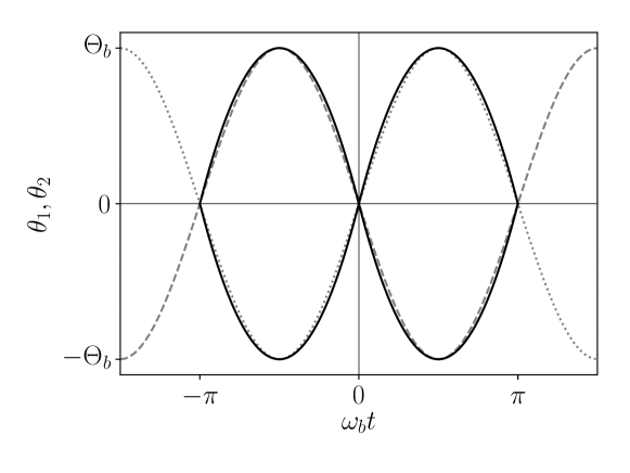
Figure 9: The rotational displacement of the support disks (dotted lines) and the piecewise-parabolic approximations to the motion (solid line.)

The same calculations used in Section 4.1 can be employed in the case of support disks rotating completely out of phase. Now the supports rotate in opposite directions, i.e., $\theta_{2}=-\theta_{1}$, and their angular velocities are also opposite in sign, $v_{2}=-v_{1}$. In the piece-wise parabolic approximation, $\theta_{1}$ and $v_{1}$ are still given by equations (23) and (24), respectively. This case is illustrated in Figure 9, where the angles of both supports are shown, together with the corresponding piece-wise parabolic approximation for their sinusoidal motion.

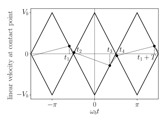
Figure 10: The velocity of the support disks (black) and the velocity of the upper disk (gray) as they evolve in time.

Figure 10 shows the velocities of the supports and the velocity of the upper disk in a cycle of period $T$, once the periodic state has been reached. Since the supports are not in phase, configurations $S^{+-}$ and $S^{-+}$ are now reachable by the system. Referring to Figure 10, and starting at $t_{1}$, the angular velocity of the upper disk is larger than that of both supports. Tangential forces are then negative, and the system is at configuration $S^{--}$. At $t_{2}$, the velocity of the upper disk becomes equal to that of support 2. The tangential force of contact 1 remains negative, but the sliding direction at contact 2 reverses, and the system transitions into configuration $S^{-+}$. At $t_{3}$, the velocity of the upper disk equals the velocity of support disk 1, reversing the sliding at contact 1, making both tangential forces positive. The system then transitions onto configuration $S^{++}$. At $t_{4}$, the velocity of the upper disk equals that of support 2 again, making tangential force at contact 2 negative, while tangential force at contact 1 remains positive. The system then transitions onto configuration $S^{+-}$. At $t_{1}+T$, the cycle ends and the system returns to configuration $S^{--}$. The velocity-matching equations introduced in Section 4.1 now take the form

$$v_{1}(t_{1})+R\mathcal{T}^{--}T^{--}/I=v_{2}(t_{2})$$ (35)

$$v_{2}(t_{2})+R\mathcal{T}^{-+}T^{-+}/I=v_{1}(t_{3})$$ (36)

$$v_{1}(t_{3})+R\mathcal{T}^{++}T^{++}/I=v_{2}(t_{4})$$ (37)

$$v_{2}(t_{4})+R\mathcal{T}^{+-}T^{+-}/I=v_{1}(t_{1}+T)=v_{1}(t_{1}),$$ (38)

where $T^{--}=t_{2}-t_{1}$, $T^{-+}=t_{3}-t_{2}$, $T^{++}=t_{4}-t_{3}$, and $T^{+-}=t_{1}+T-t_{4}$. The velocity $v_{2}$ is obtained from the condition $v_{2}=-v_{1}$, with $v_{1}$ given by equation (24).

The angular velocity of the upper disk is a piece-wise continuous function with four continuous intervals, and can be written as

$${\Omega}(t)=\cases{\frac{v_{1}(t_{1})}{R}+\frac{\mathcal{T}^{--}(t-t_{1})}{I}&for $t_{1}<t<t_{2}$\\ \frac{v_{2}(t_{2})}{R}+\frac{\mathcal{T}^{-+}(t-t_{2})}{I}&for $t_{2}<t<t_{3}$\\ \frac{v_{1}(t_{3})}{R}+\frac{\mathcal{T}^{++}(t-t_{3})}{I}&for $t_{3}<t<t_{4}$\\ \frac{v_{2}(t_{4})}{R}+\frac{\mathcal{T}^{+-}(t-t_{4})}{I}&for $t_{4}<t<t_{1}+T$.}$$ (39)

The torques acting during each sliding configuration are given by equations (15) through  (21), and are assumed constant, under the approximation of permanent sliding.

Following the same process discussed in Section 4.1, the transition times $t_{1}$ through $t_{4}$ can be obtained by solving equations (35) through (38). Using these solutions together with equation (39) for ${\Omega}$, the integral (32) can be done to obtain an expression for ${\bar{\Omega}}$. After integrating and expanding to first order in $\theta_{T}$, the approximate mean rotational velocity takes the form

$${\Omega}\approx\frac{8\mu\left(\mu^{2}+1\right)\Theta_{b}\theta_{T}\cos^{2}\left(\theta_{h}\right)}{\left(\mu^{2}+1\right)\cos\left(2\theta_{h}\right)+\mu^{2}-1}.$$ (40)

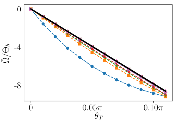
Figure 11: The rotational velocity of the upper disk ${\bar{\Omega}}$, normalized by the oscillation amplitude of the supports $\Theta_{b}$, versus the system tilt $\theta_{T}$. Numerical simulations, with the supports rotating completely out of phase, are show (dashed lines) for different values of the oscillating amplitude $\Theta_{b}$: $\Theta_{b}=1{\times}{10^{{-3}}}$ (circles), $\Theta_{b}=4{\times}{10^{{-3}}}$ (squares), $\Theta_{b}=7{\times}{10^{{-3}}}$ (pluses), $\Theta_{b}=1{\times}{10^{{-2}}}$ (stars), $\Theta_{b}=4{\times}{10^{{-2}}}$ (triangles pointing right), $\Theta_{b}=7{\times}{10^{{-2}}}$ (triangles pointing left), and $\Theta_{b}=1{\times}{10^{{-1}}}$ (triangles pointing down). The agreement between simulations and the predicted velocity given by equations (40) (solid line) is excellent.

Figure 11 shows a comparison between the velocity predicted by equation (40) and results obtained from numerical simulations. Velocities obtained from numerical simulations approach the value predicted by equation (40) as $\Theta_{b}$ increases and the permanent-sliding approximation becomes increasingly accurate. The agreement for large amplitudes $\Theta_{b}$ is, again, excellent.

Contrary to the case discussed in Section 4.1, when the supports rotate out of phase the rotational velocity is always negative. For this reason, out-of-phase excitation resembles the case of random vibration presented in Section 3. In both the random and the out of phase cases, the system can access all four sliding configurations $S^{\pm\pm}$. The analysis to predict the sign of the velocity, based on equation (21), is the same for both cases, and predicts a negative velocity in both of them.

5 Conclusion

In this work, a new rotational ratcheting mechanism was reported, which occurs in a simple packing consisting of a single disk supported against gravity by other two. It was shown, using numerical simulations that, if the supports are vibrated and the system is tilted, the upper disk acquires a non-zero mean rotational velocity, even though the vibration is completely left-right symmetric. It was also shown that the details of the vibration are important, as changing them may lead to velocity inversion of the upper disk.

Similarly to the case of the elasto-plastic oscillator (EPO), for rotation to appear, friction forces must be asymmetric for different directions of sliding. This asymmetry originates in the correlation between contact forces and the direction at which contacts slide. The notion of translational equilibrium points (TEP) was introduced to explain the origin of these correlations. The TEPs define translational equilibrium points towards which the system converges during sliding. Since each of the two contacts can slide in two directions, there exist four different sliding configurations, each one with a different TEP. In this sense, the 3-disk system may be regarded as a generalization of the EPO, with four possible sliding configurations instead of two.

One might attempt to apply to this 3-disk system, some of the approaches that have been previously used to analyze the EPO under random loading (see for example [43, 50, 49]). These techniques, however, assume rare visits to the plastic domain, a limit case completely opposite to the one elaborated upon in this work. Rotation in the 3-disk system requires contacts to be saturated (sliding) a sizeable fraction of the time, since it is only during sliding that correlations among forces appear, and the system evolves towards the TEP. This makes such mentioned techniques hard to adapt to the conditions of vibration described here.

Here, two simple deterministic cases were solved under the assumption of constant sliding. More work is required to obtain an expression for the rotational velocity with supports that are vibrated randomly. This case will be addressed in future work.

As a final note, we have recently observed a related phenomena of self-organized rotations in disk packings (manuscript in preparation). We found that when two-dimensional disk packings are vibrated from the bottom, each of the disks within the packing acquires a rotational velocity that depends on the local configuration of contacts of each disk. Given that the contact network of a packing is essentially random, rotations in such packings are an example of noise rectification in disordered systems. Since large packings are generalizations of the simple packing presented here, one can expect that some of the mechanisms described in this work remain at play for packings of more than three disks.

References

References

- [1] Feynman R P, Leighton R B and Sands M 2011 The Feynman Lectures on Physics vol 1 (Basic books)
- [2] Astumian R D and Bier M 1994 Physical Review Letters 72 1766–1769
- [3] Reimann P 2002 Physics Reports 361 57–265 ISSN 0370-1573
- [4] Astumian R D and Hänggi P 2002 Physics Today 55 33–39 ISSN 0031-9228, 1945-0699
- [5] Hänggi P, Marchesoni F and Nori F 2005 Annalen der Physik 14 51–70 ISSN 1521-3889
- [6] Hänggi P and Marchesoni F 2009 Reviews of Modern Physics 81 387–442
- [7] Reimann P and Hänggi P 2014 Applied Physics A 75 169–178 ISSN 0947-8396, 1432-0630
- [8] Parrondo J M R and Cisneros B J d 2014 Applied Physics A 75 179–191 ISSN 0947-8396, 1432-0630
- [9] Costantini G, Marini Bettolo Marconi U and Puglisi A 2007 Physical Review E 75 061124
- [10] Cleuren B and Broeck C V d 2007 Europhysics Letters (EPL) 77 50003 ISSN 0295-5075
- [11] Van den Broeck C, Kawai R and Meurs P 2004 Physical Review Letters 93 090601
- [12] Eshuis P, van der Weele K, Lohse D and van der Meer D 2010 Physical Review Letters 104 248001
- [13] Gnoli A, Petri A, Dalton F, Pontuale G, Gradenigo G, Sarracino A and Puglisi A 2013 Physical Review Letters 110 120601
- [14] Leff H S and Rex A F (eds) 2014 Maxwell’s Demon: Entropy, Information, Computing (Princeton University Press) ISBN 978-0-691-60546-3
- [15] Nordén B, Zolotaryuk Y, Christiansen P L and Zolotaryuk A V 2001 Physical Review E 65 011110
- [16] Altshuler E, Pastor J M, Garcimartín A, Zuriguel I and Maza D 2013 PLOS ONE 8 e67838 ISSN 1932-6203
- [17] Peraza-Mues G, Carvente O and Moukarzel C F 2017 International Journal of Modern Physics C 28 1750021
- [18] Gear C W 1971 Communications of the ACM 14 176–179
- [19] Cundall P A and Strack O D L 1979 Géotechnique 29 47–65 ISSN 0016-8505
- [20] Shäfer J, Dippel S and Wolf D E 1996 Journal de Physique I 6 16
- [21] Di Renzo A and Di Maio F P 2004 Chemical Engineering Science 59 525–541 ISSN 0009-2509
- [22] Kruggel-Emden H, Simsek E, Rickelt S, Wirtz S and Scherer V 2007 Powder Technology 171 157–173 ISSN 0032-5910
- [23] Kruggel-Emden H, Wirtz S and Scherer V 2008 Chemical Engineering Science 63 1523–1541 ISSN 0009-2509
- [24] Kruggel-Emden H, Wirtz S and Scherer V 2009 Journal of Pressure Vessel Technology 131 024001
- [25] Silbert L E, Ertaş D, Grest G S, Halsey T C and Levine D 2002 Physical Review E 65 031304
- [26] McNamara S, García-Rojo R and Herrmann H J 2008 Physical Review E 77 031304
- [27] Chandrasekhar S 1943 Reviews of Modern Physics 15 1–89
- [28] Caughey T K 1960 Journal of Applied Mechanics 27 640–643 ISSN 0021-8936
- [29] Jennings P C 1964 Journal of the Engineering Mechanics Division 90 131–166
- [30] Iwan W D 1965 Journal of Applied Mechanics 32 921–925 ISSN 0021-8936
- [31] Masri S F 1975 The Journal of the Acoustical Society of America 57 106–112 ISSN 0001-4966
- [32] Miller Gregory R and Butler Mark E 1988 Journal of Engineering Mechanics 114 536–550
- [33] Capecchi D and Vestroni F 1990 International Journal of Non-Linear Mechanics 25 309–317 ISSN 0020-7462
- [34] Capecchi D 1991 Dynamics and Stability of Systems 6 89–106 ISSN 0268-1110
- [35] Capecchi D 1993 International Journal of Solids and Structures 30 3303–3314 ISSN 0020-7683
- [36] Chatterjee S, Mallik A K and Ghosh A 1996 Journal of Sound and Vibration 191 129–144 ISSN 0022-460X
- [37] Liu C S and Huang Z M 2004 Journal of Sound and Vibration 273 149–173 ISSN 0022-460X
- [38] Ahn Il-Sang, Chen Stuart S and Dargush Gary F 2006 Journal of Engineering Mechanics 132 411–421
- [39] Csernák G and Stépán G 2006 Journal of Sound and Vibration 295 649–658 ISSN 0022-460X
- [40] Challamel N and Gilles G 2007 Journal of Sound and Vibration 301 608–634 ISSN 0022-460X
- [41] Challamel N, Lanos C, Hammouda A and Redjel B 2007 Physical Review E 75 026204
- [42] Caughey T K 1960 Journal of Applied Mechanics 27 649–652 ISSN 0021-8936
- [43] Karnopp D and Scharton T D 1966 The Journal of the Acoustical Society of America 39 1154–1161 ISSN 0001-4966
- [44] Iwan W D and Lutes L D 1968 The Journal of the Acoustical Society of America 43 545–552 ISSN 0001-4966
- [45] Vanmarcke E H and Veneziano D 1973 Probabilistic seismic response of simple inelastic systems Proceedings of the fifth world conference on earthquake engineering vol 2 pp 2851–863
- [46] Lutes L D and Takemiya H 1974 Journal of the Engineering Mechanics Division 100 343–358
- [47] Grossmayer R L 1979 Journal of Sound and Vibration 65 353–379 ISSN 0022-460X
- [48] Wen Y K 1980 Journal of Applied Mechanics 47 150–154 ISSN 0021-8936
- [49] Ditlevsen O and Bognár L 1993 Probabilistic Engineering Mechanics 8 209–231 ISSN 0266-8920
- [50] Bouc R and Boussaa D 1998 Comptes Rendus de l’Académie des Sciences - Series IIB - Mechanics-Physics-Astronomy 326 475–482 ISSN 1287-4620
- [51] Bouc R and Boussaa D 2002 International Journal of Non-Linear Mechanics 37 1397–1406 ISSN 0020-7462
- [52] Feau C 2008 Probabilistic Engineering Mechanics 23 36–44 ISSN 0266-8920
- [53] McNamara S, García-Rojo R and Herrmann H 2005 Physical Review E 72 021304