Analyzing the Trade-offs in Using Millimeter Wave Directional Links for High Data Rate Tactile Internet Applications

Abstract

Ultra-low latency and high reliability communications are the two defining characteristics of Tactile Internet (TI). Nevertheless, some TI applications would also require high data-rate transfer of audio-visual information to complement the haptic data. Using Millimeter wave (mmWave) communications is an attractive choice for high datarate TI applications due to the availability of large bandwidth in the mmWave bands. Moreover, mmWave radio access is also advantageous to attain the air-interface-diversity required for high reliability in TI systems as mmWave signal propagation significantly differs to sub-6 GHz propagation. However, the use of narrow beamwidth in mmWave systems makes them susceptible to link misalignment-induced unreliability and high access latency. In this paper, we analyze the trade-offs between high gain of narrow beamwidth antennas and corresponding susceptibility to misalignment in mmWave links. To alleviate the effects of random antenna misalignment, we propose a beamwidth-adaptation scheme that significantly stabilize the link throughput performance.

I Introduction

Tactile Internet (TI) aims to enable interaction with remote environments in perceived real-time through the delivery of haptic information over wired/wireless networks. This has led to the two main requirements for network infrastructure facilitating TI, i.e., ultra-low latency and high reliability [1]. Although haptic information may be encoded in a few bytes, there are several applications such as robotic surgery, autonomous driving, where transfer of high quality audio-visual information would be quintessential to complement the haptic information [2]. This would add another requirement for TI, i.e., sustained high data-rate communication links. Consequently, such applications would require wireless interfaces that are highly-reliable, can provide ultra-low latency, and are also able to sustain high data rates in order of Multi-Gbps.

To achieve the carrier-grade reliability over wireless links, potential solutions include frequency diversity using multiple uncorrelated links and spatial diversity using simultaneous connectivity to multiple spatially-uncorrelated base stations[3]. These approaches are also referred as interface-diversity techniques [4]. To achieve the latency requirements at link-layer, short packet length is proposed to reduce the total transmission interval instead of transmitting long packets [5, 6].

In the context of fifth-generation (5G) networks, millimeter Wave (mmWave) frequency band (30 GHz to 300 GHz) has emerged as a promising candidate for multi-Gbps wireless connectivity due to availability of large bandwidth chunks in mmWave frequency band [7, 8]. Since radio-interface diversity is important from reliability perspective, using mmWave radio-interfaces would certainly benefit the TI applications as mmWave signals propagation is highly likely to be uncorrelated to sub-6 GHz signal propagation due to its differing propagation characteristics. In this context we envision a hybrid radio access architecture to support TI applications where sub-6 GHz access will be used for transmitting haptic information while mmWave access will be used for high data-rate transmission of audio-visual information. However, using mmWave communications for TI application is not straight-forward. Specifically, the use of narrow beamwidth directional antennas, which is necessary to combat high-pathloss at mmWave frequencies [9], can result in frequent link outages due to antenna misalignment [10]. Thus providing a sustained high data-rate radio interface for TI applications at mmWave frequencies is not a straight-forward task.

Ideally, a narrow beamwidth antenna should always result in better signal quality compared to a broader beamwidth antenna as antenna gain and beamwidth are reciprocal to each other. However, in practical situations, following two factors have a significant impact on the performance of a narrow beamwidth directional link:
(i) Beam misalignment – the alignment of Tx and Rx antennas can be disturbed by many factors such as device holding pattern, random user movements, orientation error and vibrations that would result in unstable link quality. Since link availability is one of the most important indicator of link reliability [11], it is highly important to analyze the impact of beam alignment on link quality for different transmitter and receiver beamwidths. This is specifically interesting for TI applications where link outages are not at all desired.
(ii) Beam setup time– finding best Tx and Rx antenna directions is essential to establish a mmWave link. mmWave standards IEEE 802.15.3c [12]) and (IEEE 802.11ad [13] have proposed beamforming-protocols to find the Tx and Rx beams that result in best signal quality. The beam-search space is inversely proportional to the beamwidths of Tx and Rx antennas. In the case of narrow beamwidths, a significant fraction of allocated time-slot can be exhausted finding the best Tx/Rx beams. Hence the beam-searching can be a considerable overhead in narrow-beamwidth mmWave links.

Thus the use of directional antennas at mmWave frequencies impacts both the reliability and latency performance which are of paramount importance to TI applications. Further, the TI applications do involve movement, at least within a constrained domain, thus proper beam forming and alignment is a must. It is important to ensure that the random misalignment does not impact the link performance; and when link disruption is unavoidable, beam setup procedure should be fast enough to minimize the impact of outage.

The available literature on mmWave communications has mainly dealt with capacity analysis or beamforming design. There are very few papers that consider mmWave communications for ultra low latency and high reliability communication (URLLC) scenarios [14, 15, 16, 17, 18]. In [14], various challenges of achieving URLLC at mmWave band are highlighted. It is argued that a significant reworking of the entire protocol stack (short frame size at physical layer, dynamic MAC protocols, moving content closer to edge, etc.) is required if mmWave radio access is used for URLLC. In [15], it is shown that cooperative networking can significantly improve the latency performance of mmWave based heterogeneous networks. In [16], two strategies, namely, traffic dispersion and networking densification are proposed to reduce the end to end in mmWave wireless networks. Here dispersion stands for offloading traffic to different spatial paths using distributed antenna systems while densification refers to increasing the density of mmWave BSs. It is shown that both the strategies improve latency performance for a given sum budget power. In [17], the problem of reliability and latency in mmWave massive multiple-input multiple-output (MIMO) networks is studied by using the Lyapunov technique that follows utility-delay control approach and successfully adapts to channel variations and the queue dynamics. In [18], the feasibility of using mmWave access for URLLC considering dynamic blockages is considered. It is shown that the optimal BS deployment is driven by reliability and latency constraints instead of coverage and rate requirements.

All the above papers follow a system level modeling approach and do not account for the impact of beamwidth on performance of individual links considering medium access control (MAC) overheads amounting to use of directional antennas. In [19, 20], the performance evaluations of contention access in IEEE 802.11ad MAC protocol is done assuming coarse-sector beamwidths and without considering alignment and searching overheads. There are few papers that separately consider the beam searching overhead [21, 22, 23] or the misalignment [24, 25, 26]. In [21], an efficient beam switching mechanism is proposed that utilizes a modified Rosenbrock numerical algorithm to select the best beam-pair. Using the direction estimates at 2.4 and 5 GHz, it is possible to infer the coarse beam directions of 60 GHz links [22]. Since direction estimates at 2.4/5 GHz is obtained using passively-heard frames, it enormously reduces the searching overheads. In [27], it is shown that the exhaustive search outperforms hierarchal search in terms of asymptotic misalignment probability. In [23], capacity of 60 GHz link is analysed considering beam-searching overhead while using an ideal flat-top antenna model. This paper does not take into account the impact of antenna misalignment. Moreover, the flat-top antenna model assumed in this paper transforms the continuously varying antenna gains into binary values that are not suitable for analysing the impact of misalignment. Our work is close to this paper, however we consider a Gaussian antenna model and include misalignment errors as well into our link modeling framework. In [25], it is numerically demonstrated that the Gaussian main-lobe antenna pattern, which we have adopted in this paper, can represent the mmWave directional antennas with a reasonable accuracy.The rate analysis of mmWave mobile network using stochastic geometry is presented in [24]. However, beam set up overhead is ignored and mainly employ flat-top antenna models thus unable to provide accurate impact of misalignment. In [26], authors also use stochastic geometry framework and employ Sinc and Cosine antenna patterns at BSs to evaluate the impact of misalignment. However, beam-searching overhead is not considered.

In summary, despite the plethora of recent literature on mmWave communications, there is no prior work that has holistically considered the consequential trade-offs of using narrow beamwidths, i.e., increase in antenna gains at the cost of highly un-sustained link quality that is bound to increase the susceptibility to link unreliability and high-latency. In this paper we aim to fill this gap. Our main contributions are as follows.

• We develop a novel link capacity optimization framework that shows the existence of optimum TX/Rx beamwidths. Our model jointly considers the beam-misalignment, beam-searching overhead and allocated time-slot length to model the capacity of mmWave links.

• We show that although the narrow beams result in high throughput links, the resulting links are highly susceptible to beam-misalignment. Such links are highly un-reliable and are not suitable to support the TI applications.

• We propose a beamwidth-adaptation scheme that is misalignment-aware and significantly stabilizes the quality of mmWave links and result in (50% to 150%) improvement in average link capacity.

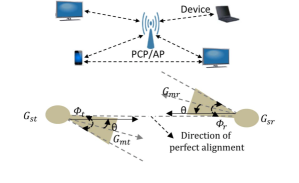
(a) Network architecture.

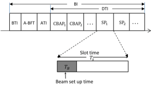
(b) Beacon Interval.

Figure 1: IEEE 802.11ad network architecture and beacon interval.

II Preliminaries of IEEE 802.11ad

Fig. 1(a) shows an IEEE 802.11ad Personal Basic Service Set (PBSS) formed by the 60 GHz stations (STAs) where one of them acts as PBSS Control Point/Access Point (PCP/AP). IEEE 802.11ad employs a hybrid medium access control protocol consisting of both contention-based channel access (CSMA/CA) and fixed TDMA based channel access. Fig. 1(b) shows the timings in an IEEE 802.11ad MAC that are based on beacon intervals (BI) which consists of: (i) beacon transmission interval (BTI); (ii) association beamforming training (A-BFT) where STAs associate with the PCP/AP; (iii) announcement time interval (ATI) where the exchange of management information between PCP/AP and the STAs happens; and (iv) data transfer interval (DTI), which consists of contention-based access periods (CBAPs) and fixed-access service periods (SPs). CBAPs use CSMA/CA based channel access mechanism while during SPs, TDMA access mechanism is used. In this paper, we mainly focus on the SPs part of the BI where high speed data transmission using narrow beamwidth happens.

II-A Antenna model

To examine the effect of beam alignment errors on the communication link performance, detailed mathematical models of antennas are needed. Generally, capturing all essential characteristics of the real-world antennas in a simple analytical expressions/model is difficult. The most widely used cone-plus-circle antenna model [23] assumes constant gains for both the main and the side lobes. The assumption of constant gain for main lobe makes it unsuitable for examining the effect of misalignment. In this case, any alignment error smaller than the beamwidth of main lobe would be unnoticed. We use a relatively pragmatic antenna model employing the Gaussian main lobe radiation pattern, which is proposed in IEEE 802.15.3c [12]. Let $G_{m}^{\phi}(\theta)$ and $G_{s}^{\phi}$ represent the mainlobe and sidelobe gains, respectively. The analytical model is represented by,

$$G^{\phi}(\theta)=\begin{cases}\begin{array}[]{ll}G_{m}^{\phi}(\theta)=\left(\frac{1.6162}{\sin(\frac{\phi}{2})}\right)^{2}e^{-K_{1}{4\log_{e}(2)}\left(\frac{\theta}{\phi}\right)^{2}},&|\theta|\leq 1.3\phi,\\ G_{s}^{\phi}=e^{-2.437}\phi^{-0.094},&|\theta|>1.3\phi.\end{array}\end{cases}$$ (1)

Where, $\phi$ is the half power beamwidth (HPBW) beamwidth and $\theta$ is the deviation angle of antenna boresight from axis of perfect alignment. The main lobe beamwidth $\phi_{ML}$ (defined as frequency intervals between -20 dB gain levels relative to the peak gain) is approximately $\phi_{ML}=2.6\phi$.

\psfrag{x}[cc][cc][0.75]{\small{Misalignment, $\theta$\textdegree}}\psfrag{y}[cc][cc][0.75]{\small{Gain (dB)}}\includegraphics[width=117.07924pt]{GainMisalignment_2018.eps}

Figure 2: Gain vs beam misalignment.

The the main lobe gain with varying alignment error for different HPBW $\phi$ is shown in Fig. 2. We can observe that the gain curve of smaller beamwidth decays faster than the wider beamwidth. This implies that the narrow beam (high gain) antennas are most affected by the alignment errors. Consequently, in presence of alignment errors, the effective gains of Tx and Rx would be way less than the expected gains. Using the Gaussian main lobe offers different gains for different value of alignment errors as opposed to the ideal cone-plus-circle antenna model where antenna gain has binary values, thus making it possible to track the impact of alignment errors on the link quality.

It should be noted that if maximum possible misalignment, denoted as $|\theta_{max}|$, is greater than the half of main lobe beamwidth, antenna pointing error of main lobe would lead to link failure as antennas would no longer be able to communicate using the main lobe. Therefore, to ensure the link availability, $\frac{\phi_{ML}}{2}\geq|\theta_{max}|$ must be satisfied.

II-B Beam Training procedure

IEEE IEEE 802.11ad use a 2-level beamforming protocol. In the $1^{st}$ stage, devices pair that want to establish a connection start scanning, using wider beamwidths called quasi-omni (QO) levels or sector levels. Generally, the beamwidth of sector-level could be 180$\degree$ or 90$\degree$. Once the best Tx and Rx sectors are found, high resolution beams (1°-10°) are used in the $2^{nd}$ stage of beamforming procedure.

Fig. 3 depicts the sector and beam level beamwidths where many fine beams are contained within a coarse sector. To identify the best Tx and Rx beams, training sequences are transmitted in all the possible directions. Let the sector level Tx and Rx beamwidths are denoted by $\Omega_{t}$ and $\Omega_{r}$, respectively. Let the beam level Tx and Rx beamwidth are denoted by $\phi_{t}$ and $\phi_{r}$, respectively. Then, the total number of beam directions to be probed becomes $\frac{\Omega_{t}}{\phi_{t}}$ Tx and $\frac{\Omega_{r}}{\phi_{x}}$ Rx beams, respectively. Therefore, the total time required to search the best Tx and Rx beams (represented by $T_{B}$) can be given as,

$$T_{B}^{\phi_{t},\phi_{r}}=\left(\frac{2\pi}{\Omega_{t}}+\frac{2\pi}{\Omega_{r}}\right)T_{p}+\left(\frac{\Omega_{t}}{\phi_{t}}+\frac{\Omega_{r}}{\phi_{r}}\right)T_{p},$$ (2)

here, $T_{p}$ represents the transmission time of a beam training sequence. According to IEEE 802.11ad, the $1^{st}$ stage beamforming is performed during A-BFT period while the $2^{nd}$ stage beamforming may be performed during SP or during A-BFT. To consider the effect of beam-training overhead on the effective channel time available for data transmission, we assume that both stages of beamforming are performed during SP.

As depicted in Fig. 1(b), a slot $T_{S}$ granted to a device pair is divided into two parts: (i) $T_{B}$ which is used for beam training; and (ii) $T_{S}-T_{B}$ which is used for data transmission. This implies that the beam training time $T_{B}$ impacts the effective transmission time. From (2), we deduce that the beam training overhead $T_{B}$ is dependent on Tx/Rx beamwidths assuming a fixed $T_{p}$. As the beamwidth decreases, the beam-search space expands thus forcing a trade-off between the high antenna gains and the corresponding increase in the beam searching overhead.

\psfrag{x}[cc][cc][0.75]{\small{Beamwidth, $\phi$\textdegree}}\psfrag{y}[cc][cc][0.75]{\small{Capacity (bits/slot/Hz)}}\includegraphics[width=117.07924pt]{beamtrainingProtocol2018}

Figure 3: IEEE 802.11ad beam patterns.

III Modeling of link capacity considering beam setup time and misalignment

Let $P_{t}$ be the Tx power, $\lambda$ be the carrier wavelength, $\alpha$ be the path loss exponent, and $G_{t}$, $G_{r}$ be the Tx and Rx antenna gains, respectively. By applying the Friis’s free-space pathloss equation, the received power $P_{r}$ at a $d$ m from the Tx is $P_{r}=G_{t}G_{r}G_{0}(\lambda,d)P_{t}$. Where, $G_{0}(\lambda,d)=\left(\frac{\lambda}{4\pi d}\right)^{\alpha}$ represents the overall effect of propagation and free-space path losses if Tx and Rx are separated by $d$ m. We define $\eta_{\phi_{t},\phi_{r}}$ as the fraction of allocated time slot $T_{S}$ used for data transmission, i.e., $\eta_{\phi_{t},\phi_{r}}=\left(1-\frac{T_{B}^{\phi_{t},\phi_{r}}}{T_{s}}\right)$. Then, the achievable data rate ($r^{\phi_{t},\phi_{r}}$ (bits/slot/Hz)) for a given Tx-Rx beamwidths is given by,

$$r^{\phi_{t},\phi_{r}}(\theta_{t},\theta_{r})=\eta_{\phi_{t},\phi_{r}}\log_{2}\left(1+\frac{G^{\phi_{t}}_{t}(\theta)G^{\phi_{r}}_{r}(\theta)G_{0}(\lambda,d)P_{t}}{N_{0}W}\right).$$ (3)

Here, $N_{0}$ is the white Gaussian noise’s one-sided power spectral density, $W$ represents the signal bandwidth and Tx and Rx antenna gains $G^{\phi_{t}}_{t}(\theta)$ and $G^{\phi_{r}}_{r}(\theta)$ are given in (1). $\eta_{\phi_{t},\phi_{r}}$, as previously defined, depends on sector beamwidths $\Omega_{t}$ and $\Omega_{r}$, pencil beam beamwidths $\phi_{t}$ and $\phi_{r}$, and allocated time slot $T_{S}$. The objective is to find the optimum Tx and Rx beamwidths ($\phi_{t}$ and $\phi_{r}$) that can maximize the link capacity $r^{\phi_{t},\phi_{r}}(\theta_{t},\theta_{r})$. Here, for simplicity and without loss of generality we assume $\theta_{r}=\theta_{t}=\theta$. Therefore, the resulted optimization problem can be written as,

$$\mathbb{P}1:\quad\mathop{\max}\limits_{{\phi_{r}},{\phi_{t}}}r({\phi_{r}},{\phi_{t}},{\theta})$$

$$\hskip 42.67912pt=\eta_{{\phi_{r}},{\phi_{t}}}{\rm{log}}\left(1+{c_{1}({\phi_{r}},{\phi_{t}})}{{\rm e}^{-{{(\frac{{{\theta}}}{{{\phi_{r}}}})}^{2}}-{{(\frac{{{\theta}}}{{{\phi_{t}}}})}^{2}}}}\right)$$ (4)

$$\hskip 31.2982pts.t.\,\,|\theta|\leq\min[2.6\phi_{t},2.6\phi_{r}]$$

$$\hskip 42.67912pt\,\,\,\,\phi_{t}\leq\Omega_{t},\phi_{r}\leq\Omega_{r}$$

Here, ${\Omega_{r}},{\Omega_{t}}\in\left({0,2\pi}\right]$ and ${c_{1}}({\phi_{r}},{\phi_{t}})$ (assuming both Tx and Rx stay within their main lobes) is,

$$c_{1}({\phi_{r}},{\phi_{t}})={{{(\frac{\lambda}{{4\pi d}})}^{\alpha}}\frac{{{P_{t}}}}{{{N_{0}}W}}\left({\frac{{{{1.6161}^{4}}}}{{{{\sin}^{2}}(\frac{{{\phi_{r}}}}{2}){{\sin}^{2}}(\frac{{{\phi_{t}}}}{2})}}}\right)}$$ (5)

Since, we do not have any prior information on random variable $\theta$, we assume $\theta$ is uniformly distributed in ${\theta}\in\left[{-\theta_{m},\theta_{m}}\right]$ with pdf $f(\theta)$ given as,

$$f(\theta)=\begin{cases}\begin{array}[]{ll}\frac{1}{2\theta_{m}},&|\theta|\leq\theta_{m},\\ 0,&|\theta|>\theta_{m}.\end{array}\end{cases}$$ (6)

The optimization problem $\mathbb{P}1$ is a robust optimization problem in which a certain measure of robustness is sought with respect to the random variable $\theta$.

Lemma 1.

The objective function of the optimization problem $\mathbb{P}1$ is a concave function with respect to the variable $\theta$.

Proof.

The objective function of the problem $\mathbb{P}1$ is in the form of ${\rm log}(1+{\rm e}^{-x^{2}})$. Since, $-x^{2}$ is concave function and ${\rm e}(.)$ and ${\rm log}(.)$ are functions that preserve concavity [28], the overall function is still a concave function. ∎

Given Lemma 1, we invoke Jensen’s inequality. Therefore,

$$E_{\theta}\left[{\eta_{{\phi_{r}},{\phi_{t}}}{\rm log}\big{(}1+{c_{1}}({\phi_{r}},{\phi_{t}}){{\rm e}^{-(\frac{{{\theta^{2}}}}{{{\phi_{r}}^{2}}})-(\frac{{{\theta^{2}}}}{{{\phi_{t}}^{2}}})}}\big{)}}\right]$$

$$\hskip 28.45274pt\leq\eta_{{\phi_{r}},{\phi_{t}}}{\rm log}\big{(}1+{c_{1}}({\phi_{r}},{\phi_{t}}){{\rm e}^{-(\frac{{E[{\theta^{2}}]}}{{{\phi_{r}}^{2}}})-(\frac{{E[{\theta^{2}}]}}{{{\phi_{t}}^{2}}})}}\big{)}$$

$$\hskip 28.45274pt{\mathop{=}\limits^{\left(a\right)}}\eta_{{\phi_{r}},{\phi_{t}}}{\rm log}\big{(}1+{c_{1}}({\phi_{r}},{\phi_{t}}){{\rm e}^{-(\frac{{\frac{\theta_{m}^{2}}{3}}}{{{\phi_{r}}^{2}}})-(\frac{{\frac{\theta_{m}^{2}}{3}}}{{{\phi_{t}}^{2}}})}}\big{)}$$ (7)

where $(a)$ follows from the assumption of $\theta$ as a zero-mean uniformly distributed random variable. Therefore, the optimization problem can be rewritten as

$$\mathbb{P}2:\quad\mathop{\max}\limits_{{\phi_{r}},{\phi_{t}}}r^{{\phi_{r}},{\phi_{t}}}$$

$$\hskip 42.67912pt=\eta_{{\phi_{r}},{\phi_{t}}}{\rm{log}}\bigg{(}1+{{{{(\frac{\lambda}{{4\pi d}})}^{\alpha}}\frac{{{P_{t}}}}{{{N_{0}}W}}\bigg{(}{\frac{{{{1.6161}^{4}}}}{{{{\sin}^{2}}(\frac{{{\phi_{r}}}}{2}){{\sin}^{2}}(\frac{{{\phi_{t}}}}{2})}}}\bigg{)}}}$$

$$\hskip 42.67912pt\times{{\rm e}^{-{{(\frac{{{\theta_{m}}}}{{{3\phi_{r}}}})}^{2}}-{{(\frac{{{\theta_{m}}}}{{{3\phi_{r}}}})}^{2}}}}\bigg{)}$$ (8)

Lemma 2.

The objective function of the optimization problem $\mathbb{P}2$ is a strictly quasi-concave function of variables $\phi_{r}$ and $\phi_{t}$.

Proof.

In order to prove Lemma 2, considering the fact that the objective function is a symmetric function in $\phi_{r}$ and $\phi_{t}$, we first prove that a function of the form $\frac{{{{\rm{e}}^{-{x^{-2}}}}}}{{{{\sin}^{2}}\left({\frac{x}{2}}\right)}}$ is a strictly quasi-concave function.

Considering the theorem from [28], if $\frac{{{{\rm{e}}^{-{x^{-2}}}}}}{{{{\sin}^{2}}\left({\frac{x}{2}}\right)}}>a$ and $\frac{{{{\rm{e}}^{-{y^{-2}}}}}}{{{{\sin}^{2}}\left({\frac{y}{2}}\right)}}>a$, then,

$$f(\lambda x+(1-\lambda)y)$$

$$\hskip 28.45274pt=\frac{{{{\rm{e}}^{-{{\left({\lambda x+(1-\lambda)y}\right)}^{-2}}}}}}{{{{\sin}^{2}}\left({\frac{{\left({\lambda x+(1-\lambda)y}\right)}}{2}}\right)}}>\left\{\begin{array}[]{l}\frac{{{{\rm{e}}^{-{y^{-2}}}}}}{{{{\sin}^{2}}\left({\frac{x}{2}}\right)}}\,\,\,\,\,\,\,\,{\rm{if}}\,\,\,x\geq y\\ \frac{{{{\rm{e}}^{-{x^{-2}}}}}}{{{{\sin}^{2}}\left({\frac{y}{2}}\right)}}\,\,\,\,\,\,\,\,{\rm{if}}\,\,\,x<y\end{array}\right.$$

$$\hskip 28.45274pt>\left\{\begin{array}[]{l}\frac{{a{{\sin}^{2}}\left({\frac{y}{2}}\right)}}{{{{\sin}^{2}}\left({\frac{x}{2}}\right)}}\,\,\,\,\,\,\,\,{\rm{if}}\,\,\,x\geq y\\ \frac{{a{{\sin}^{2}}\left({\frac{x}{2}}\right)}}{{{{\sin}^{2}}\left({\frac{y}{2}}\right)}}\,\,\,\,\,\,\,\,{\rm{if}}\,\,\,x<y\end{array}>a.\right.$$ (13)

Therefore, functions of the form $\frac{{{{\rm{e}}^{-{x^{-2}}}}}}{{{{\sin}^{2}}\left({\frac{x}{2}}\right)}}$, are quasi-concave. In addition, if $f(.)$ is a strictly quasi-concave function and $g$ is an increasing function, the composite function $g(f(.))$ is a strictly quasi-concave function [28]. Therefore, given that ${\rm log}(1+x)$ is an increasing function of $x$, ${\rm log}(1+{\frac{{{{\rm{e}}^{-{x^{-2}}}}}}{{{{\sin}^{2}}\left({\frac{x}{2}}\right)}}})$ is strictly quasi-concave. Moreover, ${1-(\frac{{2\pi}}{{{\Omega_{t}}}}+\frac{{2\pi}}{{{\Omega_{r}}}})\frac{{{T_{p}}}}{{{T_{s}}}}-(\frac{{{\Omega_{t}}}}{{{x}}})\frac{{{T_{p}}}}{{{T_{s}}}}}$ is a nonnegative strictly quasi-concave function, given the typical values of its parameters $T_{p}$, $T_{s}$, $\Omega_{t}$ and $\Omega_{r}$ (Proof comes in the Appendix). Given the fact that the product of nonnegative strictly quasi-concave functions is quasi-concave [29], the overall function which is in the form of $\left({1-(\frac{{2\pi}}{{{\Omega_{t}}}}+\frac{{2\pi}}{{{\Omega_{r}}}})\frac{{{T_{p}}}}{{{T_{s}}}}-(\frac{{{\Omega_{t}}}}{{{x}}})\frac{{{T_{p}}}}{{{T_{s}}}}}\right){\rm log}(1+{\frac{{{{\rm{e}}^{-{x^{-2}}}}}}{{{{\sin}^{2}}\left({\frac{x}{2}}\right)}}})$ is also a strictly quasi-concave function. ∎

Since, the objective function in $\mathbb{P}2$ is strictly quasi-concave, the maximizer is unique [28]. Given that the objective function in (III) is a differentiable function with respect to $\phi_{r}$ and $\phi_{t}$, the maximum value is achieved by the well-known necessary and sufficient condition $\nabla r({\phi_{r}},{\phi_{t}})=0$. The derivative of the objective function with respect to $\phi_{r}$ and $\phi_{t}$ are given in (III) and (III). Therefore, we have a set of two equations of two variables. However, finding the solution of the equation $\nabla r({\phi_{r}},{\phi_{t}})=0$ is analytically complex. Therefore, in such cases the problem must be solved using iterative algorithms [28].

$$\frac{\partial}{{\partial{\phi_{r}}}} =\frac{\bigg{(}\eta_{\phi_{t},\phi_{r}}c_{1}({\phi_{t}},{\phi_{r}}){\rm e}^{-\frac{\theta^{2}_{m}}{3\phi^{2}_{r}}}\left(\frac{2\theta^{2}_{m}}{3\phi^{3}_{r}}-\cot{(\frac{{{\phi_{r}}}}{2}}\right)\bigg{)}}{\left(1+c_{1}({\phi_{t}},{\phi_{r}}){\rm e}^{-\frac{\theta^{2}_{m}}{3\phi^{2}_{r}}}\right)\log 2}$$

$$+\frac{\Omega_{r}\,T_{p}}{T_{s}\,\phi_{r}^{2}\log 2}=0$$ (14)

$$\frac{\partial}{{\partial{\phi_{t}}}} =\frac{\bigg{(}\eta_{\phi_{t},\phi_{r}}c_{1}({\phi_{t}},{\phi_{r}}){\rm e}^{-\frac{\theta^{2}_{m}}{3\phi^{2}_{t}}}\left(\frac{2\theta^{2}_{m}}{3\phi^{3}_{t}}-\cot{(\frac{{{\phi_{t}}}}{2}}\right)\bigg{)}}{\left(1+c_{1}({\phi_{t}},{\phi_{r}}){\rm e}^{-\frac{\theta^{2}_{m}}{3\phi^{2}_{t}}}\right)\log 2}$$

$$+\frac{\Omega_{t}\,T_{p}}{T_{s}\,\phi_{t}^{2}\log 2}=0$$ (15)

Fig. 4 shows the variations in capacity $r^{{\phi_{r}},{\phi_{t}}}$ as function of $\phi_{t}$ and $\phi_{r}$ for $\theta_{m}$=10°. We can observe that there exist optimum $\phi_{t}$ and $\phi_{r}$ that maximize the link capacity.

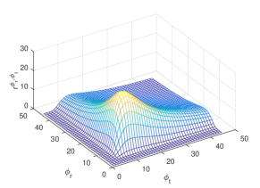
Figure 4: Link capacity for varying $\phi_{t}$, and $\phi_{r}$, $\theta_{m}=10\degree$.

IV Calculating Average Link Capacity

Generally in most of the scenarios AP/BS are fixed and mainly users’ devices are more likely to experience alignment errors. Therefore, for analytical tractability we assume that only user devices are affected by alignment errors. Hence, $\theta_{r}=\theta$ and $\theta_{t}=0$. By substituting the expressions for antenna gain in (3),

$$r^{\phi_{t},\phi_{r}}(\theta)=\eta_{\phi_{t},\phi_{r}}\log_{2}\left(1+c_{1}\exp{\left(-\left(\frac{\theta}{\phi_{r}}\right)^{2}\right)}\right).$$ (16)

For brevity, we denote $\eta_{\phi_{t},\phi_{r}}$ and $r^{\phi_{t},\phi_{r}}(\theta)$ by $\eta$ and $r$, respectively.

Since $\theta$ is assumed to be a uniformly distributed random variable interval $-\theta_{m}$ to $\theta_{m}$. Hence $r$, a function of $\theta$ ($r=g(\theta)$), also become a random variable. We represent the resulting random variable by $R$. Applying the rule of transformation of random variables [30], the pdf of $R$ represented as $f_{R}(r)$, , can be written as,

$$f_{R}(r)=(-1)^{i}f(g^{-1}(r))\frac{\partial}{\partial r}g^{-1}(r).$$ (17)

Where, $i=0$ if $g(\theta)$ is a monotonically increasing function of $\theta$, and $i=1$ if it is a monotonically decreasing function of $\theta$. It is evident from (16) that $r=g(\theta)$ is a monotonically decreasing function of $\theta$, which maximizes at $\theta=0$, and minimizes at $|\theta|=\theta_{m}$. Consequently, $i=1$ and $r$ is bounded between $g(\theta_{m})$ and $g(0)$. Using (16),

$$g^{-1}(r)={\phi_{r}}\left(\ln{\frac{2^{\frac{r}{\eta}}-1}{c_{1}}}\right)^{-\frac{1}{2}}.$$ (18)

From (6), it can be inferred that $f(g^{-1}(r))=\frac{1}{2\theta_{m}}$. Hence, the pdf of $R$ turns out as $f_{R}(r)=-\frac{\partial}{\partial r}g^{-1}(r)$. Finally, the expression for average link capacity can be written as,

$$\mathbb{E}[R]=\int_{g(\theta_{m})}^{g(0)}rf_{R}(r)dr.$$ (19)

Since $f_{R}(r)=-\frac{\partial}{\partial r}g^{-1}(r)$, (19) can be simplified as follows,

$$\mathbb{E}[R]=-\frac{1}{2\theta_{m}}\left(rg^{-1}(r)-\int{g^{-1}(r)}dr\right)\Bigg{|}_{g(\theta_{m})}^{g(0)}.$$ (20)

Since we are interested in examining the impact of alignment error on the main lobe gain, we assume that antenna pointing directions are within the -20 dBm gain directions. Therefore, we can safely assume that ${2^{\frac{r}{\eta}}>>1}$. Hence, the resulting approximate expression for $g^{-1}(r)$ from (18) is,

$$\widetilde{g}^{-1}(r)={\phi_{r}}\left(\ln{\frac{2^{\frac{r}{\eta}}}{c_{1}}}\right)^{-\frac{1}{2}}.$$ (21)

The above approximation is required to find an integrable expression for $g^{-1}(r)$ as the exact expression in (18) is not integrable. Using (21), (20) can be simplified as,

$$\mathbb{E}[R]=\frac{1}{2\theta_{m}}\left(\frac{2\phi_{r}\eta}{\ln{2}}\left(\ln{\frac{2^{\frac{r}{\eta}}}{c_{1}}}\right)^{\frac{1}{2}}-r\phi_{r}\left(\ln{\frac{2^{\frac{r}{\eta}}-1}{c_{1}}}\right)^{-\frac{1}{2}}\right)\Bigg{|}_{g(\theta_{m})}^{g(0)}.$$ (22)

Depending on the magnitude of maximum alignment error $|\theta_{m}|$ with respect to the main lobe beamwidth of user device, two scenarios are possible. We represent these scenarios using the following two propositions:

Proposition 1.

If $|\theta_{m}|\leq\frac{\phi_{ML}}{2}$, the expected link capacity is same as given by (22).

Proof.

If the maximum alignment error $|\theta_{m}|$, is less than half of main lobe beamwidth $2.6\phi$, Rx is bound to stay within its main lobe beamwidths, despite of the alignment error. Therefore, the average capacity obtained using (20) is same as represented in (22).

Proposition 2.

If $|\theta_{m}|>\frac{\phi_{ML}}{2}$, the expected link capacity is,

$$\mathbb{E}[R]= \frac{p_{\mbox{m,m}}}{2\theta_{m}}\left(\frac{2\phi_{r}\eta}{\ln{2}}\left(\ln{\frac{2^{\frac{r}{\eta}}}{c_{1}}}\right)^{\frac{1}{2}}-r\phi_{r}\left(\ln{\frac{2^{\frac{r}{\eta}}-1}{c_{1}}}\right)^{-\frac{1}{2}}\right)\Bigg{|}_{g(\theta_{m})}^{g(0)}$$

$$+p_{m,s}\eta\log_{2}\left(1+\frac{G^{\phi_{t}}_{m}G^{\phi_{r}}_{s}G_{0}(\lambda,d)P_{t}}{N_{0}W}\right),$$ (23)

here $p_{m,m}$ is the probability of both Tx and Rx staying within their main lobes and $p_{m,s}$ represents Tx staying within its mainlobe while Rx staying outside its main lobe.

Proof.

If the maximum misalignment $|\theta_{m}|>1.3\phi$, we have two cases: (i) when $|\theta|<1.3\phi$, with a probability $p_{m,m}=\left(\frac{1.3\phi_{t}}{\theta_{m}}\right)$, both Tx and Rx beams are pointing within the main lobe beamwidth. We represent the link capacity in this case by $\mathbb{E}[R||\theta|<1.3\phi]$ and as given by (22). (ii) if $|\theta_{m}|\geq|\theta|>1.3\phi$, then with probability $p_{m,s}=\left(1-\frac{1.3\phi_{t}}{\theta_{m}}\right)$, Rx antenna points in the direction of side lobe. Since, we have assumed a constant side lob gain (recall (1)), the capacity in this case, represented as $\mathbb{E}[R\mid|\theta|\geq 1.3\phi]$, can be evaluated using (3) by substituting the gain of Rx antenna by $G_{s}^{\phi_{r}}$. The link capacity can be written as $\mathbb{E}[R||\theta|\geq 1.3\phi]=\eta\log_{2}\left(1+\frac{G^{\phi_{t}}_{m}(0)G^{\phi_{r}}_{s}G_{0}(\lambda,d)P_{t}}{N_{0}W}\right)$.
Considering the above two situations, the expression for average link capacity is, $\mathbb{E}[R]=p_{m,m}\mathbb{E}[R||\theta|<1.3\phi]+p_{m,s}\mathbb{E}[R||\theta|\geq 1.3\phi]$. By replacing the corresponding capacity values ($r_{m,m}^{\phi_{t},\phi_{r}}$ and $r_{m,s}^{\phi_{t},\phi_{r}}$), (23) can be calculated.

V Numerical Results and Discussions

We use MATLAB to examine the effect of misalignment and searching overheads on mmWave link performance. We assume transmit power $P_{t}$ = 10 mW, distance between Tx and Rx $d$ = 5 m, carrier bandwidth $W$ = 2.16 GHz and the equal coarse sector beamwidth for both the Tx and Rx $\Omega$ = 90°. Using the IEEE 802.11ad specification the transmission time ${T_{p}}$ of beam-training packet is assume to be 15.6$\mu$s. The allocated slot-time duration $T_{S}$ takes two values of 10 ms and 1 s.

\psfrag{x}[cc][cc][0.80]{{Transmit and receive beamwidths (\textdegree)}}\psfrag{y}[cc][cc][0.80]{{Capacity (bits/slot/Hz)}}\includegraphics[width=95.39693pt]{Txpencilbeam_RxOmni_10ms_error_new}

(a) $T_{S}$=10 ms.

\psfrag{x}[cc][cc][0.80]{{Transmit and receive beamwidths (\textdegree)}}\psfrag{y}[cc][cc][0.80]{{Capacity (bits/slot/Hz)}}\includegraphics[width=95.39693pt]{Txpencilbeam_RxOmni_1sec_error_new}

(b) $T_{S}$e=1 s.

Figure 5: Link capacity for pencil beam reception and coarse-sector transmission.

For evaluation purpose, we consider two configurations as follows: (i)  Rx uses narrow pencil beams and Tx only employ the coarse-sector beamwidth; and (ii)  Tx and Rx both are capable of forming narrow beams with equal beamwidth $\phi$.

Fig. 5 shows the link capacity while using pencil beam reception and the coarse-sector transmission. As it can be observed from Fig. 5(a), the optimum Rx beamwidth are 3°, 7°, 10°  and 15°  for the corresponding maximum alignment errors $\theta_{m}$ of 0°, 3°, 6°  and 9°, respectively. For $\theta_{m}$ = 9°, using 15°  Rx beamwidth outperforms the 5°  beamwidth by 60%. We can also observe that as Rx beamwidth decreases, variations in link capacity are more pronounced.

Comparing Fig. 5(a) and Fig. 5(b), for the perfect alignment ($\bar{{\theta}}$ = 0°), we can see that $T_{S}$ = 1 s outperforms $T_{S}$ = 10 ms. Since the Tx employ coarse-sector beamwidth, the beam searching overhead is less impact-full when $T_{S}$=1 s and $\theta_{m}$ = 0°. Therefore, if alignment error does not exist, then using very narrow Rx beamwidth would provide the best link capacity given that sufficiently large slot is allocated for high speed data transmission and the coarse sector Tx beamwidth is used.

Fig. 6 presents the link capacity when both the Tx and Rx use narrow beamwidths. Here the misalignment sensitivity of the mmWave links is considerably higher. We can see that irrespective of the slot duration $T_{S}$, increasing the maximum alignment error $\theta_{m}$ always impacts the link capacity which is clearly seen by the large gaps in the maximum and minimum link capacity for smaller beamwidths. This proves the dominance of alignment errors over the high gain achieved by employing narrow beamwidths.

\psfrag{x}[cc][cc][0.80]{{Transmit and receive beamwidths (\textdegree)}}\psfrag{y}[cc][cc][0.80]{{Capacity (bits/slot/Hz)}}\includegraphics[width=95.39693pt]{Txpencilbeam_Rxpencil_Equal_10ms_error_new}

(a) $T_{S}$=10 ms.

\psfrag{x}[cc][cc][0.80]{{Transmit and receive beamwidths (\textdegree)}}\psfrag{y}[cc][cc][0.80]{{Capacity (bits/slot/Hz)}}\includegraphics[width=95.39693pt]{Txpencilbeam_Rxpencil_Equal_1sec_error_new}

(b) $T_{S}$=1 s.

Figure 6: Link capacity for pencil beam transmission and reception.

VI Misalignment-aware Beamwidth Adaptation Mechanism

Mechanisms that can adapt link beamwidths according to the anticipated alignment dynamics are highly desired for mmWave communications for sustained link performance. We propose a simple adaptation mechanism (see Algorithm 1) based on the observed received signal strength (RSSI) where Tx and Rx beamwidths are chosen in such a way that the link can adapt to alignment errors and a sustained link performance can be achieved. The algorithm is explained as follows.
1) The initial Tx and Rx beamwidths $\phi_{t}$ and $\phi_{r}$ are determined by Eq. (16) considering perfect alignment. In practical situations, $\phi_{t}and\phi_{r}$ would be the putcome of $2^{nd}$ stage of beam-training.
2) We define a threshold RSSI ($\mbox{RSSI}_{\mbox{th}}$). If the average RSSI ($\overline{\mbox{RSSI}}$) during a time slot falls below the threshold $\mbox{RSSI}_{\mbox{th}}$, we adapt the link beamwidth by increasing it in small-steps of $\Delta\phi$. $\mbox{RSSI}_{\mbox{th}}$ is calculated using the averaging the RSSI considering antennas pointing randomly within the entire main lobe beamwidth, i.e., $\theta\in[-1.3\phi,1.3\phi$].

$$\mbox{RSSI}_{\mbox{th}}=\frac{1}{(\frac{2.6\phi}{\Delta{\theta}}+1)}\sum_{\theta=-1.3\phi}^{1.3\phi}G_{mt}^{\phi_{t}}(\theta)G_{mr}^{\phi_{r}}(\theta)G_{0}(\lambda,d)P_{t}.$$

Here ${\Delta{\theta}}$ is the sampling interval and $\frac{1}{(\frac{2.6\phi}{\Delta{\theta}}+1)}$ is the number of steps. In our evaluations, we considered ${\Delta{\theta}}=$ 2°.
3) The beamwidth adaptation is repeated until $\overline{\mbox{RSSI}}$ reaches $\mbox{RSSI}_{\mbox{th}}$.

Algorithm 1 Beamwidth adaptation algorithm

1:  Begin with the Tx/Rx beamwidths determined by (16) without considering alignment error for the given slot duration $T_{S}$;

2:  Monitor the average signal strength $\overline{\mbox{RSSI}}$ during transmission;

3:  if $\overline{\mbox{RSSI}}<{\mbox{RSSI}}_{\mbox{th}}$ then

4:     $\phi_{t}=\phi_{t}+\Delta\phi$ and $\phi_{r}=\phi_{r}+\Delta\phi$;

5:     Go to Step 2;

6:  else

7:     Stop the beam adaptation mechanism;

8:     return  $\phi_{t},\phi_{r}$;

9:  end if

To evaluate the proposed scheme we consider two Tx/Rx beamwidth configurations. The $1^{st}$ configuration uses $\phi$=2°  and the $2nd$ uses $\phi$=7°. The initial Tx/Rx beamwidths are deduced from (16) considering $\theta=0$, slot length $T_{S}$=1 s and $T_{S}$=10 ms. All the other simulation parameters are as used in the previous section.

For beamwidth $\phi$=2° , we consider maximum alignment errors $\theta_{m}$=2°  and $\theta_{m}$=10°. For beamwidth $\phi$=7°, maximum alignment errors $\theta_{m}$=7°  and $\theta_{m}$=15°  are assumed. We run the adaptation mechanism for 10 consecutive slots. It can be inferred from Fig. 7 that the adaptation mechanism gradually attains the highest achievable capacity. In addition, the beamwidth adaptation mechanism is less likely to let the re-beamforming be invoked.

We can see that for 7°  beamwidth, the proposed mechanism considerably improves the link capacity by 20% - 100% (see Fig. 7(a) and Fig. 7(b)). For the 2°  beamwidth, similar improvements in link capacity are registered (see Fig. 7(d) and Fig. 7(d)). By comparing Fig. 7(c) and Fig. 7(d), we see that in Fig. 7(c) it takes two slots to attain the peak link capacity while in Fig. 7(d) requires five slots to attain the peak link capacity. This is the consequence of higher alignment errors in the latter case where beamwidth adaptation requires more slots to adjust the beamwidths according to the maximum alignment error. It is important to note that we have always assumed that the link deterioration is always caused by alignment errors. On the other hand, mmWave links are highly susceptible to blockage. In that case, appropriate mechanisms are required to identify if link is disrupted due to blockage or misalignment.

\psfrag{x}[cc][cc][0.80]{{Slot number}}\psfrag{y}[cc][cc][0.80]{{Capacity}}\includegraphics[width=95.39693pt]{mialignmentAlgo_BW15_mis30_infocom_lastday}

(a) ${\phi}$=7°, $\theta_{m}$=7°.

\psfrag{x}[cc][cc][0.80]{{Slot number}}\psfrag{y}[cc][cc][0.80]{{Capacity}}\includegraphics[width=95.39693pt]{mialignmentAlgo_BW15_mis45_infocom17_lastday}

(b) ${\phi}$=7°, $\theta_{m}$=15°.

\psfrag{x}[cc][cc][0.80]{{Slot number}}\psfrag{y}[cc][cc][0.80]{{Capacity}}\includegraphics[width=95.39693pt]{mialignmentAlgo_BW5_mis10_infocom17}

(c) ${\phi}$=2°, $\theta_{m}$=2°.

\psfrag{x}[cc][cc][0.80]{{Slot number}}\psfrag{y}[cc][cc][0.80]{Capacity}\includegraphics[width=95.39693pt]{mialignmentAlgo_BW5_mis20_infocom17}

(d) ${\phi}$=2°, $\theta_{m}$=10°.

Figure 7: Performance of misalignment-aware beamwidth adaptation mechanism. Here capacity is in (bits/slot/Hz).

VII Conclusion

Ultra-low latency and extreme-high reliability are two defining characteristics of Tactile Internet (TI). Since radio interface-diversity is highly desired for attaining the carrier-grade reliability in TI, Millimeter Wave (mmWave) communication is an appropriate candidates due to its unique propagation characteristics and potential for high data rate transmissions. However, using directional antennas makes mmWave susceptible to link instability and high latency. In this paper, we proposed a capacity modeling framework for the mmWave links which provided detailed insights in to the impact of using narrow beamwidth links. Our evaluations suggest that to exploit the multi-Gbps mmWave wireless links for reliable high data rate TI applications, beamwidth of directional antennas must be carefully decided. When alignment errors are likely to happen, using moderately narrow beams instead of very narrow beams is beneficial. We have also proposed a beamwidth-adaptation mechanism that is able to significantly stabilize the performance of mmWave link which is quintessential for TI applications.

In order to prove the quasi-concavity of function ${1-(\frac{{2\pi}}{{{\Omega_{t}}}}+\frac{{2\pi}}{{{\Omega_{r}}}})\frac{{{T_{p}}}}{{{T_{s}}}}-(\frac{{{\Omega_{t}}}}{{{x}}})\frac{{{T_{p}}}}{{{T_{s}}}}}$, given the theorem in (9), we consider

$$1-(\frac{{2\pi}}{{{\Omega_{t}}}}+\frac{{2\pi}}{{{\Omega_{r}}}})\frac{{{T_{p}}}}{{{T_{s}}}}-(\frac{{{\Omega_{t}}}}{x})\frac{{{T_{p}}}}{{{T_{s}}}}>a\Rightarrow x>\frac{{{\Omega_{t}}\frac{{{T_{p}}}}{{{T_{s}}}}}}{{1-(\frac{{2\pi}}{{{\Omega_{t}}}}+\frac{{2\pi}}{{{\Omega_{r}}}})\frac{{{T_{p}}}}{{{T_{s}}}}-a}}$$

$$1-(\frac{{2\pi}}{{{\Omega_{t}}}}+\frac{{2\pi}}{{{\Omega_{r}}}})\frac{{{T_{p}}}}{{{T_{s}}}}-(\frac{{{\Omega_{t}}}}{y})\frac{{{T_{p}}}}{{{T_{s}}}}>a\Rightarrow y>\frac{{{\Omega_{t}}\frac{{{T_{p}}}}{{{T_{s}}}}}}{{1-(\frac{{2\pi}}{{{\Omega_{t}}}}+\frac{{2\pi}}{{{\Omega_{r}}}})\frac{{{T_{p}}}}{{{T_{s}}}}-a}}$$ (24)

Therefore,

$$\lambda x+(1-\lambda)y>\frac{{{\Omega_{t}}\frac{{{T_{p}}}}{{{T_{s}}}}}}{{1-(\frac{{2\pi}}{{{\Omega_{t}}}}+\frac{{2\pi}}{{{\Omega_{r}}}})\frac{{{T_{p}}}}{{{T_{s}}}}-a}}$$

$$\Rightarrow 1-(\frac{{2\pi}}{{{\Omega_{t}}}}+\frac{{2\pi}}{{{\Omega_{r}}}})\frac{{{T_{p}}}}{{{T_{s}}}}-(\frac{{{\Omega_{t}}}}{{\lambda x+(1-\lambda)y}})\frac{{{T_{p}}}}{{{T_{s}}}}>a.$$

In addition, we need to prove that ${1-(\frac{{2\pi}}{{{\Omega_{t}}}}+\frac{{2\pi}}{{{\Omega_{r}}}})\frac{{{T_{p}}}}{{{T_{s}}}}-(\frac{{{\Omega_{t}}}}{{{x}}})\frac{{{T_{p}}}}{{{T_{s}}}}}$ is also nonnegative. In order to have that,

$$x\geq\frac{{{\Omega_{t}}}}{{\frac{{{T_{p}}}}{{{T_{s}}}}-(\frac{{2\pi}}{{{\Omega_{t}}}}+\frac{{2\pi}}{{{\Omega_{r}}}})}}$$ (25)

should hold. Given the value of the parameters $T_{p}$, $T_{s}$, $\Omega_{t}$ and $\Omega_{r}$, the right hand side of the inequality is always negative. Therefore, (25) holds.

References

- [1] G. P. Fettweis, “The Tactile Internet: Applications and challenges,” IEEE Vehicular Technology Magazine, vol. 9, no. 1, pp. 64–70, 2014.
- [2] O. Holland, E. Steinbach, R. V. Prasad, Q. Liu, Z. Dawy, A. Aijaz, N. Pappas, K. Chandra, V. S. Rao, S. Oteafy, M. Eid, M. Luden, A. Bhardwaj, X. Liu, J. Sachs, and J. Araújo, “The ieee 1918.1 “tactile internet” standards working group and its standards,” Proceedings of the IEEE, vol. 107, no. 2, pp. 256–279, Feb 2019.
- [3] A. Aijaz, M. Dohler, A. H. Aghvami, V. Friderikos, and M. Frodigh, “Realizing the tactile Internet: Haptic communications over next generation 5G cellular networks,” IEEE Wireless Communications, vol. 24, no. 2, pp. 82–89, 2017.
- [4] P. Popovski, J. J. Nielsen, C. Stefanovic, E. d. Carvalho, E. Strom, K. F. Trillingsgaard, A. Bana, D. M. Kim, R. Kotaba, J. Park, and R. B. Sorensen, “Wireless Access for Ultra-Reliable Low-Latency Communication: Principles and Building Blocks,” IEEE Network, vol. 32, no. 2, pp. 16–23, March 2018.
- [5] G. Durisi, T. Koch, and P. Popovski, “Toward Massive, Ultrareliable, and Low-Latency Wireless Communication With Short Packets,” Proceedings of the IEEE, vol. 104, no. 9, pp. 1711–1726, Sep. 2016.
- [6] G. Pocovi, B. Soret, K. I. Pedersen, and P. Mogensen, “MAC layer enhancements for ultra-reliable low-latency communications in cellular networks,” in 2017 IEEE International Conference on Communications Workshops (ICC Workshops), May 2017, pp. 1005–1010.
- [7] F. Boccardi, R. Heath, A. Lozano, T. Marzetta, and P. Popovski, “Five disruptive technology directions for 5G,” Communications Magazine, IEEE, vol. 52, no. 2, pp. 74–80, February 2014.
- [8] K. Chandra, R. V. Prasad, B. Quang, and I. G. M. M. Niemegeers, “Cogcell: cognitive interplay between 60 ghz picocells and 2.4/5 ghz hotspots in the 5g era,” IEEE Communications Magazine, vol. 53, no. 7, pp. 118–125, July 2015.
- [9] W. Roh, J.-Y. Seol, J. Park, B. Lee, J. Lee, Y. Kim, J. Cho, K. Cheun, and F. Aryanfar, “Millimeter-wave beamforming as an enabling technology for 5G cellular communications: theoretical feasibility and prototype results,” Communications Magazine, IEEE, vol. 52, no. 2, pp. 106–113, February 2014.
- [10] A. W. Doff, K. Chandra, and R. V. Prasad, “Sensor assisted movement identification and prediction for beamformed 60 ghz links,” in 2015 12th Annual IEEE Consumer Communications and Networking Conference (CCNC), Jan 2015, pp. 648–653.
- [11] H. D. Schotten, R. Sattiraju, D. G. Serrano, Z. Ren, and P. Fertl, “Availability indication as key enabler for ultra-reliable communication in 5G,” in 2014 European Conference on Networks and Communications (EuCNC), June 2014, pp. 1–5.
- [12] “IEEE working group, tgc3,,” Report.
- [13] “Draft standard- part 11: Wireless lan medium access control (mac) and physical layer (phy) specifications - amendment 4: Enhancements for very high throughput in the 60ghz band,” IEEE P802.11adTM/D9.0, July 2012.
- [14] R. Ford, M. Zhang, M. Mezzavilla, S. Dutta, S. Rangan, and M. Zorzi, “Achieving Ultra-Low Latency in 5G Millimeter Wave Cellular Networks,” IEEE Communications Magazine, vol. 55, no. 3, pp. 196–203, March 2017.
- [15] G. Yang and M. Xiao and M. Alam and Y. Huang, “Low-Latency Heterogeneous Networks with Millimeter-Wave Communications,” IEEE Communications Magazine, vol. 56, no. 6, pp. 124–129, June 2018.
- [16] G. Yang, M. Xiao, and H. V. Poor, “Low-Latency Millimeter-Wave Communications: Traffic Dispersion or Network Densification?” IEEE Transactions on Communications, vol. 66, no. 8, pp. 3526–3539, Aug 2018.
- [17] T. K. Vu, C. Liu, M. Bennis, M. Debbah, M. Latva-aho, and C. S. Hong, “Ultra-Reliable and Low Latency Communication in mmWave-Enabled Massive MIMO Networks,” IEEE Communications Letters, vol. 21, no. 9, pp. 2041–2044, Sep. 2017.
- [18] Jain, Ish Kumar and Kumar, Rajeev and Panwar, Shivendra, “Can Millimeter Wave Cellular Systems provide High Reliability and Low Latency? An analysis of the impact of Mobile Blockers,” arXiv preprint arXiv:1807.04388, 2018.
- [19] K. Chandra, R. V. Prasad, I. G. M. M. Niemegeers, and A. R. Biswas, “Adaptive beamwidth selection for contention based access periods in millimeter wave wlans,” in 2014 IEEE 11th Consumer Communications and Networking Conference (CCNC), Jan 2014, pp. 458–464.
- [20] K. Chandra, R. V. Prasad, and I. Niemegeers, “Performance analysis of ieee 802.11ad mac protocol,” IEEE Communications Letters, vol. 21, no. 7, pp. 1513–1516, July 2017.
- [21] B. Li, Z. Zhou, W. Zou, X. Sun, and G. Du, “On the Efficient Beam-Forming Training for 60GHz Wireless Personal Area Networks,” Wireless Communications, IEEE Transactions on, vol. 12, no. 2, pp. 504–515, February 2013.
- [22] T. Nitsche, A. Flores, E. Knightly, and J. Widmer, “Steering with Eyes Closed: mm-Wave Beam Steering without In-Band Measurement,” in Proceedings of IEEE INFOCOM, April 2015.
- [23] H. S. Ghadikolaei, L. Gkatzikis, and C. Fischione, “Beam-searching and transmission scheduling in millimeter wave communications,” IEEE ICC, 2015. [Online]. Available: http://arxiv.org/abs/1501.02516
- [24] J. Wildman, P. Nardelli, M. Latva-Aho, and S. Weber, “On the Joint Impact of Beamwidth and Orientation Error on Throughput in Directional Wireless Poisson Networks,” Wireless Communications, IEEE Transactions on, vol. 13, no. 12, pp. 7072–7085, Dec 2014.
- [25] A. Thornburg and R. W. Heath, “Ergodic capacity in mmWave ad hoc network with imperfect beam alignment,” in Military Communications Conference, MILCOM 2015 - 2015 IEEE, Oct 2015, pp. 1479–1484.
- [26] X. Yu, J. Zhang, M. Haenggi, and K. B. Letaief, “Coverage analysis for millimeter wave networks: The impact of directional antenna arrays,” IEEE journal on selected areas in communications, vol. 35, no. 7, pp. 1498–1512, 2017.
- [27] C. Liu, M. Li, S. V. Hanly, I. B. Collings, and P. Whiting, “Millimeter wave beam alignment: Large deviations analysis and design insights,” IEEE journal on selected areas in communications, vol. 35, no. 7, pp. 1619–1631, 2017.
- [28] S. Boyd and L. Vandenberghe, Convex optimization. Cambridge university press, 2009.
- [29] M. Kopa and P. Lachout, “Characterization of uniformly quasi-concave functions,” in Proceedings of the 30th International Conference on Mathematical Methods in Economics, Karviná, Silesian University in Opava, 2012, pp. 449–454.
- [30] G. Grimmett and D. Stirzaker, Probability and random processes. Oxford university press, 2001.