Real Time Trajectory Prediction Using Deep Conditional Generative Models

Abstract

Data driven methods for time series forecasting that quantify uncertainty open new important possibilities for robot tasks with hard real time constraints, allowing the robot system to make decisions that trade off between reaction time and accuracy in the predictions. Despite the recent advances in deep learning, it is still challenging to make long term accurate predictions with the low latency required by real time robotic systems. In this paper, we propose a deep conditional generative model for trajectory prediction that is learned from a data set of collected trajectories. Our method uses encoder and decoder deep networks that map complete or partial trajectories to a Gaussian distributed latent space and back, allowing for fast inference of the future values of a trajectory given previous observations. The encoder and decoder networks are trained using stochastic gradient variational Bayes. In the experiments, we show that our model provides more accurate long term predictions with a lower latency than popular models for trajectory forecasting like recurrent neural networks or physical models based on differential equations. Finally, we test our proposed approach in a robot table tennis scenario to evaluate the performance of the proposed method in a robotic task with hard real time constraints.

I INTRODUCTION

Dynamic high speed robotics tasks often require accurate methods to forecast the future value of a physical quantity based on previous measurements while respecting the real time constraints of the particular application. For example, to hit or catch a flying ball with a robotic system we need to predict accurately and fast the trajectory of the ball based on previous observations that are often noisy and might include outliers or missing observations. Note that the time it takes to compute the predictions, called latency, is as important for the application as the accuracy in the prediction. In our previous example, the prediction of the future ball positions are only useful if the computation time is significantly faster than the ball itself.

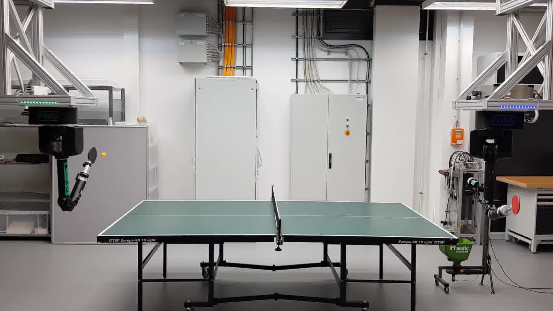
Figure 1: Robot table tennis setup used to evaluate the trajectory forecasting methods. The ball is tracked using four VGA resolution cameras attached to the ceiling with a sampling frequency of 180 frames per second. The robot arms are Barrett WAM capable of high speed motion with seven degrees of freedom.

Both physics-based [19] and data-driven [2] models are used for trajectory forecasting. Physical models based on differential equations have been typically preferred to model and predict trajectories in high speed robotic systems [12], because they are relatively fast for predictions and are well studied models known to provide reasonably good predictions for many problems. However, in some applications like pneumatic muscle robots [3], the best known physic-based models are not accurate enough to be useful for control. Even in cases where the physics are relatively well known, estimating all the relevant variables to model the system can be difficult. In table tennis, for example, estimating the spin of the ball in real time from images is hard. In addition, small lens distortion on the vision system makes the position estimates not equally accurate in all the robot work space, rendering the estimation of the initial position and velocity less accurate. A data-driven approach, on the other hand, may have the potential to estimate the spin from its effect on the trajectory and ignore the lens distortion as long as it is present both at training and test time. However, popular data-driven methods for time series modeling like recurrent neural networks [14] and auto-regressive models [2] suffer from cumulative errors that render trajectory forecasting inaccurate as we predict farther into the future.

Figure 2: Example of a ball trajectory in X, Y and Z (in meters) with respect to time (in seconds) and the respective prediction using LSTMs and the proposed method (TVAE). The observed ball trajectory is depicted in red, the prediction using a LSTM is depicted in green, and the prediction using the proposed model is depicted in blue. The shaded area corresponds to one standard deviation. Note the cumulative error effect. The error grows very large for LSTMs as we predict farther into the future. The proposed method is more accurate for long term predictions.

In this paper, we propose a novel method for trajectory prediction that mixes the power of deep learning and conditional generative models to provide a data-driven approach for accurate trajectory forecasting with the low latency required by real time applications. We follow a similar approach to conditional variational auto-encoders [16], using a latent variable $\boldsymbol{z}$ to represent an entire trajectory, as well as an encoder and decoder network to map trajectories to and from the latent representation $\boldsymbol{z}$. Our model is trained to maximize the conditional log-likelihood of the future observations given the past observations, using stochastic gradient descent and reparametrization for the optimization [11] of the variational objective. In addition, we introduce strategies to make the model robust to missing observations and outliers. We evaluate the proposed approach on a robot table tennis setup in simulation and in the real system, showing a higher prediction accuracy than a LSTM recurrent neural network [10] and a physics-based model [4], while achieving real time execution performance. An open-source implementation of the method presented in this paper is provided [15]. Figure 1, shows an image of the robot system used in the experiments, consisting of two Barrett WAM robot arms capable of high speed movement, and a vision system [8] using four cameras with a frequency of 180 frames per second.

II TRAJECTORY PREDICTION

The term trajectory is commonly used in the robotics community to refer to a realization of a time series or Markov decision process. Formally, we define a trajectory $\tau_{n}=\{\boldsymbol{y}_{t}^{n}\}_{t=1}^{T_{n}}$ of total length $T_{n}$ as a sequence of multiple observations $\boldsymbol{y}_{t}^{n}$, where the index $t$ represents time and $n$ indexes the different trajectories in the data set. For example, for the table tennis ball prediction problem, the observation $\boldsymbol{y}_{t}^{n}$ is a 3 dimensional vector representing the ball position at time index $t$ of the ball trajectory $n$.

Each trajectory $\tau_{n}\sim P(\tau)$ is assumed to be independently sampled from the trajectory distribution $P(\tau)$. For trajectory prediction, we need to be able to predict the future trajectory based on previous observations. Let us use $\boldsymbol{y}_{t}$ to denote the random variable representing the observation indexed by time $t$ in any trajectory. Formally, the goal of trajectory forecasting is to compute the conditional distribution $p(\boldsymbol{y}_{t},\dots,\boldsymbol{y}_{T}\,|\,\boldsymbol{y}_{1},\dots,\boldsymbol{y}_{t-1})$, representing the distribution of the future values of a trajectory $\{\boldsymbol{y}_{t},\dots,\boldsymbol{y}_{T}\}$ given the previous observations $\{\boldsymbol{y}_{1},\dots,\boldsymbol{y}_{t-1}\}$. From this point on, we will use $\boldsymbol{y}_{1:t}$ to denote the set of variables $\{\boldsymbol{y}_{1},\dots,\boldsymbol{y}_{t}\}$ compactly.

Trajectory or time series forecasting methods is an active research area of machine learning. Examples of popular approaches for time series forecasting include recurrent neural networks [14], auto-regressive models [2, 17] and state space models [5]. Some of which include real time performance considerations [13]. All these approaches share in common that they model $p(\boldsymbol{y}_{t}\,|\,\boldsymbol{y}_{1:t-1})$, and use the factorization property of probability theory

$$p(\boldsymbol{y}_{t:T}\,|\,\boldsymbol{y}_{1:t-1})=\prod_{i=t}^{T}{p(\boldsymbol{y}_{i}\,|\,\boldsymbol{y}_{1:i-1})},$$

to model and predict the entire future trajectory from past observations. Note that these models predict directly only one observation into the future $\boldsymbol{y}_{i}$ given the past $\boldsymbol{y}_{1:i-1}$. To make predictions farther into the future, the predictions of the model are fed back into the model as additional input observations. We will call an approach for trajectory forecasting “recursive” if it uses its own predictions as input to predict farther into the future.

An advantage of the recursive approaches is that they can model sequences of arbitrary length by design. It is always possible to make predictions with any given number of observations for any arbitrary number of time steps into the future. On the other hand, the recursive approaches have the disadvantage that errors are cumulative. Note that the predictions of the recursive approaches are fed back into the model. As a result, early small prediction errors can cause big forecasting errors as we try to predict farther into the future. For problems with high stochasticity like traffic [18], weather or stock market price prediction [2], where some of these models are commonly applied, it is reasonable to assume that no method will ever make almost exact long term predictions based only in previous observations.

However, for trajectory prediction in physical systems, where we are measuring all the relevant variables, we would expect long term prediction to be more accurate. For example, we know that the model used to generate the table tennis ball trajectories in simulation is deterministic once the initial state is set. However, the long term prediction error using an LSTM [10] recurrent neural network is about twice as large as using the physics-based model. Figure 2 shows an example ball trajectory and the model predictions using an LSTM, depicted in green. The cumulative error effect for the LSTM model is easy to notice, specially in the Y coordinate, where the predictions deviate early from the ground truth ball trajectory depicted in red.

III DEEP CONDITIONAL GENERATIVE MODELS FOR TRAJECTORY FORECASTING

We have discussed how recursive methods like recurrent neural networks suffer from cumulative errors that render long term predictions less accurate. Therefore, our goal is to find a way to represent the conditional distribution $p(\boldsymbol{y}_{t:T}\,|\,\boldsymbol{y}_{1:t-1})$ directly, in a way where the model predictions are not fed back into the model. In addition, we want to use a powerful model that can capture non linear relationships between the future and the past observations.

III-A Deterministic Regression Using Input Masks

Note that for a fixed value $t$, we could model $p(\boldsymbol{y}_{t:T}\,|\,\boldsymbol{y}_{1:t-1})$ directly as a regression problem. If we use a complex non-linear regression model such as a neural network, we can capture non linear relations between the past and future observations. To deal with a variable number of inputs $t$ and outputs $T-t$, we use two auxiliary input variables $\boldsymbol{x}^{t}$ and $\hat{\boldsymbol{x}}^{t}$ that represent a zero-padded input observations and an observation mask. Given a set of observations $\boldsymbol{y}_{1:t-1}$ we set $\boldsymbol{x}_{1:t-1}^{t}=\boldsymbol{y}_{1:t-1}$, $\boldsymbol{x}_{t:T}^{t}=\boldsymbol{0}$, $\hat{\boldsymbol{x}}_{1:t-1}^{t}=1$ and $\hat{\boldsymbol{x}}_{t:T}^{t}=0$. The variable $\boldsymbol{x}^{t}$, represents the observations seen so far, padding the non-observed part of the trajectory with zeros. Similarly, the variable $\hat{\boldsymbol{x}}^{t}$ represents a {0,1} mask indicating which values were observed and which values were not. Using the auxiliary variables $\boldsymbol{x}^{t}$ and $\hat{\boldsymbol{x}}^{t}$ we can make predictions with any number of input observations $t\in\{0,1,\dots,T\}$ using a single regression model even if we have missing observations.

The proposed approach assumes a fixed maximum prediction horizon $T$ for all trajectories. This is a limitation for our approach compared to all the recursive models, that can model trajectories of any duration. We trade the flexibility of being able to model trajectories of arbitrary duration for higher accuracy in the predictions and faster computation times. In Section III-F, we discuss ideas to mix the power of the proposed method with recursive approaches to be able to make predictions of any arbitrary duration.

III-B Capturing Uncertainty and Variability

(a) Encoder network

(b) Decoder network

Figure 3: Encoder and decoder networks for the proposed approach. The encoder network takes as input the past observations encoded in the variables $(\boldsymbol{x}^{t},\hat{\boldsymbol{x}}^{t})$ and produces a Gaussian distribution for the latent variable $\boldsymbol{z}$ with mean $\boldsymbol{\mu}_{z}$ and standard deviation $\boldsymbol{\sigma}_{z}$. The decoder network takes a sample $\boldsymbol{z}$ and the past observations and produces a trajectory estimate $\hat{\boldsymbol{y}}$ including both the future $\hat{\boldsymbol{y}}_{t:T}$ and the past $\hat{\boldsymbol{y}}_{1:t-1}$.

Quantifying the uncertainty of the trajectory predicted by the model is important for decision making. A self-driving car, for example, could reduce the speed if there is high uncertainty about the trajectory of a pedestrian crossing the street. For real time systems, the ability to quantify uncertainty allows the agent to make decisions that compromise between accuracy and time to react. In robot table tennis, for example, the robot could wait for more ball observations if there is high uncertainty about the ball trajectory, but waiting too long will result in failure to hit the ball.

We capture uncertainty about the predictions of a trajectory $\tau_{n}$ using a latent variable $\boldsymbol{z}^{n}$, that can be mapped to a trajectory using a complex non-linear function, similarly to other deep generative models approaches [7] like variational auto-encoders. We assume that the future observations $\boldsymbol{y}_{t:T_{n}}^{n}$ are independent given the latent variable $\boldsymbol{z}^{n}$ and the previous observation $\boldsymbol{y}_{1:t-1}^{n}$, and are distributed by

$$p(\boldsymbol{y}_{t:T}^{n}\,|\,\boldsymbol{y}_{1:t-1}^{n},\boldsymbol{z})=\prod_{i=t}^{T_{n}}\mathcal{N}\left({\boldsymbol{y}_{i}^{n}}\,\left|\,{\hat{\boldsymbol{y}}_{i}^{n}},{\boldsymbol{\Sigma}_{y}}\right.\right),$$ (1)

where $\hat{\boldsymbol{y}}^{n}$ is the estimated trajectory produced by the decoder network $\boldsymbol{f}_{\theta}$ and $\boldsymbol{\Sigma}_{y}$ represents the observation noise learned also from data.

We want to emphasize that the limitation of a fixed prediction horizon $T$ means that we do not have a principled approach to make predictions beyond $T$, but we can train our model with trajectories of any length $T_{n}$. If a trajectory $\tau_{n}$ with length $T_{n}<T$ is sampled in the training mini-batch, the model still predicts a trajectory of length $T$ but the predictions with $t>T_{n}$ are not “penalized” as can be seen in (1). Note that the likelihood is evaluated for observations until $T_{n}$. If on the other hand $T_{n}\geq T$, we cut a random time interval $[t_{a},t_{b}]$ such that $T=t_{b}-t_{a}$ for that particular mini-batch. When the same trajectory is drawn in a mini-batch later in the training process, a different random time interval $[t_{a},t_{b}]$ is used. The training procedure is explained with greater detail in Section III-D, the main message of this paragraph is that we can train our model with a data set of trajectories of any length. In Section III-F, we mention possible ideas to make predictions beyond the time horizon $T$ by mixing the advantages of recursive approaches with the method presented on this paper. We will drop the trajectory index $n$ from the notation from this point forward to avoid notational clutter.

Our approach, based on variational auto-encoders, will use an encoder and decoder network to make predictions about the future value of a trajectory. The decoder network, depicted in Figure 3(b), takes as input the previous observations $\boldsymbol{y}_{1:t-1}$ represented by $(\boldsymbol{x}^{t},\hat{\boldsymbol{x}}^{t})$ as well as the latent variable $\boldsymbol{z}$ that encodes one of the possible future trajectories. The output of the decoder network $\hat{\boldsymbol{y}}$ contains the predicted value for the future observations $\boldsymbol{y}_{t:T}$. We also use an encoder network $\boldsymbol{g}_{\phi}$ that produces the variational distribution $q_{\phi}(\boldsymbol{z}\,|\,\boldsymbol{y}_{1:t})$. The encoder network encodes a partial trajectory with observations $\boldsymbol{y}_{1:t}$ to the latent space $\boldsymbol{z}$.

III-C Inference

At prediction time, we typically want to draw several samples of the future trajectory conditioned on the previous observations $p(\boldsymbol{y}_{t:T}\,|\,\boldsymbol{y}_{1:t-1})$. To do so, we compute first the latent space distribution $p(\boldsymbol{z}\,|\,\boldsymbol{y}_{1:t-1})$ by passing the given observations through the encoder network $\boldsymbol{g}_{\phi}$. Figure 3(a) shows a diagram of the encoder network. Given the previous observations, the encoder provides us with a mean $\boldsymbol{\mu}_{z}$ and standard deviation $\boldsymbol{\sigma}_{z}$ vector for the latent variable $\boldsymbol{z}$. Subsequently, we sample several values $\boldsymbol{z}^{l}\sim\mathcal{N}\left({\boldsymbol{z}}\,\left|\,{\boldsymbol{\mu}_{z}},{\boldsymbol{\sigma}_{z}}\right.\right)$. Each sample $\boldsymbol{z}^{l}$ and the previous ball observations are passed through the decoder network to obtain a sample future trajectory.

The inference process at prediction time is therefore very efficient. It requires a single pass through the encoder and the decoding process for every sample $\boldsymbol{z}^{l}$ can be done in parallel. In contrast with recurrent neural networks, the prediction process can be easily parallelized, allowing fast execution even for relatively large deep learning models.

(a) Prediction error in simulation

(b) Prediction error in the real system

Figure 4: Distribution of the error in the test set for simulated data and real data as a function of the number of observation to predict into the future. Note that in simulated data our model performs as well as the differential equation based prediction, which was the model used in simulation and therefore is the best we can get. In real data, our model outperforms both the LSTM and differential equation models, specially as we predict farther into the future.

III-D Training Procedure

The conditional likelihood using the latent variable $\boldsymbol{z}$ is given by

$$p(\boldsymbol{y}_{t:T}\,|\,\boldsymbol{y}_{1:t-1})=\int{p(\boldsymbol{y}_{t:T}\,|\,\boldsymbol{y}_{1:t-1},\boldsymbol{z})p(\boldsymbol{z}\,|\,\boldsymbol{y}_{1:t-1})d\boldsymbol{z}},$$ (2)

with $p(\boldsymbol{y}_{t:T}\,|\,\boldsymbol{y}_{1:t-1},\boldsymbol{z})$ given by (1). We use the encoder network $\boldsymbol{g}_{\phi}$ to compute $p(\boldsymbol{z}\,|\,\boldsymbol{y}_{1:t-1})$. In many applications, it is important to make sure the latent variable encodes all the relevant information about the previous observations, in which case the decoder distribution $p(\boldsymbol{y}_{t:T}\,|\,\boldsymbol{y}_{1:t-1},\boldsymbol{z})=p(\boldsymbol{y}_{t:T}\,|\,\boldsymbol{z})$. We present the math of the model without making the previous assumption of conditional independence for generality. Incorporating the conditional independence assumption is trivial: simply ignore the input $(\boldsymbol{x}^{t},\hat{\boldsymbol{x}}^{t})$ when evaluating the decoder network $\boldsymbol{f}_{\theta}$. In the experimental section, we compare the results with and without assuming conditional independence for the table tennis ball prediction problem, showing a slight improvement in generalization performance using the conditional independence assumption.

The integral required to evaluate the conditional likelihood in (2) is intractable. We follow the approach used for Conditional Variational Auto-Encoders [16] (CVAE), optimizing instead a variational lower bound on the conditional log likelihood given by

$$\begin{split}&\log{p_{\theta}(\boldsymbol{y}_{t:T}\,|\,\boldsymbol{y}_{1:t-1})}\geq-\operatorname{KL}(q_{\phi}(\boldsymbol{z}\,|\,\boldsymbol{y}_{1:T})\|q_{\phi}(\boldsymbol{z}\,|\,\boldsymbol{y}_{1:t-1}))\\ &\quad+\operatorname{\mathbb{E}}_{q_{\phi}(\boldsymbol{z}\,|\,\boldsymbol{y}_{1:T})}[\log{p(\boldsymbol{y}_{t:T}\,|\,\boldsymbol{y}_{1:t},\boldsymbol{z})}],\end{split}$$ (3)

where $q_{\phi}(\boldsymbol{z}\,|\,\boldsymbol{y}_{1:T})$ is the variational distribution given by

$$q_{\phi}(\boldsymbol{z}\,|\,\boldsymbol{y}_{1:T})=\prod_{k=1}^{K}{\mathcal{N}\left({z_{k}}\,\left|\,{\mu_{z}^{k}},{\sigma_{z}^{k}}\right.\right)},$$

with $\boldsymbol{\mu}_{z}$ and $\boldsymbol{\sigma}_{z}$ produced by the encoder network and $K$ is the size of the latent vector $\boldsymbol{z}$. The derivation of this objective function is presented in the supplementary material. The first term of the objective keeps the distributions of $\boldsymbol{z}$ for partial trajectory and complete trajectories close. The second term forces the latent representation to be a good predictor for the future trajectory. The KL divergence term can be computed in closed form since both $q_{\phi}(\boldsymbol{z}\,|\,\boldsymbol{y}_{1:T})$ and $q(\boldsymbol{z}\,|\,\boldsymbol{y}_{1:t-1})$ are Gaussian distributions. The expectation is approximated with Montecarlo by sampling $\boldsymbol{z}$ from the variational distribution $q_{\phi}(\boldsymbol{z}\,|\,\boldsymbol{y}_{1:T})$. Note that the only difference between optimizing the second term on (3) and optimizing (2) is that the expectation is computed over a complete or a partial trajectory respectively. This difference is key to compute the expectation using Montecarlo. The distribution over $\boldsymbol{z}$ using partial trajectories is typically too broad to be efficiently and accurately approximated using Montecarlo, specially when the cut point $t$ is small.

Similarly to other deep generative models like variational auto-encoders, the lower bound on (3) can be optimized using stochastic gradient descent to find the encoder $\boldsymbol{\phi}$ and decoder $\boldsymbol{\theta}$ network parameters. The “reparametrization trick” [11] is used to compute gradients. We provide an open source implementation of the proposed method available in [15]. The training set consists of a set of trajectories $\tau_{n}$ each of a possibly different length $T_{n}$. When we sample mini-batches to train our model, we randomly select a cut point $t$ for the trajectory $\tau_{n}$ with $0<t\leq\tau_{n}$, and compute the lower bound for $p(\boldsymbol{y}_{t:T}\,|\,\boldsymbol{y}_{1:t-1})$ using the particular cut point $t$. That way, our model will learn to make predictions for any number of given observations, including an empty set of observations. Finally, to make our model more robust to missing observations or outliers, we can randomly generate missing observations and outliers for the previous observations $\boldsymbol{y}_{1:t-1}$ in each of the trajectories included in the training mini-batch. To generate outliers we simply replace an observation with a random value within the domain of the input. We provide an open source implementation of the training procedure presented in this section on [15], using Keras [6] and TensorFlow [1].

III-E Network Architecture

The approach presented on this paper can be used with any regression method for $\boldsymbol{f}_{\theta}$ and $\boldsymbol{g}_{\phi}$ as long as we can compute derivatives $\frac{d\boldsymbol{f}_{\theta}}{d\boldsymbol{\theta}}$ and $\frac{d\boldsymbol{g}_{\phi}}{d\boldsymbol{\phi}}$. We used neural networks for this purpose in our experiments. We think that convolutional network architectures have great potential for time series or trajectory forecasting applications, since observations close in time are typically more strongly correlated than observations farther apart. Note that convolutional architectures have also been quite successful on image recognition applications, where pixels spatially close are typically also more strongly correlated.

For the experiments on this paper, we only used two layer architectures with dense connections for simplicity. The number of neurons on the hidden layer and the dimensionality of the latent space $\boldsymbol{z}$ were selected by testing multiple powers of two and selecting the hyper-parameters with better performance on the validation set.

III-F Predicting Beyond the Horizon $T$

There may be many applications where making predictions arbitrarily far into the future is very important. Suppose for example that you use the presented approach to learn a forward model of a robot, and the goal is to use it to train a reinforcement learning agent in simulation. In such a case it is important to be able to make predictions much farther into the future, even at the expense of loosing accuracy.

The presented approach could be extended with ideas from recursive approaches to make predictions far into the future. The simplest recursive idea would be to use our model in an auto-regressive way, as it would require no change to the math or software implementation. In auto-regressive mode, we would simply use the predictions of our model as input observations.

A possibly better approach would be to use a state space model or recurrent neural network over the latent variable $\boldsymbol{z}$ representing block of observations. This approach would require to modify the encoder to receive the latent representation of the previous block $i-1$ of $T$ observations in addition to the observations seen so far on the current block $i$. The encoder distribution would be therefore represented as $p(\boldsymbol{z}_{i}\,|\,\boldsymbol{z}_{i-1},\boldsymbol{y}_{iT:iT+t})$. We do not explore any of these options in this paper but consider evaluating these approaches important future work.

IV EXPERIMENTS

We evaluate the proposed method to predict the trajectory of a table tennis ball in simulation and in a real robot table tennis system. Predicting accurately the trajectory of a table tennis ball is difficult mostly because the spin is not directly observed by the vision system [8], but is significant due to the low mass of the ball.

We measure the prediction error and the latency, both important factors for real time robot applications. We use “TVAE” (Trajectory Variational Auto-Encoder) to abbreviate the name of the proposed method. We compare the results with an LSTM and the physics-based differential equation prediction.

For the differential equation method, we use the ball physics proposed in [12]. This physics model considers air drag and bouncing physics but ignores spin. To estimate the initial position and velocity, we use the approach proposed in [4], that consists on fitting a polynomial to the first $n$ observations and evaluating the polynomial of degree $k$ and its derivative in $t=0$. We selected $n=30$ and $k=2$ that provided the highest predictive performance on our training data set.

To measure the prediction latency, we used a Lenovo Thinkpad X1 Carbon with an Intel 4 Core i7 6500U CPU of 2.50GHz and 8 GB of RAM memory.

IV-A Prediction Accuracy in Simulation

The simulation uses the same differential equation we used on the physics-based model. The results should be optimal for the physics-based model on simulation, where the only source of error is the initial position and velocity estimation from noisy ball observations. To simulate the average position estimation error of the vision system [8] in simulation, we added Gaussian white noise with a standard deviation of 1 cm.

We generated 2000 ball trajectories for training, and another 200 for the test set. Figure 4(a) shows the prediction error (mean and standard deviation) in simulation over the test set. Note that the error distribution of the proposed method and the physics-based model is almost identical, which is remarkable provided that the physics model used for the simulator and the differential equation predictor are the same. The results of the LSTM are slightly better than the proposed model for the first 10 observations into the future, but the error for long term prediction is about three times as large as the error for the physics or the proposed model.

Figure 5: Prediction error on the test set assuming conditional independence (TVAE CI) between the future and the past given the latent variable $\boldsymbol{z}$ and without any assumptions (TVAE Full). Using conditional independence forces the model to represent all the information about the past in the latent variable. Although both error curves are similar, assuming conditional independence $p(\boldsymbol{y}_{t:T}\,|\,\boldsymbol{z},\boldsymbol{y}_{1:t-1})=p(\boldsymbol{y}_{t:T}\,|\,\boldsymbol{z})$ presented a smaller average generalization error.

IV-B Prediction Accuracy in the Real System

The real system consists of four RGB cameras taking 180 pictures per second attached to the ceiling. The images are processed with the stereo vision system proposed in [8], obtaining estimations of the position of the ball. There are several issues that make ball prediction harder on the real system: There are missing observations, the error is not the same in all the space due to the effects of lens distortion, and the ball spin can not be observed directly. We used the vision system to collect a data set of ball trajectories including as much variability as possible, throwing balls with the hand, with a mechanical ball launcher, and hitting them with a table tennis racket. We randomly permuted the collected ball trajectory order and subsequently selected the first 614 trajectories for the training set and 35 trajectories for the test set. The training algorithm further splits the training set into a 90% for actual training and a remaining 10% for the validation set used to optimize the model hyper-parameters. For both our model and the LSTM, we used latent variable $\boldsymbol{z}$ of size 64, which was the power of two values with better validation performance. In the supplementary material and in our software repository [15], you will find the data sets collected and used for this experiments, along with a Python script to plot a small subset of trajectories. The trajectories have typically a duration between 0.8 and 1.2 seconds. We used a time horizon of $T=1.2$ seconds for our experiments.

First, let us compare the generalization error of the presented model with and without making the conditional independence assumption $p(\boldsymbol{y}_{t:T}\,|\,\boldsymbol{z},\boldsymbol{y}_{1:t-1})=p(\boldsymbol{y}_{t:T}\,|\,\boldsymbol{z})$. Figure 5 shows the prediction error on the test set collected on the real system with (TVAE CI) and without (Full TVAE) this conditional independence assumption, given the first 30 observations. Assuming $p(\boldsymbol{y}_{t:T}\,|\,\boldsymbol{z},\boldsymbol{y}_{1:t-1})=p(\boldsymbol{y}_{t:T}\,|\,\boldsymbol{z})$ might be important in many applications to ensure that the latent variable $\boldsymbol{z}$ encodes all the information necessary to predict the trajectory. In the training set the accuracy of the Full TVAE has to be better than the TVAE CI. However, notice that on the test set we obtained a slightly smaller average error using the conditional independence assumption.

Figure 4 compares the proposed method with the physics-based model and the LSTM. Note that in the real system, our model outperforms the long term prediction accuracy of the other models. The LSTM, as expected, is very precise at the beginning but starts to accumulate errors and becomes quickly less accurate. The physics-based system is less accurate than the proposed model, but is more accurate than the LSTM. The reason is because the physics model without spin is a good approximation in cases where the spin of the ball is very low.

Figure 6: Prediction error and likelihood on simulated data as a function of the number of given observations. The error for the proposed model and the physics-based model converge with between 30 and 50 observations, whereas the LSTM model needs between 100 and 150 observations to obtain a similar error rate.

IV-C Number of Input Ball Observations

The trajectory prediction task consists on estimating the future trajectory $\boldsymbol{y}_{t:T}$ given the past observations $\boldsymbol{y}_{1:t-1}$. Accurate predictions with a relatively low number of input observations $t$ is important to allow for reaction time for the robot. Figure 6 shows the average prediction error over the entire ball trajectories as we vary the number of input observations $t$. Note that the prediction error converges for the proposed model with $t$ between 40 and 50 observations. Similarly for the physics-based model. On the other hand, the LSTM error converges after approximately 150 input observations, allowing a very low reaction time for the robot.

IV-D Robot Table Tennis

The robot table tennis approach presented in [9] consists of learning a Probabilistic Movement Primitive (ProMP) from human demonstrations, and subsequently adapt the ProMP to intersect the trajectory of the ball. To use [9], the trajectory of the ball must be represented as a probability distribution for three main reasons: First, the initial time and duration of the movement primitive are computed by maximizing the likelihood of hitting the ball. Second, the movement primitive is adapted to hit the ball using a probability distribution by conditioning the racket distribution to intersect the ball distribution. Third, to avoid dangerous movements, the robot does not execute the ProMP if the likelihood is lower than a certain threshold. All these operations would not work if only the mean ball trajectory prediction is available.

We modified the ProMP based policy to use the proposed ball model. To compute the ball distribution we took 30 trajectory samples from our model and computed empirically its mean and covariance. We obtained a hitting rate of 98.9% compared to a 96.7% reported in [9] obtained using a ProMP as well for the ball model.

One important difference between the adapted table tennis policy and [9] is that we do not need to retrain the ball model every time the ball gun position or orientation changes. Using a ProMP as a ball model is only accurate if all the trajectories are very similar. Whereas our approach can accurately predict ball trajectories with high variability. This experiment also shows that the presented approach can be used in a system with hard real time constraints. Our system can infer the future ball trajectory from past observations with a latency between 8 ms and 10 ms.

V Conclusions

This paper introduces a new method to make prediction of time series with neural networks. We use a Gaussian distributed latent variable that encodes different trajectory realizations, allowing us to draw trajectory samples from the learned trajectory distribution conditioned on any arbitrary number of previous observations. The proposed method is suitable for real time performance applications such as robot table tennis. We discussed why our method does not suffer from the cumulative error problem that popular time series forecasting methods such as LSTM have, and showed empirically that our method provides better long term predictions than other competing methods on a ball trajectory prediction task.

References

- [1] Martín Abadi, Paul Barham, Jianmin Chen, Zhifeng Chen, Andy Davis, Jeffrey Dean, Matthieu Devin, Sanjay Ghemawat, Geoffrey Irving, Michael Isard, et al. Tensorflow: A system for large-scale machine learning. In 12th Symposium on Operating Systems Design and Implementation, pages 265–283, 2016.
- [2] Anastasia Borovykh, Sander Bohte, and Cornelis W Oosterlee. Conditional time series forecasting with convolutional neural networks. arXiv preprint arXiv:1703.04691, 2017.
- [3] Dieter Büchler, Heiko Ott, and Jan Peters. A lightweight robotic arm with pneumatic muscles for robot learning. In International Conference on Robotics and Automation (ICRA), pages 4086–4092. IEEE, 2016.
- [4] Xiaopeng Chen, Qiang Huang, Weiwei Wan, Mingliang Zhou, Zhangguo Yu, Weimin Zhang, Awais Yasin, Han Bao, and Fei Meng. A robust vision module for humanoid robotic ping-pong game. International Journal of Advanced Robotic Systems, 12(4):35, 2015.
- [5] Silvia Chiappa, Jens Kober, and Jan R Peters. Using bayesian dynamical systems for motion template libraries. In Advances in Neural Information Processing Systems, pages 297–304, 2009.
- [6] François Chollet et al. Keras. https://github.com/fchollet/keras, 2015.
- [7] Carl Doersch. Tutorial on variational autoencoders. arXiv preprint arXiv:1606.05908, 2016.
- [8] Sebastian Gomez-Gonzalez, Yassine Nemmour, Bernhard Schölkopf, and Jan Peters. Reliable real time ball tracking for robot table tennis. arXiv preprint arXiv:1908.07332, 2019.
- [9] Sebastian Gomez-Gonzalez, Gerhard Neumann, Bernhard Schölkopf, and Jan Peters. Adaptation and robust learning of probabilistic movement primitives. arXiv preprint arXiv:1808.10648, 2018.
- [10] Sepp Hochreiter and Jürgen Schmidhuber. Long short-term memory. Neural computation, 9(8):1735–1780, 1997.
- [11] Diederik P Kingma and Max Welling. Auto-encoding variational bayes. arXiv preprint arXiv:1312.6114, 2013.
- [12] Katharina Mülling, Jens Kober, and Jan Peters. A biomimetic approach to robot table tennis. Adaptive Behavior, 19(5):359–376, 2011.
- [13] Nishant Nikhil and Brendan Tran Morris. Convolutional neural network for trajectory prediction. In Proceedings of the European Conference on Computer Vision (ECCV), pages 0–0, 2018.
- [14] Aaron van den Oord, Nal Kalchbrenner, and Koray Kavukcuoglu. Pixel recurrent neural networks. arXiv preprint arXiv:1601.06759, 2016.
- [15] GitHub Repository. Trajectory forecasting implementation repository. https://github.com/sebasutp/trajectory_forcasting.
- [16] Kihyuk Sohn, Honglak Lee, and Xinchen Yan. Learning structured output representation using deep conditional generative models. In Advances in Neural Information Processing Systems, pages 3483–3491, 2015.
- [17] Aäron Van Den Oord, Sander Dieleman, and Others. Wavenet: A generative model for raw audio. CoRR abs/1609.03499, 2016.
- [18] Rose Yu, Stephan Zheng, Anima Anandkumar, and Yisong Yue. Long-term forecasting using tensor-train rnns. arXiv preprint arXiv:1711.00073, 2017.
- [19] Yongsheng Zhao, Rong Xiong, and Yifeng Zhang. Model based motion state estimation and trajectory prediction of spinning ball for ping-pong robots using expectation-maximization algorithm. Journal of Intelligent & Robotic Systems, 87(3-4):407–423, 2017.