Nearly-Unsupervised Hashcode Representations
for Relation Extraction

Abstract

Recently, kernelized locality sensitive hashcodes have been successfully employed as representations of natural language text, especially showing high relevance to biomedical relation extraction tasks. In this paper, we propose to optimize the hashcode representations in a nearly unsupervised manner, in which we only use data points, but not their class labels, for learning. The optimized hashcode representations are then fed to a supervised classifier following the prior work. This nearly unsupervised approach allows fine-grained optimization of each hash function, which is particularly suitable for building hashcode representations generalizing from a training set to a test set. We empirically evaluate the proposed approach for biomedical relation extraction tasks, obtaining significant accuracy improvements w.r.t. state-of-the-art supervised and semi-supervised approaches.

1 Introduction

In natural language processing, one important but a highly challenging task is of identifying biological entities and their relations from biomedical text, as illustrated in Fig. 1, relevant for real world problems, such as personalized cancer treatments Rzhetsky (2016); Hahn and Surdeanu (2015); Cohen (2015). In the previous works, the task of biomedical relation extraction is formulated as of binary classification of natural language structures; one of the primary challenges to solve the problem is that the number of data points annotated with class labels (in a training set) is small due to high cost of annotations by biomedical domain experts, and further, bio-text sentences in a test set can vary significantly w.r.t. the ones from a training set due to practical aspects, such as high diversity of research topics or writing styles, hedging, etc. Considering such challenges for the task, many classification models based on kernel similarity functions have been proposed Garg et al. (2016); Chang et al. (2016); Tikk et al. (2010); Miwa et al. (2009); Airola et al. (2008); Mooney and Bunescu (2005), and recently, many neural networks based classification models have also been explored Kavuluru et al. (2017); Peng and Lu (2017); Hsieh et al. (2017); Rao et al. (2017); Nguyen and Grishman (2015), including the ones doing adversarial learning using the knowledge of data points (excluding class labels) from a test set, or semi-supervised variational autoencoders Rios et al. (2018); Ganin et al. (2016); Zhang and Lu (2019); Kingma et al. (2014).

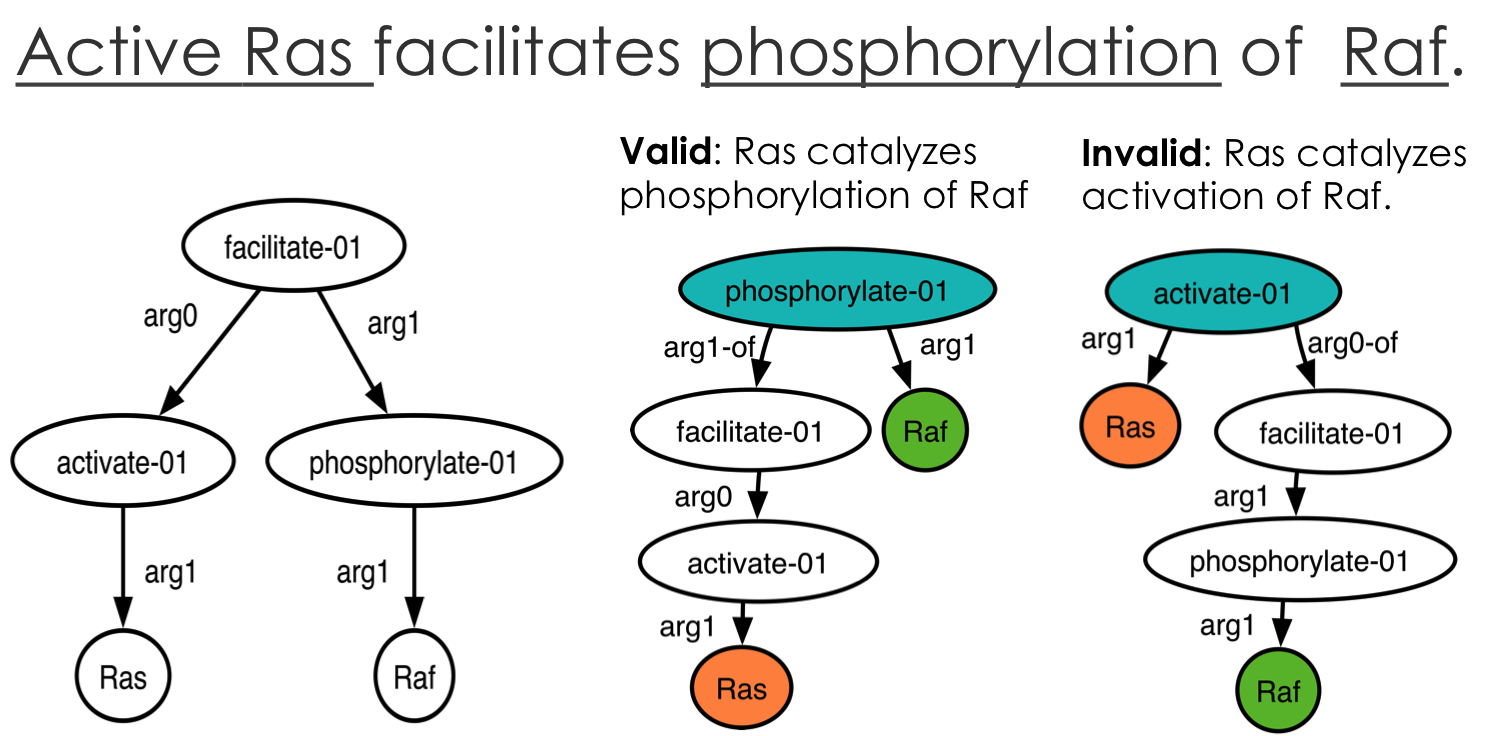
Figure 1: On the left, we show an abstract meaning representation (AMR) of a sentence. As per the semantics of the sentence, there is a valid biomedical relationship between the two proteins, Ras and Raf, i.e. Ras catalyzes phosphorylation of Raf; the relation corresponds to a subgraph extracted from the AMR. On the other hand, one of the many invalid biomedical relationships that one could infer is, Ras catalyzes activation of Raf, for which we show the corresponding subgraph too. A given candidate relation automatically hypothesized from the sentence, is binary classified, as valid or invalid, using the subgraph as features.

In a very recent work, kernelized locality sensitive hashcodes based representation learning approach has been proposed that has shown to be the most successful in terms of accuracy and computational efficiency for the task Garg et al. (2019). The model parameters, shared between all the hash functions, are optimized in a supervised manner, whereas an individual hash function is constructed in a randomized fashion. The authors suggest to obtain thousands of (randomized) semantic features extracted from natural language data points into binary hashcodes, and then making classification decision as per the features using hundreds of decision trees, which is the core of their robust classification approach. Even if we extract thousands of semantic features using the hashing approach, it is difficult to ensure that the features extracted from training data points would generalize to a test set. While the inherent randomness in constructing hash functions from a training set can help towards generalization in the case of absence of a test set, there should be better alternatives if we do have the knowledge of a test set of data points, or a subset of a training set treated as a pseudo-test set. What if we construct hash functions in an intelligent manner via exploiting the additional knowledge of unlabeled data points in a test/pseudo-test set, performing fine-grained optimization of each hash function rather than relying upon randomness, so as to extract semantic features which generalize?

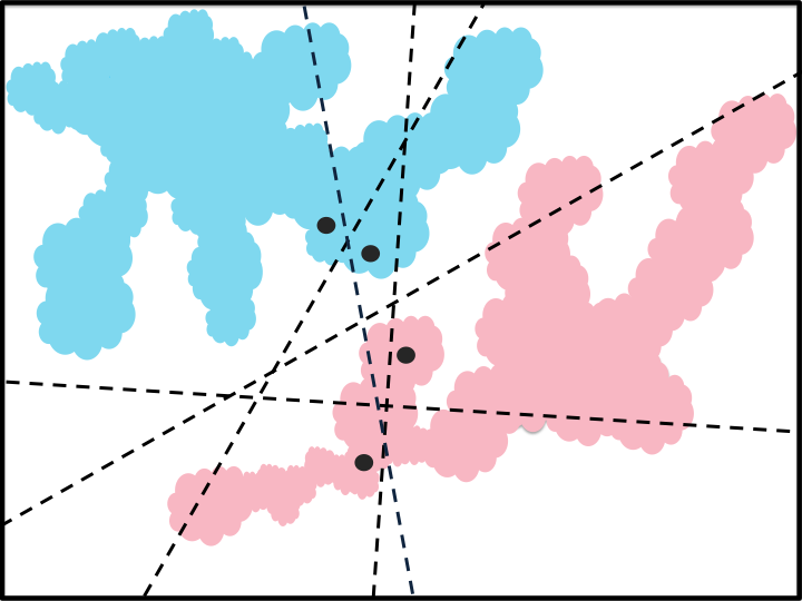
(a) Hash function choices

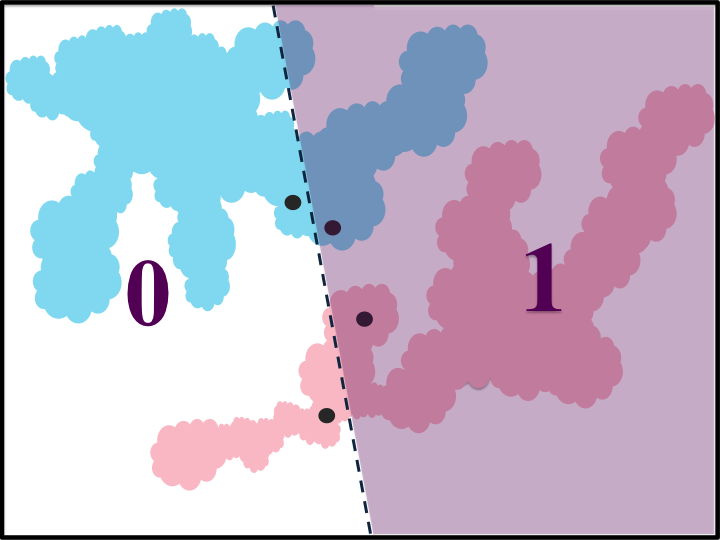
(b) Generalizing hash function

Figure 2: In this figure, we illustrate how to construct hash functions which generalize across a training and a test set. Blue and red colors denote training and test data points respectively. A hash function is constructed by splitting a very small subset of data points into two parts. In Fig. 2(a), given the set of four data points selected randomly, there are many choices possible for splitting the set, corresponding to difference choices of hash functions which are denoted with dashed lines. The optimal choice of hash function is shown in Fig. 2(b) since it generalizes well, assigning same value to many data points from both training & test sets.

Along these lines, we propose a new framework for learning hashcode representations accomplishing two important (inter-related) extensions w.r.t. the previous work:

(a) We propose to use a nearly unsupervised hashcode representation learning setting, in which we use only the knowledge of which set a data point comes from, a training set or a test/pseudo-test set, along with the data point itself, whereas the actual class labels of data points from a training set are input only to the final supervised-classifier, such as a Random Forest, which takes input of the learned hashcodes as representation (feature) vectors of data points along with their class labels;

(b) We introduce multiple concepts for fine-grained (discrete) optimization of hash functions, employed in our novel information-theoretic algorithm that constructs hash functions greedily one by one. In supervised settings, fine-grained (greedy) optimization of hash functions could lead to overfitting whereas, in our proposed nearly-unsupervised framework, it allows flexibility for explicitly maximizing the generalization capabilities of hash functions.

For a task of biomedical relation extraction, we evaluate our approach on four public datasets, and obtain significant gains in F1 scores w.r.t. state-of-the-art models including kernel-based approaches as well the ones based on semi-supervised learning of neural networks. We also show how to employ our framework for learning locality sensitive hashcode representations using neural networks.

2 Problem Formulation & Background

In Fig. 1, we demonstrate how biomedical relations between entities are extracted from the semantic (or syntactic) parse of a sentence. As we see, the task is formulated as of binary classification of natural language sub-structures extracted from the semantic parse. Suppose we have natural language structures, $\boldsymbol{S}=\{S_{i}\}_{1}^{N}$, such as parse trees, shortest paths, text sentences, etc, with corresponding class labels, $\boldsymbol{y}=\{y_{i}\}_{1}^{N}$. For the data points coming from a training set and a test set, we use notations, $\boldsymbol{S}_{T}$, and $\boldsymbol{S}_{*}$, respectively; same applies for the class labels. In addition, we define indicator variable, $\boldsymbol{x}=\{x_{i}\}_{i=1}^{N}$, for $\boldsymbol{S}$, with $x_{i}\in\{0,1\}$ denoting if a data point $S_{i}$ is coming from a test/pseudo-test set or a training set. Our goal is to infer the class labels of the data points from a test set, $\boldsymbol{y}_{*}$.

2.1 Hashcode Representations

As per the hashcode representation approach, $\boldsymbol{S}$ is mapped to a set of locality sensitive hashcodes, $\boldsymbol{C}=\{\boldsymbol{c}_{i}\}_{1}^{N}$, using a set of $H$ binary hash functions, i.e. $\boldsymbol{c}_{i}=\boldsymbol{h}(S_{i})=\{h_{1}(S_{i}),\cdots,h_{H}(S_{i})\}$. $h_{l}(.;\boldsymbol{\theta})$ is constructed such that it splits a set of data points, $\boldsymbol{S}^{R}_{l}$, into two subsets as shown in Fig. 2(a), while choosing the set as a small random subset of size $\alpha$ from the superset $\boldsymbol{S}$, i.e. $\boldsymbol{S}^{R}_{l}\subset\boldsymbol{S}$ s.t. $|\boldsymbol{S}^{R}_{l}|=\alpha\ll N$. In this manner, we can construct a large number of hash functions, $\{h_{l}(.;\boldsymbol{\theta})\}_{l=1}^{H}$, from a reference set of size $M$, $\boldsymbol{S}^{R}=\{\boldsymbol{S}^{R}_{1}\cup\cdots\cup\boldsymbol{S}^{R}_{H}\},|\boldsymbol{S}^{R}|=M\leq\alpha H\ll N$.

While, mathematically, a locality sensitive hash function can be of any form, kernelized hash functions Garg et al. (2019, 2018); Joly and Buisson (2011), rely upon a convolution kernel similarity function $K(S_{i},S_{j};\boldsymbol{\theta})$ defined for any pair of structures $S_{i}$ and $S_{j}$ with kernel-parameters $\boldsymbol{\theta}$ Haussler (1999). To construct $h_{l}(.)$, a kernel-trick based model, such as kNN, SVM, is fit to $\{\boldsymbol{S}^{R}_{l},\boldsymbol{z}_{l}\}$, with a randomly sampled binary vector, $\boldsymbol{z}_{l}\in\{0,1\}^{\alpha}$, that defines the split of $\boldsymbol{S}^{R}_{l}$. For computing hashcode $\boldsymbol{c}_{i}$ for $S_{i}$, it requires only $M$ number of convolution-kernel similarities of $S_{i}$ w.r.t. the data points in $\boldsymbol{S}^{R}$, which makes this approach highly scalable in compute cost terms.

In the previous work Garg et al. (2019), it is proposed to optimize all the hash functions jointly by learning only the parameters which are shared amongst all the functions, i.e. learning kernel parameters, $\boldsymbol{\theta}$ and the choice of reference set, $\boldsymbol{S}^{R}\subset\boldsymbol{S}_{T}$. This optimization is performed in a supervised manner via maximization of the mutual information between hashcodes of data points and their class labels, using $\{\boldsymbol{S}_{T},\boldsymbol{y}_{T}\}$ for training.

3 Nearly-Unsupervised Hashcode Representations

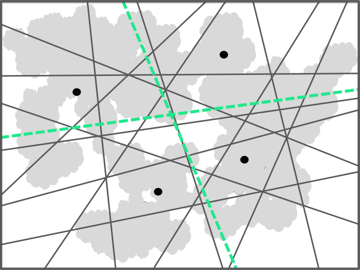
(a) Global sampling

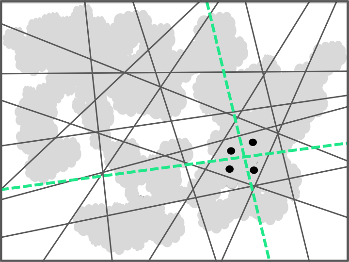
(b) Local sampling from a cluster

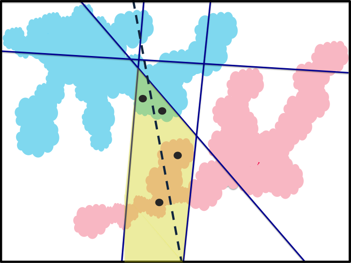
(c) Local sampling from a high-entropy cluster

Figure 3: In all the three figures, dark-gray lines denote hash functions optimized previously, and intersections of the lines give us 2-D cells denoting hashcodes as well as clusters; black dots represent a set of data points which are used to construct a hash function, and some of the choices to split the subset are shown as green dashed lines. The procedure of sampling the subset varies across the three figures. In Fig. 3(a), since the four data points from global sampling have already unique hashcodes (2-D cells), the newly constructed hash function (one of the green dashed-lines) adds little information to their representations. On the other hand in Fig. 3(b), a hash function constructed from a set of data points, which are sampled locally from within a cluster, puts some of the data points in the sampled set into two different cells (hashcodes), so adding more fine-grained information to their representations, hence more advantageous from representation learning perspective. In Fig. 3(c), training and test data points are denoted with blue and red colors respectively, and the data points to construct a new hash function are sampled locally from within a high entropy cluster, i.e. the one containing a balanced proportion of the training & test data points.

Our key insight in regards to limitation of the previous approach for supervised learning of hashcode representations, is that, to avoid overfitting, learning is intentionally restricted only to the optimization of shared parameters whereas each hash function $h_{l}(.)$ is constructed in a randomized manner, i.e. random sub-sampling of a subset, $\boldsymbol{S}^{R}_{l}\subset\boldsymbol{S}$, and a random split of the subset. On the other hand, in a nearly-unsupervised hashcode learning settings as we introduce next, we can have the additional knowledge of data points from a test/pseudo-test set which can be leveraged to extend the optimization from the shared (global) parameters to fine-grained optimization of hash functions, not only to avoid overfitting but for higher generalization of hashcodes across training & test sets.

Nearly unsupervised learning settings

We propose to learn hash functions, $\boldsymbol{h}(.)$, using $\boldsymbol{S}=\{\boldsymbol{S}_{T},\boldsymbol{S}_{*}\}$, $\boldsymbol{x}$, and optionally, $\boldsymbol{y}_{T}$. Herein, $\boldsymbol{S}_{*}$ is a test set, or a pseudo-test set that can be a random subset of the training set or a large set of unlabeled data points outside the training set.

3.1 Basic Concepts for Fine-Grained Optimization

In the prior works on kernel-similarity based locality sensitive hashing, the first step for constructing a hash function is to randomly sample a small subset of data points, from a superset $\boldsymbol{S}$, and in the second step, the subset is split into two parts using a kernel-trick based model Garg et al. (2019, 2018); Joly and Buisson (2011), serving as the hash function, as described in Sec. 2.

In the following, we introduce basic concepts for improving upon these two key aspects of constructing a hash function, while later, in Sec. 3.2, these concepts are incorporated in a unified manner in our proposed information-theoretic algorithm that greedily optimizes hash functions one by one.

Informative split

In Fig. 2(a), construction of a hash function is pictorially illustrated, showing multiple possible splits, as dotted lines, of a small set of four data points (black dots). (Note that a hash function is shown to be a linear hyperplane only for simplistic explanations of the basic concepts.) While in the previous works, one of the many choices for splitting the set is chosen randomly, we propose to optimize upon this choice. Intuitively, one should choose a split of the set, corresponding to a hash function, such that it gives a balanced split for the whole set of data points, and it should also generalize across training & test sets. In reference to the figure, one simple way to analyze the generalization of a split (so the hash function) is to see if there are training as well as test data points (or pseudo-test data points) on either side of the dotted line. As per this concept, an optimal split of the set of four data points is shown in Fig. 2(b).

Referring back to Sec. 2, clearly, this is a combinatorial optimization problem, where we need to choose an optimal choice of $\boldsymbol{z}_{l}\in\{0,1\}^{\alpha}$ for set, $\boldsymbol{S}^{R}_{l}$, to construct $h_{l}(.)$. For a small value of $\alpha$, one can either go through all the possible combinations in a brute force manner, or use Markov Chain Monte Carlo sampling. It is interesting to note that, even though a hash function is constructed from a very small set of data points (of size $\alpha\not\gg 1$), the generalization criterion, formulated in our info-theoretic objective introduced in Sec. 3.2, is computed using all the data points available for the optimization, $\boldsymbol{S}$.

Local sampling from a cluster

Another aspect of constructing a hash function, having a scope for improvement, is sampling of a small subset of data points, $\boldsymbol{S}^{R}_{l}\subset\boldsymbol{S}$, that is used to construct a hash function. In the prior works, the selection of such a subset is purely random, i.e. random selection of data points globally from $\boldsymbol{S}$. In Fig. 3, we illustrate that, it is wiser to (randomly) select data points locally from one of the clusters of the data points in $\boldsymbol{S}$, rather than sampling globally from $\boldsymbol{S}$. Here, we propose that clustering of all the data points in $\boldsymbol{S}$ can be obtained using the hash functions itself, due to their locality sensitive property. While using a large number of locality sensitive hash functions give us fine-grained representations of data points, a small subset of the hash functions, of size $\zeta$, defines a valid clustering of the data points, since data points which are similar to each other should have same hashcodes serving as cluster labels.

From this perspective, we can construct first few hash functions from global sampling of data points, what we refer as global hash functions. These global hash functions should serve to provide hashcode representations as well as clusters of data points. Then, via local sampling from the clusters, we can also construct local hash functions to capture more finer details of data points. As per this concept, we can learn hierarchical (multi-scale) hashcode representations of data points, capturing differences between data points from coarser (global hash functions) to finer scales (local hash functions).

Further, we suggest to choose a cluster that has a balanced proportion of training & test (pseudo-test) data points, which is desirable from the perspective of having generalized hashcode representations; see Fig. 3(c).

Splitting other clusters

In reference to Fig. 4, non-redundancy of a hash function w.r.t. the other hash functions can be characterized in terms of how well the hash function splits the clusters defined as per the other hash functions.

Next we mathematically formalize all the concepts introduced above for fine-grained optimization of hash functions into an information-theoretic objective function.

3.2 Information-Theoretic Learning

Algorithm 1 Nearly-Unsupervised Hashcode Representation Learning

0:  Dataset $\{\boldsymbol{S},\boldsymbol{x}\}$, and parameters, $H,\boldsymbol{\alpha},\zeta$.

1:  $\boldsymbol{h}(.)\leftarrow\{\}$, $\boldsymbol{C}\leftarrow\{\}$, $\boldsymbol{f}\leftarrow\{\}$ %Greedy step for optimizing hash function, $h_{l}(.)$

2:  while $|\boldsymbol{h}(.)|<H$ do

3:     $\alpha_{l}\leftarrow$ sampleSubsetSize$\left(\boldsymbol{\alpha}\right)$ %Sample a size for the subset of data points, $\boldsymbol{S}^{R}_{l}$, to construct a hash function

4:     if $|\boldsymbol{h}(.)|<\zeta$ then

5:        $\boldsymbol{S}^{R}_{l}\leftarrow$ randomSampleGlobally$\left(\boldsymbol{S},\alpha_{l}\right)$ %Randomly sample data points, globally from $\boldsymbol{S}$, for constructing a global hash function.

6:     else 7:        $\boldsymbol{S}^{R}_{l}\leftarrow$ randomSampleLocally$\left(\boldsymbol{S},\boldsymbol{C},\boldsymbol{x},\alpha_{l},\zeta\right)$ %Sample data points randomly from, a high entropy cluster, for constructing a local hash function.

8:     end if 9:     $h_{l}(.),f_{l}\!\leftarrow\!$ optimizeSplit$\left(\boldsymbol{S}^{R}_{l},\boldsymbol{S},\boldsymbol{C},\boldsymbol{x}\right)$ %Optimize split of $\boldsymbol{S}^{R}_{l}$.

10:     $\boldsymbol{c}\leftarrow$ computeHash$\left(\boldsymbol{S},h_{l}(.)\right)$

11:     $\boldsymbol{C}\leftarrow\boldsymbol{C}\cup\boldsymbol{c}$, $\boldsymbol{h}(.)\leftarrow\boldsymbol{h(.)}\cup h_{l}(.)$, $\boldsymbol{f}\leftarrow\boldsymbol{f}\cup f_{l}$.

12:     $\boldsymbol{h}(.),\boldsymbol{C},\boldsymbol{f}\leftarrow$ deleteLowInfoFunc$\left(\boldsymbol{h}(.),\boldsymbol{C},\boldsymbol{f}\right)$ %delete hash functions from the set with lower objective values

13:  end while

14:  Return $\boldsymbol{h}(.),\boldsymbol{C}$.

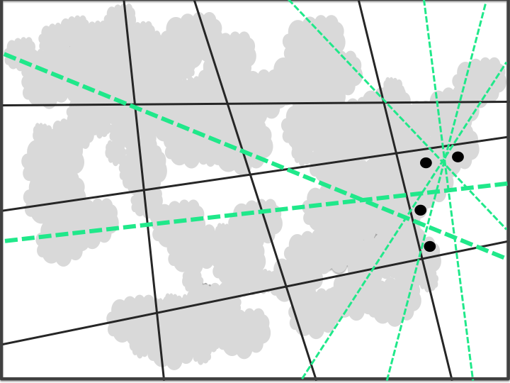
Figure 4: Dark-gray lines denote hash functions optimized previously, and gray color represents data points used for the optimization. The intersections of the lines give us 2-D cells, corresponding to hashcodes as well as clusters. For the set of four data points sampled within a cluster, there are many choices to split it (corresponding to hash functions choices), shown with dashed lines. We propose to choose the one which also splits the sets of data points in other (neighboring) clusters in a balanced manner, i.e. having data points in a cluster on either side of the dashed line and cutting through as many clusters as possible. As per this criterion, the thick-green dashed lines are superior choices w.r.t. the thin-green ones.

We optimize hash functions greedily, one by one. Referring back to Sec. 2, we define binary random variable $x$ denoting if a data point comes from a training set or a test/pseudo-test set. In a greedy step of optimizing a hash function, random variable, $\boldsymbol{c}$, represents the hashcode of a data point $S$, as per the previously optimized hash functions $\boldsymbol{h}_{l-1}(.)$. Along same lines, $c$ denotes the binary random variable corresponding from the present hash function under optimization, $h_{l}(.)$. We maximize the information-theoretic objective as below.

$$\arg\!\max_{h_{l}()}{\mathcal{H}}(x,c)-{\mathcal{I}}(c:\boldsymbol{c})+{\mathcal{H}}(x|\boldsymbol{c});$$ (1)

$$\boldsymbol{c}=\boldsymbol{h}_{l-1}(S),c=h_{l}(S)$$

Herein the optimization of a hash function, $h_{(}.)$, involves intelligent selection of $\boldsymbol{S}^{R}_{l}$, an informative split of $\boldsymbol{S}^{R}_{l}$, i.e. optimizing $\boldsymbol{z}_{l}$ for $\boldsymbol{S}^{R}_{l}$, and learning of the parameters $\boldsymbol{\theta}$ of a (kernel or neural) model, which is fit on $\{\boldsymbol{S}^{R}_{l},\boldsymbol{z}_{l}\}$, acting as the hash function.

In the objective function above, maximizing the first term, ${\mathcal{H}}(x,c)$, i.e. joint entropy on $x$ and $c$, corresponds to the concept of informative split described above in Sec. 3.1; see Fig. 2. This term is cheap to compute since $x$ and $c$ are both 1-dimensional binary variables.

The second term in the objective, the mutual information term, ensures minimal redundancies between hash functions. This is related to the concept of constructing a hash function such that it splits many of the existing clusters, as mentioned above in Sec. 3.1; see Fig. 4. This mutual information function can be computed using the approximation in the previous work by  Garg et al. (2019).

The last quantity in the objective is ${\mathcal{H}}(x|\boldsymbol{c})$, conditional entropy on $x$ given $\boldsymbol{c}$. We propose to maximize this term indirectly via choosing a cluster informatively, from which to randomly select data points for constructing the hash function, such that it contains a balanced ratio of the count of training & test data points, i.e. a cluster with high entropy on $x$, which we refer as a high entropy cluster. In reference to Fig. 3(c), the new clusters emerging from a split of a high entropy cluster should have higher chances to be high entropy clusters themselves, thus maximizing the last term indirectly. We compute marginal entropy on $x$ for each cluster, and an explicit computation of $H(x|\boldsymbol{c})$ is not required.

Optionally one may extend the objective to include the term, $-{\mathcal{H}}(y|\boldsymbol{c},c)$, with $y$ denoting the random variable for a class label.

The above described learning framework is summarized in Alg. 1.

Besides kernelized locality sensitive hashcodes, the above framework allows neural locality sensitive hashing. One can fit any  (regularized) neural model on $\{\boldsymbol{S}^{R}_{l},\boldsymbol{z}_{l}\}$, acting as a neural locality sensitive hash function. We expect that some of the many possible choices for a split of $\boldsymbol{S}^{R}_{l}$ should lead to natural semantic categorizations of the data points. For such a natural split choice, even a parameterized model can act as a good hash function without overfitting as we observed empirically.

In the algorithm, we also propose to delete some of the hash functions from the set of optimized ones, the ones which have low objective function values w.r.t. the rest. This step provides robustness against an arbitrarily bad choice of randomly selected subset, $\boldsymbol{S}^{R}_{l}$.

Our algorithm allows parallel computing, as in the previous hashcode learning approach.

4 Experiments

We demonstrate the applicability of our approach for a challenging task of biomedical relation extraction, using four public datasets.

Dataset details

For AIMed and BioInfer, cross-corpus evaluations have been performed in many previous works Airola et al. (2008); Tikk et al. (2010); Peng and Lu (2017); Hsieh et al. (2017); Rios et al. (2018); Garg et al. (2019). These datasets have annotations on pairs of interacting proteins (PPI) in a sentence while ignoring the interaction type. Following the previous works, for a given pair of proteins mentioned in a text sentence from a training or a test set, we obtain the corresponding undirected shortest path from a Stanford dependency parse of the sentence, that serves as a data point.

We also use PubMed45 and BioNLP datasets which have been used for extensive evaluations in recent works Garg et al. (2019, 2018); Rao et al. (2017); Garg et al. (2016). These two datasets consider a relatively more difficult task of inferring an interaction between two or more bio-entities mentioned in a sentence, along with the inference of their interaction-roles, and the type of interaction from an unrestricted list. As in the previous works, we use abstract meaning representation (AMR) to obtain shortest path-based data points Banarescu et al. (2013); same bio-AMR parser Pust et al. (2015) is employed as in the previous works. PubMed45 dataset has 11 subsets, with evaluation performed for each of the subsets as a test set leaving the rest for training (not to be confused with cross-validation). For BioNLP dataset Kim et al. (2009, 2011); Nédellec et al. (2013), the training set contains annotations from years 2009, 2011, 2013, and the test set contains development set from year 2013. Overall, for a fair comparison of the models, we keep same experimental setup as followed in Garg et al. (2019), for all the four datasets, so as to avoid any bias due to engineering aspects; evaluation metrics for the relation extraction task are, f1 score, precision, recall.

Baseline methods

The most important baseline method for the comparison is the recent work of supervised hashcode representations Garg et al. (2019). Their model is called as KLSH-RF, with KLSH referring to kernelized locality sensitive hashcodes, and RF denotes Random Forest. Our approach differs from their work in the sense that our hashcode representations are nearly unsupervised, whereas their approach is purely supervised, while both approaches use a supervised RF. We refer to our model as KLSH-NU-RF. Within the nearly unsupervised learning setting, we consider transductive setting by default, i.e. using data points from both training and test sets. Later, we also show results for inductive settings, i.e. using a random subset of training data points, as a pseudo-test set. In both scenarios, we do not use class labels for learning hashcodes, but only for training RF.

Models	(A, B)	(B, A)
SVM (Airola08)	0.47	0.47
SVM (Miwa09)	0.53	0.50
SVM (Tikk10)	0.41	0.42
	(0.67, 0.29)	(0.27, 0.87)
CNN (Nguyen15)	0.37	0.45
Bi-LSTM (Kavuluru17)	0.30	0.47
CNN (Peng17)	0.48	0.50
	(0.40, 0.61)	(0.40, 0.66)
RNN (Hsieh17)	0.49	0.51
CNN-RevGrad (Ganin16)	0.43	0.47
Bi-LSTM-RevGrad (Ganin16)	0.40	0.46
Adv-CNN (Rios18)	0.54	0.49
Adv-Bi-LSTM (Rios18)	$\boldsymbol{0.57}$	0.49
KLSH-kNN (Garg18)	$0.51$	$0.51$
	(0.41, 0.68)	(0.38, 0.80)
KLSH-RF (Garg19)	$\boldsymbol{0.57}$	$0.54$
	(0.46, 0.75)	(0.37, 0.95)
SSL-VAE (Zhang19)	0.50	0.46
	(0.38, 0.72)	(0.39, 0.57)
KLSH-NU-RF	$\boldsymbol{0.57}$	$\boldsymbol{0.57}$
	(0.44, 0.81)	(0.44, 0.81)

Table 1: Evaluation results from cross-corpus evaluation for (train, test) pairs of datasets, AIMed (A) and BioInfer (B). For each model, we report F1 score, and if available, precision, recall scores are also shown in brackets. For the adversarial neural models by Ganin et al. (2016), evaluation on the datasets was provided by Rios et al. (2018).

For AIMed and BioInfer datasets, adversarial learning based four neural network models had been evaluated in the prior works Rios et al. (2018); Ganin et al. (2016), referred as CNN-RevGrad, Bi-LSTM-RevGrad, Adv-CNN, Adv-CNN. Like our model KLSH-NU-RF, these four models are also learned in transductive settings of using data points from the test set in addition to the training set. Semi-supervised Variational Autoencoders (SSL-VAE) have also been explored for biomedical relation extraction Zhang and Lu (2019), which we evaluate ourselves for all the four datasets considered in this paper.

Parameter settings

We use path kernels with word vectors & kernel parameter settings as in the previous work Garg et al. (2019). From a preliminary tuning, we set the number of hash functions, $H=100$, and the number of decision trees in a Random Forest classifier, $R=100$; these parameters are not sensitive, requiring minimal tuning. For any other parameters which may require fine-grained tuning, we use 10% of training data points, selected randomly, for validation. Within kernel locality sensitive hashing, we choose between Random Maximum Margin and Random k-Nearest Neighbors techniques, and for neural locality sensitive hashing, we use a simple 2-layer LSTM model with 8 units per layer. In our nearly unsupervised learning framework, we use subsets of the hash functions, of size 10, to obtain clusters ($\zeta=10$). We employ 8 cores on an i7 processor, with 32GB memory, for all the computations.

Models	PubMed45	BioNLP
SVM (Garg16)	$0.45$$\pm$$0.25$	$0.46$
	(0.58, 0.43)	(0.35, 0.67)
LSTM (Rao17)	N.A.	0.46
		(0.51, 0.44)
LSTM (Garg19)	$0.30$$\pm$$0.21$	0.59
	(0.38, 0.28)	(0.89, 0.44)
Bi-LSTM (Garg19)	$0.46$$\pm$$0.26$	0.55
	(0.59, 0.43)	(0.92, 0.39)
LSTM-CNN (Garg19)	$0.50$$\pm$$0.27$	0.60
	(0.55, 0.50)	(0.77, 0.49)
CNN (Garg19)	$0.51$$\pm$$0.28$	0.60
	(0.46, 0.46)	(0.80, 0.48)
KLSH-kNN (Garg18)	$0.46$$\pm$$0.21$	$0.60$
	(0.44, 0.53)	(0.63, 0.57)
KLSH-RF (Garg19)	$0.57$$\pm$$0.25$	$0.63$
	(0.63, 0.55)	(0.78, 0.53)
SSL-VAE (Zhang19)	$0.40\pm 0.16$	$0.48$
	(0.33, 0.69)	(0.43, 0.56)
KLSH-NU-RF	$\boldsymbol{0.61}$$\pm$$\boldsymbol{0.23}$	$\boldsymbol{0.67}$
	(0.61, 0.62)	(0.73, 0.61)

Table 2: Evaluation results for PubMed45 and BioNLP datasets. We report F1 score (mean $\pm$ standard deviation), and mean-precision & mean-recall numbers in brackets. For BioNLP, we standard deviation numbers are not provided as there is one fixed test subset.

4.1 Experimental Results

In summary, our model KLSH-NU-RF significantly outperforms its purely supervised counterpart, KLSH-RF, and also semi-supervised neural network models.

In reference to Tab. 1, we first discuss results for the evaluation setting of using AIMed dataset as a test set, and BioInfer as a training set. We observe that our model, KLSH-NU-RF, obtains F1 score, 3 pts higher w.r.t. the most recent baseline, KLSH-RF. In comparison to the semi-supervised neural neural models, CNN-RevGrad, Bi-LSTM-RevGrad, Adv-CNN, Adv-Bi-LSTM, SSL-VAE, which use the knowledge of a test set just like our model, we gain 8-11 pts in F1 score. On the other hand, when evaluating on BioInfer dataset as a test set and AIMed as a training set, our model is in tie w.r.t. the adversarial neural model, Adv-Bi-LSTM, though outperforming the other three adversarial models and SSL-VAE, by large margins in F1 score. In comparison to KLSH-RF, we retain same F1 score, while gaining in recall by 6 pts at the cost of losing 2 pts in precision.

For PubMed and BioNLP datasets, there is no prior evaluation of adversarial models. Nevertheless, in Tab. 2, we see that our model significantly outperforms SSL-VAE, and it also outperforms the most relevant baseline, KLSH-RF, gaining F1 score by 4 pts for both the datasets. Note that, high standard deviations reported for PubMed45 dataset are due to high diversity across the 11 test sets, while the performance of our model for a given test set is highly stable (improvements are statistically significant with p-value: 6e-3).

One general trend to observe is that the proposed nearly unsupervised learning approach leads to a significantly higher recall, at the cost of marginal drop in precision, w.r.t. its supervised baseline.

Figure 5: Comparison across the three types of learning settings, supervised, transductive, and inductive.

Further, note that the number of hash functions used in the prior work is 1000 whereas we use only 100 hash functions. Compute time is same as for their model.

Our approach is easily extensible for other modeling aspects such as non-stationary kernel functions, document level inference, joint use of semantic & syntactic parses, ontology or database usage Garg et al. (2019, 2016); Alicante et al. (2016), though we refrain from presenting system level evaluations, and have focused only upon analyzing improvements from our principled extension of the recently proposed technique that has already been shown to be successful for the task.

Transductive vs inductive settings

In the above discussed results, hashcode representations in our models are learned in transductive setting. For inductive settings, we randomly select 25% of the training data points for use as a pseudo-test set instead of the test set. In Fig. 5, we observe that both inductive and transductive settings are more favorable w.r.t. the supervised one, KLSH-RF, which is the baseline in this paper. F1 scores obtained from the inductive setting are on a par with the transductive settings. It is worth noting that, in inductive settings, our model is trained on information even lesser than the baseline model KLSH-RF, yet it obtains F1 scores significantly higher.

Neural hashing

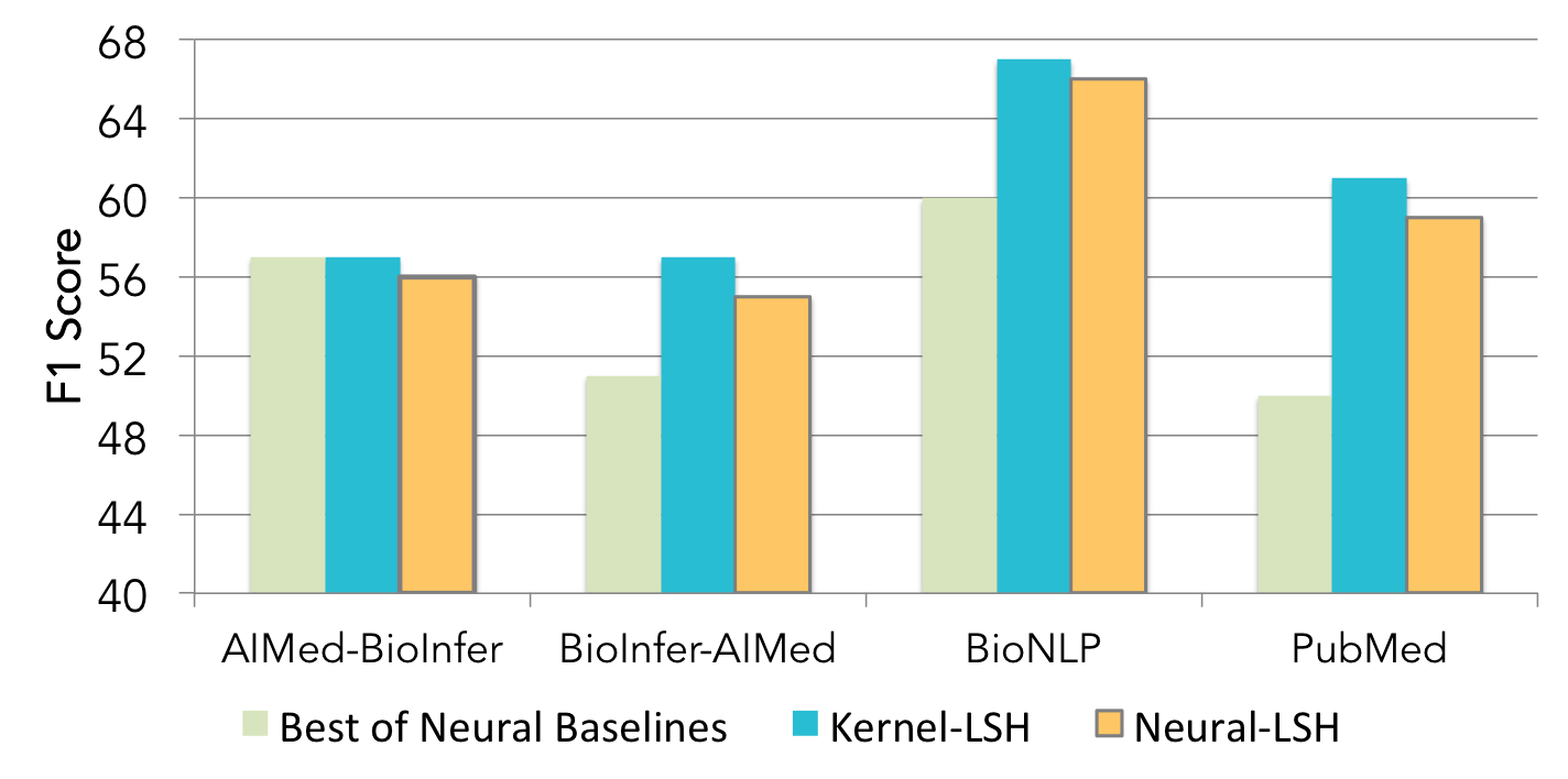
Figure 6: Comparison of neural hashing w.r.t. kernel hashing, and the best of neural baselines.

In Fig. 6, we show results for neural locality sensitive hashing within our proposed framework, and observe that neural hashing is a little worse than its kernel based counterpart, however it performs significantly superior w.r.t. the best of other neural models.

5 Conclusions

We proposed a nearly-unsupervised framework for learning of kernelized locality sensitive hashcode representations, a recent technique, that was originally supervised, which has shown state-of-the-art results for a difficult task of biomedical relation extraction. Within our proposed framework, we use the additional knowledge of test/pseudo-test data points for fine-grained optimization of hash functions so as to obtain hashcode representations generalizing across training & test sets. Our experiment results show significant improvements in accuracy numbers w.r.t. the supervised baseline, as well as semi-supervised neural network models, for the same task of bio-medical relation extraction across four public datasets.

6 Acknowledgments

This work was sponsored by the DARPA Big Mechanism program (W911NF-14-1-0364). It is our pleasure to acknowledge fruitful discussions with Shushan Arakelyan, Amit Dhurandhar, Sarik Ghazarian, Palash Goyal, Karen Hambardzumyan, Hrant Khachatrian, Kevin Knight, Daniel Marcu, Dan Moyer, Kyle Reing, and Irina Rish. We are also grateful to anonymous reviewers for their valuable feedback.

References

- Airola et al. (2008) Antti Airola, Sampo Pyysalo, Jari Björne, Tapio Pahikkala, Filip Ginter, and Tapio Salakoski. 2008. All-paths graph kernel for protein-protein interaction extraction with evaluation of cross-corpus learning. BMC Bioinformatics.
- Alicante et al. (2016) Anita Alicante, Massimo Benerecetti, Anna Corazza, and Stefano Silvestri. 2016. A distributed architecture to integrate ontological knowledge into information extraction. International Journal of Grid and Utility Computing.
- Banarescu et al. (2013) Laura Banarescu, Claire Bonial, Shu Cai, Madalina Georgescu, Kira Griffitt, Ulf Hermjakob, Kevin Knight, Philipp Koehn, Martha Palmer, and Nathan Schneider. 2013. Abstract meaning representation for sembanking. In Proceedings of the Linguistic Annotation Workshop and Interoperability with Discourse.
- Chang et al. (2016) Yung-Chun Chang, Chun-Han Chu, Yu-Chen Su, Chien Chin Chen, and Wen-Lian Hsu. 2016. PIPE: a protein–protein interaction passage extraction module for biocreative challenge. Database.
- Cohen (2015) Paul R Cohen. 2015. DARPA’s big mechanism program. Physical biology.
- Ganin et al. (2016) Yaroslav Ganin, Evgeniya Ustinova, Hana Ajakan, Pascal Germain, Hugo Larochelle, Francois Laviolette, Mario Marchand, and Victor Lempitsky. 2016. Domain-adversarial training of neural networks. Journal of Machine Learning.
- Garg et al. (2016) Sahil Garg, Aram Galstyan, Ulf Hermjakob, and Daniel Marcu. 2016. Extracting biomolecular interactions using semantic parsing of biomedical text. In Proceedings of the AAAI Conference on Artificial Intelligence.
- Garg et al. (2019) Sahil Garg, Aram Galstyan, Greg Ver Steeg, Irina Rish, Guillermo Cecchi, and Shuyang Gao. 2019. Kernelized hashcode representations for relation extraction. In Proceedings of the AAAI Conference on Artificial Intelligence.
- Garg et al. (2018) Sahil Garg, Greg Ver Steeg, and Aram Galstyan. 2018. Stochastic learning of nonstationary kernels for natural language modeling. arXiv preprint arXiv:1801.03911.
- Hahn and Surdeanu (2015) Marco A Valenzuela-Escárcega Gus Hahn and Powell Thomas Hicks Mihai Surdeanu. 2015. A domain-independent rule-based framework for event extraction. In Proceedings of ACL-IJCNLP.
- Haussler (1999) David Haussler. 1999. Convolution kernels on discrete structures. Technical report.
- Hsieh et al. (2017) Yu-Lun Hsieh, Yung-Chun Chang, Nai-Wen Chang, and Wen-Lian Hsu. 2017. Identifying protein-protein interactions in biomedical literature using recurrent neural networks with long short-term memory. In Proceedings of the International Joint Conference on Natural Language Processing.
- Joly and Buisson (2011) Alexis Joly and Olivier Buisson. 2011. Random maximum margin hashing. In Proceedings of the Conference on Computer Vision and Pattern Recognition.
- Kavuluru et al. (2017) Ramakanth Kavuluru, Anthony Rios, and Tung Tran. 2017. Extracting drug-drug interactions with word and character-level recurrent neural networks. In IEEE International Conference on Healthcare Informatics.
- Kim et al. (2009) Jin-Dong Kim, Tomoko Ohta, Sampo Pyysalo, Yoshinobu Kano, and Jun’ichi Tsujii. 2009. Overview of BioNLP’09 shared task on event extraction. In Proceedings of the Workshop on Current Trends in Biomedical Natural Language Processing: Shared Task.
- Kim et al. (2011) Jin-Dong Kim, Sampo Pyysalo, Tomoko Ohta, Robert Bossy, Ngan Nguyen, and Jun’ichi Tsujii. 2011. Overview of BioNLP shared task 2011. In Proceedings of the BioNLP Shared Task Workshop.
- Kingma et al. (2014) Durk P Kingma, Shakir Mohamed, Danilo Jimenez Rezende, and Max Welling. 2014. Semi-supervised learning with deep generative models. In Proceedings of the Neural Information Processing Systems Conference.
- Miwa et al. (2009) Makoto Miwa, Rune Sætre, Yusuke Miyao, and Jun’ichi Tsujii. 2009. Protein–protein interaction extraction by leveraging multiple kernels and parsers. International Journal of Medical Informatics.
- Mooney and Bunescu (2005) Raymond J Mooney and Razvan C Bunescu. 2005. Subsequence kernels for relation extraction. In Proceedings of the Neural Information Processing Systems Conference.
- Nédellec et al. (2013) Claire Nédellec, Robert Bossy, Jin-Dong Kim, Jung-Jae Kim, Tomoko Ohta, Sampo Pyysalo, and Pierre Zweigenbaum. 2013. Overview of BioNLP shared task 2013. In Proceedings of the BioNLP Shared Task Workshop.
- Nguyen and Grishman (2015) Thien Huu Nguyen and Ralph Grishman. 2015. Relation extraction: Perspective from convolutional neural networks. In Proceedings of the 1st Workshop on Vector Space Modeling for Natural Language Processing.
- Peng and Lu (2017) Yifan Peng and Zhiyong Lu. 2017. Deep learning for extracting protein-protein interactions from biomedical literature. In Proceedings of BioNLP Workshop.
- Pust et al. (2015) Michael Pust, Ulf Hermjakob, Kevin Knight, Daniel Marcu, and Jonathan May. 2015. Parsing english into abstract meaning representation using syntax-based machine translation. In Proceedings of the Conference on Empirical Methods in Natural Language Processing.
- Rao et al. (2017) Sudha Rao, Daniel Marcu, Kevin Knight, and Hal Daumé III. 2017. Biomedical event extraction using abstract meaning representation. In Workshop on Biomedical Natural Language Processing.
- Rios et al. (2018) Anthony Rios, Ramakanth Kavuluru, and Zhiyong Lu. 2018. Generalizing biomedical relation classification with neural adversarial domain adaptation. Bioinformatics.
- Rzhetsky (2016) Andrey Rzhetsky. 2016. The big mechanism program: Changing how science is done. In Proceedings of DAMDID/RCDL.
- Tikk et al. (2010) Domonkos Tikk, Philippe Thomas, Peter Palaga, Jörg Hakenberg, and Ulf Leser. 2010. A comprehensive benchmark of kernel methods to extract protein–protein interactions from literature. PLoS Computational Biology.
- Zhang and Lu (2019) Yijia Zhang and Zhiyong Lu. 2019. Exploring semi-supervised variational autoencoders for biomedical relation extraction. Methods.