Secure Radar-Communication Systems with Malicious Targets: Integrating Radar, Communications and Jamming Functionalities

Abstract

This paper studies the physical layer security in a multiple-input-multiple-output (MIMO) dual-functional radar-communication (DFRC) system, which communicates with downlink cellular users and tracks radar targets simultaneously. Here, the radar targets are considered as potential eavesdroppers which might eavesdrop the information from the communication transmitter to legitimate users. To ensure the transmission secrecy, we employ artificial noise (AN) at the transmitter and formulate optimization problems by minimizing the signal-to-interference-plus-noise ratio (SINR) received at radar targets, while guaranteeing the SINR requirement at legitimate users. We first consider the ideal case where both the target angle and the channel state information (CSI) are precisely known. The scenario is further extended to more general cases with target location uncertainty and CSI errors, where we propose robust optimization approaches to guarantee the worst-case performances. Accordingly, the computational complexity is analyzed for each proposed method. Our numerical results show the feasibility of the algorithms with the existence of instantaneous and statistical CSI error. In addition, the secrecy rate of secure DFRC system grows with the increasing angular interval of location uncertainty.

I Introduction

The increasing spectrum congestion has intensified the efforts in dynamic spectrum licensing and soon spectrum is to be shared between radar and communication applications. Govermental organizations such as the US Department of Defence (DoD) have a documented requirement of releasing 865 MHz to support telemetry by the year of 2025, but only 445 MHz is available at present [1]. As a result, the operating frequency bands of communication and radar are overlapped with each other [2], which leads to mutual interference between two systems. Furthermore, both systems have been recently given a common spectrum portion by the Federal Communication Commission (FCC) [3, 4, 5]. To enable the efficient usage of the spectrum, research efforts are well underway to address the issue of communication and radar spectrum sharing (CRSS).
Aiming for realizing the spectral coexistence of individual radar and communication systems, several interference mitigation techniques have been proposed in [6, 7, 8, 9, 10, 11]. As a step further, dual-functional radar-communication (DFRC) system that is capable of realizing not only the spectral coexistence, but also the shared use of the hardware platform, has been regarded as a promising research direction [12, 13, 14, 15]. It is noteworthy that the DFRC technique has already been widely explored in numerous civilian and military applications, including 5G vehicular network [16], WiFi based indoor positioning [17], low-probability-of-intercept (LPI) communication [18] as well as the advanced multi-function radio frequency concept (AMRFC) [19].
In the DFRC system, radar and communication functionalities are realized by a well-designed probing waveform that carries communication signalling and data. Evidently, this operation implicates security concerns, which are largely overlooked in the relevant DFRC literature. It is known that typical radar requires to focus the transmit power towards the directions of interest to obtain a good estimation of the targets. Nevertheless, in the case of DFRC transmission, critical information embedded in the probing waveform could be leaked to the radar targets, which might be potential eavesdroppers at the adversary’s side. To this end, it is essential to take information security into consideration for the DFRC design. In the communication literature, physical layer security has been widely investigated, where the eavesdroppers’ reception can be crippled by exploiting transmit degrees of freedom (DoFs) [20]. MIMO secrecy capacity problems were considered in [21, 22, 23]. Besides, another meaningful technique for enabling physical layer secrecy was presented in [20, 24], namely artificial noise (AN) aided transmission. Furthermore, the AN generation algorithms studied in [25, 26] were with the premise of publicly known channel state information (CSI) in a fading environment. Moreover, some concurrent AN-aided studies employed cooperative jammers to improve secure communication [27, 28].
Given the dual-functional nature of the DFRC systems, the secrecy issue can be addressed on the aspect of either radar or communication. From the perspective of the radar system, existing works focus on the radar privacy maintenance [8, 29, 30]. A functional architecture was presented in [8] for the control center aiming at coordinating the cooperation between radar and communication while maintaining the privacy of the radar system. In [29], obfuscation techniques have been proposed to counter the inference attacks in the scenario of spectrum sharing between military radars and commercial communication systems. Besides, the work of [30] showed the probability for an adversary to infer radar’s location by exploiting the communication precoding matrices. On the other hand, the works of [31, 32] have studied the secrecy problems from the viewpoint of communications. In [31], the MIMO radar transmits two different signals simultaneously, one of which is embedded with desired information for the legitimate receiver, the other one consists of false information to confuse the eavesdroppers. Both of the signals are used to detect the target. Several optimization problems were presented, including secrecy rate maximization, target return signal-to-interference-plus-noise ratio (SINR) maximization and transmit power minimization. Then, a unified joint system of passive radar and communication systems was considered in [32], where the communication receivers might be eavesdropped by the target of passive radar. To guarantee the secrecy of legitimate user in the communication system, the optimization problem was designed to maximize the SINR at the passive radar receiver (RR) while keeping the secrecy rate above a certain threshold. While the aforementioned approaches are well-designed by sophisticated techniques, the AN-aided physical layer security remains to be explored for the DFRC systems under practical constraints.
To the best of our knowledge, most of the present works regarding secure transmission in DFRC system rely on the assumption of precisely known channel state information (CSI) at the transmitter. To address the beamforming design in a general context, we take the imperfect CSI into account in our work, which includes instantaneous and statistical CSI with norm-bounded errors. Moreover, the well-known S-procedure and Lagrange dual function have been adopted to reformulate the optimization problem, which can be solved by Semidifinite Relaxation (SDR) approach. In addition to the CSI issues, we also explore the radar-specific target uncertainty, where we employ a robust adaptation technique for target tracking.
Accordingly, in this paper, we propose several optimization problems aiming at ensuring information transmission security of the DFRC system. To be specific, we consider a MIMO DFRC base station (BS) that is serving multiple legitimate users while detecting targets. It should be noted that these targets are assumed to be potential eavesdroppers. Moreover, spatially focused AN is employed in our methods. Throughout the paper, we aim to minimize the SINR at the target while ensuring the SINR at each legitimate user. Within this scope, we summarize our contributions as follows:

• We first consider the ideal scenario under the assumptions of perfect CSI and known precise location of targets. The beampattern is formed by approaching to a given benchmark radar beampattern. By doing so, the formulated optimization problem can be firstly recast as Fractional programming (FP) problem [33], and then solved by the SDR.

• We investigate the problem under the practical condition of target location uncertainty, where we formulate a beampattern with a given angular interval that the targets might fall into.

• We impose the imperfect communication CSI to the optimization in addition to the above constraints, where worst-case FP problems are formulated to minimize the maximum SINR at the target with bounded CSI errors.

• We consider the statistical CSI, which is more practical due to significantly reduced feedback requirements [34]. To tackle this scenario, we further formulate the eavesdropper SINR minimization problem considering the error bound of statistical CSI.

• We derive the computational complexity for each proposed algorithm.

This paper is organized as follows. Section II gives the system model. The optimization problems based on perfect CSI are addressed in Section III and IV for precise location and uncertain direction of targets, respectively. In Section V and VI, more general context of imperfect CSI is considered, which addresses issues with imperfect CSI under norm-bounded and statistical errors, respectively. Section VII provides numerical results, and Section VIII concludes the paper.
Notations: Unless otherwise specified, matrices are denoted by bold uppercase letters (i.e., $\mathbf{H}$), vectors are represented by bold lowercase letters (i.e., $\mathbf{x}$), and scalars are denoted by normal font (i.e., $\alpha$). Subscripts indicate the location of the entry in the matrices or vectors (i.e., $s_{i,j}$ and $l_{n}$ are the $(i,j)$-th and the n-th element in $\mathbf{S}$ and $\mathbf{l}$, respectively). $\operatorname{tr}\left(\cdot\right)$ and $\operatorname{vec}\left(\cdot\right)$ denote the trace and the vectorization operations. $\left(\cdot\right)^{T}$, $\left(\cdot\right)^{H}$, $\left(\cdot\right)^{*}$ and $\left(\cdot\right)^{\dagger}$ stand for transpose, Hermitian transpose, complex conjugate and Moore-Penrose pseudo-inverse of the matrices, respectively. $\operatorname{diag}\left(\cdot\right)$ represents the vector formed by the diagonal elements of the matrices and ${\text{rank}}\left(\cdot\right)$ is rank operator. $\left\|\cdot\right\|$, $\left\|\cdot\right\|_{\infty}$ and $\left\|\cdot\right\|_{F}$ denote the $l_{2}$ norm, $l_{\infty}$ and the Frobenius norm respectively. $\mathbb{E}\left\{\cdot\right\}$ denotes the statistical expectation. ${\left[\cdot\right]^{\text{ + }}}$ denotes $\max\left\{{\cdot,0}\right\}$.

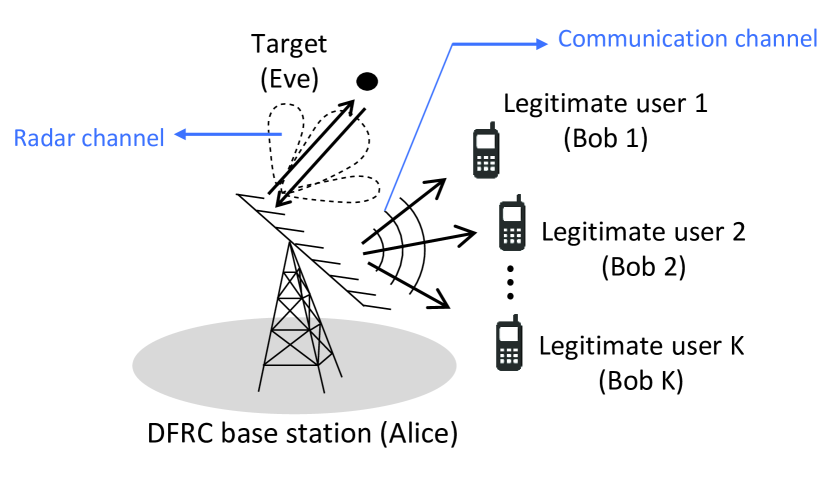
Figure 1: Dual-functional Radar-Communication system detecting target which comprise a potential eavesdropper.

II System Model

We consider a dual-functional MIMO DFRC system, which consists of a DFRC base station, legitimate users and target which is a potential eavesdropper, as shown in Fig. 1. The DFRC system is equipped with uniform linear array (ULA) of N antennas, serving K single-antenna users, while detecting a single point-like target. For convenience, the multi-antenna transmitter, the legitimate users and the target will be referred as Alice, Bobs and Eve respectively.

II-A Signal Model

In the scenario shown in Fig. 1, the DFRC base station Alice intends to send confidential information to single-antenna legitimate users, i.e. Bobs, with the presence of the potential eavesdropper, i.e. Eve. The received symbol vector at Bobs can be modeled as

$${\mathbf{y}={\mathbf{H}}\mathbf{x}+\mathbf{z}}\,$$ (1)

where ${\mathbf{H}}={\left[{{{\mathbf{h}}_{1}},{{\mathbf{h}}_{2}},\cdots,{{\mathbf{h}}_{K}}}\right]^{T}}\in{\mathbb{C}^{K\times N}}$ is the channel matrix, ${\mathbf{x}}\in{\mathbb{C}^{N}}$ is the transmitted signal vector, ${\mathbf{z}}$ is the noise vector, with ${{\mathbf{z}}}\sim\mathcal{C}\mathcal{N}\left({0,{\sigma^{2}}{\mathbf{I}}_{N}}\right)$.
Consider AN-aided transmit beamforming, the transmit vector ${\mathbf{x}}$ can be written as

$${\mathbf{x}=\mathbf{W}\mathbf{s}+\mathbf{n}}\,$$ (2)

where ${\mathbf{s}}\in{\mathbb{C}^{K}}$ is the desired symbol vector of Bobs, where we assume $\mathbb{E}\left[{{\mathbf{s}}}\mathbf{s}^{H}\right]={\mathbf{I}}$, ${\mathbf{W}}=\left[{{{\mathbf{w}}_{1}},{{\mathbf{w}}_{2}},\cdots,{{\mathbf{w}}_{K}}}\right]\in{\mathbb{C}^{N\times K}}$ is the beamforming matrix, ${\mathbf{n}}$ is an artificial noise vector generated by Alice to avoid leaking information to Eves. It is assumed that ${{\mathbf{n}}}\sim\mathcal{C}\mathcal{N}\left({0,{{\mathbf{R}}_{N}}}\right)$. Additionally, we assume that the desired symbol vector $\mathbf{s}$ and the artificial noise vector $\mathbf{n}$ are independent with each other.
According to [9], it is presumed that the above signal is used for both radar and communication operations, where each communication symbol is considered as a snapshot of a radar pulse. Then, the covariance matrix of radar system can be given as

$${{\mathbf{R}}_{X}}=\mathbb{E}\left[{\mathbf{x}}{{\mathbf{x}}^{H}}\right]=\sum\limits_{i=1}^{K}{{{\mathbf{W}}_{i}}+{{\mathbf{R}}_{N}}},$$ (3)

where ${{\mathbf{W}}_{i}}\triangleq{{\mathbf{w}}_{i}}\mathbf{w}_{i}^{H}$. Then, the beampattern can be expressed as

$${{P}_{bp}}={{\mathbf{a}}^{H}}\left(\theta\right){{\mathbf{R}}_{X}}\mathbf{a}\left(\theta\right),$$ (4)

where $\theta$ is the angle of target, $\mathbf{a}\left(\theta\right)={{\left[\begin{matrix}1&{{e}^{j2\pi\Delta\sin\left(\theta\right)}}&\cdots&{{e}^{j2\pi\left(N-1\right)\Delta\sin\left(\theta\right)}}\\ \end{matrix}\right]}^{T}}\in{{\mathbb{C}}^{N\times 1}}$ denotes the steering vector of the transmit antenna array, and $\Delta$ is the interval between adjacent antennas being normalized by the wavelength.

II-B Metrics

To evaluate the performance of the system, we define a number of performance metrics in this subsection. Initially, based on the aforementioned system model, the SINR of the i-th user can be written as

$${{\text{SINR}}_{i}} =\frac{\mathbb{E}\left[{{\left|\mathbf{h}_{i}^{T}{{\mathbf{w}}_{i}}{{\mathbf{s}}}\right|}^{2}}\right]}{\sum\nolimits_{k\neq i,k=1}^{K}{\mathbb{E}\left[{{\left|\mathbf{h}_{i}^{T}{{\mathbf{w}}_{k}}{{\mathbf{s}}}\right|}^{2}}\right]+\mathbb{E}\left[{{\left|\mathbf{h}_{i}^{T}{{\mathbf{n}}}\right|}^{2}}\right]+\sigma^{2}}}$$ (5)

$$=\frac{{{\mathbf{h}}_{i}^{T}{{\mathbf{W}}_{i}}{\mathbf{h}}_{i}^{*}}}{{\sum\nolimits_{k\neq i,k=1}^{K}{\left({{\mathbf{h}}_{i}^{T}{{\mathbf{W}}_{k}}{\mathbf{h}}_{i}^{*}}\right)}+\left({{\mathbf{h}}_{i}^{T}{{\mathbf{R}}_{N}}{\mathbf{h}}_{i}^{*}}\right)+{\sigma^{2}}}},$$

where ${{\mathbf{n}}_{i}}$ is the AN of i-th user.
Equation (5) can be simplified

$${{\text{SINR}}_{i}}=\frac{\text{tr}\left(\mathbf{h}_{i}^{*}\mathbf{h}_{i}^{T}{{\mathbf{W}}_{i}}\right)}{\sum\nolimits_{k\neq i,k=1}^{K}{\text{tr}\left(\mathbf{h}_{i}^{*}\mathbf{h}_{i}^{T}{{\mathbf{W}}_{k}}\right)}+\text{tr}\left(\mathbf{h}_{i}^{*}\mathbf{h}_{i}^{T}{{\mathbf{R}}_{N}}\right)+\sigma^{2}}.$$ (6)

The achievable transmission rate of legitimate users is given as

$${R_{{C_{i}}}}={\log_{2}}\left({1+{\text{SIN}}{{\text{R}}_{i}}}\right).$$ (7)

Likewise, based on the given signal model in (3) and (4), SINR at Eve can be given as [35]

$$\text{SIN}{{\text{R}}_{E}}=\frac{{{\left|\alpha\right|}^{2}}{{\mathbf{a}}^{H}}\left(\theta\right)\sum\nolimits_{i=1}^{K}{{{\mathbf{W}}_{i}}}\mathbf{a}\left(\theta\right)}{{{\left|\alpha\right|}^{2}}{{\mathbf{a}}^{H}}\left(\theta\right){{\mathbf{R}}_{N}}\mathbf{a}\left(\theta\right)+\sigma^{2}},$$ (8)

where $\alpha$ represents the propagation loss in radar system. The achievable transmission rate of Eve can be expressed as

$${R_{E}}={\log_{2}}\left({1+{\text{SIN}}{{\text{R}}_{E}}}\right).$$ (9)

Additionally, the transmit power is expressed as

$${{P}_{t}}=\text{tr}({{\mathbf{R}}_{X}}).$$ (10)

Given the achievable transmission rates of Bobs and Eve, the achievable secrecy rate of the system is defined as [36]

$${\text{SR}}=\mathop{\min}\limits_{i}\frac{1}{2}{\left[{{R_{{C_{i}}}}-{R_{E}}}\right]^{+}}.$$ (11)

III Minimizing SINR of Eve With Premise of Perfect CSI and Target Direction

In this section, we aim to enhance the secrecy rate by minimizing the SINR of Eve and setting a lower threshold of SINR for the legitimate users, i.e. Bobs. The optimization problem is based on the assumption that the channel information from Alice to Bobs in the communication system is known perfectly. Meanwhile, the precise direction of the detected target is known to the transmitter. We shall relax the above assumptions in the following sections.

III-A Problem Formulation

Let us firstly consider the $\text{SINR}_{E}$ minimization problem, which should guarantee: a) individual SINR requirement at each legitimate user, b) transmit power budget and c) a desired radar spatial beampattern. Note that an ideal radar beampattern should be obtained before designing the beamforming and artificial noise, which can be generated by solving the following constrained least-squares (LS) problem [9, 37] as an example

$$\begin{gathered}\mathop{\min}\limits_{\eta,{{\mathbf{R}}_{d}}}\;{\sum\limits_{m=1}^{M}{\left|{\eta{P_{d}}\left({{\theta_{m}}}\right)-{{\mathbf{a}}^{H}}\left({{\theta_{m}}}\right){{\mathbf{R}}_{d}}{\mathbf{a}}\left({{\theta_{m}}}\right)}\right|}^{2}}\hfill\\ s.t.\;\;\;{\text{tr}}\left({{{\mathbf{R}}_{d}}}\right)={P_{0}},\hfill\\ \;\;\;\;\;\;\;\;{{\mathbf{R}}_{d}}\succeq 0,{{\mathbf{R}}_{d}}={\mathbf{R}}_{d}^{H},\hfill\\ \;\;\;\;\;\;\;\;\eta\geq 0,\hfill\\ \end{gathered}$$ (12)

where $\eta$ is a scaling factor, ${P_{0}}$ represents the transmission power budget, $\left\{{{\theta_{m}}}\right\}_{m=1}^{M}$ denotes an angular grid covering the detection angular range in $\left[{{-}\pi/2,\pi/2}\right]$, ${{\mathbf{a}}\left({{\theta_{m}}}\right)}$ denotes steering vector, ${{P_{d}}\left({{\theta_{m}}}\right)}$ is the desired ideal beampattern gain at ${\theta_{m}}$, ${{{\mathbf{R}}_{d}}}$ represents the desired waveform covariance matrix.
Given a covariance matrix ${{{\mathbf{R}}_{d}}}$ that corresponds to a well-designed MIMO radar beampattern, the fractional programming optimization problem of minimizing ${{\text{SIN}}{{\text{R}}_{E}}}$ can be formulated as

$$\mathop{\min}\limits_{{{\mathbf{W}}_{i}},{{\mathbf{R}}_{N}}}\frac{{{\left|\alpha\right|}^{2}}{{\mathbf{a}}^{H}}\left(\theta_{0}\right)\sum\nolimits_{i=1}^{K}{{{\mathbf{W}}_{i}}}\mathbf{a}\left(\theta_{0}\right)}{{{\left|\alpha\right|}^{2}}{{\mathbf{a}}^{H}}\left(\theta_{0}\right){{\mathbf{R}}_{N}}\mathbf{a}\left(\theta_{0}\right)+\sigma^{2}},\hfill$$ (13a)

$$s.t.\;\;\;{\left\|{{{\mathbf{R}}_{X}}-{{\mathbf{R}}_{d}}}\right\|^{2}}\leq{\gamma_{bp}},\hfill$$ (13b)

$$\;\;\;\;\;\;\;\;{\text{SIN}}{{\text{R}}_{i}}\geq{\gamma_{b}},\forall i,\hfill$$ (13c)

$$\;\;\;\;\;\;\;\;\text{tr}({{\mathbf{R}}_{X}})={P_{0}},\hfill$$ (13d)

$$\;\;\;\;\;\;\;\;{{\mathbf{W}}_{i}}={\mathbf{W}}_{i}^{H},{{\mathbf{W}}_{i}}\succeq 0,\forall i,\hfill$$ (13e)

$$\;\;\;\;\;\;\;\;{\text{rank}}\left({{{\mathbf{W}}_{i}}}\right)=1,\forall i,\hfill$$ (13f)

$$\;\;\;\;\;\;\;\;{{\mathbf{R}}_{N}}={\mathbf{R}}_{N}^{H},{{\mathbf{R}}_{N}}\succeq 0,$$ (13g)

where the constraints ${{\mathbf{W}}_{i}}={\mathbf{W}}_{i}^{H},{{\mathbf{W}}_{i}}\succeq 0,{\text{rank}}\left({{{\mathbf{W}}_{i}}}\right)=1,\forall i,$ are equivalent to constraining ${{\mathbf{W}}_{i}}={{\mathbf{w}}_{i}}\mathbf{w}_{i}^{H}$ [20]. $\theta_{0}$ represents the direction of Eve known at Alice, ${\gamma_{bp}}$ is the pre-defined threshold that constraints the mismatch between designed covariance matrix ${{{\mathbf{R}}_{X}}}$ and the desired ${{{\mathbf{R}}_{d}}}$, and finally ${\gamma_{b}}$ denotes the predefined SINR threshold of each legitimate user.
First, let us employ the SDR approach by relaxing the optimization problem by omitting the ${\text{rank}}\left({{{\mathbf{W}}_{i}}}\right)=1$ constraint in (13f), which can be written as

$$\mathop{\min}\limits_{{{\mathbf{W}}_{i}},{{\mathbf{R}}_{N}}}\frac{{{\left|\alpha\right|}^{2}}{{\mathbf{a}}^{H}}\left(\theta_{0}\right)\sum\nolimits_{i=1}^{K}{{{\mathbf{W}}_{i}}}\mathbf{a}\left(\theta_{0}\right)}{{{\left|\alpha\right|}^{2}}{{\mathbf{a}}^{H}}\left(\theta_{0}\right){{\mathbf{R}}_{N}}\mathbf{a}\left(\theta_{0}\right)+\sigma^{2}},\hfill$$ (14a)

$$s.t.\;\;\;{\left\|{{{\mathbf{R}}_{X}}-{{\mathbf{R}}_{d}}}\right\|^{2}}\leq{\gamma_{bp}},\hfill$$ (14b)

$$\;\;\;\;\;\;\;\;{\text{SIN}}{{\text{R}}_{i}}\geq{\gamma_{b}},\forall i,\hfill$$ (14c)

$$\;\;\;\;\;\;\;\;\text{tr}({{\mathbf{R}}_{X}})={P_{0}},\hfill$$ (14d)

$$\;\;\;\;\;\;\;\;{{\mathbf{W}}_{i}}={\mathbf{W}}_{i}^{H},{{\mathbf{W}}_{i}}\succeq 0,\forall i,\hfill$$ (14e)

$$\;\;\;\;\;\;\;\;{{\mathbf{R}}_{N}}={\mathbf{R}}_{N}^{H},{{\mathbf{R}}_{N}}\succeq 0.$$ (14f)

By noting the fact that problem (14) is still non-convex due to the fractional objective function, we propose in the following an iterative approach to solve the problem efficiently.

III-B Efficient Solver

Following [33], (14) is single-ratio FP problem, which can be solved by employing the Dinkelbach’s transform demonstrated in [38], where the globally optimal solution can be obtained by solving a sequence of SDPs. To develop the algorithm, we firstly introduce a scaling factor $c={\text{SIN}}{{\text{R}}_{E}}$, which is an auxiliary variable. We then define two scaling variables $\operatorname{U}$ and $\operatorname{V}$, which are nonnegative and positive respectively, where $\operatorname{U}={\left|\alpha\right|^{2}}{{\mathbf{a}}^{H}}\left(\theta\right)\sum\nolimits_{i=1}^{K}{{{\mathbf{W}}_{i}}}{\mathbf{a}}\left(\theta\right),\forall i$, $\operatorname{V}={\left|\alpha\right|^{2}}{{\mathbf{a}}^{H}}\left(\theta\right){{\mathbf{R}}_{N}}{\mathbf{a}}\left(\theta\right)+{\sigma^{2}}$. As a result, the FP problem (14) can be reformulated as

$$\mathop{\min}\limits_{{{\mathbf{W}}_{i}},{{\mathbf{R}}_{N}}}\operatorname{U}-c\operatorname{V},\hfill$$ (15a)

$$s.t.\;\;\;{\left\|{{{\mathbf{R}}_{X}}-{{\mathbf{R}}_{d}}}\right\|^{2}}\leq{\gamma_{bp}},\hfill$$ (15b)

$$\;\;\;\;\;\;\;\;{\text{SIN}}{{\text{R}}_{i}}\geq{\gamma_{b}},\forall i,\hfill$$ (15c)

$$\;\;\;\;\;\;\;\;\text{tr}({{\mathbf{R}}_{X}})={P_{0}},\hfill$$ (15d)

$$\;\;\;\;\;\;\;\;{{\mathbf{W}}_{i}}={\mathbf{W}}_{i}^{H},{{\mathbf{W}}_{i}}\succeq 0,\forall i,\hfill$$ (15e)

$$\;\;\;\;\;\;\;\;{{\mathbf{R}}_{N}}={\mathbf{R}}_{N}^{H},{{\mathbf{R}}_{N}}\succeq 0,$$ (15f)

where $c$ can be iteratively updated by

$$c\left[{t+1}\right]=\frac{{\operatorname{U}\left[t\right]}}{{\operatorname{V}\left[t\right]}},$$ (16)

where $t$ is the index of iteration. For clarity, we summarize the above in Algorithm 1. According to [33], it is easy to prove the convergence of the algorithm given the non-increasing property of $c$ during each iteration. It is noted that the SDR approach generates an approximated solution to the optimization problem (13) by neglecting the rank-one constraint. Accordingly, eigenvalue decomposition or Gaussian randomization techniques are commonly employed to obtain a suboptimal solution.

Algorithm 1 Alogrithm for solving FP problem (14)

0:  ${\mathbf{H}},{\mathbf{a}}\left(\theta_{0}\right),{\sigma^{2}},\alpha,{\gamma_{bp}},{\gamma_{b}},{P_{0}},ite{r_{max}}\geq 2$

0:  ${\mathbf{W}}_{i}^{\left({iter}\right)},{\mathbf{R}}_{N}^{\left({iter}\right)},i=1,\cdots,K$

  1. Compute ${{\mathbf{R}}_{d}}$. Reformulate problem (13a) by (14). Set the iteration threshold $\varepsilon>0$. Initialize ${c^{\left(0\right)}},{c^{\left(1\right)}},\left|{{c^{\left(1\right)}}-{c^{\left(0\right)}}}\right|>\varepsilon$.

  while $iter\leq ite{r_{max}}$ and $\left|{{c^{iter+1}}-{c^{iter}}}\right|\geq\varepsilon$  do

     2. Solve the SDP problem (15).

     3. Update $c$ by (16).

     4. $iter=iter+1$.

  end while

  6. Obtain approximated solutions by eigenvalue decomposition or Gaussian randomization.

III-C Complexity Analysis

In this subsection, the computational complexity of Algorithm 1 is analyzed as follows. Note that SDP problems are commonly solved by the interior point method (IPM) [39], which obtains an $\epsilon$-optimal solution after a sequence of iterations with the given $\epsilon$. In problem (15), it is noted that the constraints are linear matrix inequality (LMI) except for (15b), which is a second-order cone (SOC) [40] constraint. Besides, we note that the solution is required to satisfy the rank-one constraint, the complexity of eigenvalue decomposition is then taken into consideration, which is operated at the cost of $\mathcal{O}\left({\left({K+1}\right){N^{3}}}\right)$ complex multiplications. Thus, we demonstrate the complexity in Table I, where ${N_{iter}}$ represents iteration times. For simplicity, the computational complexity can be given as $\mathcal{O}\left({\sqrt{2}{N_{iter}}\ln\left({{1\mathord{\left/{\vphantom{1\epsilon}}\right.\kern-1.2pt}\epsilon}}\right){K^{3.5}}{N^{6.5}}}\right)+\mathcal{O}\left({\left({K+1}\right){N^{3}}}\right)$by reserving the highest order term.

IV Eve’s SINR Minimization With Uncertainty in the Target Direction and Perfect CSI

In practice, the precise location of the target is difficult to be known at transmitter. In this section, we consider the scenario where a rough estimate of the target angle, instead of its precise counterpart, is available at Alice. Therefore, the following beampattern design aims at achieving both a desired main-beam width covering the possible angle uncertainty interval of the target as well as a minimized sidelobe power in a prescribed region.

IV-A Problem Formulation

In this subsection, we consider the case that the angle uncertainty interval of the target is roughly known within the angular interval $\left[{{\theta_{0}}-\Delta\theta,{\theta_{0}}+\Delta\theta}\right]$. To this end, the target from every possible direction should be taken in to consideration when formulating the optimization problem. Accordingly, the objective is given as the sum of Eve’s SINR at all the possible locations as follows. Due to the uncertainty of target location, wider beampattern needs to be formulated towards the uncertain angular interval to avoid missing the target. Inspired by the 3dB main-beam width beampattern design for MIMO radar [41], we propose a scheme aiming at keeping a constant power in the uncertain angular interval, which can be formulated as the following optimization problem

$$\mathop{\min}\limits_{{{\mathbf{W}}_{i}},{{\mathbf{R}}_{X}}}\sum\limits_{{\theta_{m}}\in\Phi}{\frac{{{{\left|\alpha\right|}^{2}}{{\mathbf{a}}^{H}}\left({{\theta_{m}}}\right)\sum\nolimits_{i=1}^{K}{{{\mathbf{W}}_{i}}}{\mathbf{a}}\left({{\theta_{m}}}\right)}}{{{{\left|\alpha\right|}^{2}}{{\mathbf{a}}^{H}}\left({{\theta_{m}}}\right){{\mathbf{R}}_{N}}{\mathbf{a}}\left({{\theta_{m}}}\right)+{\sigma^{2}}}}}\hfill$$ (17a)

$$s.t.\;\;{{\mathbf{a}}^{H}}\left({{\theta_{0}}}\right){{\mathbf{R}}_{X}}{\mathbf{a}}\left({{\theta_{0}}}\right)-{{\mathbf{a}}^{H}}\left({{\theta_{m}}}\right){{\mathbf{R}}_{X}}{\mathbf{a}}\left({{\theta_{m}}}\right)\geq{\gamma_{s}},$$

$$\;\;\;\;\;\;\;\;\;\;\;\;\;\;\;\;\;\;\;\;\;\;\;\;\;\;\;\;\;\;\;\;\;\;\;\;\;\;\;\;\;\;\;\;\;\;\;\;\;\;\;\;\;\;\;\;\;\;\;\;\;\;\;\;\;\forall{\theta_{m}}\in\Omega\hfill$$ (17b)

$$\;\;\;\;\;\;\;{{\mathbf{a}}^{H}}\left({{\theta_{k}}}\right){{\mathbf{R}}_{X}}{\mathbf{a}}\left({{\theta_{k}}}\right)\leq\left({1+\alpha}\right){{\mathbf{a}}^{H}}\left({{\theta_{0}}}\right){{\mathbf{R}}_{X}}{\mathbf{a}}\left({{\theta_{0}}}\right),$$

$$\;\;\;\;\;\;\;\;\;\;\;\;\;\;\;\;\;\;\;\;\;\;\;\;\;\;\;\;\;\;\;\;\;\;\;\;\;\;\;\;\;\;\;\;\;\;\;\;\;\;\;\;\;\;\;\;\;\;\;\;\;\;\;\;\;\forall{\theta_{k}}\in\Phi\hfill$$ (17c)

$$\;\;\;\;\;\;\;\left({1-\alpha}\right){{\mathbf{a}}^{H}}\left({{\theta_{0}}}\right){{\mathbf{R}}_{X}}{\mathbf{a}}\left({{\theta_{0}}}\right)\leq{{\mathbf{a}}^{H}}\left({{\theta_{k}}}\right){{\mathbf{R}}_{X}}{\mathbf{a}}\left({{\theta_{k}}}\right),$$

$$\;\;\;\;\;\;\;\;\;\;\;\;\;\;\;\;\;\;\;\;\;\;\;\;\;\;\;\;\;\;\;\;\;\;\;\;\;\;\;\;\;\;\;\;\;\;\;\;\;\;\;\;\;\;\;\;\;\;\;\;\;\;\;\;\;\forall{\theta_{k}}\in\Phi\hfill$$ (17d)

$$\;\;\;\;\;\;\;{\text{SIN}}{{\text{R}}_{i}}\geq{\gamma_{b}},\forall i,\hfill$$ (17e)

$$\;\;\;\;\;\;\;\text{tr}({{\mathbf{R}}_{X}})={P_{0}},\hfill$$ (17f)

$$\;\;\;\;\;\;\;{{\mathbf{W}}_{i}}={\mathbf{W}}_{i}^{H},\;{{\mathbf{W}}_{i}}\succeq 0,\forall i,\hfill$$ (17g)

$$\;\;\;\;\;\;\;{\text{rank}}\left({{{\mathbf{W}}_{i}}}\right)=1,\forall i,\hfill$$ (17h)

$$\;\;\;\;\;\;\;{{\mathbf{R}}_{N}}={\mathbf{R}}_{N}^{H},\;{{\mathbf{R}}_{N}}\succeq 0,$$ (17i)

where ${{\theta_{0}}}$ is the main-beam location, ${\Omega}$ denotes the sidelobe region of interest, ${\Phi}$ denotes the wide main-beam region, ${\gamma_{s}}$ is the bound of the sidelobe power.
Likewise, recall the problem (13), SDR technique is adopted by neglecting rank-1 constraint in (17h). To solve the above sum-of-ratio problem, according to [33], we equivalently recast transform the minimization problem as

$$\mathop{\max}\limits_{{{\mathbf{W}}_{i}},{{\mathbf{R}}_{X}}}\sum\limits_{{\theta_{m}}\in\Phi}{\frac{{{{\left|\alpha\right|}^{2}}{{\mathbf{a}}^{H}}\left({{\theta_{m}}}\right){{\mathbf{R}}_{N}}{\mathbf{a}}\left({{\theta_{m}}}\right)+{\sigma^{2}}}}{{{{\left|\alpha\right|}^{2}}{{\mathbf{a}}^{H}}\left({{\theta_{m}}}\right)\sum\nolimits_{i=1}^{K}{{{\mathbf{W}}_{i}}}{\mathbf{a}}\left({{\theta_{m}}}\right)}}}\hfill$$ (18a)

$$s.t.\;\;{{\mathbf{a}}^{H}}\left({{\theta_{0}}}\right){{\mathbf{R}}_{X}}{\mathbf{a}}\left({{\theta_{0}}}\right)-{{\mathbf{a}}^{H}}\left({{\theta_{m}}}\right){{\mathbf{R}}_{X}}{\mathbf{a}}\left({{\theta_{m}}}\right)\geq{\gamma_{s}},$$

$$\;\;\;\;\;\;\;\;\;\;\;\;\;\;\;\;\;\;\;\;\;\;\;\;\;\;\;\;\;\;\;\;\;\;\;\;\;\;\;\;\;\;\;\;\;\;\;\;\;\;\;\;\;\;\;\;\;\;\;\;\;\;\;\;\;\forall{\theta_{m}}\in\Omega\hfill$$ (18b)

$$\;\;\;\;\;\;\;{{\mathbf{a}}^{H}}\left({{\theta_{k}}}\right){{\mathbf{R}}_{X}}{\mathbf{a}}\left({{\theta_{k}}}\right)\leq\left({1+\alpha}\right){{\mathbf{a}}^{H}}\left({{\theta_{0}}}\right){{\mathbf{R}}_{X}}{\mathbf{a}}\left({{\theta_{0}}}\right),$$

$$\;\;\;\;\;\;\;\;\;\;\;\;\;\;\;\;\;\;\;\;\;\;\;\;\;\;\;\;\;\;\;\;\;\;\;\;\;\;\;\;\;\;\;\;\;\;\;\;\;\;\;\;\;\;\;\;\;\;\;\;\;\;\;\;\;\forall{\theta_{k}}\in\Phi\hfill$$ (18c)

$$\;\;\;\;\;\;\;\left({1-\alpha}\right){{\mathbf{a}}^{H}}\left({{\theta_{0}}}\right){{\mathbf{R}}_{X}}{\mathbf{a}}\left({{\theta_{0}}}\right)\leq{{\mathbf{a}}^{H}}\left({{\theta_{k}}}\right){{\mathbf{R}}_{X}}{\mathbf{a}}\left({{\theta_{k}}}\right),$$

$$\;\;\;\;\;\;\;\;\;\;\;\;\;\;\;\;\;\;\;\;\;\;\;\;\;\;\;\;\;\;\;\;\;\;\;\;\;\;\;\;\;\;\;\;\;\;\;\;\;\;\;\;\;\;\;\;\;\;\;\;\;\;\;\;\;\forall{\theta_{k}}\in\Phi\hfill$$ (18d)

$$\;\;\;\;\;\;\;{\text{SIN}}{{\text{R}}_{i}}\geq{\gamma_{b}},\forall i,\hfill$$ (18e)

$$\;\;\;\;\;\;\;\text{tr}({{\mathbf{R}}_{X}})={P_{0}},\hfill$$ (18f)

$$\;\;\;\;\;\;\;{{\mathbf{W}}_{i}}={\mathbf{W}}_{i}^{H},\;{{\mathbf{W}}_{i}}\succeq 0,\forall i,\hfill$$ (18g)

$$\;\;\;\;\;\;\;{{\mathbf{R}}_{N}}={\mathbf{R}}_{N}^{H},\;{{\mathbf{R}}_{N}}\succeq 0.$$ (18h)

It is noted that problem (18) is still non-convex. The approach to solve this sum-of-ratio FP problem is described in the following.

IV-B Efficient Solver

To present the solution to problem (18), we firstly refer to [33] and denote

$$A\left({{\theta_{m}}}\right)={\left|\alpha\right|^{2}}{{\mathbf{a}}^{H}}\left({{\theta_{m}}}\right){{\mathbf{R}}_{N}}{\mathbf{a}}\left({{\theta_{m}}}\right)+{\sigma^{2}}\hfill$$

$$B\left({{\theta_{m}}}\right)={\left|\alpha\right|^{2}}{{\mathbf{a}}^{H}}\left({{\theta_{m}}}\right)\sum\nolimits_{i=1}^{K}{{{\mathbf{W}}_{i}}}{\mathbf{a}}\left({{\theta_{m}}}\right)$$

One step further, the sum-of-ratio problem is equivalent to the following optimization problem, which can be rewritten in the form

$$\mathop{\max}\limits_{{{\mathbf{W}}_{i}},{{\mathbf{R}}_{N}},{\mathbf{y}}}\sum\limits_{{\theta_{m}}\in\Phi}{\left({2{y_{m}}\sqrt{A\left({{\theta_{m}}}\right)}-y_{m}^{2}B\left({{\theta_{m}}}\right)}\right)},\hfill$$ (19a)

$$s.t.\;\;{{\mathbf{a}}^{H}}\left({{\theta_{0}}}\right){{\mathbf{R}}_{X}}{\mathbf{a}}\left({{\theta_{0}}}\right)-{{\mathbf{a}}^{H}}\left({{\theta_{m}}}\right){{\mathbf{R}}_{X}}{\mathbf{a}}\left({{\theta_{m}}}\right)\geq{\gamma_{s}},$$

$$\;\;\;\;\;\;\;\;\;\;\;\;\;\;\;\;\;\;\;\;\;\;\;\;\;\;\;\;\;\;\;\;\;\;\;\;\;\;\;\;\;\;\;\;\;\;\;\;\;\;\;\;\;\;\;\;\;\;\;\;\;\;\;\;\;\forall{\theta_{m}}\in\Omega\hfill$$ (19b)

$$\;\;\;\;\;\;\;{{\mathbf{a}}^{H}}\left({{\theta_{k}}}\right){{\mathbf{R}}_{X}}{\mathbf{a}}\left({{\theta_{k}}}\right)\leq\left({1+\alpha}\right){{\mathbf{a}}^{H}}\left({{\theta_{0}}}\right){{\mathbf{R}}_{X}}{\mathbf{a}}\left({{\theta_{0}}}\right),$$

$$\;\;\;\;\;\;\;\;\;\;\;\;\;\;\;\;\;\;\;\;\;\;\;\;\;\;\;\;\;\;\;\;\;\;\;\;\;\;\;\;\;\;\;\;\;\;\;\;\;\;\;\;\;\;\;\;\;\;\;\;\;\;\;\;\;\forall{\theta_{k}}\in\Phi\hfill$$ (19c)

$$\;\;\;\;\;\;\;\left({1-\alpha}\right){{\mathbf{a}}^{H}}\left({{\theta_{0}}}\right){{\mathbf{R}}_{X}}{\mathbf{a}}\left({{\theta_{0}}}\right)\leq{{\mathbf{a}}^{H}}\left({{\theta_{k}}}\right){{\mathbf{R}}_{X}}{\mathbf{a}}\left({{\theta_{k}}}\right),$$

$$\;\;\;\;\;\;\;\;\;\;\;\;\;\;\;\;\;\;\;\;\;\;\;\;\;\;\;\;\;\;\;\;\;\;\;\;\;\;\;\;\;\;\;\;\;\;\;\;\;\;\;\;\;\;\;\;\;\;\;\;\;\;\;\;\;\forall{\theta_{k}}\in\Phi\hfill$$ (19d)

$$\;\;\;\;\;\;\;{\text{SIN}}{{\text{R}}_{i}}\geq{\gamma_{b}},\forall i,\hfill$$ (19e)

$$\;\;\;\;\;\;\;\text{tr}({{\mathbf{R}}_{X}})={P_{0}},\hfill$$ (19f)

$$\;\;\;\;\;\;\;{{\mathbf{W}}_{i}}={\mathbf{W}}_{i}^{H},\;{{\mathbf{W}}_{i}}\succeq 0,\forall i,\hfill$$ (19g)

$$\;\;\;\;\;\;\;{{\mathbf{R}}_{N}}={\mathbf{R}}_{N}^{H},\;{{\mathbf{R}}_{N}}\succeq 0,$$ (19h)

where ${\mathbf{y}}$ denotes a collection of variables $\left\{{{y_{1}},\cdots,{y_{M}}}\right\}$. The optimal ${y_{m}}$ can be obtained in the following closed form when $\theta_{m}$ is fixed

$$y_{m}^{*}=\frac{{\sqrt{A\left({{\theta_{m}}}\right)}}}{{B\left({{\theta_{m}}}\right)}}.$$ (20)

To this end, the problem (19) can be solved by the SDR technique. Then, eigenvalue decomposition or Gaussian randomization is required to get the approximated solution. For clarity, the above procedure is summarized in Algorithm 2.

Algorithm 2 Algorithm for solving sum-of-ratio problem (19)

0:  ${\mathbf{H}},{\mathbf{a}}\left(\theta\right)$ or ${\mathbf{a}}\left(\theta_{m}\right)$, ${\sigma^{2}},\alpha,{\gamma_{b}},{P_{0}},ite{r_{max}}\geq 2$, $\Delta\theta$.

0:  ${\mathbf{W}}_{i}^{\left({iter}\right)},{\mathbf{R}}_{N}^{\left({iter}\right)},i=1,\cdots,K$.

  1. Compute ${{\mathbf{R}}_{d}}$. Reformulate problem (17) by (19). Set the iteration threshold $\varepsilon>0$.

  while $iter\leq ite{r_{max}}$ and $\left\|{{{\mathbf{y}}^{iter+1}}-{{\mathbf{y}}^{iter}}}\right\|\geq\varepsilon$ do

     2. Solve the new convex optimization problem.

     3. Update ${\mathbf{y}}$ by (20).

     4. Get updated ${{\mathbf{W}}_{i}},\forall i,$ and ${{\mathbf{R}}_{N}}$ by solving (19) using SDR.

     5. $iter=iter+1$.

  end while

  6. Obtain approximate solutions by eigenvalue decomposition or Gaussian randomization.

IV-C Complexity Analysis

We end this section by computing the complexity of solving problem (19). It is noted that all the constraints can be considered as LMIs in optimization problem (19). We denote $\Phi_{0}=card(\Phi)$ and $\Omega_{0}=card(\Omega)$ as the cardinality of $\Phi$ and $\Omega$, respectively. Likely, eigenvalue decomposition operation is required as well, with the cost of $O\left({\left({K+1}\right){N^{3}}}\right)$. Thus, referring to [39], we give the computational complexity in Table I, which can be simplified as $\mathcal{O}\left({3\sqrt{2}{N_{iter}}\ln\left({{1\mathord{\left/{\vphantom{1\epsilon}}\right.\kern-1.2pt}\epsilon}}\right){K^{3.5}}{N^{6.5}}}\right)+\mathcal{O}\left({\left({K+1}\right){N^{3}}}\right)$ by reserving the highest order.

V Robust Beamforming With Imperfect CSI And Target Direction Uncertainty

In this section, based on the models presented in the previous sections, we consider the case that perfect channel information is not available at the base station. By relying on the method of robust optimization, we generalize an optimization problem to obtain beamforming design that is robust to the channel uncertainty, which is bounded in a spherical region. Meanwhile, to guarantee the generality, we minimize the worst-case SINR received at the target in the angular interval of possible location of potential eavesdropper.

V-A Problem Formulation

According to [42], an additive channel error model of $i$-th downlink user can be formulated as ${{\mathbf{h}}_{i}}={{\mathbf{\tilde{h}}}_{i}}+{{\mathbf{e}}_{i}}$, where ${{\mathbf{\tilde{h}}}_{i}}$ is the estimated channel information known at Alice, and ${{\mathbf{e}}_{i}}$ denotes the channel uncertainty within the spherical region ${\Im_{i}}=\{{{\mathbf{e}}_{i}}|{\left\|{{{\mathbf{e}}_{i}}}\right\|^{2}}\leq{\mathbf{\mu}}_{i}^{2}\}$. Following the well-known S-procedure , $\forall{\mathbf{e}}_{i}^{H}{{\mathbf{e}}_{i}}\leq\mu_{i}^{2}$ , the constraint that guarantees the worst-case SINR of legitimates users can be reformulated as

$$\begin{split}&{\left({{{{\mathbf{\tilde{h}}}}_{i}}+{{\mathbf{e}}_{i}}}\right)^{H}}\left({{{\mathbf{W}}_{i}}-{\gamma_{b}}\sum\limits_{k=1,k\neq i}^{K}{{{\mathbf{W}}_{k}}}-{\gamma_{b}}{{\mathbf{R}}_{N}}}\right)\left({{{{\mathbf{\tilde{h}}}}_{i}}+{{\mathbf{e}}_{i}}}\right)\hfill\\ &-{\gamma_{b}}{\sigma^{2}}\geq 0,\forall i.\end{split}$$ (21)

Then, we minimize the possible maximum Eve SINR in the main-beam region of interest, which yields the following robust optimization problem

$$\mathop{\min}\limits_{{{\mathbf{W}}_{i}},{{\mathbf{R}}_{N}},{t_{i}}}\mathop{\max}\limits_{{\theta_{m}}\in\Phi}\frac{{{{\left|\alpha\right|}^{2}}{{\mathbf{a}}^{H}}\left({{\theta_{m}}}\right)\sum\nolimits_{i=1}^{K}{{{\mathbf{W}}_{i}}}{\mathbf{a}}\left({{\theta_{m}}}\right)}}{{{{\left|\alpha\right|}^{2}}{{\mathbf{a}}^{H}}\left({{\theta_{m}}}\right){{\mathbf{R}}_{N}}{\mathbf{a}}\left({{\theta_{m}}}\right)+{\sigma^{2}}}}\hfill$$ (22a)

$$s.t.\left({\begin{array}[]{*{20}{c}}{{\mathbf{\tilde{h}}}_{i}^{T}{{\mathbf{Y}}_{i}}{\mathbf{\tilde{h}}}_{i}^{*}-{\gamma_{b}}{\sigma^{2}}-{t_{i}}\mu_{i}^{2}}&{{\mathbf{\tilde{h}}}_{i}^{T}{{\mathbf{Y}}_{i}}}\\ {{{\mathbf{Y}}_{i}}{\mathbf{\tilde{h}}}_{i}^{*}}&{{{\mathbf{Y}}_{i}}+{t_{i}}{{\mathbf{I}}_{N}}}\end{array}}\right)\succeq 0,\forall i,\hfill$$ (22d)

$$\;\;\;\;{{\mathbf{Y}}_{i}}:={{\mathbf{W}}_{i}}-{\gamma_{b}}\left({\sum\limits_{k\neq i}{{{\mathbf{W}}_{k}}}}\right)-{\gamma_{b}}{{\mathbf{R}}_{N}}\hfill$$

$$\;\;\;\;{{\mathbf{a}}^{H}}\left({{\theta_{0}}}\right){{\mathbf{R}}_{X}}{\mathbf{a}}\left({{\theta_{0}}}\right)-{{\mathbf{a}}^{H}}\left({{\theta_{m}}}\right){{\mathbf{R}}_{X}}{\mathbf{a}}\left({{\theta_{m}}}\right)\geqslant{\gamma_{s}},$$

$$\;\;\;\;\;\;\;\;\;\;\;\;\;\;\;\;\;\;\;\;\;\;\;\;\;\;\;\;\;\;\;\;\;\;\;\;\;\;\;\;\;\;\;\;\;\;\;\;\;\;\;\;\;\;\;\;\;\;\;\;\;\;\;\;\;\forall{\theta_{m}}\in\Omega\hfill$$ (22e)

$$\;\;\;\;{{\mathbf{a}}^{H}}\left({{\theta_{k}}}\right){{\mathbf{R}}_{X}}{\mathbf{a}}\left({{\theta_{k}}}\right)\leqslant\left({1+\alpha}\right){{\mathbf{a}}^{H}}\left({{\theta_{0}}}\right){{\mathbf{R}}_{X}}{\mathbf{a}}\left({{\theta_{0}}}\right),\hfill$$

$$\;\;\;\;\;\;\;\;\;\;\;\;\;\;\;\;\;\;\;\;\;\;\;\;\;\;\;\;\;\;\;\;\;\;\;\;\;\;\;\;\;\;\;\;\;\;\;\;\;\;\;\;\;\;\;\;\;\;\;\;\;\;\;\;\;\forall{\theta_{k}}\in\Phi\hfill$$ (22f)

$$\;\;\;\;\left({1-\alpha}\right){{\mathbf{a}}^{H}}\left({{\theta_{0}}}\right){{\mathbf{R}}_{X}}{\mathbf{a}}\left({{\theta_{0}}}\right)\leqslant{{\mathbf{a}}^{H}}\left({{\theta_{k}}}\right){{\mathbf{R}}_{X}}{\mathbf{a}}\left({{\theta_{k}}}\right),\hfill$$

$$\;\;\;\;\;\;\;\;\;\;\;\;\;\;\;\;\;\;\;\;\;\;\;\;\;\;\;\;\;\;\;\;\;\;\;\;\;\;\;\;\;\;\;\;\;\;\;\;\;\;\;\;\;\;\;\;\;\;\;\;\;\;\;\;\;\forall{\theta_{k}}\in\Phi\hfill$$ (22g)

$$\;\;\;\;\text{tr}({{\mathbf{R}}_{X}})={P_{0}},\hfill$$ (22h)

$$\;\;\;\;{t_{i}}\geqslant 0,\forall i,\hfill$$ (22i)

$$\;\;\;\;{{\mathbf{W}}_{i}}={\mathbf{W}}_{i}^{H},{{\mathbf{W}}_{i}}\succeq 0,\forall i,\hfill$$ (22j)

$$\;\;\;\;{\text{rank}}\left({{{\mathbf{W}}_{i}}}\right)=1,\forall i,\hfill$$ (22k)

$$\;\;\;\;{{\mathbf{R}}_{N}}={\mathbf{R}}_{N}^{H},{{\mathbf{R}}_{N}}\succeq 0,$$ (22l)

where $\Phi=\left[{{\theta_{0}}-\Delta\theta,{\theta_{0}}+\Delta\theta}\right]$ is the main-beam region of interest, $m=1,\cdots,M$. $M$ represents the number of detecting angles in the interval $\Phi$, and finally ${\mathbf{t}}=\left[{{t_{1}},\cdots,{t_{K}}}\right]$ is an auxiliary vector relying on the S-procedure.

V-B Efficient Solver

To solve problem (22), the SDR approach is adopted again by dropping the rank-1 constraint in (22i). Moreover, the objective function (22a) can be transformed to a max-min problem initially which is given as

$$\mathop{\max}\limits_{{{\mathbf{W}}_{i}},{{\mathbf{R}}_{N}},{t_{i}}}\mathop{\min}\limits_{{\theta_{m}}\in\Phi}\frac{{{{\left|\alpha\right|}^{2}}{{\mathbf{a}}^{H}}\left({{\theta_{m}}}\right){{\mathbf{R}}_{N}}{\mathbf{a}}\left({{\theta_{m}}}\right)+{\sigma^{2}}}}{{{{\left|\alpha\right|}^{2}}{{\mathbf{a}}^{H}}\left({{\theta_{m}}}\right)\sum\nolimits_{i=1}^{K}{{{\mathbf{W}}_{i}}}{\mathbf{a}}\left({{\theta_{m}}}\right)}}.$$ (23)

To verify this, we introduce a variable $z$ and define ${\mathbf{A}}\left({{\theta_{m}}}\right)={\mathbf{a}}\left({{\theta_{m}}}\right){{\mathbf{a}}^{H}}\left({{\theta_{m}}}\right)$. The objective function (23) can be rewritten as $\mathop{\max}\limits_{{{\mathbf{W}}_{i}},{{\mathbf{R}}_{N}},{t_{i}},z}z$ , which subjects to $z\leq{{\left({{\text{tr}}\left({{\mathbf{A}}\left({{\theta_{m}}}\right){{\mathbf{R}}_{N}}}\right)+{{{\sigma^{2}}}\mathord{\left/{\vphantom{{{\sigma^{2}}}{{{\left|\alpha\right|}^{2}}}}}\right.\kern-1.2pt}{{{\left|\alpha\right|}^{2}}}}}\right)}\mathord{\left/{\vphantom{{\left({{\text{tr}}\left({{\mathbf{A}}\left({{\theta_{m}}}\right){{\mathbf{R}}_{N}}}\right)+{{{\sigma^{2}}}\mathord{\left/{\vphantom{{{\sigma^{2}}}{{{\left|\alpha\right|}^{2}}}}}\right.\kern-1.2pt}{{{\left|\alpha\right|}^{2}}}}}\right)}{{\text{tr}}\left({{\mathbf{A}}\left({{\theta_{m}}}\right)\sum\nolimits_{i=1}^{K}{{{\mathbf{W}}_{i}}}}\right)}}}\right.\kern-1.2pt}{{\text{tr}}\left({{\mathbf{A}}\left({{\theta_{m}}}\right)\sum\nolimits_{i=1}^{K}{{{\mathbf{W}}_{i}}}}\right)}}$ and any other contraints in (19). Likewise, we denote

$$C\left({{\theta_{m}}}\right)={{{\text{tr}}\left({{\mathbf{A}}\left({{\theta_{m}}}\right){{\mathbf{R}}_{N}}}\right)+{{{\sigma^{2}}}\mathord{\left/{\vphantom{{{\sigma^{2}}}{{{\left|\alpha\right|}^{2}}}}}\right.\kern-1.2pt}{{{\left|\alpha\right|}^{2}}}}}}\hfill$$

$$D\left({{\theta_{m}}}\right)=\mathord{{\vphantom{{\left({{\text{tr}}\left({{\mathbf{A}}\left({{\theta_{m}}}\right){{\mathbf{R}}_{N}}}\right)+{{{\sigma^{2}}}\mathord{\left/{\vphantom{{{\sigma^{2}}}{{{\left|\alpha\right|}^{2}}}}}\right.\kern-1.2pt}{{{\left|\alpha\right|}^{2}}}}}\right)}{{\text{tr}}\left({{\mathbf{A}}\left({{\theta_{m}}}\right)\sum\nolimits_{i=1}^{K}{{{\mathbf{W}}_{i}}}}\right)}}}\kern-1.2pt}{{\text{tr}}\left({{\mathbf{A}}\left({{\theta_{m}}}\right)\sum\nolimits_{i=1}^{K}{{{\mathbf{W}}_{i}}}}\right)}$$

The aforementioned constraint is equivalent to

$$z\leq{\max_{{y_{m}}}}\left({2{y_{m}}\sqrt{C\left({{\theta_{m}}}\right)}-y_{m}^{2}D\left({{\theta_{m}}}\right)}\right),$$

which is a less-than-max inequality, so $\mathop{\max}\limits_{{y_{m}}}$ can be integrated into the objective. Consequently, problem (22) is reformulated as

$$\mathop{\max}\limits_{{{\mathbf{W}}_{i}},{{\mathbf{R}}_{N}},{\mathbf{y}},{t_{i}},z}z,$$ (24a)

$$\begin{split}&s.t.\;\;\;2{y_{m}}\sqrt{C\left({{\theta_{m}}}\right)}-y_{m}^{2}{D\left({{\theta_{m}}}\right)}\geq z,{\theta_{m}}\in\Phi,\forall m,\\ \end{split}$$ (24b)

$$\;\;\;\;\left({\begin{array}[]{*{20}{c}}{{\mathbf{\tilde{h}}}_{i}^{T}{{\mathbf{Y}}_{i}}{\mathbf{\tilde{h}}}_{i}^{*}-{\gamma_{b}}{\sigma^{2}}-{t_{i}}\mu_{i}^{2}}&{{\mathbf{\tilde{h}}}_{i}^{T}{{\mathbf{Y}}_{i}}}\\ {{{\mathbf{Y}}_{i}}{\mathbf{\tilde{h}}}_{i}^{*}}&{{{\mathbf{Y}}_{i}}+{t_{i}}{{\mathbf{I}}_{N}}}\end{array}}\right)\succeq 0,\forall i,\hfill$$ (24e)

$$\;\;\;\;{{\mathbf{Y}}_{i}}:={{\mathbf{W}}_{i}}-{\gamma_{b}}\left({\sum\limits_{k\neq i}{{{\mathbf{W}}_{k}}}}\right)-{\gamma_{b}}{{\mathbf{R}}_{N}}\hfill$$

$$\;\;\;\;{{\mathbf{a}}^{H}}\left({{\theta_{0}}}\right){{\mathbf{R}}_{X}}{\mathbf{a}}\left({{\theta_{0}}}\right)-{{\mathbf{a}}^{H}}\left({{\theta_{m}}}\right){{\mathbf{R}}_{X}}{\mathbf{a}}\left({{\theta_{m}}}\right)\geq{\gamma_{s}},$$

$$\;\;\;\;\;\;\;\;\;\;\;\;\;\;\;\;\;\;\;\;\;\;\;\;\;\;\;\;\;\;\;\;\;\;\;\;\;\;\;\;\;\;\;\;\;\;\;\;\;\;\;\;\;\;\;\;\;\;\;\;\;\;\;\;\;\forall{\theta_{m}}\in\Omega\hfill$$ (24f)

$$\;\;\;\;{{\mathbf{a}}^{H}}\left({{\theta_{k}}}\right){{\mathbf{R}}_{X}}{\mathbf{a}}\left({{\theta_{k}}}\right)\leq\left({1+\alpha}\right){{\mathbf{a}}^{H}}\left({{\theta_{0}}}\right){{\mathbf{R}}_{X}}{\mathbf{a}}\left({{\theta_{0}}}\right),\hfill$$

$$\;\;\;\;\;\;\;\;\;\;\;\;\;\;\;\;\;\;\;\;\;\;\;\;\;\;\;\;\;\;\;\;\;\;\;\;\;\;\;\;\;\;\;\;\;\;\;\;\;\;\;\;\;\;\;\;\;\;\;\;\;\;\;\;\;\forall{\theta_{k}}\in\Phi\hfill$$ (24g)

$$\;\;\;\;\left({1-\alpha}\right){{\mathbf{a}}^{H}}\left({{\theta_{0}}}\right){{\mathbf{R}}_{X}}{\mathbf{a}}\left({{\theta_{0}}}\right)\leq{{\mathbf{a}}^{H}}\left({{\theta_{k}}}\right){{\mathbf{R}}_{X}}{\mathbf{a}}\left({{\theta_{k}}}\right),\hfill$$

$$\;\;\;\;\;\;\;\;\;\;\;\;\;\;\;\;\;\;\;\;\;\;\;\;\;\;\;\;\;\;\;\;\;\;\;\;\;\;\;\;\;\;\;\;\;\;\;\;\;\;\;\;\;\;\;\;\;\;\;\;\;\;\;\;\;\forall{\theta_{k}}\in\Phi\hfill$$ (24h)

$$\;\;\;\;\text{tr}({{\mathbf{R}}_{X}})={P_{0}},\hfill$$ (24i)

$$\;\;\;\;{t_{i}}\geq 0,\forall i,\hfill$$ (24j)

$$\;\;\;\;{{\mathbf{W}}_{i}}={\mathbf{W}}_{i}^{H},{{\mathbf{W}}_{i}}\succeq 0,\forall i,\hfill$$ (24k)

$$\;\;\;\;{{\mathbf{R}}_{N}}={\mathbf{R}}_{N}^{H},{{\mathbf{R}}_{N}}\succeq 0,$$ (24l)

where ${y_{m}}$ is an auxiliary variable, each ${y_{m}}$ corresponds to the radar detecting angles $\theta_{m}$ in the main-beam region of interest $\Phi$. We refer the rest variables to the definitions which we presented in the previous sections. Note that problem (24) is convex and can be readily tackled. Here, we define a collection of variables ${\mathbf{y}}=\left\{{{y_{1}},\cdots,{y_{M}}}\right\}$. To solve this problem, we apply the quadratic transform and optimize the primal variables ${{\mathbf{W}}_{i}},{{\mathbf{R}}_{N}},{t_{i}}$ and the auxiliary variable collection ${\mathbf{y}}$ in an alternating manner. When the primal variables are obtained by initializing the collection ${\mathbf{y}}$, the optimal ${y_{m}}$ can be updated by

$$y_{m}^{*}=\frac{{\sqrt{C\left({{\theta_{m}}}\right)}}}{{D\left({{\theta_{m}}}\right)}}.$$ (25)

To this end, eigenvalue decomposition or Gaussian randomization is required to obtain approximated solutions. For clarity, solution to problem (24) can be summarized as Algorithm 3.

Algorithm 3 Method for Solving multiple-ratio FP problem (24)

0:  ${\mathbf{{\rm A}}}\left({{\theta_{m}}}\right),{{{\mathbf{\tilde{h}}}}_{i}},{\sigma^{2}},\alpha,{\gamma_{b}},{\gamma_{s}},{P_{0}}$, CSI estimation error threshold ${\mu_{i}}>0$, definite the main-beam width $\Phi$, iteration threshold $\varepsilon>0$, $ite{r_{max}}\geqslant 2$.

  Initialization: Set initial values for ${{\mathbf{y}}^{\left(0\right)}},{{\mathbf{y}}^{\left(1\right)}}$, which $\left\|{{{\mathbf{y}}^{\left(1\right)}}-{{\mathbf{y}}^{\left(0\right)}}}\right\|>\varepsilon$.

  while $iter\leqslant ite{r_{max}}$ and $\left\|{{{\mathbf{y}}^{\left({iter+1}\right)}}-{{\mathbf{y}}^{\left({iter}\right)}}}\right\|\geqslant\varepsilon$ do

     1. Reformulate problem (19) by replacing the fractional objective function with the form in (22b).

     2. Reconstruct the problem with variable $z$.

     3. Solve the optimization problem, and then update ${\mathbf{y}}$ by (23).

     4. Update the primal variables by (22), over ${{{\mathbf{R}}_{N}}},{{{\mathbf{W}}_{i}}},\forall i$ for fixed ${\mathbf{y}}$.

  end while

  ${{{\mathbf{R}}_{N}}},{{{\mathbf{W}}_{i}}},{{t_{i}},z},\forall i$.

  6. Obtain approximate solutions by eigenvalue decomposition or Gaussian randomization.

V-C Complexity Analysis

The complexity of Algorithm 3 is analyzed in this subsection. Similarly, $\Phi$ and $\Omega$ can be regarded as discrete domains. We denote $\Phi_{0}=card(\Phi)$ and $\Omega_{0}=card(\Omega)$ as the cardinality of $\Phi$ and $\Omega$, respectively. All the constraints in problem (24) are LMIs. Specifically, we notice that the problem is composed by $3\Phi_{0}+\Omega_{0}+K+1$ LMI constraints of size 1, $2K+2$ LMI constraints of size $N$, and $K$ LMI constraints of size $N+1$. Considering eigenvalue decomposition operation is required at the cost of $O\left({\left({K+1}\right){N^{3}}}\right)$, it follows that the complexity is given in Table I. For simplicity, we reserve the highest order of computational complexity, which can be given as $\mathcal{O}\left({4\sqrt{3}{N_{iter}}\ln\left({{1\mathord{\left/{\vphantom{1\epsilon}}\right.\kern-1.2pt}\epsilon}}\right){K^{3.5}}{N^{6.5}}}\right)+\mathcal{O}\left({\left({K+1}\right){N^{3}}}\right)$.

VI Robust Optimal Beamforming With Statistical CSI And Target Direction Uncertainty

In this section, we consider the extension of the scenario in section V, where channel from Alice to Bobs is rapidly time-varying. As a result, the instantaneous CSI is difficult to be estimated [43]. Note that the second-order channel statistics, which vary much more slowly, can be obtained by the BS through long-term feedback. Nevertheless, even when the statistical CSI is known at Alice, it always includes uncertainty. Herewith, we take the uncertainty matrix into consideration by employing additive errors to the channel covariance.

VI-A Problem Formulation

As the statistical CSI is known to BS instead of instantaneous CSI , we rewrite the SINR of the i-th user as

$${\text{SIN}}{{\text{R}}_{i}}=\frac{{{\text{tr}}\left({{{{\mathbf{\tilde{R}}}}_{{h_{i}}}}{{\mathbf{W}}_{i}}}\right)}}{{\sum\nolimits_{k\neq i,k=1}^{K}{{\text{tr}}\left({{{{\mathbf{\tilde{R}}}}_{{h_{i}}}}{{\mathbf{W}}_{k}}}\right)}+{\text{tr}}\left({{{{\mathbf{\tilde{R}}}}_{{h_{i}}}}{{\mathbf{R}}_{N}}}\right)+{\sigma^{2}}}},$$ (26)

where ${{\mathbf{\tilde{R}}}_{{h_{i}}}}={\mathbf{E}}\left\{{{\mathbf{h}}_{i}^{*}{\mathbf{h}}_{i}^{T}}\right\}$ denotes the i-th user’s downlink channel covariance matrix with uncertainty. Therefore, the true channel covariance matrix can be modeled as ${{\mathbf{R}}_{{h_{i}}}}={{\mathbf{\tilde{R}}}_{{h_{i}}}}+{{\mathbf{\Delta}}_{i}},\forall i$, where ${{\mathbf{\Delta}}_{i}},\forall i$ are the estimated error matrices. The Frobenius norm of the error matrix of $i$-th user is assumed to be upper-bounded by a known constant ${\delta_{i}}$, which can be expressed as $\left\|{{{\mathbf{\Delta}}_{i}}}\right\|\leq{\delta_{i}}$. To this end, based on Lagrange dual function [34, 44], the constraint corresponding to QoS of $i$-th user can be formulated as

$$-{\delta_{i}}\left\|{{{\mathbf{A}}_{i}}+{{\mathbf{Z}}_{\mathbf{i}}}}\right\|-{\text{tr}}\left({{{\mathbf{R}}_{{h_{i}}}}\left({{{\mathbf{Z}}_{i}}+{{\mathbf{A}}_{i}}}\right)}\right)-{\gamma_{b}}{\text{tr}}\left({{{\mathbf{R}}_{{h_{i}}}}{{\mathbf{R}}_{N}}}\right)$$

$$-{\gamma_{b}}{\sigma^{2}}\geq 0\hfill$$

$${{\mathbf{Z}}_{i}}={\mathbf{Z}}_{i}^{H},{{\mathbf{Z}}_{i}}\succeq 0,\forall i$$

where ${{\mathbf{A}}_{i}}={\gamma_{b}}\sum\nolimits_{k=1,k\neq i}^{K}{{{\mathbf{W}}_{k}}-{{\mathbf{W}}_{i}}},\forall i$. Recalling the optimization problem in Section V-A, likewise, the robust beamforming problem with erroneous statistical CSI is given as

$$\mathop{\min}\limits_{{{\mathbf{W}}_{i}},{{\mathbf{R}}_{N}},{{\mathbf{Z}}_{i}}}\mathop{\max}\limits_{{\theta_{m}}\in\Phi}\frac{{{{\left|\alpha\right|}^{2}}{{\mathbf{a}}^{H}}\left({{\theta_{m}}}\right)\sum\nolimits_{i=1}^{K}{{{\mathbf{W}}_{i}}}{\mathbf{a}}\left({{\theta_{m}}}\right)}}{{{{\left|\alpha\right|}^{2}}{{\mathbf{a}}^{H}}\left({{\theta_{m}}}\right){{\mathbf{R}}_{N}}{\mathbf{a}}\left({{\theta_{m}}}\right)+{\sigma^{2}}}}\hfill$$ (27a)

$$\begin{split}&s.t.\;\;-{\delta_{i}}\left\|{{{\mathbf{A}}_{i}}+{{\mathbf{Z}}_{i}}}\right\|-{\text{tr}}\left({{{\mathbf{R}}_{{h_{i}}}}\left({{{\mathbf{Z}}_{i}}+{{\mathbf{A}}_{i}}}\right)}\right)-{\gamma_{b}}{\text{tr}}\left({{{\mathbf{R}}_{{h_{i}}}}{{\mathbf{R}}_{N}}}\right)\\ &\;\;\;\;\;\;\;-{\gamma_{b}}{\sigma^{2}}\geq 0,\forall i,\hfill\\ \end{split}\hfill$$ (27b)

$$\;\;\;\;{{\mathbf{a}}^{H}}\left({{\theta_{0}}}\right){{\mathbf{R}}_{X}}{\mathbf{a}}\left({{\theta_{0}}}\right)-{{\mathbf{a}}^{H}}\left({{\theta_{m}}}\right){{\mathbf{R}}_{X}}{\mathbf{a}}\left({{\theta_{m}}}\right)\geq{\gamma_{s}},$$

$$\;\;\;\;\;\;\;\;\;\;\;\;\;\;\;\;\;\;\;\;\;\;\;\;\;\;\;\;\;\;\;\;\;\;\;\;\;\;\;\;\;\;\;\;\;\;\;\;\;\;\;\;\;\;\;\;\;\;\;\;\;\;\;\;\;\forall{\theta_{m}}\in\Omega\hfill$$ (27c)

$$\;\;\;\;{{\mathbf{a}}^{H}}\left({{\theta_{k}}}\right){{\mathbf{R}}_{X}}{\mathbf{a}}\left({{\theta_{k}}}\right)\leq\left({1+\alpha}\right){{\mathbf{a}}^{H}}\left({{\theta_{0}}}\right){{\mathbf{R}}_{X}}{\mathbf{a}}\left({{\theta_{0}}}\right),\hfill$$

$$\;\;\;\;\;\;\;\;\;\;\;\;\;\;\;\;\;\;\;\;\;\;\;\;\;\;\;\;\;\;\;\;\;\;\;\;\;\;\;\;\;\;\;\;\;\;\;\;\;\;\;\;\;\;\;\;\;\;\;\;\;\;\;\;\;\forall{\theta_{k}}\in\Phi\hfill$$ (27d)

$$\;\;\;\;\left({1-\alpha}\right){{\mathbf{a}}^{H}}\left({{\theta_{0}}}\right){{\mathbf{R}}_{X}}{\mathbf{a}}\left({{\theta_{0}}}\right)\leq{{\mathbf{a}}^{H}}\left({{\theta_{k}}}\right){{\mathbf{R}}_{X}}{\mathbf{a}}\left({{\theta_{k}}}\right),\hfill$$

$$\;\;\;\;\;\;\;\;\;\;\;\;\;\;\;\;\;\;\;\;\;\;\;\;\;\;\;\;\;\;\;\;\;\;\;\;\;\;\;\;\;\;\;\;\;\;\;\;\;\;\;\;\;\;\;\;\;\;\;\;\;\;\;\;\;\forall{\theta_{k}}\in\Phi\hfill$$ (27e)

$$\;\;\;\;\;\text{tr}({{\mathbf{R}}_{X}})={P_{0}},\hfill$$ (27f)

$$\;\;\;\;\;{{\mathbf{Z}}_{i}}={\mathbf{Z}}_{i}^{H},{{\mathbf{Z}}_{i}}\succeq 0,\forall i,\hfill$$ (27g)

$$\;\;\;\;\;{{\mathbf{W}}_{i}}={\mathbf{W}}_{i}^{H},{{\mathbf{W}}_{i}}\succeq 0,\forall i,\hfill$$ (27h)

$$\;\;\;\;\;{\text{rank}}\left({{{\mathbf{W}}_{i}}}\right)=1,\forall i,\hfill$$ (27i)

$$\;\;\;\;\;{{\mathbf{R}}_{N}}={\mathbf{R}}_{N}^{H},{{\mathbf{R}}_{N}}\succeq 0,$$ (27j)

We note that the problem (27) can be solved with SDR approach by dropping the rank-one constraint in (27i). One step further, similar to (22), problem (27) can be reformulated in a similar way, given by

$$\mathop{\max}\limits_{{{\mathbf{W}}_{i}},{{\mathbf{R}}_{N}},{{\mathbf{Z}}_{i}},z}z\hfill$$ (28a)

$$\begin{split}&s.t.\;\;\;2{y_{m}}\sqrt{C\left({{\theta_{m}}}\right)}-y_{m}^{2}{D\left({{\theta_{m}}}\right)}\geq z,{\theta_{m}}\in\Phi,\forall m,\\ \end{split}$$ (28b)

$$\begin{split}&\;\;\;\;\;-{\delta_{i}}\left\|{{{\mathbf{A}}_{i}}+{{\mathbf{Z}}_{i}}}\right\|-{\text{tr}}\left({{{\mathbf{R}}_{{h_{i}}}}\left({{{\mathbf{Z}}_{i}}+{{\mathbf{A}}_{i}}}\right)}\right)-{\gamma_{b}}{\text{tr}}\left({{{\mathbf{R}}_{{h_{i}}}}{{\mathbf{R}}_{N}}}\right)\\ &\;\;\;\;\;-{\gamma_{b}}{\sigma^{2}}\geq 0,\forall i,\hfill\\ \end{split}$$ (28c)

$$\;\;\;\;{{\mathbf{a}}^{H}}\left({{\theta_{0}}}\right){{\mathbf{R}}_{X}}{\mathbf{a}}\left({{\theta_{0}}}\right)-{{\mathbf{a}}^{H}}\left({{\theta_{m}}}\right){{\mathbf{R}}_{X}}{\mathbf{a}}\left({{\theta_{m}}}\right)\geq{\gamma_{s}},$$

$$\;\;\;\;\;\;\;\;\;\;\;\;\;\;\;\;\;\;\;\;\;\;\;\;\;\;\;\;\;\;\;\;\;\;\;\;\;\;\;\;\;\;\;\;\;\;\;\;\;\;\;\;\;\;\;\;\;\;\;\;\;\;\;\;\;\forall{\theta_{m}}\in\Omega\hfill$$ (28d)

$$\;\;\;\;{{\mathbf{a}}^{H}}\left({{\theta_{k}}}\right){{\mathbf{R}}_{X}}{\mathbf{a}}\left({{\theta_{k}}}\right)\leq\left({1+\alpha}\right){{\mathbf{a}}^{H}}\left({{\theta_{0}}}\right){{\mathbf{R}}_{X}}{\mathbf{a}}\left({{\theta_{0}}}\right),\hfill$$

$$\;\;\;\;\;\;\;\;\;\;\;\;\;\;\;\;\;\;\;\;\;\;\;\;\;\;\;\;\;\;\;\;\;\;\;\;\;\;\;\;\;\;\;\;\;\;\;\;\;\;\;\;\;\;\;\;\;\;\;\;\;\;\;\;\;\forall{\theta_{k}}\in\Phi\hfill$$ (28e)

$$\;\;\;\;\left({1-\alpha}\right){{\mathbf{a}}^{H}}\left({{\theta_{0}}}\right){{\mathbf{R}}_{X}}{\mathbf{a}}\left({{\theta_{0}}}\right)\leq{{\mathbf{a}}^{H}}\left({{\theta_{k}}}\right){{\mathbf{R}}_{X}}{\mathbf{a}}\left({{\theta_{k}}}\right),\hfill$$

$$\;\;\;\;\;\;\;\;\;\;\;\;\;\;\;\;\;\;\;\;\;\;\;\;\;\;\;\;\;\;\;\;\;\;\;\;\;\;\;\;\;\;\;\;\;\;\;\;\;\;\;\;\;\;\;\;\;\;\;\;\;\;\;\;\;\forall{\theta_{k}}\in\Phi\hfill$$ (28f)

$$\;\;\;\;\;\text{tr}({{\mathbf{R}}_{X}})={P_{0}},\hfill$$ (28g)

$$\;\;\;\;\;{{\mathbf{Z}}_{i}}={\mathbf{Z}}_{i}^{H},{{\mathbf{Z}}_{i}}\succeq 0,\hfill$$ (28h)

$$\;\;\;\;\;{{\mathbf{W}}_{i}}={\mathbf{W}}_{i}^{H},{{\mathbf{W}}_{i}}\succeq 0,\hfill$$ (28i)

$$\;\;\;\;\;{{\mathbf{R}}_{N}}={\mathbf{R}}_{N}^{H},{{\mathbf{R}}_{N}}\succeq 0.$$ (28j)

Note that problem (28) is a convex SDP problem and can be solved in polynomial time using interior-point algorithms [34]. To this end, approximated solution can be obtained by eigenvalue decomposition or Gaussian randomization.

VI-B Complexity Analysis

The complexity of problem (27) is given as follows. As is noted in problem (28), almost all the constrains are LMI except for the SOC constraint (28c). Likewise, we denote $\Phi_{0}=card(\Phi)$ and $\Omega_{0}=card(\Omega)$ as the cardinality of $\Phi$ and $\Omega$. Note that the problem is composed by $K$ SOC constraints of size 1, $\Omega_{0}+3\Phi_{0}+1$ LMI constraints of size 1, and $4K+2$ LMIs of size $N$. Accordingly, we compute the complexity as is shown in Table I, which can be simply demonstrated as $\mathcal{O}\left({5\sqrt{2}{N_{iter}}\ln\left({{1\mathord{\left/{\vphantom{1\varepsilon}}\right.\kern-1.2pt}\epsilon}}\right){K^{3.5}}{N^{6.5}}}\right)+\mathcal{O}\left({\left({K+1}\right){N^{3}}}\right)$. which is the complexity of each iteration. Then, The calculated complexities of all the proposed optimizations are summarised in Table 1.

TABLE I: Complexity Analysis

	Complexity
Perfect CSI and Precise Target Location	$\mathcal{O}\left({{N_{iter}}\ln\left({{1\mathord{\left/{\vphantom{1\epsilon}}\right.\kern-1.2pt}\epsilon}}\right)\sqrt{2N\left({K+1}\right)+K+3}\cdot K{N^{2}}\left({\left({K+1}\right)\left({K{N^{2}}+1}\right)+2{N^{3}}\left({{K^{2}}N+KN+K+1}\right)}\right)}\right)$ $+\mathcal{O}\left({{N_{iter}}\ln\left({{1\mathord{\left/{\vphantom{1\epsilon}}\right.\kern-1.2pt}\epsilon}}\right)\sqrt{2N\left({K+1}\right)+K+3}\cdot K{N^{4}}\left({{K^{2}}{N^{2}}+1}\right)}\right)$ $+\mathcal{O}\left({\left({K+1}\right){N^{3}}}\right)$
Perfect CSI and Target Location Uncertainty	$\mathcal{O}\left({{N_{iter}}\ln\left({{1\mathord{\left/{\vphantom{1\epsilon}}\right.\kern-1.2pt}\epsilon}}\right)\sqrt{2N\left({K+1}\right)+K+{\Omega_{0}}+2{\Phi_{0}}+1}\cdot K{N^{2}}\left({K{N^{2}}+1}\right)\left({K+{\Omega_{0}}+2{\Phi_{0}}+1}\right)}\right)$ $+\mathcal{O}\left({{N_{iter}}\ln\left({{1\mathord{\left/{\vphantom{1\epsilon}}\right.\kern-1.2pt}\epsilon}}\right)\sqrt{2N\left({K+1}\right)+K+{\Omega_{0}}+2{\Phi_{0}}+1}\cdot K{N^{2}}\left({2{N^{3}}\left({{K^{2}}N+KN+K+1}\right)+{K^{2}}{N^{4}}}\right)}\right)$ $+\mathcal{O}\left({\left({K+1}\right){N^{3}}}\right)$
Imperfect CSI and Target Location Uncertainty	$\mathcal{O}\left({{N_{iter}}\ln\left({{1\mathord{\left/{\vphantom{1\epsilon}}\right.\kern-1.2pt}\epsilon}}\right)\sqrt{3NK+2\left({K+N+{\Omega_{0}}+{\Phi_{0}}}\right)+1}\cdot K{N^{2}}\left({K{N^{2}}+1}\right)\left({K+{\Omega_{0}}+3{\Phi_{0}}+1}\right)}\right)$ $+\mathcal{O}\left({{N_{iter}}\ln\left({{1\mathord{\left/{\vphantom{1\epsilon}}\right.\kern-1.2pt}\epsilon}}\right)\sqrt{3NK+2\left({K+N+{\Omega_{0}}+{\Phi_{0}}}\right)+1}\cdot 2K{N^{5}}\left({K+1}\right)\left({KN+1}\right)}\right)$ $+\mathcal{O}\left({{N_{iter}}\ln\left({{1\mathord{\left/{\vphantom{1\epsilon}}\right.\kern-1.2pt}\epsilon}}\right)\sqrt{3NK+2\left({K+N+{\Omega_{0}}+{\Phi_{0}}}\right)+1}\cdot K{N^{2}}\left({K{{\left({N+1}\right)}^{2}}\left({K{N^{2}}+N+1}\right)+{K^{2}}{N^{4}}}\right)}\right)$ $+\mathcal{O}\left({\left({K+1}\right){N^{3}}}\right)$
Statistical CSI and Target Location Uncertainty	$\mathcal{O}\left({{N_{iter}}\ln\left({{1\mathord{\left/{\vphantom{1\epsilon}}\right.\kern-1.2pt}\epsilon}}\right)\sqrt{2N\left({2K+1}\right)+3{\Phi_{0}}+{\Omega_{0}}+1}\cdot K{N^{2}}\left({\left({K{N^{2}}+1}\right)\left({3{\Phi_{0}}+{\Omega_{0}}+1}\right)+K}\right)}\right)$ $+\mathcal{O}\left({{N_{iter}}\ln\left({{1\mathord{\left/{\vphantom{1\epsilon}}\right.\kern-1.2pt}\epsilon}}\right)\sqrt{2N\left({2K+1}\right)+3{\Phi_{0}}+{\Omega_{0}}+1}\cdot K{N^{2}}\left({2{N^{3}}\left({2K+1}\right)\left({KN+1}\right)+{K^{2}}{N^{4}}}\right)}\right)$ $+\mathcal{O}\left({\left({K+1}\right){N^{3}}}\right)$

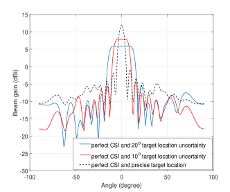
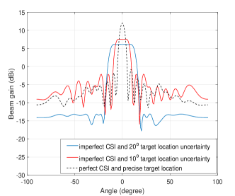
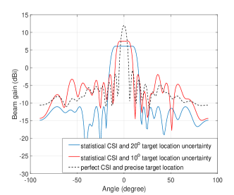
Figure 2: Beampatterns with various target direction uncertainty interval when (a) CSI is known, (b) CSI is imperfectly known and (c) statistical CSI is imperfectly known.

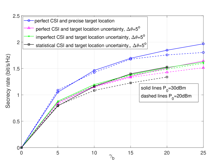
Figure 3: Achievable secrecy rate versus the threshold of SINR at legitimate users, with various transmission power budget, where solid and dashed lines represent power budget $P_{0}=30$dBm and $P_{0}=20$dBm respectively, $N=18,K=4,\Delta\theta=5^{\circ}$.

VII Numerical Results

To evaluate the proposed methods, numerical results based on Monte Carlo simulations are shown in this section to validate the effectiveness of the proposed beamforming method. Without loss of generality, each entry of channel matrix $\mathbf{H}$ is assumed to obey standard Complex Gaussian distribution, i.e. ${h_{i,j}}\sim\mathcal{C}\mathcal{N}\left({0,1}\right)$. We assume that the DFRC base station employs a ULA with half-wavelength spacing between adjacent antennas. In the following simulations, the number of antennas is set as $N=18$ and the number of legitimate users is $K=4$. The constrained beamforming design problems in Section II-Section V are solved by the classic SDR technique using the CVX toolbox [45].

VII-A Beam Gain And Secrecy Rate Analysis

We first show the resultant radar beampattern in Fig. 2 with different angular interval of target location uncertainty, i.e. $\left[{-{5^{\circ}},{5^{\circ}}}\right]$ and $\left[{-{10^{\circ}},{10^{\circ}}}\right]$. The SINR threshold of each legitimate user is set as $\gamma_{b}=10\text{dB}$. The narrow beampattern when the target location is precisely known at the BS is set as a benchmark. It is found that the desired beampattern with wide main-beam is obtained by solving the proposed algorithms, which maintain the same power in the region of possible target location. Additionally, it is noted that with the expansion of location uncertainty angular interval, the power gain of main-beam reduces.
The achievable secrecy rate in terms of increasing SINR threshold of each user is demonstrated in Fig. 3, where the power budget is set as $P_{0}=20\text{dBm}$ and $P_{0}=30\text{dBm}$ respectively. In this case, we set the sidelobe power threshold $\gamma_{s}=40\text{dB}$. Basically, in the $\text{SINR}_{E}$ minimization problem, the secrecy rate increases with the growth of $\gamma_{b}$. It is noteworthy that the system achieves higher secrecy rate when both the target location and CSI are precisely known. Besides, when we increase the power budget, the secrecy rate grows to some extent.

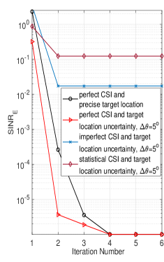
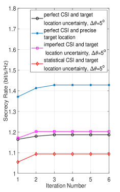
Figure 4: Convergence of (a) SINR of Eve and (b) secrecy rate for the target SINR minimization algorithm, $N=18,K=4,P_{0}=30\text{dBm},\gamma_{b}=10\text{dB}$.

In Fig. 4, we evaluate the convergence of target SINR and secrecy rate. In these cases, the same system parameters are set as previous simulations. In Fig. 4(a), the SINR of the target is confirmed to convergent to a minimum. In robust beamforming design problems, the SINR of target decreases slightly with the increasing iteration number, which results in the slight growth of secrecy rate as is shown in Fig. 4(b).

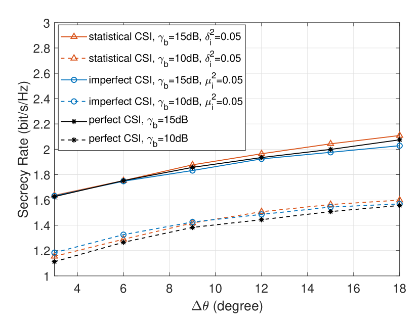
Figure 5: Secrecy rate with different angular intervals, $N=18,K=4,P_{0}=30\text{dBm}$, with $\gamma_{b}=10\text{dB}$ and $\gamma_{b}=15\text{dB}$, respectively.

VII-B Trade-off Between The Performance Of Radar And Communication System

In this subsection, we evaluate the performance trade-off between radar and communication system. Fig. 5 shows the secrecy rate performance with various angular intervals for $\gamma_{b}=10\text{dB}$ and $\gamma_{b}=15\text{dB}$. The main-beam power decreases when the target uncertainty increases, then the leaking information would get less, which improve the secrecy rate. As is demonstrated in Fig. 5, the secrecy rate increases with the growth of target uncertainty interval. Besides, with $5\text{dB}$ growth of legitimate user SINR threshold, the secrecy rate increases $0.5\text{bit/s/Hz}$ approximately.
Fig. 6 demonstrates the secrecy rate performance versus the threshold of sidelobe with $P_{0}=30\text{dBm},\Delta\theta=5^{\circ}$, which reveals the trade-off between the performance of radar and communication systems. In Algorithm 2, the power difference between main beam and sidelobe increases with the growth of $\gamma_{s}$, which results in the increasing possibility of information leaking. As the numerical result shown in Fig. 6, it is notable that the secrecy rate decreases with the growth of $\gamma_{s}$, especially the tendency gets obvious when $\gamma_{s}$ is greater than 30dB.

Figure 6: Achievable secrecy rate versus the sidelobe power with various SINR threshold of legitimate users for the Algorithm 2, $N=18,K=4,P_{0}=30\text{dBm},\Delta\theta=5^{\circ}$.

VII-C Robust Beamforming Performance

As the norm of CSI error is bounded by a constant, the secrecy rate performance versus error bound is illustrated in Fig. 7, with different location uncertainty. With the growth of error bound, the achievable SINR at each legitimate user keeps being above the given threshold but not a constant according to constraints (24c) and (27b). We note that the achievable secrecy rate reduces after a certain value with the increasing error bound, because of the different changing rate between target SINR and user SINR corresponding to various error bounds in Fig. 7. Whereas, as is shown in Fig. 8, the secrecy rate keeps increasing with the growth of error bound. In addition, the robust beamforming designs achieve higher secrecy rate when the location uncertainty is limited in a larger interval.

Figure 7: Achieved secrecy rate with different error bounds in the scenario of known imperfect CSI, $N=18,K=4,P_{0}=30\text{dBm}$.

Figure 8: Achieved secrecy rate versus different error bounds when statistical CSI is imperfectly known, $N=18,K=4,P_{0}=30\text{dBm},\gamma_{b}=10\text{dB}$.

VIII Conclusion

In this paper, optimization based beamforming designs have been addressed for MIMO DFRC system, which aimed at ensuring the security of information transmission in case of leaking to targets by adding AN at the transmitter to confuse the potential eavesdropper. Specifically, we have minimized the SINR of the target which is regarded as the potential eavesdropper while keeping the each legitimate user’s SINR above a certain constant to ensure the secrecy rate of the DFRC system. Throughout this paper, the optimization beamforming problem has been designed with perfect CSI and imperfect CSI, as well as with the accurate and inaccurate target location information.
First of all, both precise location of target and perfect CSI have been assumed to be known at BS, which gained the highest secrecy rate according to the numerical results. When the target location was uncertain, the main-beam power has decreased with the growth of the uncertainty angular interval. Moreover, the secrecy rate versus different thresholds of sidelobe has been demonstrated, which revealed the trade-off between radar and communication system performance. Then, we have formulated target SINR minimization problem with imperfect instantaneous CSI and statistical CSI known to the base station respectively. As shown in the numerical results, the beamforming design has been feasible in both robust scenarios. Finally, simulation results have been presented to show the secrecy rate tendency effected by error bound with various target location uncertainty.

References

• [1] D. Oyediran, “Spectrum sharing: Overview and challenges of small cells innovation in the proposed 3.5 GHz band.”   International Foundation for Telemetering, 2015.
• [2] B. Li, A. P. Petropulu, and W. Trappe, “Optimum co-design for spectrum sharing between matrix completion based MIMO radars and a MIMO communication system,” IEEE Transactions on Signal Processing, vol. 64, no. 17, pp. 4562–4575, 2016.
• [3] A. Ghasemi and E. S. Sousa, “Collaborative spectrum sensing for opportunistic access in fading environments,” in First IEEE International Symposium on New Frontiers in Dynamic Spectrum Access Networks, 2005. DySPAN 2005., Nov 2005, pp. 131–136.
• [4] C. W. Kim, J. Ryoo, and M. M. Buddhikot, “Design and implementation of an end-to-end architecture for 3.5 GHz shared spectrum,” in 2015 IEEE International Symposium on Dynamic Spectrum Access Networks (DySPAN).   IEEE, 2015, pp. 23–34.
• [5] G. Staple and K. Werbach, “The end of spectrum scarcity [spectrum allocation and utilization],” IEEE spectrum, vol. 41, no. 3, pp. 48–52, 2004.
• [6] S. Sodagari, A. Khawar, T. C. Clancy, and R. McGwier, “A projection based approach for radar and telecommunication systems coexistence,” in 2012 IEEE Global Communications Conference (GLOBECOM).   IEEE, 2012, pp. 5010–5014.
• [7] A. Turlapaty and Y. Jin, “A joint design of transmit waveforms for radar and communications systems in coexistence,” in 2014 IEEE Radar Conference.   IEEE, 2014, pp. 0315–0319.
• [8] B. Li and A. P. Petropulu, “Joint transmit designs for coexistence of MIMO wireless communications and sparse sensing radars in clutter,” IEEE Transactions on Aerospace and Electronic Systems, vol. 53, no. 6, pp. 2846–2864, 2017.
• [9] F. Liu, C. Masouros, A. Li, H. Sun, and L. Hanzo, “MU-MIMO communications with MIMO radar: From co-existence to joint transmission,” IEEE Transactions on Wireless Communications, vol. 17, no. 4, pp. 2755–2770, April 2018.
• [10] F. Liu, C. Masouros, A. Li, and T. Ratnarajah, “Robust MIMO beamforming for cellular and radar coexistence,” IEEE Wireless Communications Letters, vol. 6, no. 3, pp. 374–377, 2017.
• [11] F. Liu, C. Masouros, A. Li, T. Ratnarajah, and J. Zhou, “Mimo radar and cellular coexistence: A power-efficient approach enabled by interference exploitation,” IEEE Transactions on Signal Processing, vol. 66, no. 14, pp. 3681–3695, 2018.
• [12] F. Liu, L. Zhou, C. Masouros, A. Li, W. Luo, and A. Petropulu, “Toward dual-functional radar-communication systems: Optimal waveform design,” IEEE Transactions on Signal Processing, vol. 66, no. 16, pp. 4264–4279, Aug 2018.
• [13] F. Liu, L. Zhou, C. Masouros, A. Lit, W. Luo, and A. Petropulu, “Dual-functional cellular and radar transmission: Beyond coexistence,” in 2018 IEEE 19th International Workshop on Signal Processing Advances in Wireless Communications (SPAWC).   IEEE, 2018, pp. 1–5.
• [14] L. Zhou, F. Liu, C. Tian, C. Masouros, A. Li, W. Jiang, and W. Luo, “Optimal waveform design for dual-functional MIMO radar-communication systems,” in 2018 IEEE/CIC International Conference on Communications in China (ICCC).   IEEE, 2018, pp. 661–665.
• [15] A. Hassanien, M. G. Amin, Y. D. Zhang, and F. Ahmad, “Dual-function radar-communications: Information embedding using sidelobe control and waveform diversity,” IEEE Transactions on Signal Processing, vol. 64, no. 8, pp. 2168–2181, 2016.
• [16] V. Va, T. Shimizu, G. Bansal, R. W. Heath Jr et al., “Millimeter wave vehicular communications: A survey,” Foundations and Trends® in Networking, vol. 10, no. 1, pp. 1–113, 2016.
• [17] C.-H. Lim, Y. Wan, B.-P. Ng, and C.-M. S. See, “A real-time indoor wifi localization system utilizing smart antennas,” IEEE Transactions on Consumer Electronics, vol. 53, no. 2, pp. 618–622, 2007.
• [18] G. M. Dillard, M. Reuter, J. Zeiddler, and B. Zeidler, “Cyclic code shift keying: a low probability of intercept communication technique,” IEEE Transactions on Aerospace and Electronic Systems, vol. 39, no. 3, pp. 786–798, 2003.
• [19] P. M. McCormick, B. Ravenscroft, S. D. Blunt, A. J. Duly, and J. G. Metcalf, “Simultaneous radar and communication emissions from a common aperture, part ii: experimentation,” in 2017 IEEE Radar Conference (RadarConf).   IEEE, 2017, pp. 1697–1702.
• [20] W.-C. Liao, T.-H. Chang, W.-K. Ma, and C.-Y. Chi, “QoS-based transmit beamforming in the presence of eavesdroppers: An optimized artificial-noise-aided approach,” IEEE Transactions on Signal Processing, vol. 59, no. 3, pp. 1202–1216, 2011.
• [21] S. Shafiee, N. Liu, and S. Ulukus, “Towards the secrecy capacity of the Gaussian MIMO wire-tap channel: The 2-2-1 channel,” arXiv preprint arXiv:0709.3541, 2007.
• [22] F. Oggier and B. Hassibi, “The secrecy capacity of the MIMO wiretap channel,” arXiv preprint arXiv:0710.1920, 2007.
• [23] E. Ekrem and S. Ulukus, “The secrecy capacity region of the Gaussian MIMO multi-receiver wiretap channel,” IEEE Transactions on Information Theory, vol. 57, no. 4, pp. 2083–2114, 2011.
• [24] S. Goel and R. Negi, “Guaranteeing secrecy using artificial noise,” IEEE transactions on wireless communications, vol. 7, no. 6, pp. 2180–2189, 2008.
• [25] R. Negi and S. Goel, “Secret communication using artificial noise,” in IEEE Vehicular Technology Conference, vol. 62, no. 3.   Citeseer, 2005, p. 1906.
• [26] X. Zhang, X. Zhou, and M. R. McKay, “On the design of artificial-noise-aided secure multi-antenna transmission in slow fading channels,” IEEE Transactions on Vehicular Technology, vol. 62, no. 5, pp. 2170–2181, 2013.
• [27] J. P. Vilela, M. Bloch, J. Barros, and S. W. McLaughlin, “Wireless secrecy regions with friendly jamming,” IEEE Transactions on Information Forensics and Security, vol. 6, no. 2, pp. 256–266, June 2011.
• [28] Z. Chu, K. Cumanan, Z. Ding, M. Johnston, and S. Y. Le Goff, “Secrecy rate optimizations for a MIMO secrecy channel with a cooperative jammer,” IEEE Transactions on Vehicular Technology, vol. 64, no. 5, pp. 1833–1847, 2015.
• [29] P. R. Vaka, S. Bhattarai, and J.-M. Park, “Location privacy of non-stationary incumbent systems in spectrum sharing,” in 2016 IEEE Global Communications Conference (GLOBECOM).   IEEE, 2016, pp. 1–6.
• [30] A. Dimas, B. Li, M. Clark, K. Psounis, and A. Petropulu, “Spectrum sharing between radar and communication systems: Can the privacy of the radar be preserved?” in 2017 51st Asilomar Conference on Signals, Systems, and Computers.   IEEE, 2017, pp. 1285–1289.
• [31] A. Deligiannis, A. Daniyan, S. Lambotharan, and J. A. Chambers, “Secrecy rate optimizations for MIMO communication radar,” IEEE Transactions on Aerospace and Electronic Systems, vol. 54, no. 5, pp. 2481–2492, 2018.
• [32] B. K. Chalise and M. G. Amin, “Performance tradeoff in a unified system of communications and passive radar: A secrecy capacity approach,” Digital Signal Processing, vol. 82, pp. 282–293, 2018.
• [33] K. Shen and W. Yu, “Fractional programming for communication systems part i: Power control and beamforming,” IEEE Transactions on Signal Processing, vol. 66, no. 10, pp. 2616–2630, May 2018.
• [34] I. Wajid, Y. C. Eldar, and A. Gershman, “Robust downlink beamforming using covariance channel state information,” in 2009 IEEE International Conference on Acoustics, Speech and Signal Processing.   IEEE, 2009, pp. 2285–2288.
• [35] E. Telatar, “Capacity of multi-antenna Gaussian channels,” European Transactions on Telecommunications, vol. 10, no. 6, pp. 585–595. [Online]. Available: https://onlinelibrary.wiley.com/doi/abs/10.1002/ett.4460100604
• [36] K. Cumanan, Z. Ding, B. Sharif, G. Y. Tian, and K. K. Leung, “Secrecy rate optimizations for a MIMO secrecy channel with a multiple-antenna eavesdropper,” IEEE Transactions on Vehicular Technology, vol. 63, no. 4, pp. 1678–1690, May 2014.
• [37] D. R. Fuhrmann and G. San Antonio, “Transmit beamforming for MIMO radar systems using signal cross-correlation,” IEEE Transactions on Aerospace and Electronic Systems, vol. 44, no. 1, pp. 171–186, January 2008.
• [38] W. Dinkelbach, “On nonlinear fractional programming,” Management science, vol. 13, no. 7, pp. 492–498, 1967.
• [39] K.-Y. Wang, A. M.-C. So, T.-H. Chang, W.-K. Ma, and C.-Y. Chi, “Outage constrained robust transmit optimization for multiuser MISO downlinks: Tractable approximations by conic optimization,” IEEE Transactions on Signal Processing, vol. 62, no. 21, pp. 5690–5705, 2014.
• [40] M. S. Lobo, L. Vandenberghe, S. Boyd, and H. Lebret, “Applications of second-order cone programming,” Linear algebra and its applications, vol. 284, no. 1-3, pp. 193–228, 1998.
• [41] J. Li and P. Stoica, “MIMO radar with colocated antennas,” IEEE Signal Processing Magazine, vol. 24, no. 5, pp. 106–114, Sep. 2007.
• [42] F. Wang, X. Wang, and Y. Zhu, “Transmit beamforming for multiuser downlink with per-antenna power constraints,” in 2014 IEEE International Conference on Communications (ICC), June 2014, pp. 4692–4697.
• [43] A. Zappone, P. Cao, and E. A. Jorswieck, “Energy efficiency optimization in relay-assisted MIMO systems with perfect and statistical CSI,” IEEE Transactions on Signal Processing, vol. 62, no. 2, pp. 443–457, Jan 2014.
• [44] K. L. Law, I. Wajid, and M. Pesavento, “Optimal downlink beamforming for statistical CSI with robustness to estimation errors,” Signal Processing, vol. 131, pp. 472–482, 2017.
• [45] M. Grant, S. Boyd, and Y. Ye, “Cvx: Matlab software for disciplined convex programming,” 2008.