Robust pricing and hedging of options on multiple assets and its numerics

Abstract

We consider robust pricing and hedging for options written on multiple assets given market option prices for the individual assets. The resulting problem is called the multi-marginal martingale optimal transport problem. We propose two numerical methods to solve such problems: using discretisation and linear programming applied to the primal side and using penalisation and deep neural networks optimisation applied to the dual side. We prove convergence for our methods and compare their numerical performance. We show how adding further information about call option prices at additional maturities can be incorporated and narrows down the no-arbitrage pricing bounds. Finally, we obtain structural results for the case of the payoff given by a weighted sum of covariances between the assets.

forthcoming in SIAM Journal on Financial Mathematics

60G42, 49M25, 49M29, 90C08

1 Introduction

Mathematical modelling is a ubiquitous aspect of modern the financial industry and it drives important decision processes. Stochastic models are a key component used to describe evolution of risky assets and quantify financial risks. The ability to postulate and analyse such models was at the heart of the growth in ever more complex derivatives trading and other aspects of the financial markets. However, understanding well the implications of a given model is not sufficient. Equally important is to appreciate the consequences of the model being wrong in the sense of being an inadequate or misguided description of the reality. The latter issue is often referred to as the Knightian uncertainty after Knight, (1921). This dichotomy between risk and uncertainty, and the quest to capture both and understand their interplay, are at the heart of the field of Robust Mathematical Finance. The field is concerned with the modelling space, from model-free to model-specific approaches, and with understanding and quantifying the impact of making assumptions, and of using or ignoring market information. It has been an important area of research, in particular in the last decade following the financial crisis, and we refer to Burzoni et al., (2019) and the references therein for an extensive discussion. One of the most active research topics within the field has been that of model-independent pricing and hedging of derivatives. It goes back to Hobson, (1998) and probabilistic methods related to Skorokhod embeddings, see for example Brown et al., (2001); Cox and Obłój, (2011). More recently, it has been recast as an optimal transport problem with a martingale constraint, see Beiglböck et al., (2013); Galichon et al., (2014) and gained a novel momentum. A significant body of research grew studying this Martingale Optimal Transport (MOT) problem both in discrete and continuous time, see for example Beiglböck et al., 2017a ; Beiglböck et al., 2017b ; Dolinsky and Soner, (2014); Hou and Obłój, (2018) and the references therein. More recently, first numerical methods for MOT problems were developed in Guo and Obłój, (2019); Eckstein and Kupper, (2019). However, all these works assume that markets provide sufficient information to derive the joint, multi-dimensional, risk neutral distribution of assets at given maturities. In dimensions greater than one, this assumption is unrealistic in most markets.

In contrast, in this paper, we propose to study problems, in dimensions greater than one, which are directly motivated by typical market settings and the available market data. Our focus is on numerical methods and we aim to deliver a proof-of-concept results which, we hope, could spark interest in these methods among industry practitioners. More precisely, we assume market prices of call and put options are given for individual assets - these could be for one or many maturities. For simplicity, we focus on the case when such prices are given for enough strikes to derive the implied risk-neutral distribution, a standard argument going back to Breeden and Litzenberger, (1978). Our numerical methods can easily be adjusted to the case of only finitely many traded call options and we establish a continuity result to justify our focus on the synthetic limiting case. Given the market information, we study the implied no-arbitrage bounds for an option with a payoff which depends on multiple assets. A simple example, with two assets, is given by a spread option. In higher dimensions, natural examples are given by options written on an index. We stress that while market information translates into risk neutral distributional constraints on individual assets, the global no-arbitrage constraint translates into a global martingale constraint which binds the assets together and is sharper than just requiring that each of the assets were a martingale in its own filtration.

We call the resulting optimisation problem a Multi-Marginal Martingale Optimal Transport (MMOT) problem. It was first studied in Lim, (2016) who focused on its duality theory. The duality is of intrinsic financial interest: while the primal problem corresponds to the risk-neutral pricing, the dual side corresponds to optimising over hedging strategies. The equality between the primal and the dual problem corresponds to the superhedging duality in mathematical finance. We exploit it here to propose two different numerical methods for MMOT problems. First, we adopt the approach of Guo and Obłój, (2019) and propose a computational method for the primal problem. This relies on discretisation of the marginal measures combined with a relaxation of the martingale condition. Theorem 3.1 establishes convergence of the approximating problems to the original MMOT problem. Each approximating problem in turn, is a discrete LP problem and can be solved efficiently. The main disadvantage of this approach is the curse of dimensionality: LP problems with too many constraints quickly exceed memory capacity. Our second approach builds on the work of Eckstein and Kupper, (2019) to develop a computational method for solving the dual problem. The dual problem involves an optimisation over hedging strategies and we approximate these with elements of a deep neural network (NN). To employ the stochastic gradient descent we change the problem from a singular one, with the superhedging inequality constraint, to a smooth one with an integral penalty term. Theorem 3.7 shows that under suitable assumptions the results converge, with the penalty term $\gamma\to\infty$ and the size of the NN $m\to\infty$, to the value of the MMOT problem.

The numerical methods we propose, including Theorems 3.1 and 3.7, are natural extensions of the previous MOT studies cited above and do not require fundamental new insights. In this way, our results illustrate that these studies are generic in nature and can be extended or generalised to other similar contexts. Apart from the MMOT problem studied here, we mention the optimization problem considered by Kramkov and Xu, (2019). A large focus of our paper then lies on making the method practically applicable and testing their numerical performance. We discuss the details of the implementation and provide GitHub links with the codes. We show that the NN approach agrees with the LP approach but is also able to handle higher dimensional settings. Both approaches are shown to recover theoretical values, when these can be computed independently. By focusing on a MMOT problem which corresponds to real world industry scenarios we hope to showcase the capacity of the robust approach to capture and quantify, in a fully non-parametric and model-agnostic way, the impact of various sources of information, or ways to trade, for a given pricing and hedging problem. We illustrate this on both synthetic and real world data. In particular, we consider the case of payoffs only depending on the assets’ terminal values at time $T$, e.g., spread options and options paying covariance between the assets. Such examples allow us to capture the value of additional market information from intermediate maturities. Indeed, we can start by considering only the call prices at time $T$, i.e., MMOT becomes just an optimal transport problem, or the so-called robust copula, see for example Wang et al., (2013). Adding call prices at earlier maturities $T_{i}<T$ then reduces the range of no-arbitrage prices and thus captures the value of this information for robust pricing and hedging. This, along with the structure of optimisers, can be understood and characterised theoretically as Theorem 5.3 shows.

The remainder of this paper is structured as follows. In Section 2 we introduce the MMOT problem and its duality. Then we develop our computational methods: first the LP approach in Section 3.1 and then the NN approach in Section 3.2. All the numerical examples are presented in the subsequent Section 4. Finally, in Section 5, we discuss some structural results for the particular case of the covariance payoff.

2 The MMOT problem

We denote by ${\mathcal{P}}(\mathbb{R}^{d})$ the set of probability measures on $\mathbb{R}^{d}$ with a finite first moment. Measurable (resp. continuous) functions from $\mathbb{R}^{d}$ to $\mathbb{R}^{k}$ are denoted $\mathbf{L}^{0}(\mathbb{R}^{d};\mathbb{R}^{k})$ (resp. $C(\mathbb{R}^{d};\mathbb{R}^{k})$) and we write $C_{b}$ for continuous bounded functions. For a $\mu\in{\mathcal{P}}(\mathbb{R}^{d})$, $\mathbf{L}^{1}(\mu)$ denotes the space of functions $f:\mathbb{R}^{d}\to\mathbb{R}$ with $\int|f|d\mu<\infty$.

Let $T,d\in\mathbb{N}$ and ${\mathcal{X}}_{1}={\mathcal{X}}_{2}=...={\mathcal{X}}_{T}=\mathbb{R}^{d}$, ${\mathcal{X}}={\mathcal{X}}_{1}\times...\times{\mathcal{X}}_{T}$. We denote the natural projection from ${\mathcal{X}}$ onto its $t^{\textrm{th}}$ component by $X_{t}$, and by $X_{t,i}$ the further projection onto the $i$-th component of ${\mathcal{X}}_{t}$. For $x\in{\mathcal{X}}$ we write $x_{t}=X_{t}(x)$ and $x_{t,i}=X_{t,i}(x)$. Given $\mu_{t,i}\in{\mathcal{P}}(\mathbb{R})$, let $\check{\mu}_{t}=(\mu_{t,i})_{1\leq i\leq d}$ and $\check{\mu}=(\check{\mu}_{t})_{1\leq t\leq T}$. We define $\Pi(\check{\mu})=\Pi(\check{\mu}_{1},...,\check{\mu}_{T})\subset{\mathcal{P}}({\mathcal{X}})$ as the set of measures $\pi$ satisfying $\pi\circ X_{t,i}^{-1}=\mu_{t,i}$ for $1\leq t\leq T$ and $1\leq i\leq d$. We stress that throughout we only consider measures with a finite first moment.

We assume from now onwards that $\mu_{t,i}$ are increasing in convex order in $t$, denoted $\mu_{t,i}\preceq_{cx}\mu_{t+1,i}$, by which we mean that

$$\int fd\mu_{t,i}\leq\int fd\mu_{t+1,i}\quad\text{for all convex functions }f,\;\;1\leq t\leq T-1,1\leq i\leq d.$$

We define $\mathcal{M}(\check{\mu})=\mathcal{M}(\check{\mu}_{1},...,\check{\mu}_{T})\subseteq\Pi(\check{\mu})$ to be the subset consisting of martingale measures, i.e., measures $\pi$ such that

$$\mathbb{E}_{\pi}[X_{t+1}|X_{1},...,X_{t}]=X_{t},\quad 1\leq t\leq T-1.$$

It follows from Strassen, (1965) that our increasing convex order assumptions on $\check{\mu}$ are precisely the necessary and sufficient conditions for $\mathcal{M}(\check{\mu})\neq\emptyset$.

Our object of interest in this paper is the multi-marginal martingale optimal transport (MMOT) defined as

(1) $$\begin{split}\overline{\mathsf{MMOT}}(\check{\mu})\quad&:=\quad\overline{\mathsf{P}}(\check{\mu})\quad:=\quad\sup_{\pi\in\mathcal{M}(\check{\mu})}\leavevmode\nobreak\ \int c\,d\pi,\\ \underline{\mathsf{MMOT}}(\check{\mu})\quad&:=\quad\underline{\mathsf{P}}(\check{\mu})\quad:=\quad\inf_{\pi\in\mathcal{M}(\check{\mu})}\leavevmode\nobreak\ \int c\,d\pi,\end{split}$$

for a given measurable function $c:{\mathcal{X}}\to\mathbb{R}$ to optimize. We recall that the martingale condition encodes the financial requirement of absence of arbitrage. We mostly use the notation $\overline{\mathsf{P}},\underline{\mathsf{P}}$. However when we want to stress the martingale condition, we write $\overline{\mathsf{MMOT}},\underline{\mathsf{MMOT}}$. Without this condition, the problem above corresponds to the multi-marginal optimal transport, given by

(2) $$\begin{split}\overline{\mathsf{OT}}(\check{\mu})\quad&:=\quad\sup_{\pi\in\Pi(\check{\mu})}\leavevmode\nobreak\ \int c\,d\pi,\\ \underline{\mathsf{OT}}(\check{\mu})\quad&:=\quad\inf_{\pi\in\Pi(\check{\mu})}\leavevmode\nobreak\ \int c\,d\pi.\end{split}$$

In the particular case when $d=2$ and $c(x)=c(x_{T,1},x_{T,2})$ the above corresponds to the classical optimal transport problem on $\mathbb{R}$ as only the marginals $\mu_{T,i}$, $i=1,2$, impact the problem. The case $c(x)=|x_{T,1}-x_{T,2}|$ gives $\underline{\mathsf{OT}}(\check{\mu})={\mathcal{W}}_{1}(\mu_{T,1},\mu_{T,2})$, which is the Wasserstein distance of order $1$, a metric on ${\mathcal{P}}(\mathbb{R})$ which we will use extensively in Section 3.1. Note that in general

$$\underline{\mathsf{OT}}\leqslant\underline{\mathsf{MMOT}}\leqslant\overline{\mathsf{MMOT}}\leqslant\overline{\mathsf{OT}}.$$

Both problems (1) and (2) admit a dual formulation. The latter can be found in Bartl et al., (2017), while the former was developed in Lim, (2016), following earlier works on the martingale optimal transport in Beiglböck et al., (2013). We recall it here as it will be used for our numerical methods. Define $\overline{{\mathcal{D}}}$, respectively $\underline{{\mathcal{D}}}$, to be the set of functions $(\varphi_{t,i})_{1\leq t\leq T,1\leq i\leq d}$ and $(h_{t,i})_{1\leq t\leq T-1,1\leq i\leq d}$, where $\varphi_{t,i}\in\mathbf{L}^{1}(\mu_{t,i})$ and $h_{t,i}\in\mathbf{L}^{0}(\mathbb{R}^{t\cdot d};\mathbb{R})$, satisfying for all $x\in{\mathcal{X}}$:

$$\sum_{t=1}^{T}\sum_{i=1}^{d}\varphi_{t,i}(x_{t,i})+\sum_{t=1}^{T-1}\sum_{i=1}^{d}h_{t,i}(x_{1},...,x_{t})(x_{t+1,i}-x_{t,i}) \geq c(x),\quad\text{respectively}$$

$$\sum_{t=1}^{T}\sum_{i=1}^{d}\varphi_{t,i}(x_{t,i})+\sum_{t=1}^{T-1}\sum_{i=1}^{d}h_{t,i}(x_{1},...,x_{t})(x_{t+1,i}-x_{t,i}) \leq c(x).$$

Then the corresponding dual problems are defined by

(3) $$\begin{split}\overline{\mathsf{D}}(\check{\mu})\quad:=&\quad\inf_{(\varphi_{t,i},h_{t,i})\in\overline{{\mathcal{D}}}}\leavevmode\nobreak\ \sum_{t=1}^{T}\sum_{i=1}^{d}\int\varphi_{t,i}\,d\mu_{t,i},\\ \underline{\mathsf{D}}(\check{\mu})\quad:=&\quad\sup_{(\varphi_{t,i},h_{t,i})\in\underline{{\mathcal{D}}}}\leavevmode\nobreak\ \sum_{t=1}^{T}\sum_{i=1}^{d}\int\varphi_{t,i}\,d\mu_{t,i}.\end{split}$$

Let us now discuss briefly the financial interpretation of the objects introduced so far. We refer the reader to Beiglböck et al., (2013); Burzoni et al., (2019) and the references therein for more details and for background on robust financial mathematics. We consider a market with $d$ traded risky assets and $T$ time steps, or maturities. All prices are discounted, i.e., given in units of a fixed numeraire (e.g., the bank account). The price of $i^{\textrm{th}}$ asset at $t^{\mathrm{th}}$ maturity is denoted $x_{t,i}$ above. We suppose market provides call/put option prices for each of these assets for all $T$ maturities and all strikes. This, through a classical argument of Breeden and Litzenberger, (1978), is equivalent to fixing the risk neutral marginal distributions of the assets. We denote $\mu_{t,i}$ the risk-netural marginal distribution of $i^{\textrm{th}}$ asset at $t^{\mathrm{th}}$ maturity. In particular, the first maturity will often correspond to today and then $\mu_{1,i}=\delta_{s_{i}}$ where $s_{i}$ is today’s price of the $i^{\textrm{th}}$ asset. $\mathcal{M}(\check{\mu})$ is the set of all risk neutral (i.e., martingale) measures for the whole market which are calibrated to the given option prices. Thus, the primal problem (1) takes the risk-netural pricing perspective and gives the upper and lower bounds for the price of a derivative with payoff $c$ at the final maturity. The dual problem (3) considers the same quantities but from the hedging perspective. Here, $\varphi_{t,i}(x_{t,i})$ represents the static position synthetised from $t^{\textrm{th}}$ maturity call/put options on the $i^{\textrm{th}}$ asset and $h_{t,i}$ is the number of shares of the $i^{\textrm{th}}$ asset held between the $t^{\textrm{th}}$ and $(t+1)^{\textrm{th}}$ maturity. Importantly, $h_{t,i}$ is a function of the past prices of all assets across the previous maturities. This, on the primal side, corresponds to the requirement that the assets are jointly martingale and not just each on their own. Classically, the pricing and the hedging approach should give the same no-arbitrage price range. This is also the case here as stated in the following theorem.

Theorem 2.1.

Let $\check{\mu}\in{\mathcal{P}}(\mathbb{R})^{dT}$ with $\mathcal{M}(\check{\mu})\neq\emptyset$, and let $\psi:{\mathcal{X}}\rightarrow\mathbb{R}$ be given by $\psi(x)=1+\sum_{t=1}^{T}\sum_{i=1}^{d}|x_{t,i}|$. If $c:{\mathcal{X}}\to\mathbb{R}$ is lower semi-continuous and $c\geq-K\psi$ on ${\mathcal{X}}$ for some $K>0$ then $\underline{\mathsf{P}}(\check{\mu})=\underline{\mathsf{D}}(\check{\mu})$. If $c:{\mathcal{X}}\to\mathbb{R}$ is upper semi-continuous and $c\leq K\psi$ on ${\mathcal{X}}$ for some $K>0$ then $\overline{\mathsf{P}}(\check{\mu})=\overline{\mathsf{D}}(\check{\mu})$. In both cases, the primal problems are attained and the dual values remain unchanged when one restricts to $\varphi_{t,i}\in\mathbf{L}^{1}(\mu_{t,i})\cap C(\mathbb{R};\mathbb{R})$, $h_{t,i}\in C_{b}(\mathbb{R}^{t\cdot d};\mathbb{R}^{d})$, $1\leq t\leq T$, $1\leq i\leq d$.

We note that this result was proved in Zaev, (2015) with the assumption of continuous cost $c$, but it is standard to extend the duality to the semi-continuous costs, see, e.g., Villani, (2003, 2009). We also note that this duality for martingale optimal transport was first proved in Beiglböck et al., (2013) in one dimension $d=1$, and they also showed that the duality holds with a narrower class of functions $\varphi_{t,i}$ which are linear combinations of finitely many call options, i.e. $\varphi_{t,i}$ of the form $c_{t,i}+\sum_{j=i}^{l_{t,i}}c_{t,i,j}(x_{t,i}-k_{t,i,j})^{+}$, for some $l_{\cdot},c_{\cdot},k_{\cdot}$. The same applies here.

While existence of primal optimizers in (1) is easy to obtain, in general we cannot hope for uniqueness. We illustrate this with two simple examples. In both examples, $d=2=T$ and $c(x)=x_{2,1}x_{2,2}$. We further study this particular cost function and present some structural results in Section 5.

Example 2.2.

Consider $d=2=T$ and the maximization problem with $c(x)=x_{2,1}x_{2,2}$. Take $\mu\preceq_{cx}\nu$ such that $\mathcal{M}(\mu,\nu)$ is not a singleton, e.g., $\mu,\nu$ are Gaussians with the same mean and increasing variance, and let $\mu_{1,1}=\mu_{1,2}=\mu$, $\mu_{2,1}=\mu_{2,2}=\nu$. Then for any $\tilde{\pi}\in\mathcal{M}(\mu,\nu)$, the distribution $\pi$ of any quadruple of random variables $(\xi,\xi,\eta,\eta)$ satisfying $(\xi,\eta)\sim\tilde{\pi}$ is an element of $\mathcal{M}(\check{\mu})$. Further, $\pi\circ X_{2}^{-1}$ is the monotone increasing coupling of $\nu$ with itself and, in particular, is independent of the choice of $\tilde{\pi}$. It also attains $\overline{\mathsf{P}}(\check{\mu})$ and we conclude that the optimizer in $\overline{\mathsf{P}}(\check{\mu})$ is not unique. Note however that, in this example, the distributions $\pi\circ X_{1}^{-1}$ and $\pi\circ X_{2}^{-1}$ are the same for any optimizer $\pi\in\mathcal{M}(\check{\mu})$.

Example 2.3.

Consider the same problem as in Example 2.2 but with $\mu_{1,1}=\delta_{0}$, $\mu_{2,1}=\frac{1}{4}(\delta_{-2}+\delta_{-1}+\delta_{1}+\delta_{2})$, $\mu_{1,2}=\mu_{2,2}=\frac{1}{2}(\delta_{-1}+\delta_{1})$. Note that, for any $\pi\in\mathcal{M}(\check{\mu})$, $\pi^{1}=\pi\circ X_{1}^{-1}=\frac{1}{2}(\delta_{(0,1)}+\delta_{(0,-1)})$. Further, the following measures dominate $\pi^{1}$ in the convex order and have $\mu_{2,1},\mu_{2,2}$ as their marginals:

$$\pi^{2}=\frac{1}{4}(\delta_{(-1,1)}+\delta_{(1,1)}+\delta_{(-2,-1)}+\delta_{(2,-1)}),$$

$$\tilde{\pi}^{2}=\frac{1}{4}(\delta_{(-1,-1)}+\delta_{(1,-1)}+\delta_{(-2,1)}+\delta_{(2,1)}).$$

Hence there exist $\pi,\tilde{\pi}\in\mathcal{M}(\check{\mu})$ whose (2-dimensional) marginals are $\pi^{1},\pi^{2}$ and $\pi^{1},\tilde{\pi}^{2}$ respectively. In particular, $\mathcal{M}(\check{\mu})$ is not a singleton. However, for any $\pi\in\mathcal{M}(\check{\mu})$, we have

$$\mathbb{E}_{\pi}[X_{2,1}X_{2,2}]=\mathbb{E}_{\pi}[X_{2,1}X_{1,2}]=\mathbb{E}_{\pi}[X_{1,1}X_{1,2}]=0,$$

and hence $\pi$ is an optimizer for both $\underline{\mathsf{P}}(\check{\mu})$ and $\overline{\mathsf{P}}(\check{\mu})$ with $c(x)=x_{2,1}x_{2,2}$. In this example, neither the optimizer nor the implied distribution of $X_{2}$ are unique.

3 Numerical Methods for MMOT problems

We present now two numerical approaches for computing the MMOT value (1), as well as the primal and the dual optimizers. Our first approach relies on the primal formulation (1) and LP methods. Our second approach starts with the dual formulation (3), uses penalization to convexify the superhedging constraint and employs optimization techniques involving deep neural networks.

Before we discuss our methods in detail, we mention briefly two other numerical approaches which have been applied to MOT problems and, while not pursued in this paper, could potentially be extended to the MMOT context. The first one is the cutting plane method as described in Henry-Labordère, (2013). This method is LP based but works via the dual side. A standard LP approach runs into memory issues for higher values of $d$ or $T$, see section 4.3, and the cutting plane method circumvents this by considering a finite set of basis functions. While effective, this introduces a new source of error and one which is difficult to control theoretically and for this reason, see also section 4.1, we do not discuss it further in this paper. The second method is a generalization of the Sinkhorn algorithm Benamou et al., (2015); Cuturi, (2013) to the MOT problem, see De March, (2018). The Sinkhorn algorithm adds a strictly convex/concave term to the objective function, similarly as our neural network approach presented below. However, the Sinkhorn algorithm is designed for discrete marginals and based on the so-called iterative Bregman projections. In the OT context, the projections are onto the marginal constraints. The added difficulty for MOT problems comes from the additional projection onto the martingale constraint, which does not admit a closed form solution. Instead, the projection has to be approximated numerically, e.g., using Newton’s method, which again introduces a new source of error. To the best of our knowledge, even for MOT problems, there are no theoretical results ensuring that the accumulative error does not explode and the number of required projections does not increase with respect to the discretisation precision.

3.1 The Primal Problem - an LP approach

Following the approach of Guo and Obłój, (2019), we propose a computational scheme to solve (1). For each $\varepsilon\in\mathbb{R}_{+}$, denote by $\mathcal{M}_{\varepsilon}(\check{\mu})\subset\Pi(\check{\mu})$ the subset of measures $\pi$ satisfying

$$\mathbb{E}_{\pi}\Big{[}\Big{|}\mathbb{E}_{\pi}\big{[}X_{t+1}\big{|}X_{1},\ldots,X_{t}\big{]}\leavevmode\nobreak\ -\leavevmode\nobreak\ X_{t}\Big{|}\Big{]}\quad\leq\quad\varepsilon,\quad\mbox{ for }t=1,\ldots,T-1,$$

where $|\cdot|$ stands for the $\ell_{1}$ norm. Introduce, accordingly, the optimization problems as follows:

$$\overline{\mathsf{P}}_{\varepsilon}(\check{\mu})\quad:=\quad\sup_{\pi\in\mathcal{M}_{\varepsilon}(\check{\mu})}\leavevmode\nobreak\ \int c\,d\pi,\qquad\underline{\mathsf{P}}_{\varepsilon}(\check{\mu})\quad:=\quad\inf_{\pi\in\mathcal{M}_{\varepsilon}(\check{\mu})}\leavevmode\nobreak\ \int c\,d\pi.$$

Then clearly $\overline{\mathsf{P}}_{0}=\overline{\mathsf{P}}$ (resp. $\underline{\mathsf{P}}_{0}=\underline{\mathsf{P}}$), and Theorem 3.1 provides the basis of our numerical method.

Theorem 3.1.

Let $\check{\mu}\in{\mathcal{P}}(\mathbb{R})^{dT}$ satisfy $\mathcal{M}(\check{\mu})\neq\emptyset$ and $\check{\mu}^{n}=\big{(}\mu_{t,i}^{n}\big{)}_{1\leq t\leq T,1\leq i\leq d}$ satisfy $\lim_{n\to\infty}r_{n}=0$ with $r_{n}:=2\max_{1\leq t\leq T}\sum_{1\leq i\leq d}{\mathcal{W}}_{1}(\mu_{t,i}^{n},\mu_{t,i})$. Then, for all $n\geq 1$, $\mathcal{M}_{r_{n}}(\check{\mu}^{n})\neq\emptyset$. Assume further $c$ is Lipschitz, then:

(i)  For any $(\varepsilon_{n})_{n\geq 1}$ converging to zero such that $\varepsilon_{n}\geq r_{n}$ for all $n\geq 1$, one has

$$\lim_{n\to\infty}\overline{\mathsf{P}}_{\varepsilon_{n}}(\check{\mu}^{n})=\overline{\mathsf{P}}(\check{\mu})\mbox{ and }\lim_{n\to\infty}\underline{\mathsf{P}}_{\varepsilon_{n}}(\check{\mu}^{n})=\underline{\mathsf{P}}(\check{\mu}).$$

(ii)  For each $n\geq 1$, $\overline{\mathsf{P}}_{\varepsilon_{n}}(\check{\mu}^{n})$ (resp. $\underline{\mathsf{P}}_{\varepsilon_{n}}(\check{\mu}^{n})$) admits an optimizer $\pi_{n}$. The sequence $(\pi_{n})_{n\geq 1}$ is tight and every limit point is an optimizer for $\overline{\mathsf{P}}(\check{\mu})$ (resp. $\underline{\mathsf{P}}(\check{\mu})$). In particular, $(\pi_{n})_{n\geq 1}$ converges weakly whenever $\overline{\mathsf{P}}(\check{\mu})$ (resp. $\underline{\mathsf{P}}(\check{\mu})$) has a unique optimizer.

Before proving this result we state and prove two preliminary propositions.

Proposition 3.2.

Provided $\check{\mu}\in{\mathcal{P}}(\mathbb{R})^{dT}$ with $\mathcal{M}_{\varepsilon}(\check{\mu})\neq\emptyset$, it holds $\mathcal{M}_{\varepsilon+r}(\check{\mu}^{\prime})\neq\emptyset$ for all $\check{\mu}^{\prime}\in{\mathcal{P}}(\mathbb{R})^{dT}$ where $r:=2\max_{1\leq t\leq T}\sum_{1\leq i\leq d}{\mathcal{W}}_{1}(\mu_{t,i}^{\prime},\mu_{t,i})$. Further, if $c$ is $L-$Lipschitz, then

$$\overline{\mathsf{P}}_{\varepsilon}(\check{\mu})\leavevmode\nobreak\ \leq\leavevmode\nobreak\ \overline{\mathsf{P}}_{\varepsilon+r}(\check{\mu}^{\prime})+LTr/2\quad\text{and}\quad\underline{\mathsf{P}}_{\varepsilon}(\check{\mu})\leavevmode\nobreak\ \geq\leavevmode\nobreak\ \underline{\mathsf{P}}_{\varepsilon+r}(\check{\mu}^{\prime})-LTr/2.$$

Proof 3.3.

Without loss of generality, we only show the first inequality. Fix an arbitrary $\pi\in\mathcal{M}_{\varepsilon}(\check{\mu})$. It follows from Skorokhod’s theorem that, there exists an enlarged probability space $(E,{\mathcal{E}},{\mathcal{Q}})$ which supports random variables $U_{t}=(U_{t,1},\ldots,U_{t,d})$, $Z_{t}=(Z_{t,1},\ldots,Z_{t,d})$ taking values in $\mathbb{R}^{d}$, for $t=1,\ldots,T$, such that

(4) $$\begin{split}\leavevmode\nobreak\ \leavevmode\nobreak\ \leavevmode\nobreak\ &\text{$\bullet$\leavevmode\nobreak\ ${\mathcal{Q}}\circ(U_{1},...,U_{T})^{-1}=\pi$ and ${\mathcal{Q}}\circ Z_{t}^{-1}={\mathcal{N}}_{d}$ for $t=1,\ldots,T$,}\\ \leavevmode\nobreak\ \leavevmode\nobreak\ \leavevmode\nobreak\ &\text{where ${\mathcal{N}}_{d}$ denotes the standard normal distribution on $\mathbb{R}^{d}$.}\\ \leavevmode\nobreak\ \leavevmode\nobreak\ \leavevmode\nobreak\ &\text{$\bullet$\leavevmode\nobreak\ $(U_{1},\ldots,U_{T})$ and $(Z_{1},\ldots,Z_{T})$ are independent.}\end{split}$$

Let $t\in\{1,\ldots,T-1\}$. For $i=1,\ldots,d$, let $\gamma_{t,i}$ be the optimal transport plan realizing the Wasserstein distance ${\mathcal{W}}_{1}(\mu_{t,i},\mu_{t,i}^{\prime})$. Using standard disintegration techniques (see (Guo and Obłój,, 2019, Lemma A.1)), there exist measurable functions $f_{t,i}:\mathbb{R}^{2}\to\mathbb{R}$ such that ${\mathcal{Q}}\circ(U_{t,i},V_{t,i})^{-1}=\gamma_{t,i}$ with $V_{t,i}:=f_{t,i}(U_{t,i},Z_{t,i})$. Let $V_{t}:=(V_{t,1},\ldots,V_{t,d})$. Then, for all $h=(h_{i})_{1\leq i\leq d}\in{\mathcal{C}}_{b}\big{(}{\mathcal{X}}_{1}\times\cdots\times{\mathcal{X}}_{t};\mathbb{R}^{d}\big{)}$, one has

$$\mathbb{E}_{{\mathcal{Q}}}\big{[}h(V_{1},\ldots,V_{t})\cdot(V_{t+1}-V_{t})\big{]}\leavevmode\nobreak\ =\leavevmode\nobreak\ \mathbb{E}_{{\mathcal{Q}}}\left[\sum_{i=1}^{d}h_{i}(V_{1},\ldots,V_{t})(V_{t+1,i}-V_{t,i})\right]$$

$$=\leavevmode\nobreak\ \mathbb{E}_{{\mathcal{Q}}}\left[\sum_{i=1}^{d}h_{i}(V_{1},\ldots,V_{t})(V_{t+1,i}-U_{t+1,i})\right]\leavevmode\nobreak\ +\leavevmode\nobreak\ \mathbb{E}_{{\mathcal{Q}}}\left[\sum_{i=1}^{d}h_{i}(V_{1},\ldots,V_{t})(U_{t+1,i}-U_{t,i})\right]$$

$$\leavevmode\nobreak\ \leavevmode\nobreak\ +\leavevmode\nobreak\ \mathbb{E}_{{\mathcal{Q}}}\left[\sum_{i=1}^{d}h_{i}(V_{1},\ldots,V_{t})(U_{t,i}-V_{t,i})\right]$$

$$\leq\leavevmode\nobreak\ r\|h\|_{\infty}\leavevmode\nobreak\ +\leavevmode\nobreak\ \mathbb{E}_{{\mathcal{Q}}}\left[\sum_{i=1}^{d}h_{i}\big{(}f_{s,i}(U_{s,i},Z_{s,i});1\leq s\leq t,1\leq i\leq d\big{)}(U_{t+1,i}-U_{t,i})\right]$$

$$\leq\leavevmode\nobreak\ (\varepsilon+r)\|h\|_{\infty},$$

where the last inequality follows from the conditions in (4). Therefore,

(5) $$\int h(x_{1},\ldots,x_{t})\cdot(x_{t+1}-x_{t})\pi^{\prime}(dx)\quad\leq\quad(\varepsilon+r)\|h\|_{\infty}$$

holds for all $h\in{\mathcal{C}}_{b}\big{(}{\mathcal{X}}_{1}\times\cdots\times{\mathcal{X}}_{t};\mathbb{R}^{d}\big{)}$, where $\pi^{\prime}:={\mathcal{Q}}\circ(V_{1},\ldots,V_{T})^{-1}$. In view of the monotone class theorem, this is equivalent to

$$\mathbb{E}_{\pi^{\prime}}\Big{[}\Big{|}\mathbb{E}_{\pi^{\prime}}\big{[}X_{t+1}\big{|}X_{1},\ldots,X_{t}\big{]}\leavevmode\nobreak\ -\leavevmode\nobreak\ X_{t}\Big{|}\Big{]}\quad\leq\quad\varepsilon+r.$$

Hence, $\pi^{\prime}\in\mathcal{M}_{\varepsilon+r}(\check{\mu}^{\prime})\neq\emptyset$ as $\pi^{\prime}\circ X_{t,i}^{-1}=\mu_{t,i}^{\prime}$ for $t=1,\ldots,T$ and $i=1,\ldots,d$. To conclude the proof, notice that

$$\int cd\pi\leavevmode\nobreak\ -\leavevmode\nobreak\ \overline{\mathsf{P}}_{\varepsilon+r}(\check{\mu}^{\prime}) \leq \int cd\pi\leavevmode\nobreak\ -\leavevmode\nobreak\ \int cd\pi^{\prime}\leavevmode\nobreak\ \leavevmode\nobreak\ =\leavevmode\nobreak\ \leavevmode\nobreak\ \mathbb{E}_{{\mathcal{Q}}}\big{[}c(U_{1},\ldots,U_{T})-c(V_{1},\ldots,V_{T})\big{]}$$

$$\leq L\sum_{t=1}^{T}\sum_{i=1}^{d}\mathbb{E}_{{\mathcal{Q}}}\big{[}|U_{t,i}-V_{t,i}|\big{]}\leavevmode\nobreak\ \leavevmode\nobreak\ \leq\leavevmode\nobreak\ \leavevmode\nobreak\ LTr/2,$$

which yields $\overline{\mathsf{P}}_{\varepsilon}(\check{\mu})\leq\overline{\mathsf{P}}_{\varepsilon+r}(\check{\mu}^{\prime})+LTr/2$ as $\pi\in\mathcal{M}_{\varepsilon}(\check{\mu})$ is arbitrary.

Proposition 3.4.

Assume that $c$ has a linear growth and $\mathcal{M}(\check{\mu})\neq\emptyset$.

(i)  If $c$ is u.s.c., then the map $\mathbb{R}_{+}\ni\varepsilon\mapsto\overline{\mathsf{P}}_{\varepsilon}(\check{\mu})\in\mathbb{R}$ is non-decreasing, continuous and concave.

(ii)  If $c$ is l.s.c., then the map $\mathbb{R}_{+}\ni\varepsilon\mapsto\underline{\mathsf{P}}_{\varepsilon}(\check{\mu})\in\mathbb{R}$ is non-increasing, continuous and convex.

Proof 3.5.

We only show (i) here. First notice that $\varepsilon\mapsto\overline{\mathsf{P}}_{\varepsilon}(\check{\mu})$ is non-decreasing by definition. Next, let us prove the concavity. Given $\varepsilon$, $\varepsilon^{\prime}\in\mathbb{R}_{+}$ and $\alpha\in[0,1]$, it remains to show $(1-\alpha)\overline{\mathsf{P}}_{\varepsilon}(\check{\mu})+\alpha\overline{\mathsf{P}}_{\varepsilon^{\prime}}(\check{\mu})\leq\overline{\mathsf{P}}_{\varepsilon_{\alpha}}(\check{\mu})$, where $\varepsilon_{\alpha}:=(1-\alpha)\varepsilon+\alpha\varepsilon^{\prime}$. This indeed follows from the fact that $(1-\alpha)\pi+\alpha\pi^{\prime}\in\mathcal{M}_{\varepsilon_{\alpha}}(\check{\mu})$ for all $\pi\in\mathcal{M}_{\varepsilon}(\check{\mu})$ and $\pi^{\prime}\in\mathcal{M}_{\varepsilon^{\prime}}(\check{\mu})$. Hence the map restricted to $(0,+\infty)$ is continuous. Finally, let us show the right continuity at zero. For any sequence $(\varepsilon_{n})_{n\geq 1}\subset\mathbb{R}_{+}$ decreasing to zero, let $(\pi_{n})_{n\geq 1}$ be a sequence such that $\pi_{n}\in\mathcal{M}_{\varepsilon_{n}}(\check{\mu})$ for $n\geq 1$ and $\lim_{n\to\infty}\overline{\mathsf{P}}_{\varepsilon_{n}}(\check{\mu})=\lim_{n\to\infty}\int cd\pi_{n}$. We have

$$\lim_{R\to\infty}\sup_{n\geq 1}\pi_{n}\left(\big{(}\mathbb{R}\setminus[-R,R]\big{)}^{Td}\right)\leq\lim_{R\to\infty}Td\left(\sup_{t\leq T,i\leq d}\mu_{t,i}\big{(}\mathbb{R}\setminus[-R,R]\big{)}\right) = 0,$$

which shows that $(\pi_{n})_{n\geq 1}$ is tight and hence, by Prokhorov’s theorem, admits a weakly convergent subsequence $(\pi_{n_{k}})_{k\geq 1}$. As the marginals are fixed and have finite first moments, we see that the convergence holds in ${\mathcal{W}}_{1}$ and that the limit $\pi\in\mathcal{M}(\check{\mu})$. This implies, thanks to our assumptions on $c$, that

$$\lim_{n\to\infty}\overline{\mathsf{P}}_{\varepsilon_{n}}(\check{\mu})\leavevmode\nobreak\ =\leavevmode\nobreak\ \lim_{k\to\infty}\overline{\mathsf{P}}_{\varepsilon_{n_{k}}}(\check{\mu})\leavevmode\nobreak\ \leq\leavevmode\nobreak\ \overline{\mathsf{P}}(\check{\mu}).$$

Combined with the obvious reverse inequality this yields the right continuity at zero.

Proof 3.6 (Proof of Theorem 3.1).

(i)  It suffices to deal with the maximization problem. First, by Proposition 3.2, we have $\emptyset\neq\mathcal{M}_{r_{n}}(\check{\mu}^{n})\subset\mathcal{M}_{\varepsilon_{n}}(\check{\mu}^{n})$ and further

$$\overline{\mathsf{P}}(\check{\mu})\leavevmode\nobreak\ \leq\leavevmode\nobreak\ \overline{\mathsf{P}}_{r_{n}}(\check{\mu}^{n})+LTr_{n}/2\leavevmode\nobreak\ \leq\leavevmode\nobreak\ \overline{\mathsf{P}}_{\varepsilon_{n}}(\check{\mu}^{n})+LT\varepsilon_{n}/2,$$

where $L$ denotes the Lipschitz constant of $c$. Repeating the above reasoning but interchanging $\check{\mu}$ and $\check{\mu}^{n}$, we obtain $\overline{\mathsf{P}}_{\varepsilon_{n}}(\check{\mu}^{n})\leq\overline{\mathsf{P}}_{2\varepsilon_{n}}(\check{\mu})+LT\varepsilon_{n}/2$, which yields finally

$$-LT\varepsilon_{n}/2\leq\overline{\mathsf{P}}_{\varepsilon_{n}}(\check{\mu}^{n})-\overline{\mathsf{P}}(\check{\mu})\leq\left(\overline{\mathsf{P}}_{2\varepsilon_{n}}(\check{\mu})-\overline{\mathsf{P}}(\check{\mu})\right)+LT\varepsilon_{n}/2.$$

This result then follows by Proposition 3.4.

(ii)  Arguments in the proof of Proposition 3.4 above show that $\mathcal{M}_{\varepsilon_{n}}(\check{\mu}^{n})$ is compact. Combined with the Lipschitz continuity of $c$, this yields the existence of $\pi_{n}$. To show tightness of $(\pi_{n})_{n\geq 1}$, let $\varepsilon>0$ and observe that $r_{n}\to 0$ implies that $\mu^{n}_{t,i}\to\mu_{t,i}$ in ${\mathcal{W}}_{1}$ for all $t\leq T$, $i\leq d$ and hence there exists $N$ such that for every $n\geq N$,

$$\pi_{n}\left(\big{(}\mathbb{R}\setminus[-R,R]\big{)}^{Td}\right) \leq\sum_{t\leq T,i\leq d}\mu^{n}_{t,i}\big{(}\mathbb{R}\setminus[-R,R]\big{)}$$

$$\leq\sum_{t\leq T,i\leq d}\mu_{t,i}\big{(}\mathbb{R}\setminus[-R+1,R-1]\big{)}+\varepsilon/2.$$

Hence, we can take $R_{\varepsilon}$ large enough so that

$$\sup_{n\geq 1}\pi_{n}\left(\big{(}\mathbb{R}\setminus[-R_{\varepsilon},R_{\varepsilon}]\big{)}^{Td}\right)\leq\varepsilon.$$

Thus $(\pi_{n})_{n\geq 1}$ is tight and hence, by Prokhorov’s theorem, admits a weakly convergent subsequence $(\pi_{n_{k}})_{k\geq 1}$ with a limit denoted by $\pi$. Further, again since $r_{n}\to 0$, the first moments converge so that $\pi_{n}\to\pi$ in ${\mathcal{W}}_{1}$. Using the alternative definition (5) and the dominated convergence theorem, we see that $\pi\in\mathcal{M}(\check{\mu})$.

The above discussion and Theorem 3.1 rely on having a sequence of discrete measures $\check{\mu}^{n}=\big{(}\check{\mu}_{t,i}^{n}\big{)}$ converging to $\check{\mu}$. As each $\mu_{t,i}$ is a probability measure on $\mathbb{R}$, its discretisation is a well studied subject. For the sake of simplicity, we write $\mu\equiv\mu_{t,i}$ in the rest of this section. Suppose first that $\mu$ is given via its density or its CDF, or an equivalent functional representation. We could then follow the abstract approach in (Guo and Obłój,, 2019, Section 3.1), noting that for $d=1$ the first step (Truncation) can be simplified to take $\mu_{R}(dx):=\mathds{1}_{B_{R}}(x)\mu(dx)/\mu[B_{R}]$, where $B_{R}=[-R,R]$.

However, more explicit methods are possible. One such discretisation was proposed in Dolinsky and Soner, (2014) and corresponds to taking $\mu^{n}$ supported on $\{k/n\}_{k\in\mathbb{Z}}$:

(6) $$\mu^{n}\left(\left\{\frac{k}{n}\right\}\right):=\int_{[(k-1)/n,(k+1)/n)}\left(1-|nx-k|\right)\mu(dx),\quad k\in\mathbb{Z}.$$

The construction has a natural interpretation in the potential-theoretic language, see Chacon, (1977), namely $\mu^{n}$ is the probability measure whose potential agrees with that of $\mu$ on $\{k/n\}_{k\in\mathbb{Z}}$ and is linear otherwise. This implies, in particular, that the discretisation preserves the convex order: if $\mu\preceq_{cx}\nu$ then $\mu^{n}\preceq_{cx}\nu^{n}$. Note also that for any measurable function $f:\mathbb{R}\to\mathbb{R}$, it holds

$$\int_{\mathbb{R}}f(x)\mu^{n}(dx) = \int_{\mathbb{R}}f_{n}(x)\mu(dx),$$

where $f_{n}(x):=(1+\lfloor nx\rfloor-nx)f\left(\lfloor nx\rfloor/n\right)+(nx-\lfloor nx\rfloor)f\left((1+\lfloor nx\rfloor)/n\right)$. One has thus by the dual formulation that ${\mathcal{W}}_{1}(\mu^{n},\mu)\leq 1/n$. Further, a straightforward computation yields

$$\int_{[(k-1)/n,(k+1)/n)}\left(1-|nx-k|\right)\mu(dx)$$

$$=n\int_{\mathbb{R}}\left(\left(x-\frac{k-1}{n}\right)^{+}+\left(x-\frac{k+1}{n}\right)^{+}-2\left(x-\frac{k}{n}\right)^{+}\right)\mu(dx)$$

$$=n\left(C_{\mu}\left(\frac{k-1}{n}\right)+C_{\mu}\left(\frac{k+1}{n}\right)-2C_{\mu}\left(\frac{k}{n}\right)\right),$$

where $C_{\mu}(K)=\int_{\mathbb{R}}(x-K)^{+}\mu(dx)$ are the call prices encoded by $\mu$. We note that other discretisations, similar in spirit to (6) but distinct, are possible, see for example the $U$-quantisation in Baker, (2012).

The above discussion assumed we knew $\mu$ through its density or distribution function, or similar. If instead we are able to simulate i.i.d. random variables $(\xi_{i})$ from $\mu$ then it is natural to approximate $\mu$ using the empirical measures $\hat{\mu}^{n}=\frac{1}{n}\sum_{k=1}^{n}\delta_{\xi_{i}}$ constructed from the samples. The distance ${\mathcal{W}}_{1}(\hat{\mu}^{n},\mu)$ can be bounded relying on the results of Fournier and Guillin, (2015), we refer to Guo and Obłój, (2019) for the details. We note that such approximations may not preserve the convex order. In light of Theorem 3.1, this is not an issue for our methods but one may further consider ${\mathcal{W}}_{1}$-projections onto couples which are in convex order, see Alfonsi et al., (2019) for details.

Finally, let us comment on the issue of convergence rates in Theorem 3.1. For $d=1$ and $T=2$ such rates were obtained in Guo and Obłój, (2019) but, at present, remain open in greater generality. To obtain an estimation of the convergence rate, we need not only to know the continuity of $\check{\mu}\mapsto\overline{P}(\check{\mu})$ – this has been settled for $d=1$ recently but remains open otherwise, see Backhoff-Veraguas and Pammer, (2019); Wiesel, (2019) – but also the differentiability (Lipschitz continuity) of $\check{\mu}\mapsto\overline{P}(\check{\mu})$, see Guo and Obłój, (2019). Nevertheless, we hope this may be achievable in the future and it is one of the reasons to consider the LP approach.

3.2 The Dual Problem - a Neural Network approach

We develop now a computational approach to the MMOT problem (1) based on a neural network implementation of the dual formulation (3). The basic idea, following the work of Eckstein and Kupper, (2019) for the MOT problem, is to restrict $\varphi_{t,i}$, $h_{t,i}$ to neural network functions instead of arbitrary $\mathbf{L}^{1}$ or $\mathbf{L}^{0}$ functions. Without loss of generality, we restrict the discussion to the problem $\overline{\mathsf{P}}=\overline{\mathsf{D}}$.

Formally, we define

$$\mathcal{H}:=\Big{\{} h\in\mathbf{L}^{0}({\mathcal{X}}):\exists(\varphi_{t,i},h_{t,i})\in\overline{{\mathcal{D}}}\text{ s.t.\leavevmode\nobreak\ for all }x\in{\mathcal{X}}$$

$$h(x)=\sum_{t=1}^{T}\sum_{i=1}^{d}\varphi_{t,i}(x_{t,i})+\sum_{t=1}^{T-1}\sum_{i=1}^{d}h_{t,i}(x_{1},...,x_{t})(x_{t+1,i}-x_{t,i}).\Big{\}}$$

Note that, for brevity, $h$ now denotes the combined payoff from dual elements $(\varphi_{t,i},h_{t,i})$. For an arbitrary $\mu_{0}\in{\mathcal{M}}(\check{\mu})$ one can rewrite

$$\overline{\mathsf{D}}(\check{\mu})=\inf_{h\in\mathcal{H}:\,h\geq c}\int h\,d\mu_{0},$$

where the value $\overline{\mathsf{D}}(\check{\mu})$ clearly does not depend on the choice of $\mu_{0}$. We denote by $\mathfrak{N}_{l,k,m}$ the set of feed-forward neural network functions mapping $\mathbb{R}^{k}$ into $\mathbb{R}$, with $l$ layers and hidden dimension $m$. More precisely, we fix an activation function $\psi:\mathbb{R}\rightarrow\mathbb{R}$ and define

$$\mathfrak{N}_{l,k,m}=\{f:\mathbb{R}^{k}\rightarrow\mathbb{R}: \text{ There exist affine transformations }A_{0},...,A_{l}\text{ such that }$$

$$f(x)=A_{l}\circ\psi\circ A_{l-1}\circ...\circ\psi\circ A_{0}(x)\}$$

whereby the index $m$ specifies that $A_{0}$ maps from $\mathbb{R}^{k}$ to $\mathbb{R}^{m}$, $A_{1},...,A_{l-1}$ map from $\mathbb{R}^{m}$ to $\mathbb{R}^{m}$ and $A_{l}$ maps from $\mathbb{R}^{m}$ to $\mathbb{R}$. The evaluation of $\psi(x)$ for $x\in\mathbb{R}^{d}$ (for some $d\in\mathbb{N}$) is understood point-wise, i.e. $\psi(x)=(\psi(x_{1}),...,\psi(x_{d}))$.

Fix $l\in\mathbb{N}$ and define $\overline{{\mathcal{D}}}^{m}\subset\overline{{\mathcal{D}}}$ as the set of functions $(\varphi_{t,i},h_{t,i})$ with $\varphi_{t,i}\in\mathfrak{N}_{l,1,m}$ and $h_{t,i}\in\mathfrak{N}_{l,d\cdot t,m}$. Similarly, $\mathcal{H}^{m}\subseteq\mathcal{H}$ is defined by

$$\mathcal{H}^{m}:=\Big{\{} h\in\mathbf{L}^{0}({\mathcal{X}}):\exists(\varphi_{t,i},h_{t,i})\in\overline{{\mathcal{D}}}^{m}\text{ s.t.\leavevmode\nobreak\ for all }x\in{\mathcal{X}}$$

$$h(x)=\sum_{t=1}^{T}\sum_{i=1}^{d}\varphi_{t,i}(x_{i,t})+\sum_{t=1}^{T-1}\sum_{i=1}^{d}h_{t,i}(x_{1},...,x_{t})(x_{t+1,i}-x_{t,i})\Big{\}}$$

which leads to the problem

$$\overline{\mathsf{D}}^{m}(\check{\mu}):=\inf_{h\in\mathcal{H}^{m}:\,h\geq c}\int h\,d\mu_{0}.$$

Aside from the point-wise inequality constraint $h\geq c$, the problem $\overline{\mathsf{D}}^{m}(\check{\mu})$ fits into the standard framework of optimization problems for neural networks. This leads us to consider penalizing the inequality constraint. To do so, choose a penalty function $\beta:\mathbb{R}\rightarrow\mathbb{R}_{+}$ which is strictly increasing, convex and differentiable on $(0,\infty)$ with $\frac{\beta(x)}{x}\rightarrow\infty$ for $x\rightarrow\infty$. Define $\beta_{\gamma}:\mathbb{R}\rightarrow\mathbb{R}_{+}$ by $\beta_{\gamma}(x):=\frac{1}{\gamma}\beta(\gamma x)$. Further, choose a measure $\theta\in\mathcal{P}({\mathcal{X}})$. The penalized problem which can be solved numerically is given by

$$\overline{\mathsf{D}}^{m}_{\theta,\gamma}(\check{\mu}):=\inf_{h\in\mathcal{H}^{m}}\int h\,d\mu_{0}+\int\beta_{\gamma}(c-h)\,d\theta.$$

The penalization used for the Sinkhorn algorithm Cuturi, (2013) corresponds to the choice $\beta(x)=\exp(x-1)$, while similar penalization methods for neural network based approaches usually utilize a power-type penalization, see also Gulrajani et al., (2017); Seguy et al., (2018). In our case, for instance, $\beta(x)=\max\{0,x\}^{2}$ will be used. It follows from Theorem 2.1 and (Eckstein and Kupper,, 2019, Lemma 3.3. and Proposition 3.7) that this problem approximates $\overline{\mathsf{D}}(\check{\mu})$ in the following sense:

Theorem 3.7.

Assume that $c$ is continuous and all marginals $\mu_{t,i}$ are compactly supported: $\mu_{t,i}([-M,M])=1$ for some $M>0$ and all $1\leq t\leq T$, $1\leq i\leq d$. For the neural networks, the activation function is continuous, nondecreasing, bounded and nonconstant, and there is at least one hidden layer. Consider $\overline{\mathsf{D}}^{m}(\check{\mu})$ as defined above but with the inequality constraint restricted to $[-M,M]^{T\times d}$. Then

(7) $$\overline{\mathsf{D}}^{m}(\check{\mu}) \rightarrow\overline{\mathsf{D}}(\check{\mu}) \text{for }m\rightarrow\infty$$

and if the support of $\theta$ is equal to $[-M,M]^{T\times d}$ then also

(8) $$\overline{\mathsf{D}}^{m}_{\theta,\gamma}(\check{\mu}) \rightarrow\overline{\mathsf{D}}^{m}(\check{\mu}) \text{for }\gamma\rightarrow\infty.$$

Remark 3.8.

The penalization of the inequality constraint has the added benefit that it introduces a functional relation between dual and primal optimizers. Thus in practice, one can easily obtain approximate primal optimizers from the obtained neural network solutions. Formally, the problem

$$\overline{\mathsf{D}}_{\theta,\gamma}(\check{\mu}):=\inf_{h\in\mathcal{H}}\int h\,d\mu_{0}+\int\beta_{\gamma}(c-h)\,d\theta$$

has a primal problem of the form

$$\overline{\mathsf{P}}_{\theta,\gamma}(\check{\mu})=\sup_{\pi\in\mathcal{M}(\check{\mu})}\leavevmode\nobreak\ \int c\,d\pi-\int\beta_{\gamma}^{*}\Big{(}\frac{d\pi}{d\theta}\Big{)}\,d\theta.$$

Here, $\beta_{\gamma}^{*}$ is the convex conjugate of $\beta_{\gamma}$ and the Radon-Nikodym derivative $\frac{d\pi}{d\theta}$ is understood to be infinite if $\pi$ is not absolutely continuous with respect to $\theta$. Then under the assumptions of Theorem 3.7, any optimizer $\hat{h}_{\gamma}$ of $\overline{\mathsf{D}}_{\theta,\gamma}(\check{\mu})$ yields an optimizer $\hat{\pi}_{\gamma}$ of $\overline{\mathsf{P}}_{\theta,\gamma}(\check{\mu})$ via

(9) $$\frac{d\hat{\pi}_{\gamma}}{d\theta}=\beta_{\gamma}^{\prime}(c-\hat{h}_{\gamma}),$$

see also (Eckstein and Kupper,, 2019, Theorem 2.2). It further holds

(10) $$\overline{\mathsf{P}}_{\theta,\gamma}(\check{\mu})\leq\int c\,d\hat{\pi}_{\gamma}-\beta_{\gamma}^{\ast}(1)\leq\overline{\mathsf{P}}(\check{\mu})-\beta_{\gamma}^{\ast}(1)$$

and hence $\int c\,d\hat{\pi}_{\gamma}$ converges to $\overline{\mathsf{P}}(\check{\mu})$ for $\gamma\rightarrow\infty$ whenever $\lim_{\gamma\rightarrow\infty}\overline{\mathsf{P}}_{\theta,\gamma}(\check{\mu})=\overline{\mathsf{P}}(\check{\mu})$ holds. The latter convergence, and particularly the correct conditions on $\theta$, is an open problem even for MOT, see also (De March,, 2018, Theorem 5.5). Nevertheless, given that the convergence of values $\lim_{\gamma\rightarrow\infty}\overline{\mathsf{P}}_{\theta,\gamma}(\check{\mu})=\overline{\mathsf{P}}(\check{\mu})$ holds, (10) above also implies that any limiting point of $(\pi_{\gamma})_{\gamma>0}$ is an optimizer of $\overline{\mathsf{P}}(\check{\mu})$. Further, by tightness, one also knows that a convergent subsequence exists. Uniqueness of such a limit is however an open problem, not least since the optimizer of the $\overline{\mathsf{P}}(\check{\mu})$ does not need to be unique, as seen in Example 2.3.

3.3 The case of finitely many quoted call options

So far we have assumed that market specified the risk-neutral distributions of each asset at the given maturities. Equivalently, we assumed that the set of traded strikes at these maturities was dense in $\mathbb{R}$. This allows us to use the language of measures and of optimal transportation but is a simplifying assumption: in practice only finitely many call options are liquidly traded. Observe that our numerical methods can easily address this point: in the NN method we simply restrict $\varphi_{t,i}$ in $\overline{{\mathcal{D}}}^{m}$ to linear combinations of the traded call options, see Section 4.4 below. Likewise, in the LP implementation, we consider discrete measures supported on the traded strikes, in analogy to (6). Moreover, we can establish convergence of the problems with finitely many constraints to the MMOT problem as the number of strikes increases.

To this end fix $\mu\in{\mathcal{P}}(\mathbb{R})$ with support bounds $-\infty\leq a_{\mu}<b_{\mu}\leq\infty$. Let $\boldsymbol{K}^{n}:=\big{\{}a_{\mu}<K^{n}_{1}<\ldots<K^{n}_{m_{n}}<b_{\mu}\big{\}}$ be the set of strikes and $\boldsymbol{C}^{n}:=\big{\{}C^{n}_{i}:=C_{\mu}(K^{n}_{i}):1\leq i\leq m_{n}\big{\}}$ be the collection of the corresponding prices of call options. Naturally, we assume that this discrete set of strikes gets asymptotically dense in the following sense: As $n\to\infty$, one has

$$\Delta\boldsymbol{K}^{n}:=\max_{2\leq i\leq m_{n}}\left(K^{n}_{i}-K^{n}_{i-1}\right)\longrightarrow 0,\quad K_{1}^{n}\to a_{\mu}\quad\mbox{and}\quad K^{n}_{m_{n}}\to b_{\mu}.$$

The following result, together with Proposition 3.2, establishes sufficient conditions for the MMOT problems for measures $\check{\mu}^{n}$ matching only finitely many call prices from $\check{\mu}$ to converge to the MMOT problem for $\check{\mu}$.

Proposition 3.9.

Let Assumption 3.3 hold. Then, for any sequence $(\mu^{n})_{n\geq 1}$ satisfying

(11) $$\int x\mu^{n}(dx)=\int x\mu(dx)\equiv\lambda\mbox{ and }C_{\mu^{n}}(K^{n}_{i})\leavevmode\nobreak\ =\leavevmode\nobreak\ C_{\mu}(K_{i}^{n}),\mbox{ for }i=1,\ldots,m_{n},$$

we have

$$\frac{1}{2}{\mathcal{W}}_{1}(\mu^{n},\mu) \leq \Delta\boldsymbol{K}^{n}+K^{n}_{1}-\lambda+C_{\mu}(K^{n}_{1})+C_{\mu}(K^{n}_{m_{n}})$$

and, in particular, ${\mathcal{W}}_{1}(\mu,\mu^{n})\to 0$ as $n\to\infty$.

Proof 3.10.

Note that $K\to C_{\mu}(K)$ is $1$-Lipschitz continuous and decreasing with $C_{\mu}(K)\to 0$ as $K\to b_{\mu}$ and $C_{\mu}(K)\geq\lambda-K$ with $C_{\mu}(K)+K\to\lambda$ as $K\to a_{\mu}$. Fix $n\geq 1$. We claim that

(12) $$\left|C_{\mu^{n}}(K)-C_{\mu}(K)\right| \leq \Delta\boldsymbol{K}^{n},\quad\mbox{for all }K\in[K^{n}_{1},K^{n}_{m_{n}}].$$

Indeed, for each $K\in[K^{n}_{i},K^{n}_{i+1}]$ with some $i$, one has by definition

$$C_{\mu^{n}}(K)-C_{\mu}(K)\leq C_{\mu^{n}}(K^{n}_{i})-C_{\mu}(K^{n}_{i+1})=C_{\mu}(K^{n}_{i})-C_{\mu}(K^{n}_{i+1})\leq\Delta\boldsymbol{K}^{n}.$$

Similarly one has $C_{\mu}(K)-C_{\mu^{n}}(K)\leq\Delta\boldsymbol{K}^{n}$ and thus (12) holds.

Consider first the particular case when ${\rm{supp}}(\mu)\cup{\rm{supp}}(\mu^{n})\subset[K^{n}_{1},K^{n}_{m_{n}}]$. Let $\nu^{n}$ be the measure supported inside $[K^{n}_{1},K^{n}_{m_{n}}]$ with call prices defined via

$$C_{\nu^{n}}(K)=C_{\mu}(K)\lor C_{\mu^{n}}(K),\quad K\in\mathbb{R}.$$

Note that $\mu\preceq_{cx}\nu^{n}$, $\mu^{n}\preceq_{cx}\nu^{n}$ and $C_{\nu_{n}}(K)=C_{\mu}(K)=C_{\mu^{n}}(K)$ for $K\in\boldsymbol{K}^{n}$. Consider a probability space $(\Omega,\mathbb{F},\mathbb{P})$ supporting a standard Brownian motion $(B_{t})$. We can use any standard Skorokhod embedding, e.g., the Chacon-Walsh embedding, see Obłój, (2004), to find stopping times $\tau\leq\rho$ such that $B_{\tau}\sim\mu$, $B_{\rho}\sim\nu^{n}$ and $(B_{t\land\rho}:t\geq 0)$ is uniformly integrable. The latter property implies in particular that if $K\in[K^{n}_{i},K^{n}_{i+1}]$ then, conditionally on $\{B_{\tau}=K\}$, we have $B_{\rho}\in[K^{n}_{i},K^{n}_{i+1}]$. Put differently, we have $|B_{\tau}-B_{\rho}|\leq\Delta\boldsymbol{K}^{n}$ and, in particular, ${\mathcal{W}}_{1}(\mu,\nu^{n})\leq\Delta\boldsymbol{K}^{n}$. Likewise, we obtain ${\mathcal{W}}_{1}(\mu^{n},\nu^{n})\leq\Delta\boldsymbol{K}^{n}$ and, in conclusion, ${\mathcal{W}}_{1}(\mu,\mu^{n})\leq 2\Delta\boldsymbol{K}^{n}$.

For the case of general supports we introduce auxiliary measures. Let $Z$ and $Z^{n}$ be random variables distributed according to $\mu$ and $\mu^{n}$ respectively. Denote by $\tilde{\mu}$ and $\tilde{\mu}^{n}$ the laws of $\tilde{Z}:=K^{n}_{m_{n}}\wedge(K^{n}_{1}\vee Z)$ and $\tilde{Z}^{n}:=K^{n}_{m_{n}}\wedge(K^{n}_{1}\vee Z^{n})$. Note that, for $K\in[K^{n}_{1},K^{n}_{m_{n}}]$,

$$C_{\tilde{\mu}}(K)=\int_{K}^{\infty}(x\wedge K^{n}_{m_{n}}-K)\mu(dx)=C_{\mu}(K)-C_{\mu}(K^{n}_{m_{n}}),$$

with an analogue expression for $C_{\tilde{\mu}^{n}}$. Further, $C_{\tilde{\mu}}(K)=C_{\tilde{\mu}_{n}}(K)$ for all $K\notin[K_{1}^{n},K^{n}_{m_{1}}]$. In particular,

$$C_{\tilde{\mu}}(K_{1}^{n})=\mathbb{E}[\tilde{Z}]=C_{\mu}(K^{n}_{1})-C_{\mu}(K^{n}_{m_{n}})=C_{\mu^{n}}(K^{n}_{1})-C_{\mu^{n}}(K^{n}_{m_{n}})=\mathbb{E}[\tilde{Z}^{n}].$$

It follows that (11) hold for $\tilde{\mu}$ and $\tilde{\mu}^{n}$ and, by the above, ${\mathcal{W}}_{1}(\tilde{\mu},\tilde{\mu}^{n})\leq 2\Delta\boldsymbol{K}^{n}$. Finally,

$${\mathcal{W}}_{1}(\tilde{\mu},\mu)\leq\mathbb{E}[(K_{1}^{n}-Z)^{+}]+\mathbb{E}[(Z-K^{n}_{m_{n}})^{+}]=K_{1}^{n}-\mathbb{E}[Z]+C_{\mu}(K_{1}^{n})+C_{\mu}(K^{n}_{m_{n}}),$$

with the same bound valid for ${\mathcal{W}}_{1}(\tilde{\mu}^{n},\mu^{n})$ by (11). The result follows by the triangular inequality.

4 Numerical Examples

We turn now to numerical results. We implement both methodologies presented above: the LP approach of Section 3.1 and the NN approach of Section 3.2. Our first aim is to showcase that both methods are reliable. This is achieved via a comprehensive testing of their performance on a range of examples. In the process, we also discuss the respective advantages and drawbacks of the two methods. Our second aim is to illustrate the capacity of the MMOT approach to capture and quantify, in a fully non-parametric way, the influence of market inputs on a given pricing and hedging problem. This is achieved by showing how adding additional information sharpens the bounds by reducing $\overline{\mathsf{P}}-\underline{\mathsf{P}}$, the relative range of no arbitrage prices.

Throughout the examples we mostly work with $d=2$ but also consider $d=3$. We are interested in comparing results when we vary the number of maturities, or time points, $T$. To enable such a comparison, we mostly consider cost functions that only depend on the final time point. More precisely, we focus mostly on:

$$c(x) :=|x_{T,1}-x_{T,2}|^{p}\leavevmode\nobreak\$$ (spread option)

$$c(x) :=(x_{T,1}+x_{T,2}-K)^{+}.\leavevmode\nobreak\$$ (basket option)

We first assume knowledge of only the marginal distributions at the final time point and compute the highest and lowest possible prices for a cost function $c$ under these marginal constraints. These correspond to the optimal transport bounds $\underline{\mathsf{OT}},\overline{\mathsf{OT}}$ in (2). Then we additionally assume that marginals at earlier time steps are known. The knowledge of marginal distributions at earlier time steps, combined with the martingale condition, further constrains the possible joint distributions at the final time point. We can then study the degree to which this narrows the price bounds.

4.1 Uniform marginals

	Spread Option
$t$	1	2	3	4
$x_{t,1}$	1	1.6	2.5	3
$x_{t,2}$	1	1.5	1.6	2

	Basket Option
$t$	1	2	3	4
$x_{t,1}$	1	1.75	2	3
$x_{t,2}$	2	2.1	2.3	3

Table 1: Details for the marginal distributions in Section 4.1. Each marginal distribution $\mu_{t,i}$ is uniform on the interval $[-x_{t,i},x_{t,i}]$. In the examples, in case $T=1$, only the information at $t=4$ is used. If $T=2$, the time steps $t=1,4$ are used. And for $T=4$, all time steps are included.

We first consider a simple example where all occurring marginal distributions are uniform, see Table 1. For both spread and basket option, Table 2 compares the two numerical approaches introduced in Sections 3.1 and 3.2. For the linear programming method, we discretize as shown in Appendix A. For the neural network implementation, we use the network architecture described in (Eckstein and Kupper,, 2019, Section 4).

First, in Table 2, we consider marginal distribution constraints at two maturities and then, in Table 3, extend it to four maturities. For the latter, only the numerical values obtained by the neural network implementation are reported, as the discretized LP problem is too large to solve in the case of four time steps. Finally, Figures 2 and 3 show how the numerically optimal couplings between the two assets at the final time point change with the inclusion of more information from previous time steps.

Table 2: Comparison of the optimal values obtained using different numerical approaches

	$\overline{\mathsf{MMOT}}$		$\overline{\mathsf{OT}}$		$\underline{\mathsf{MMOT}}$		$\underline{\mathsf{OT}}$
	LP	NN	LP	NN	LP	NN	LP	NN
$p$	Spread Option
$1/2$	$1.578$	1.577	$1.578$	1.577	$0.383$	0.396	$0.383$	0.391
$1$	$2.500$	2.500	$2.500$	2.500	$0.500$	0.501	$0.500$	0.500
$2$	$8.273$	8.254	$8.338$	8.337	$0.401$	0.416	$0.335$	0.335
$3$	$31.16$	31.24	$31.29$	31.25	$0.301$	0.321	$0.253$	0.253
$K$	Basket Option
$-1$	$2.042$	2.041	$2.042$	2.041	$1.000$	1.000	$1.000$	1.000
$0$	$1.500$	1.500	$1.500$	1.500	$0.250$	0.260	$0.000$	0.025
$1$	$1.042$	1.041	$1.042$	1.041	$0.000$	0.006	$0.000$	0.000
$2$	$0.667$	0.667	$0.667$	0.667	$0.000$	0.000	$0.000$	0.000

Optimal values for the example in Section 4.1 example and the case $T=2$. For the linear programming (LP) method, marginals are discretized in convex order using the method in Appendix A. The penalty function for the neural network implementation is $\beta_{\gamma}(x)=\gamma\cdot x_{+}^{2}$ where $\gamma$ is set to $2500$ times the number of time steps in the optimization problem.

In Table 2 we observe that in the simple examples considered, the two numerical approaches agree in most of the cases. In some cases, like for the spread option $(p=2)$ and the problem $\overline{\mathsf{P}}$, there are slight differences between the optimal value obtained by the neural network implementation (8.254) and the linear programming approach (8.273). For the neural network implementation, we believe the biggest source of numerical error arises from the penalization of the inequality constraint in the dual formulation. Since the penalization decreases the upper bound (i.e., $\overline{{\mathcal{D}}}^{m}_{\theta,\gamma}\leq\overline{{\mathcal{D}}}^{m}$, see (Eckstein and Kupper,, 2019, Theorem 2.2) and note that for the quadratic penalization used here, it holds $\beta(0)=0$) and increases the lower bound, the reported bounds by the neural network method are likely slightly more narrow than the true analytical bounds. By choosing $\gamma$ large enough this effect can be minimized. For the linear programming method, one cannot make a similar estimation for whether the obtained numerical bounds are narrower or wider than the true bounds. The main (and in this example only) approximation error for the linear programming implementation arises from discretization, which in priniciple can both increase or decrease optimal values. We comment further on the monotonicity of the approximations below.

By observing values by both the LP and NN method, one can obtain greater trust in the obtained values, whenever they coincide. The reason is that both computational methods have entirely different sources of error, and hence whenever the obtained numerical values (almost) agree, it suggests that both errors are in fact small, since it is unlikely that the different error sources should produce the same incorrect value instead. Nevertheless, in cases where the two methods do not agree, the question arises how to obtain more certainty about the true value. For the LP method, simply observing the evolution of values in the parameter $n$ can give a clearer picture. The same is true for the NN method with the parameter $\gamma$. Further, since the NN method is based on a stochastic algorithm, running the optimization several times can give better indicators of the true value. We performed such an analysis in Figure 1 for the aforementioned case of the spread option ($p=2$). We observe two patterns in Figure 1. First, $n\mapsto\overline{\mathsf{MMOT}}(\check{\mu}^{n})$ is decreasing, and $\gamma\mapsto\overline{\mathsf{MMOT}}_{\theta,\gamma}(\check{\mu})$ is increasing. The latter is easily derived from the definition, as mentioned above. For the mapping $n\mapsto\overline{\mathsf{MMOT}}(\check{\mu}^{n})$, two effects are at work. First, the marginal distributions simply change and so the optimal value also changes. Intuitively, this first effect can be seen as the one which determines the nature of the mapping $n\mapsto\overline{\mathsf{OT}}(\check{\mu}^{n})$, and it has no monotonicity. The second effect is the effect of the martingale constraint. The (relaxed) martingale constraint is a constraint involving each element of the support and it becomes more restrictive as more support points are added. Further, the more points we add the closer we approximate the target marginals and hence the less slack we allow from the martingale property. Together, these effects, in our experience, dominate and explain the decreasing nature of the mapping $n\mapsto\overline{\mathsf{MMOT}}(\check{\mu}^{n})$.

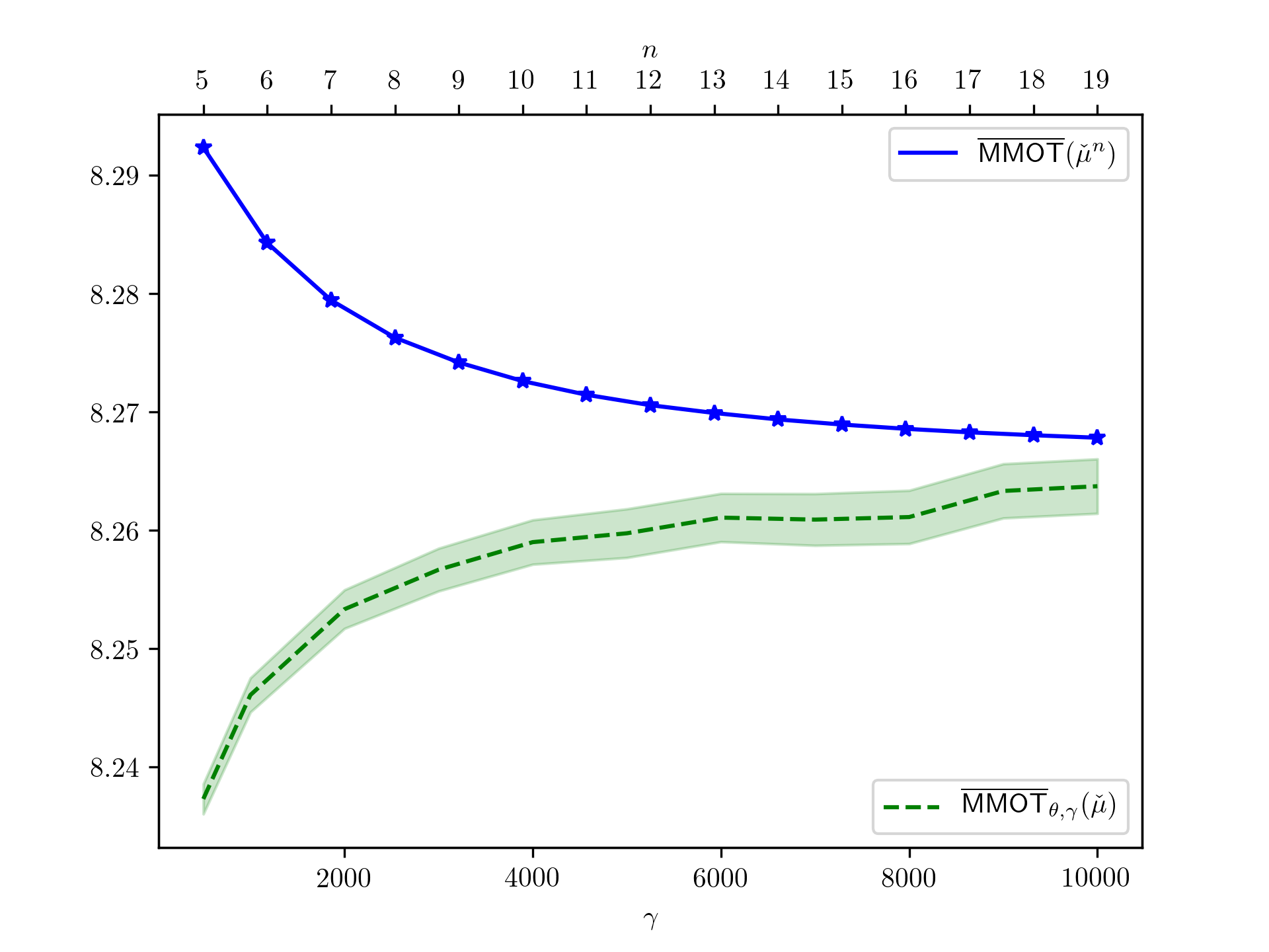
Figure 1: Numerical convergence analysis for the case of a spread option and $p=2$ from Table 2

The blue line shows how the numerical values obtained by the LP method depend on the discretisation parameter $n$, see Appendix A. The green line shows the analogue for the NN method, and the penalization parameter $\gamma$. Since the numerical method in the NN case is based on stochastic gradient descent, the final values can vary. The green error bands indicate the standard deviation of the obtained numerical values across 10 different sample runs. The higher the penalization parameter $\gamma$ is chosen, the more the final values vary.

Table 3: Improvement of bounds with information from additional maturities

	$\overline{\mathsf{OT}}$	$\overline{\mathsf{MMOT}}$		$\underline{\mathsf{OT}}$	$\underline{\mathsf{MMOT}}$
$T$	1	2	4	1	2	4
Spread Option ($p=2$)	8.337	8.254	7.920	0.335	0.416	0.776
Basket Option ($K=0$)	$1.500$	1.500	1.501	0.025	0.260	0.345

Numerically optimal values for the example in Section 4.1 obtained by the NN implementation. The penalization uses $\beta_{\gamma}(x)=\gamma\cdot x_{+}^{2}$ where $\gamma$ is set to $2500$ times the number of time steps in the optimization problem.

Figure 2: Spread Option ($p=2$). Numerically optimal couplings at the final time point obtained using the NN approach.

Maximizer, $T=1$

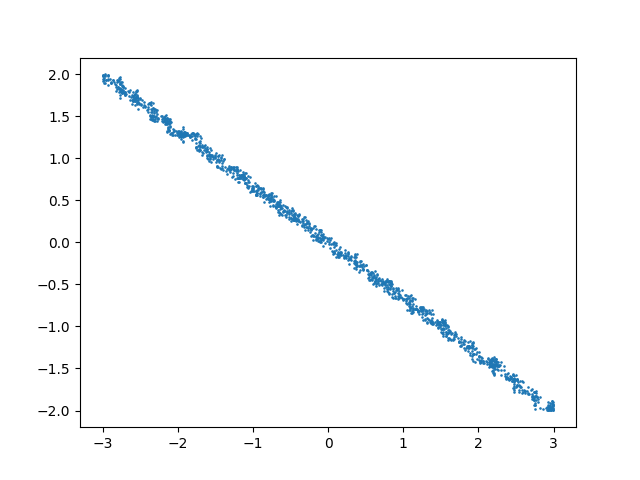
Maximizer, $T=2$

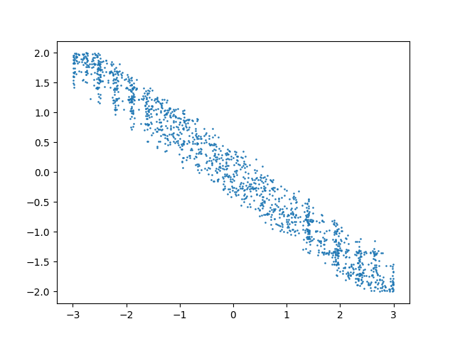
Maximizer, $T=4$

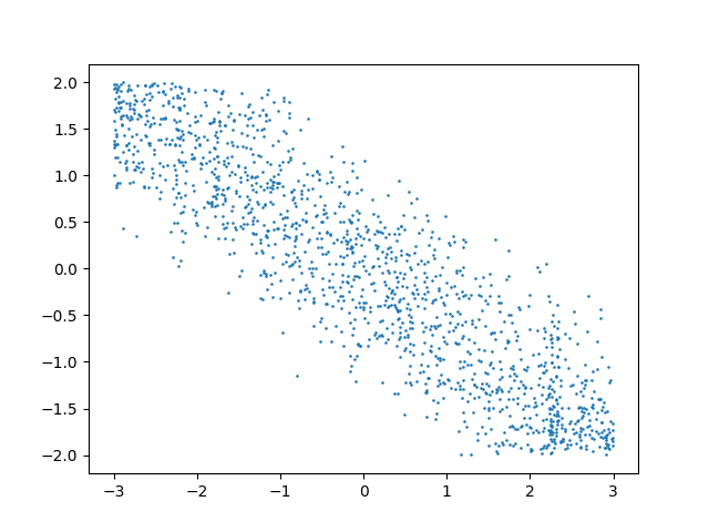
Minimizer, $T=1$

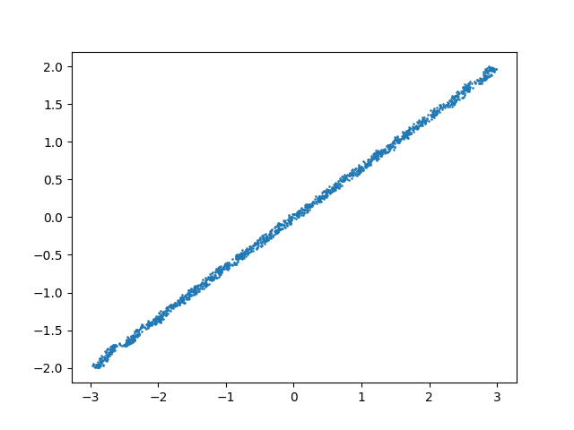
Minimizer, $T=2$

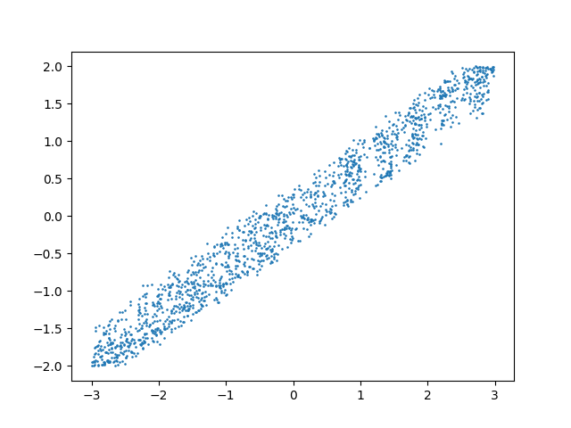
Minimizer, $T=4$

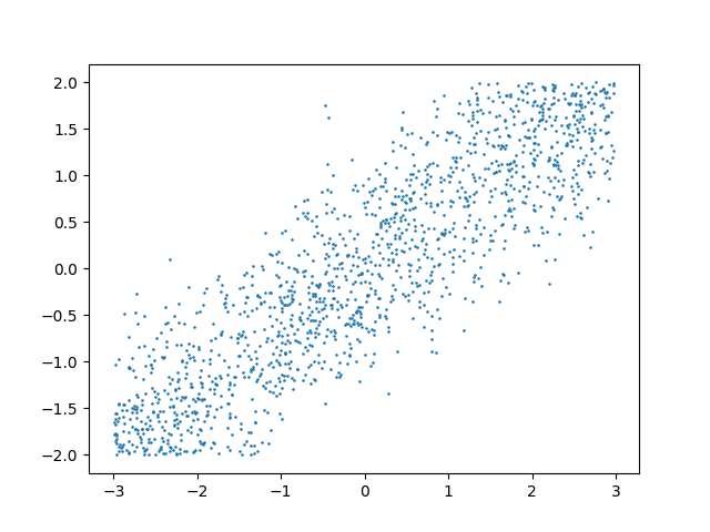
Figure 3: Basket Option ($K=0$). Numerically optimal couplings at final time point obtained using the NN approach.

Maximizer, $T=1$

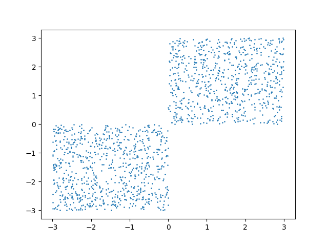
Maximizer, $T=2$

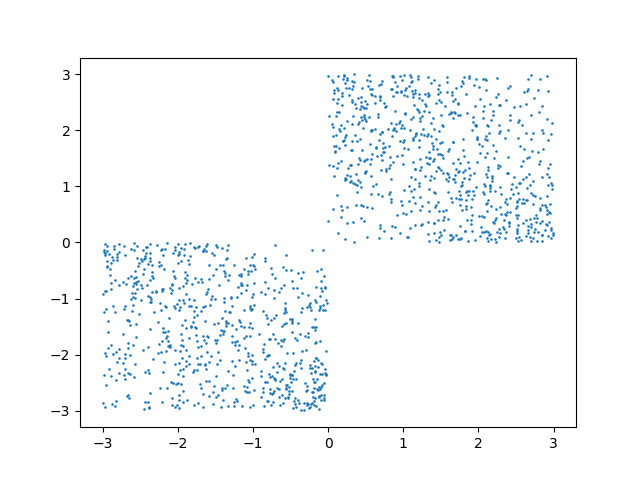
Maximizer, $T=4$

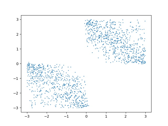
Minimizer, $T=1$

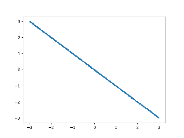
Minimizer, $T=2$

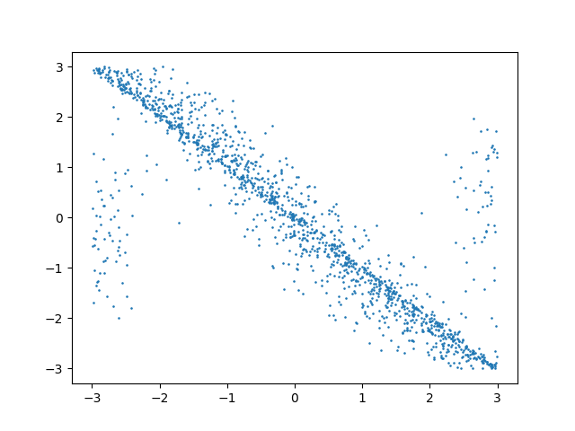
Minimizer, $T=4$

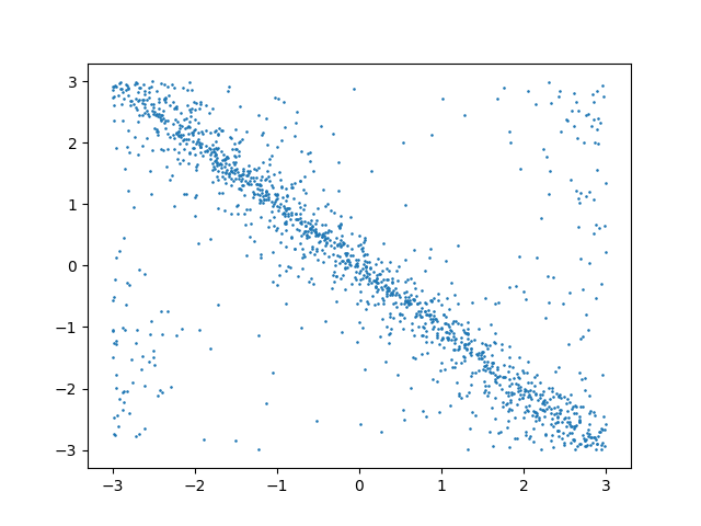
Figure 4: Numerically optimal couplings at the final time point using the LP approach for $T=2$.

Maximizer Spread ($p=2$)

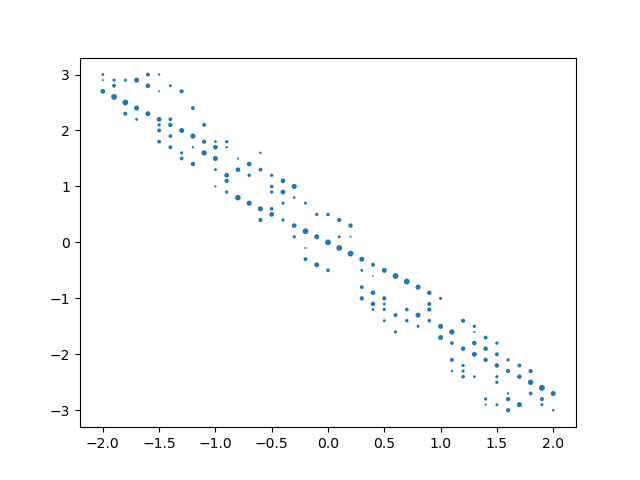
Minimizer Spread ($p=2$)

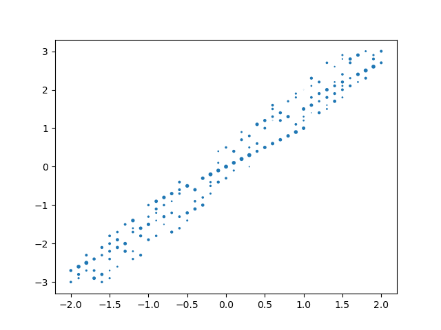
Maximizer Basket ($K=0$)

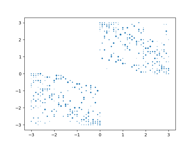
Minimizer Basket ($K=0$)

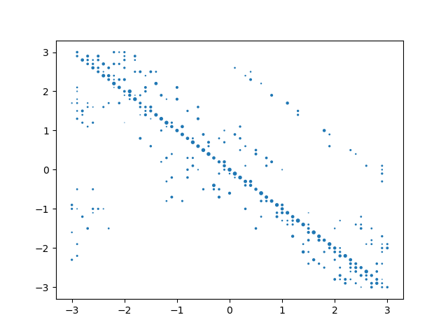
Having built confidence in the numerical precision of our methods, we now turn to examining how they capture and price the effect of using additional information. Recall that Table 1 summarises the marginal distribution information available in the context of the simple example studied in this section. Table 3 shows the difference in numerical bounds from working with marginal distributions at 1, 2, or 4 maturities. We see that for both the spread and the basket option, significantly narrower bounds are obtained with each additional piece of information. The absolute bounds are still quite wide even with four time steps of information used: $(0.78,7.92)$ for the spread and $(0.35,1.50)$ for the basket option. This suggests that applicability of the obtained bounds as a pricing tool will be case-dependent. However, in all cases, it is the relative comparison of how the bounds behave across assets and when additional information is added which is informative. It gives quantitative insight into dependence and structural implications of pricing information across assets and maturities. To narrow bounds further we would need to include modelling assumption or significantly constraining new information, cf. Henry-Labordère, (2013); Lütkebohmert and Sester, (2018). We note that in the case of the upper bound for the basket option the additional information did not change the bound indicating the additional information is not relevant for this upper no-arbitrage price. We believe it is a strength of the methodology we present here to be able to pick up also such cases. In this particular case, the reasons can be understood analytically. Indeed, let us focus on the case $K=0$ in Table 3 but similar comments apply to other strikes in Table 2, as well as to results presented in Table 4.2 in the next section. Using $(x+y)^{+}\leq x^{+}+y^{+}$ we have

$$\overline{\mathsf{MMOT}}(\check{\mu})=\sup_{\pi\in\mathcal{M}(\check{\mu})}\leavevmode\nobreak\ \int(x_{T,1}+x_{T,2})^{+}\,d\pi\leq\int x_{T,1}d\mu_{T,1}+\int x_{T,2}d\mu_{T,2}$$

and this upper bound is independent of $\pi$ and is attained by any $\pi\in\mathcal{M}(\check{\mu})$ for which $x_{T,1}$ and $x_{T,2}$ have the same sign $\pi$-a.s. This is a weak requirement and is typically attained by many couplings, as seen in Figure 3 below.

Figures 2 and 3 showcase the joint distribution between the first asset ($x$-axis) and the second asset ($y$-axis) at the final time point. These are obtained using the NN approach via (9). As expected, for the cases $T=2$ the depicted optimizers look very similar to the ones obtained by linear programming displayed in Figure 4. The most notable characteristic of the observed optimizers is that in most cases (again, except for the supremum problem of the basket option), the optimal couplings become smoother when more time steps are involved. This is an interesting feature: where the OT problem returns a deterministic (Monge) coupling, when we add the martingale constraint the Monge coupling is not feasible but the optimizers are still concentrated on lower dimensional sets, see Ghoussoub et al., (2019). When we add further time points it adds more constraints and the models become less and less singular, i.e., having a more diffused support.

4.2 Lognormal marginals

We turn now to distributions more representative of real market conditions. Specifically, instead of uniform marginals we consider lognormal ones. As before, we consider two assets and, in this case, three distinct maturities. The way the marginal distributions are set up is that both assets have the same distributions at time points $1$ and $3$, but at time $2$, the marginals vary. In particular, the marginal distributions imply that the first asset accumulates most of its volatility between time points $2$ and $3$, while the second asset accumulates most if its volatility between time points $1$ and $2$. More precisely, we set $\mu_{t,i}\sim\exp(\sigma_{t,i}X-\sigma_{t,i}^{2}/2)$, where $X$ follows a standard normal distribution and $\sigma_{1,1}=\sigma_{1,2}=0.1,\sigma_{3,1}=\sigma_{3,2}=0.2,\sigma_{2,1}=0.11,\sigma_{2,2}=0.19$.

We first calculate price bounds using only marginal information and trading between the first and third time points. Then, we include the intermediate maturity (the second time point) as well. This brings the additional marginal information which implies the asymmetry in the way the two assets accumulate their volatility as well as the ability to re-balance the hedging position at the intermediate time point. For the implementation, the neural network method remains unchanged compared to Section 4.1, just larger batch size is used to cope with the added difficulty of unbounded support of the marginals. For the LP method, we now use discretisation as described in (Alfonsi et al.,, 2019, Equation (6.5)).

Table 4: Improvement of bounds for the lognormal marginals

$\overline{\mathsf{MMOT}}$
$T=2$	$\overline{\mathsf{MMOT}}$
$T=3$	$\underline{\mathsf{MMOT}}$
$T=2$	$\underline{\mathsf{MMOT}}$
$T=3$
LP	NN	LP	NN	LP	NN	LP	NN
Spread Option ($p=2$)
0.1587	0.1625	0.1320	0.1359	0.0000	0.0010	0.0244	0.0269
Basket Option (at the money, $K=2$)
0.1593	0.1593	0.1585	0.1593	0.0192	0.0191	0.0397	0.0423

Numerically optimal values for Section 4.2 lognormal example obtained using the linear programming (LP) and neural network (NN) implementations. The case $T=2$ uses only the marginal information at the first and the last time point, while for the case $T=3$ the marginal distributions at an intermediate maturity are also given along with the ability to rebalance the hedging positions.

Table 4.2 reports the resulting values. We see that the bounds tighten significantly with the addition of the intermediate maturity information and hedging, highlighting the capacity of our methods to capture and quantify the benefit of such additional information for pricing problems. The only example is given by the upper bound for the basket option, which was expected as explained in Section 4.1. Despite the added difficulty of the non-compactly supported marginals, as compared to Section 4.1, the LP and NN methods still produce very similar values in all cases. Most importantly, the effect of the improved bounds by including the additional time point is clearly more significant than the differences between the numerical values, and hence the qualitative message one can derive from this example is robust with respect to the numerical method used.

4.3 A test of accuracy: comparison to theoretical values

In this section we consider a sanity check example where we can compare the numerical values to theoretical ones. Since generally, it is very difficult to obtain theoretical values for MMOT problems, we must refer to a structurally simple problem. To this end, consider uniform marginals: $\mu_{1,i}=\mathcal{U}([-1,1])$ and $\mu_{2,i}=\mathcal{U}([-2,2])$ for $i=1,...,d$, and a cost function $c(x):=\sum_{i=1}^{d}\sum_{j=1}^{d}c_{i,j}x_{2,i}x_{2,j}$ for some $c_{i,j}\geq 0$ chosen randomly in the interval $[0,1]$. Such costs are studied further in Section 5. An optimizer for this problem is characterized by the comonotone coupling among the dimensions at the final time step. The associated value can thus be computed to an arbitrary precision by sampling. Nevertheless, this analytical simplicity does not imply that the example is particularly easy to solve numerically. The singular nature of the optimizers is a feature which presents a challenge for numerical convergence.

Table 4.2 showcases the accuracy of the numerical methods in this example. Overall, especially for $d=2,3$, the relative errors are quite small, below $1\%$ relative error (in absolute terms, depending on the random cost functions, the true optimal values were typically around $3$ to $10$). For the LP method, higher error values are expected for increasing $d$, since fewer support points for the discretisation in each dimension can be used. The reason is that the total number of variables in the LP is limited due to working memory, and given by $\prod_{t=1}^{2}\prod_{i=1}^{d}n_{t,i}$ where $n_{t,i}$ is the number of support points of the discretised approximation of $\mu_{t,i}$. A priori, the NN method does not have this drawback. The error for the NN method is governed by the term $\int\beta_{\gamma}^{*}(\frac{d\pi}{d\theta})\,d\theta$, where $\pi$ is an optimal coupling and $\theta$ the measure chosen for penalization. In particular when any optimizer $\pi$ is highly singular with respect to $\theta$, as in this example, this error term can increase sharply with increasing dimension as well. While theoretically, this can be overcome by increasing $\gamma$, the error of the numerical method has to be taken into account as well, see also Figure 1.

Table 5: Relative error of the numerical methods

Dimension $d$	2	3	4
LP	0.04%	0.78%	3.12%
NN	0.08%	0.61%	2.05%

Average relative error over 100 sample runs with varying cost functions is showcased for Example 4.3.

4.4 Real-world application: foreign exchange data

We close the examples section with an example using FX data. We work with option data on three currency pairs, $X_{1}=\textrm{GBPUSD}$, $X_{2}=\textrm{EURUSD}$, $X_{3}=\textrm{EURGBP}$. The data was collected from a Bloomberg terminal on the 28 January 2019 for three tenors: 1y, 1.5y and 2 years out. We converted prices from FX specific convention to the strike convention used here and also converted put prices into call prices using the put-call parity, see Figure 5. Given the prevailing low interest rates and the illustrative nature of the example, we assumed all domestic and foreign interest rates are equal so no discounting was needed. We denote the prices of the three assets by $X_{t,i}$, where $t=0$ is the current exchange rate on 28/01/19 and $t=1,2,3$ corresponds to the three tenors above. To test our methodology, we study a synthetic spread process between two USD denominated exchange rates: $(X_{t,1}-\frac{X_{0,1}}{X_{0,2}}X_{t,2})_{t=1,2,3}$. In particular we calculate the range of arbitrage free prices for an Asian call option on this spread process over the time points $t=1,2,3$, i.e., we consider the payoff

(13) $$c(X)=\left(\frac{1}{3}\sum_{t=1}^{3}X_{t,1}-\frac{X_{0,1}}{X_{0,2}}X_{t,2}\right)^{+}.$$

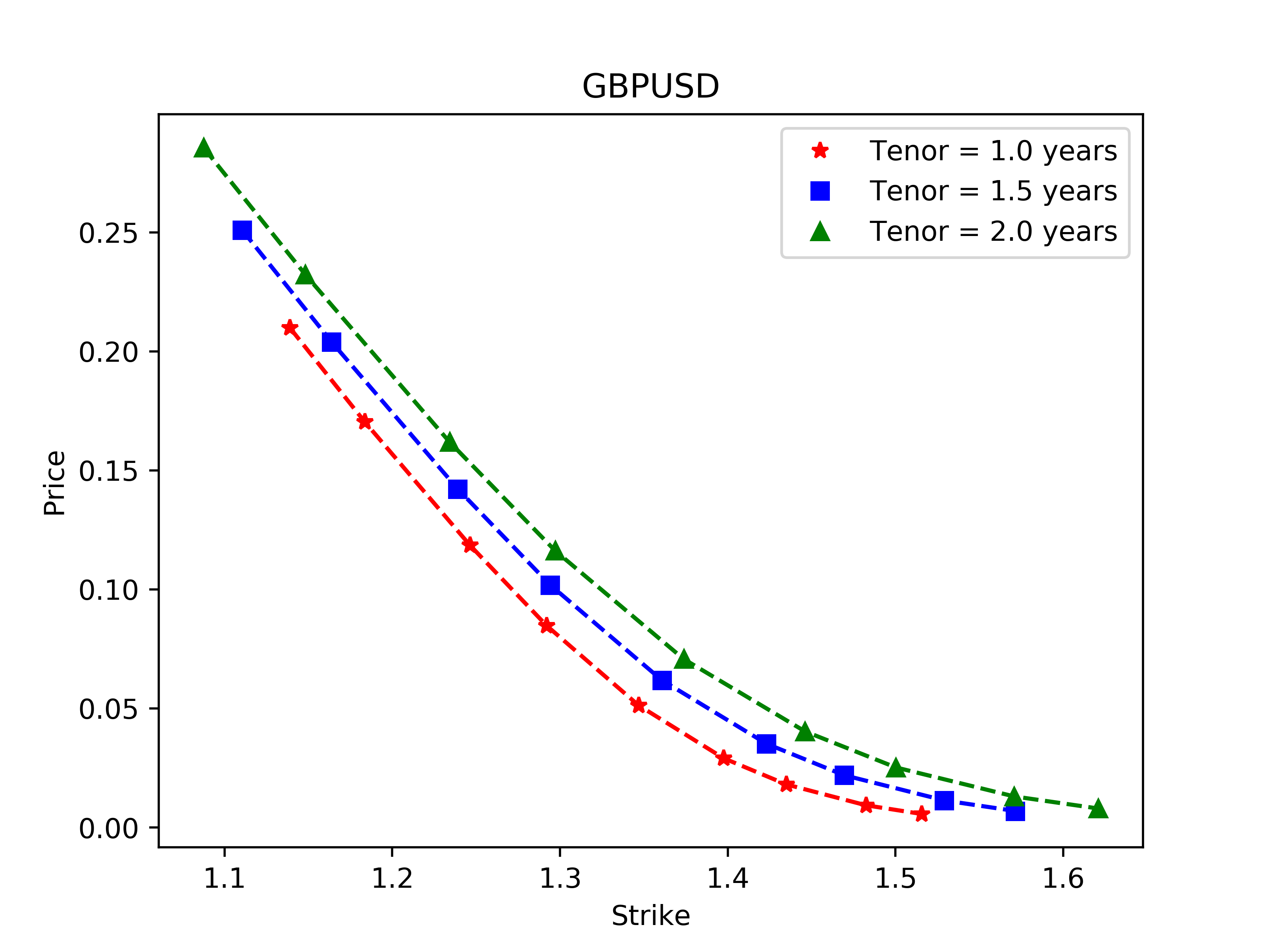
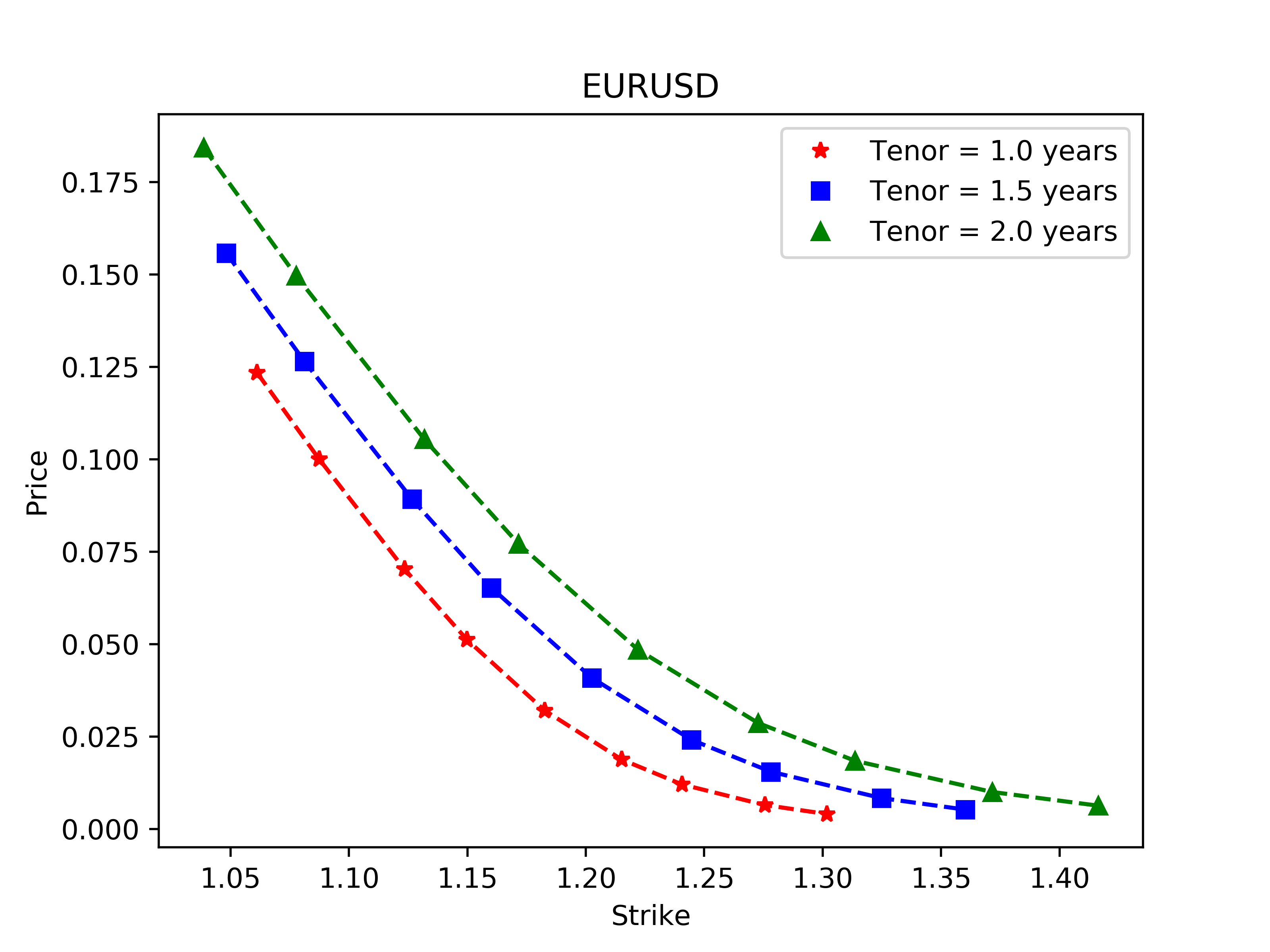
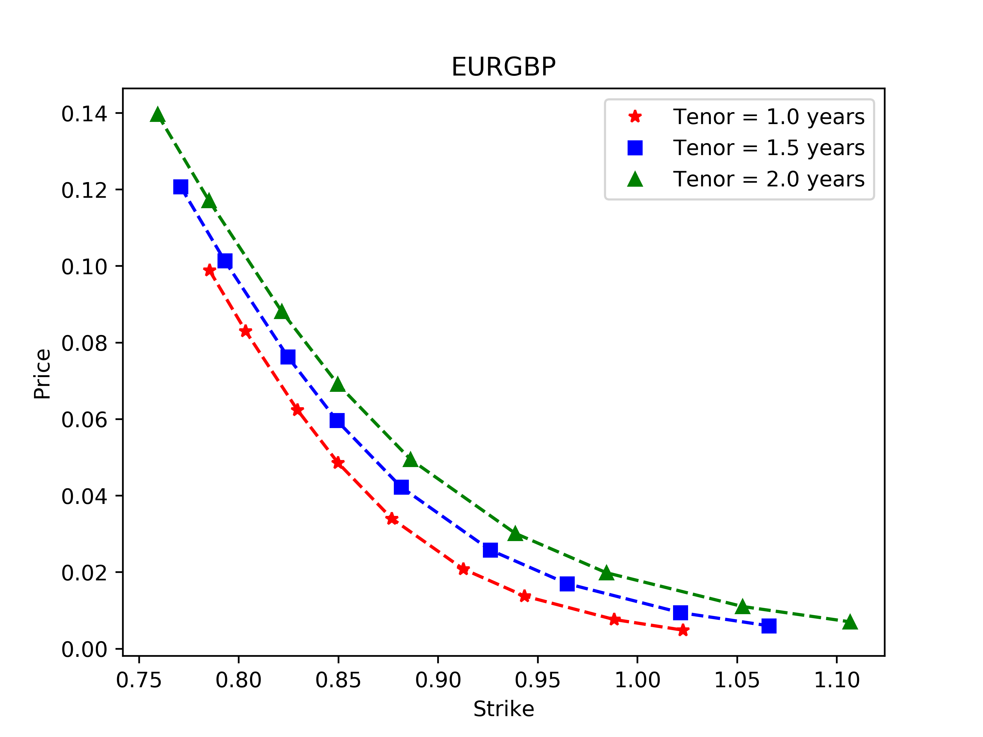
Figure 5: Foreign exchange option data on three different currency pairs. Date of retrieval for the prices is January 28, 2019.

The table showcases data for call option prices for three different currency pairs. Further, initial values at time point 0 are given by $\textrm{GBPUSD}=1.32$, $\textrm{EURUSD}=1.14$, $\textrm{EURGBP}=1.15$.

We employ the NN methodology to compute the optimal values. In practice, we modify slightly the formulation of $\overline{{\mathcal{D}}}^{m}$ in Section 3.2. Instead of estimating the risk-neutral marginal distributions from the call/put prices and considering all static position $\varphi_{t,i}\in\mathfrak{N}_{l,1,m}$, we directly consider $\varphi_{t,i}$ which are linear combinations of traded call options. Figure 6 displays the range of no-arbitrage prices under two different information structures: without and with the option prices for the third currency pair. We expect that the EURGBP prices, $X_{3}=X_{t,2}/X_{t,1}$, capture important information about the correlation structure between $X_{1}$ and $X_{2}$ which should be material for pricing of our Asian option even if $X_{3}$ is not explicitly present in its payoff. This is indeed true as seen from the price tightening in Figure 6 between the upper and the lower bars. In particular, we see that the upper bound shrinks by nearly 50% when the additional information is included. Furthermore, for both scenarios, we consider also the impact of the ability to hedge dynamically in the assets as compared to only taking static positions in the options. Again, this leads to a tightening of the bounds, albeit less pronounced. We believe that this example showcases the capacity of our methodology to capture, in a fully non-parametric but quantitative manner, the importance of market information for a given pricing problem. Naturally, its full potential should be explored on a much larger and more comprehensive range of market data/problems. This is left for future research.

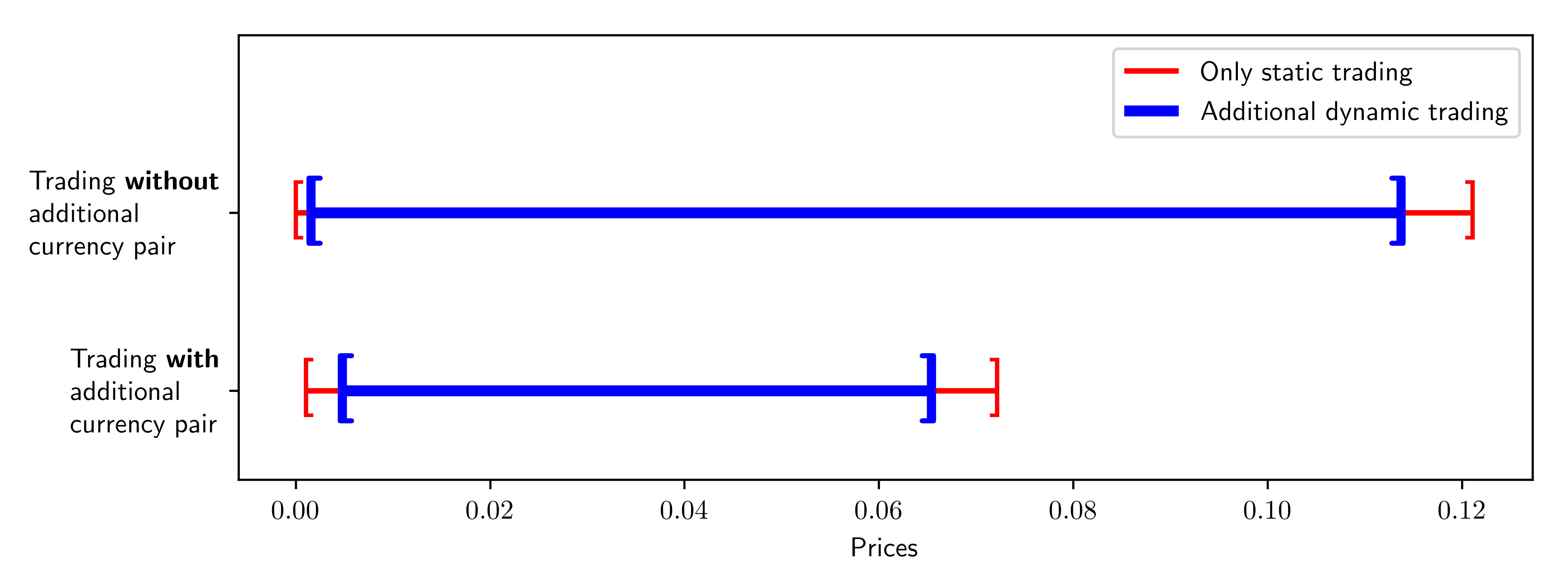
Figure 6: Price intervals for an Asian call option written on the spread process between $\rm{GBPUSD}$ and $\rm{EURUSD}$.

Numerically computed ranges of arbitrage free prices for the Asian option with payoff in (13). For the red lines, all models (without martingale assumption), or equivalently without dynamic trading are considered. For the blue lines, only martingale models are considered. For the bottom lines, additional trading in call options written on $X_{t,3}=X_{t,2}/X_{t,1}$ is allowed.

5 A structural result on the covariance functional

In this section we study a two-period model, i.e., $T=2$, and develop structural results for the optimizers. Our study was partly inspired by Figure 2 where the two time step optimizer has the structure of a probability distribution on a line superimposed with the OT optimizer. We shall see in Theorem 5.3 below that this structure is in fact universal, under certain assumptions on the marginal distributions. To make notation simpler, we write $X=(X_{i})_{1\leq i\leq d}$, $Y=(Y_{i})_{1\leq i\leq d}$ instead of $X_{1}=(X_{1,i})$, $X_{2}=(X_{2,i})$, and $\mu=(\mu_{i})$, $\nu=(\nu_{i})$ instead of $\check{\mu}_{1}=(\mu_{1,i})$, $\check{\mu}_{2}=(\mu_{2,i})$. Hence we consider the one-step martingales $(X_{i},Y_{i})_{1\leq i\leq d}$ with marginals $X_{i}\sim\mu_{i}$, $Y_{i}\sim\nu_{i}$. For each $\pi={\mathcal{L}}(X,Y)\in\mathcal{M}(\mu,\nu)$, define $\pi^{1}=\pi\circ X^{-1}$, $\pi^{2}=\pi\circ Y^{-1}$ to be the $d$-dimensional marginals of $\pi$. We assume that all $\mu_{i},\nu_{i}$ have finite second moments. Define $[d]=\{1,2,...,d\}$.

We will consider the maximization problem (1) with the cost functional which concerns the mutual covariance of the value of assets at the terminal time

(14) $$c(Y)=\sum_{1\leq i<j\leq d}c_{ij}Y_{i}Y_{j},\quad\text{where}\quad c_{ij}\geq 0.$$

We can assume without loss of generality that every $Y_{j}$ is involved in $c(Y)$, that is, for each $j\in[d]$ there exists nonzero $c_{ij}$ or $c_{jk}$; otherwise we may simply ignore the $j$-th asset in our optimization problem. We can regard $[d]$ as the set of nodes of a graph where $i,j$ is connected by an (undirected) edge if $c_{ij}>0$. Then $[d]$ is decomposed into connected subgraphs, and it is clear that the MMOT problem can be decomposed accordingly. Therefore, without loss of generality we can assume that $[d]$ is connected.

For our structural result, we also introduce the following notion.

Definition 5.1 (Linear Increment of Marginals (LIM)).

We say that marginals $(\mu_{i},\nu_{i})_{1\leq i\leq d}$ satisfy LIM if there exists a centered non-Dirac probability measure $\kappa$, and positive constants $a_{1},...,a_{d}$ such that ν_i = μ_i * a_i_# κ where ${a_{i}}_{\#}\kappa$ is the push-forward of $\kappa$ by the scaling map $x\mapsto a_{i}x$. In other words, ${\mathcal{L}}(Y_{i})={\mathcal{L}}(X_{i}+a_{i}Z)$ where $Z\sim\kappa$ is independent of $X$ and $\mathbb{E}[Z]=0$, $\mathbb{P}[Z\neq 0]>0$.

Example 5.2.

LIM holds when each pair of marginals $\mu_{i},\nu_{i}$ are Gaussians with the same mean and increasing variance.

Theorem 5.3.

Let $c(Y)=\sum_{1\leq i<j\leq d}c_{ij}Y_{i}Y_{j}$ and assume $c_{ij}$’s induce a connected graph on $[d]$. Suppose $(\mu_{i},\nu_{i})_{1\leq i\leq d}$ satisfy LIM with constant $a=(a_{1},...,a_{d})$. Let $L$ be the one-dimensional subspace of $\mathbb{R}^{d}$ spanned by $a$. Then every MMOT $\pi$ for the maximization problem (1), if disintegrated as $\pi(dx,dy)=\pi_{x}(dy)\pi^{1}(dx)$, satisfies:

1. ${\rm{supp}}\,\pi_{x}\subset L+x\quad\pi^{1}$ - almost every $x,$

2. $\pi^{1}$ is an optimal transport plan in $\Pi(\mu_{1},...,\mu_{d})$ for the maximization problem with the corresponding cost $c(X)=\sum_{1\leq i<j\leq d}c_{ij}X_{i}X_{j}$.

Moreover if $d=2$ or $3$ and the first marginals $(\mu_{i})_{i}$ are continuous (i.e., $\mu_{i}(\{x\})=0$ for all $x\in\mathbb{R}$ and $i\in[d]$), then $\pi^{1}$ is unique for every MMOT $\pi$.

To prove the theorem, we shall need the following lemma.

Lemma 5.4.

Let $c(x)=\sum_{1\leq i<j\leq d}c_{ij}x_{i}x_{j}$ and assume $c_{ij}$’s induce a connected graph on $[d]$. Let $\lambda_{ij}=\sqrt{c_{ij}\frac{a_{j}}{a_{i}}}$, $\sigma_{ij}=\sqrt{c_{ij}\frac{a_{i}}{a_{j}}}$, and $g_{ij}(x)=\frac{1}{2}\big{(}\lambda_{ij}x_{i}-\sigma_{ij}x_{j}\big{)}^{2}$ for each $i<j$. Define $G(x)=\sum_{i<j}g_{ij}(x)$, and let $H_{x_{0}}(x)=G(x_{0})+\nabla G(x_{0})\cdot(x-x_{0})$ be the affine tangent function of $G$ at $x_{0}\in\mathbb{R}^{d}$. Then {x ∈R^d  —  G(x)=H_x_0(x) } = x_0 + L, where $L$ is the one-dimensional subspace of $\mathbb{R}^{d}$ spanned by $a=(a_{1},...,a_{d})$.

Proof 5.5.

Note that $x\mapsto g_{ij}(x)$ is constant if $a_{j}x_{i}-a_{i}x_{j}$ is constant. Hence $G$ is constant on $x_{0}+L$. Since $G$ is smooth and convex, this implies that $\nabla G$ is constant on $x_{0}+L$, yielding $x_{0}+L\subset K:=\{x\in\mathbb{R}^{d}\,|\,G(x)=H_{x_{0}}(x)\}$.

Conversely, clearly $G$ is an affine function on $K$, and since $g_{ij}$ are convex, all $g_{ij}$ are also affine on $K$. But any nonzero $g_{ij}$ can be affine only when $a_{j}x_{i}-a_{i}x_{j}$ is constant. Since $x_{0}\in K$ and $[d]$ is connected, this implies that $K\subset x_{0}+L$.

Proof 5.6 (Proof of Theorem 5.3).

Let $x=(x_{1},...,x_{d})$, $y=(y_{1},...,y_{d})\in\mathbb{R}^{d}$. We will construct functions $\phi_{i}\in L^{1}(\mu_{i})$, $\psi_{j}\in L^{1}(\nu_{j})$, $h:\mathbb{R}^{d}\to\mathbb{R}^{d}$ such that

(15) $$\sum_{i=1}^{d}\phi_{i}(x_{i})+\sum_{i=1}^{d}\psi_{i}(y_{i})+h(x)\cdot(y-x)\geq c(y)\quad on\quad\mathbb{R}^{d}\times\mathbb{R}^{d},$$

but for any solution $\pi^{*}\in\mathcal{M}(\mu,\nu)$ to the problem (1), we have

(16) $$\sum_{i=1}^{d}\phi_{i}(x_{i})+\sum_{i=1}^{d}\psi_{i}(y_{i})+h(x)\cdot(y-x)=c(y)\quad\pi^{*}-a.e.\,(x,y).$$

We shall call the triplet $(\phi_{i},\psi_{i},h)$ a dual optimizer, and $\pi^{*}$ a multi-marginal martingale optimal transport (MMOT); see Lim, (2016). Along the proof, we will see that the equality (16) implies that $y-x\in L$.

To begin, let $f_{i}\in L^{1}(\mu_{i})$, $i=1,...,d$, be a dual optimizer for the optimal transport with the cost $c(x)$, that is, for any optimal transport $\gamma\in\Pi(\mu_{1},...,\mu_{d})$

(17) $$\sum_{i=1}^{d}f_{i}(x_{i})\geq c(x)\quad\forall x\in\mathbb{R}^{d},$$

(18) $$\sum_{i=1}^{d}f_{i}(x_{i})=c(x)\quad\gamma-a.e.\,x.$$

For the existence of such a dual optimizer, see Villani, (2003, 2009). Recall the functions $g_{ij}$ and $G$ in Lemma 5.4, and note that $G(x)=-c(x)+\sum_{i=1}^{d}b_{i}x_{i}^{2}$ for some $b_{i}\geq 0$. Define $\phi_{i}(x_{i})=f_{i}(x_{i})-b_{i}x_{i}^{2}$ and $\psi_{i}(y_{i})=b_{i}y_{i}^{2}$. Then the above may be rewritten as

(19) $$-\sum_{i=1}^{d}\phi_{i}(x_{i})\leq G(x)\quad\forall x\in\mathbb{R}^{d},$$

(20) $$-\sum_{i=1}^{d}\phi_{i}(x_{i})=G(x)\quad\gamma-a.e.\,x.$$

Next, define $h(x)=-\nabla G(x)$, so that we have

(21) $$G(x)-h(x)\cdot(y-x)\leq G(y),\text{ and the equality holds iff }y-x\in L$$

by Lemma 5.4. With (19) this implies (15). Moreover, notice that if $(x,y)$ satisfies the equality (16), then it holds $y-x\in L$ and the equality (18).

Now we will construct a multi-marginal martingale transport $\pi^{*}\in\mathcal{M}(\mu,\nu)$ such that $\pi^{*}$ is concentrated on the equality set in (16), that is $\pi^{*}(P)=1$ where

$$P:=\{(x,y)\in\mathbb{R}^{d}\times\mathbb{R}^{d}\,|\,\sum_{i=1}^{d}\phi_{i}(x_{i})+\sum_{i=1}^{d}\psi_{i}(y_{i})+h(x)\cdot(y-x)=c(y)\}.$$

We also define $P_{1}:=\{x\in\mathbb{R}^{d}\,|\,\sum_{i=1}^{d}f_{i}(x_{i})=c(x)\}$. In order to construct $\pi^{*}(dx,dy)=\pi^{*}_{x}(dy)\pi^{*1}(dx)$, firstly set $\pi^{*1}$ to be an optimal transport, i.e. $\pi^{*1}\in\Pi(\mu_{1},...,\mu_{d})$ and $\pi^{*1}(P_{1})=1$. Next, let $\sigma$ be the distribution of the vector $(a_{1}Z,\ldots,a_{d}Z)$ with $Z\sim\kappa$, and note that $\sigma(L)=1$ and $\sigma\in\Pi({a_{1}}_{\#}\kappa,...,{a_{d}}_{\#}\kappa)$.

For each $x\in\mathbb{R}^{d}$, define the kernel $\pi^{*}_{x}$ to be the $\sigma$ translated by $x$. As $\sigma$ has its barycenter at $0$, $\pi^{*}_{x}$ is clearly a martingale kernel. Now to ensure that $\pi^{*}\in\mathcal{M}(\mu,\nu)$, it remains to show that $\pi^{*2}\in\Pi(\nu_{1},...,\nu_{d})$. But notice that this follows from the facts $\pi^{*1}\in\Pi(\mu_{1},...,\mu_{d})$, $\sigma\in\Pi({a_{1}}_{\#}\kappa,...,{a_{d}}_{\#}\kappa)$, the definition of $\pi^{*}_{x}$, and finally the assumption LIM, i.e. $\nu_{i}=\mu_{i}*{a_{i}}_{\#}\kappa$.

Now observe that $\pi^{*}_{x}(L+x)=1$ and $\pi^{*1}(P_{1})=1$ imply, by (19), (20), and (21), that $\pi^{*}(P)=1$. This immediately implies the optimality of $\pi^{*}$ to the MMOT problem (1) by the following standard argument: let $\pi\in\mathcal{M}(\mu,\nu)$ be any multi-marginal martingale transport. By integrating both sides of (15) by $\pi$, we get ∑_i=1^d ∫ϕ_i  dμ_i + ∑_i=1^d ∫ψ_i  dν_i ≥∫c  dπ since $\int h(x)\cdot(y-x)\,\pi(dx,dy)=0$. On the other hand, as $\pi^{*}(P)=1$ we get ∑_i=1^d ∫ϕ_i  dμ_i + ∑_i=1^d ∫ψ_i  dν_i = ∫c  dπ^*. Hence $\int c\,d\pi^{*}\geq\int c\,d\pi$, and the optimality of $\pi^{*}$ follows. The argument also shows conversely that any solution $\pi^{*}$ must be concentrated on $P$, and this implies $\pi^{*}_{x}(L+x)=1$ and $\pi^{*1}(P_{1})=1$ by (19), (20), (21). But $\pi^{*1}(P_{1})=1$ precisely means that $\pi^{*1}$ is an optimal transport as claimed in the second part of the theorem.

Lastly, we prove the uniqueness statement. Let $\pi$ be an MMOT and let $\gamma=\pi\circ X^{-1}$. As we have just shown, $\gamma$ satisfies (17), (18) for some $f_{i}\in L^{1}(\mu_{i})$, $i=1,...,d$. If $d=2$, it is well known in optimal transport theory (see Villani, (2003)) that the contact set $P_{1}=\{x\in\mathbb{R}^{2}\ |\ \sum_{i=1}^{2}f_{i}(x_{i})=c(x)\}$ is a subset of a nondecreasing graph, that is

$$(x,y),(x^{\prime},y^{\prime})\in P_{1}\text{ and }x<x^{\prime}\implies y\leq y^{\prime},$$

and this property immediately implies that there exists a unique probability measure concentrated on $P_{1}$ which respects the marginal constraints $\mu_{1},\mu_{2}$. This proves the uniqueness assertion for $d=2$.

Now let $d=3$ and $P_{1}=\{x\in\mathbb{R}^{3}\ |\ \sum_{i=1}^{3}f_{i}(x_{i})=c(x)\}$. By permuting the indices $1,2,3$ if necessary, by connectedness there are two cases of cost function

$$c(x)=c_{12}x_{1}x_{2}+c_{13}x_{1}x_{3}+c_{23}x_{2}x_{3},\quad\text{or}\quad c(x)=c_{12}x_{1}x_{2}+c_{23}x_{2}x_{3},$$

where $c_{ij}>0$. Again consider (17), (18). By the standard technique, called Legendre-Fenchel transform, we can assume that $f_{i}$’s are convex functions, and hence in particular $f_{i}$ is differentiable $\mu_{i}$-a.s.. Let $A_{i}$ be the set of differentiable points of $f_{i}$, $i=1,2,3$. Now assume $(x_{1},x_{2},x_{3})\in P_{1}$ and $x_{1}\in A_{1}$. Then by the first-order condition, (17), (18) implies

$$f_{1}^{\prime}(x_{1})=c_{12}x_{2}+c_{13}x_{3},$$

where in the latter cost function case $c_{13}=0$. Let $Q_{1}(x_{1}):=\{(x_{2},x_{3})\in A_{2}\times A_{3}\ |\ f_{1}^{\prime}(x_{1})=c_{12}x_{2}+c_{13}x_{3}\}$, which is a linearly decreasing, or vertical, graph in $x_{2}x_{3}$-plane. On the other hand, the following ‘conditional contact set’

$$P_{1}(x_{1}):=\{(x_{2},x_{3})\in A_{2}\times A_{3}\ |\ \sum_{i=1}^{3}f_{i}(x_{i})=c(x)\}$$

is a nondecreasing graph as before. But notice that in fact $P_{1}(x_{1})$ is a graph of a nondecreasing function defined on $A_{2}$, since again (17), (18) implies

$$f_{2}^{\prime}(x_{2})=c_{12}x_{1}+c_{23}x_{3}.$$

We conclude that the intersection

$$P_{1}(x_{1})\cap Q_{1}(x_{1})$$

consists of at most one element for $\mu_{1}$-almost every $x_{1}$, and this implies that there exist two functions $x_{2}=\phi(x_{1}),x_{3}=\psi(x_{1})$, well-defined $\mu_{1}$-a.s., such that any probability measure concentrated on $P_{1}$ is in fact concentrated on the set

$$G:=\{(x_{1},x_{2},x_{3})\ |\ x_{2}=\phi(x_{1}),x_{3}=\psi(x_{1})\}.$$

By standard averaging argument, this implies the uniqueness of $\gamma$. This completes the proof of Theorem 5.3.

Appendix A Discretization

This section shows a sample discretization and formulation of an MMOT problem as an LP. We take the case $T=2$ for the spread option from Table 1. Recall that $\mu_{1,1}=\mu_{1,2}={\mathcal{U}}\big{(}[-1,1]\big{)}$, $\mu_{2,1}={\mathcal{U}}\big{(}[-3,3]\big{)}$ and $\mu_{2,2}={\mathcal{U}}\big{(}[-2,2]\big{)}$. Define discrete approximating probability measures via (6), i.e.,

(22) $$\begin{split}\alpha^{i}_{k}\quad=\quad\mu_{1,i}^{n}\big{(}\big{\{}k/n\big{\}}\big{)}&\quad:=\quad\int_{[(k-1)/n,(k+1)/n)}\big{(}1-|nk-x|\big{)}\mu_{1,i}(dx),\\ \beta^{i}_{k}\quad=\quad\mu_{2,i}^{n}\big{(}\big{\{}k/n\big{\}}\big{)}&\quad:=\quad\int_{[(k-1)/n,(k+1)/n)}\big{(}1-|nk-y|\big{)}\mu_{2,i}(dy),\end{split}$$

so that $\mu^{n}_{1,i}\preceq_{cx}\mu^{n}_{2,i}$ and ${\mathcal{W}}_{1}(\mu^{n}_{t,i},\mu_{t,i})\leq 1/n$ for $t,i=1,2$. Furthermore

$$\alpha^{1}_{-n}\leavevmode\nobreak\ =\leavevmode\nobreak\ \alpha^{1}_{n}\leavevmode\nobreak\ =\leavevmode\nobreak\ 1/4n\quad\mbox{and}\quad\alpha^{1}_{i}\leavevmode\nobreak\ =\leavevmode\nobreak\ 1/2n\mbox{ for }-n+1\leq i\leq n-1,$$

$$\alpha^{2}_{-n}\leavevmode\nobreak\ =\leavevmode\nobreak\ \alpha^{2}_{n}\leavevmode\nobreak\ =\leavevmode\nobreak\ 1/4n\quad\mbox{and}\quad\alpha^{2}_{j}\leavevmode\nobreak\ =\leavevmode\nobreak\ 1/2n\mbox{ for }-n+1\leq j\leq n-1,$$

$$\beta^{1}_{-3n}\leavevmode\nobreak\ =\leavevmode\nobreak\ \beta^{1}_{3n}\leavevmode\nobreak\ =\leavevmode\nobreak\ 1/12n\quad\mbox{and}\quad\beta^{1}_{k}\leavevmode\nobreak\ =\leavevmode\nobreak\ 1/6n\mbox{ for }-3n+1\leq k\leq 3n-1,$$

$$\beta^{2}_{-2n}\leavevmode\nobreak\ =\leavevmode\nobreak\ \beta^{2}_{2n}\leavevmode\nobreak\ =\leavevmode\nobreak\ 1/8n\quad\mbox{and}\quad\beta^{2}_{l}\leavevmode\nobreak\ =\leavevmode\nobreak\ 1/4n\mbox{ for }-2n+1\leq l\leq 2n-1.$$

Then $\overline{\mathsf{P}}_{2/n}(\check{\mu}_{1}^{n},\check{\mu}_{2}^{n})$ in the mentioned case of the spread option as objective is given by the following linear program (LP):

$$\max_{(p_{i,j,k,l})\in\mathbb{R}_{+}^{M}}\leavevmode\nobreak\ \sum_{i=-n}^{n}\sum_{j=-n}^{n}\sum_{k=-3n}^{3n}\sum_{l=-2n}^{2n}p_{i,j,k,l}|y^{1}_{k}-y^{2}_{l}|^{p}$$

s.t. $$\sum_{j=-n}^{n}\sum_{k=-3n}^{3n}\sum_{l=-2n}^{2n}p_{i,j,k,l}\leavevmode\nobreak\ =\leavevmode\nobreak\ \alpha^{1}_{i},\quad\mbox{for }i=-n,\ldots,n,$$

$$\sum_{i=-n}^{n}\sum_{k=-3n}^{3n}\sum_{l=-2n}^{2n}p_{i,j,k,l}\leavevmode\nobreak\ =\leavevmode\nobreak\ \alpha^{2}_{j},\quad\mbox{for }j=-n,\ldots,n,$$

$$\sum_{i=-n}^{n}\sum_{j=-n}^{n}\sum_{l=-2n}^{2n}p_{i,j,k,l}\leavevmode\nobreak\ =\leavevmode\nobreak\ \beta^{1}_{k},\quad\mbox{for }k=-3n,\ldots,3n,$$

$$\sum_{i=-n}^{n}\sum_{j=-n}^{n}\sum_{k=-3n}^{3n}p_{i,j,k,l}\leavevmode\nobreak\ =\leavevmode\nobreak\ \beta^{2}_{l},\quad\mbox{for }l=-2n,\ldots,2n,$$

$$\left|\sum_{k=-3n}^{3n}\sum_{l=-2n}^{2n}\big{(}y^{1}_{k}-x^{1}_{i}\big{)}p_{i,j,k,l}\right|\leavevmode\nobreak\ \leq\leavevmode\nobreak\ 2/n\sum_{k=-3n}^{3n}\sum_{l=-2n}^{2n}p_{i,j,k,l},$$

$$\hskip 227.62204pt\quad\mbox{for }i,j=-n,\ldots,n,$$

$$\left|\sum_{k=-3n}^{3n}\sum_{l=-2n}^{2n}\big{(}y^{2}_{l}-x^{2}_{j}\big{)}p_{i,j,k,l}\right|\leavevmode\nobreak\ \leq\leavevmode\nobreak\ 2/n\sum_{k=-3n}^{3n}\sum_{l=-2n}^{2n}p_{i,j,k,l},$$

$$\hskip 227.62204pt\quad\mbox{for }i,j=-n,\ldots,n,$$

where

$$x^{1}_{i}\leavevmode\nobreak\ =\leavevmode\nobreak\ i/n,\quad\mbox{for }i=-n,\ldots,n,$$

$$x^{2}_{j}\leavevmode\nobreak\ =\leavevmode\nobreak\ j/n,\quad\mbox{for }j=-n,\ldots,n,$$

$$y^{1}_{k}\leavevmode\nobreak\ =\leavevmode\nobreak\ k/n,\quad\mbox{for }k=-3n,\ldots,3n,$$

$$y^{2}_{l}\leavevmode\nobreak\ =\leavevmode\nobreak\ l/n,\quad\mbox{for }l=-2n,\ldots,2n,$$

and $M:=(2n+1)^{2}(6n+1)(4n+1)$, $N:=(6n+1)(4n+1)$.

References

- Alfonsi et al., (2019) Alfonsi, A., Corbetta, J., and Jourdain, B. (2019). Sampling of probability measures in the convex order and and computation of robust option price bounds. Int. J. Theo. App. Finance, 22(03):1950002.
- Backhoff-Veraguas and Pammer, (2019) Backhoff-Veraguas, H. and Pammer, G. (2019). Stability of martingale optimal transport and weak optimal transport. arXiv:1904.04171.
- Baker, (2012) Baker, D. (2012). Martingales with specified marginal. PhD thesis, Université Pierre et Marie-Curie - Paris VI.
- Bartl et al., (2017) Bartl, D., Cheridito, P., Kupper, M., and Tangpi, L. (2017). Duality for increasing convex functionals with countably many marginal constraints. Banach J. Math. Analysis, 11(1):72–89.
- (5) Beiglböck, M., Cox, A., and Huesmann, M. (2017a). Optimal Transport and Skorokhod Embedding. Invent. Math., 208(2):327–400.
- Beiglböck et al., (2013) Beiglböck, M., Henry-Labordére, P., and Penkner, F. (2013). Model-independent bounds for option prices–a mass transport approach. Financ. Stoch., 17(3):477–501.
- (7) Beiglböck, M., Nutz, M., and Touzi, N. (2017b). Complete duality for martingale optimal transport on the line. Ann. Probab., 45(5):3038–3074.
- Benamou et al., (2015) Benamou, J.-D., Carlier, G., Cuturi, M., Nenna, L., and Peyré, G. (2015). Iterative bregman projections for regularized transportation problems. SIAM Journal on Scientific Computing, 37(2):A1111–A1138.
- Breeden and Litzenberger, (1978) Breeden, D. T. and Litzenberger, R. H. (1978). Prices of state-contingent claims implicit in option prices. J. Business, 51(4):621–651.
- Brown et al., (2001) Brown, H., Hobson, D., and Rogers, C. (2001). Robust hedging of barrier options. Math. Finance, 11(3):285–314.
- Burzoni et al., (2019) Burzoni, M., Frittelli, M., Hou, Z., Maggis, M., and Obłój, J. (2019). Pointwise arbitrage pricing theory in discrete time. Math. Oper. Res., 43(3):1034–1057.
- Chacon, (1977) Chacon, R. V. (1977). Potential processes. Trans. Amer. Math. Soc., 226:39–58.
- Cox and Obłój, (2011) Cox, A. and Obłój, J. (2011). Robust pricing and hedging of double no-touch options. Finance Stoch., 15(3):573–605.
- Cuturi, (2013) Cuturi, M. (2013). Sinkhorn distances: Lightspeed computation of optimal transport. In Advances in neural information processing systems, pages 2292–2300.
- De March, (2018) De March, H. (2018). Entropic approximation for multi-dimensional martingale optimal transport. arXiv:1812.11104.
- Dolinsky and Soner, (2014) Dolinsky, Y. and Soner, H. (2014). Martingale optimal transport and robust hedging in continuous time. Probab. Theory Relat. Fields, 160(1-2):391–427.
- Eckstein and Kupper, (2019) Eckstein, S. and Kupper, M. (2019). Computation of optimal transport and related hedging problems via penalization and neural networks. Appl. Math. Opt. (online) DOI: 10.1007/s00245-019-09558-1.
- Fournier and Guillin, (2015) Fournier, N. and Guillin, A. (2015). On the rate of convergence in wasserstein distance of the empirical measure. Probab. Theory Relat. Fields, 162(3-4):707–738.
- Galichon et al., (2014) Galichon, A., Henry-Labordére, P., and Touzi, N. (2014). A stochastic control approach to no-arbitrage bounds given marginals, with an application to lookback options. Ann. Appl. Probab., 24(1):312–336.
- Ghoussoub et al., (2019) Ghoussoub, N., Kim, Y.-H., and Lim, T. (2019). Structure of optimal martingale transport plans in general dimensions. Ann. Probab., 47(1):109–164.
- Gulrajani et al., (2017) Gulrajani, I., Ahmed, F., Arjovsky, M., Dumoulin, V., and Courville, A. C. (2017). Improved training of wasserstein gans. In Advances in neural information processing systems, pages 5767–5777.
- Guo and Obłój, (2019) Guo, G. and Obłój, J. (2019). Computational methods for martingale optimal transport problems. Ann. Appl. Probab., 29(9):3311–3347.
- Henry-Labordère, (2013) Henry-Labordère, P. (2013). Automated option pricing: Numerical methods. Int. J. Theo. App. Finance, 16(8):1350042.
- Hobson, (1998) Hobson, D. (1998). Robust hedging of the lookback option. Finance Stoch., 2(4):329–347.
- Hou and Obłój, (2018) Hou, Z. and Obłój, J. (2018). Robust pricing-hedging dualities in continuous time. Finance Stoch., 22:511–567.
- Knight, (1921) Knight, F. (1921). Risk, Uncertainty and Profit. Boston: Houghton Mifflin.
- Kramkov and Xu, (2019) Kramkov, D. and Xu, Y. (2019). An optimal transport problem with backward martingale constraints motivated by insider trading. arXiv:1906.03309.
- Lim, (2016) Lim, T. (2016). Multi-martingale optimal transport. arXiv:1611.01496.
- Lütkebohmert and Sester, (2018) Lütkebohmert, E. and Sester, J. (2018). Tightening robust price bounds for exotic derivatives. Available at SSRN 3290503.
- Obłój, (2004) Obłój, J. (2004). The Skorokhod embedding problem and its offspring. Probability Surveys, 1:321–392.
- Seguy et al., (2018) Seguy, V., Damodaran, B. B., Flamary, R., Courty, N., Rolet, A., and Blondel, M. (2018). Large-scale optimal transport and mapping estimation. In ICLR 2018-International Conference on Learning Representations, pages 1–15.
- Strassen, (1965) Strassen, V. (1965). The existence of probability measures with given marginals. Ann. Math. Stat., 36(2):423–439.
- Villani, (2003) Villani, C. (2003). Topics in optimal transportation, volume 58 of Graduate Studies in Mathematics. American Mathematical Society, Providence, RI.
- Villani, (2009) Villani, C. (2009). Optimal Transport. Old and New, volume 338 of Grundlehren der mathematischen Wissenschaften. Springer.
- Wang et al., (2013) Wang, R., Peng, L., and Yang, J. (2013). Bounds for the sum of dependent risks and worst value-at-risk with monotone marginal densities. Finance Stoch., 17(2):395–417.
- Wiesel, (2019) Wiesel, J. (2019). Continuity of the martingale optimal transport problem on the real line. arXiv:1905.04574.
- Zaev, (2015) Zaev, D. A. (2015). On the monge-kantorovich problem with additional linear constraints. Math. Notes, 98(5):725–741.