The sigma function over a family of cyclic trigonal curves with a singular fiber

Abstract.

In this paper we investigate the behavior of the sigma function over the family of cyclic trigonal curves $X_{s}$ defined by the equation $y^{3}=x(x-s)(x-b_{1})(x-b_{2})$ in the affine $(x,y)$ plane, for $s\in D_{\varepsilon}:=\{s\in{\mathbb{C}}||s|<\varepsilon\}$. We compare the sigma function over the punctured disc $D_{\varepsilon}^{*}:=D_{\varepsilon}\setminus\{0\}$ with the extension over $s=0$ that specializes to the sigma function of the normalization $X_{\widehat{0}}$ of the singular curve $X_{s=0}$ by investigating explicitly the behavior of a basis of the first algebraic de Rham cohomology group and its period integrals. We demonstrate, using modular properties, that sigma, unlike the theta function, has a limit. In particular, we obtain the limit of the theta characteristics and an explicit description of the theta divisor translated by the Riemann constant.

2010 MSC: Primary: 32G20, 14H45. Secondary: 14H42, 14H40, 14H10.

1. Introduction

The study of the Jacobi variety or the theta function over families of curves with singular members has a long history and is still very active. Classically, Clebsh and Gordan introduced generalized theta functions for specific degenerations of hyperelliptic curves [9, §81]. Kodaira classified the singular fibers of elliptic surfaces [19]. Igusa showed that there exists a (generalized) Jacobian fibration over a family of curves with a finite number of degenerate members which have at most nodal singularities [17].

However, in our work we focus on the analytic limit of a specific section of (a translate of) the theta line bundle, which turned out to be an important tool in integrable dynamics and number theory (modular aspects of Riemann period matrices). Our goal is to look at a family of Jacobians, which we call a Jacobian fibration for simplicity even though our general fiber has dimension three, while the central fiber has dimension two (therefore the definition of fibration does not apply) over a family of curves with a central fiber that has a nodal singularity, and extend (a translate of) the theta line bundle over the Jacobian of the normalized central fiber; for this, we use a section, known as sigma function.

Based on classical constructions by Weierstrass and Klein, and further study by Baker [35, 18, 3, 2], Weierstrass’ (elliptic) sigma function was generalized to non-singular curves in Weierstrass canonical form; notably, unlike the theta function, sigma obeys an addition rule that can be expressed in terms of meromorphic functions on the curve [8, 12, 15, 22, 31]; moreover, Buchstaber and Leykin investigated the behavior of the sigma functions in moduli, under the heat equation and the Gauss-Manin connection [7, 14]. Using these results, in [5, 4] the sigma function is analyzed over a degenerating family of hyperelliptic curves.

In this paper, we investigate the behavior of the sigma function of a degenerating family of trigonal curves $X_{s}$, given by affine equation $y^{3}=x(x-s)(x-b_{1})(x-b_{2})$ for $s$ in the unit disc

$$D_{\varepsilon}=\{s\in{\mathbb{C}}\ |\ |s|<\varepsilon\}.$$

Our strategy is the following: in [10, 27], we obtained explicit properties of the sigma function ${\sigma_{X_{s}}}$ for the non-singular curve $X_{s}$ over the punctured disc $s\in D_{\varepsilon}^{*}=D_{\varepsilon}\setminus\{0\}$; in [25, 22], we analyzed ${\sigma_{X_{{\widehat{0}}}}}$ for the normalized curve $X_{\widehat{0}}$ of $X_{0}=X_{s=0}$ given by $y^{3}=x^{2}(x-b_{1})(x-b_{2})$. Now we consider the degenerating family of curves

$$\mathfrak{X}:=\{(x,y,s)\ |\ (x,y)\in X_{s},s\in D_{\varepsilon}\},$$

we will exhibit the first algebraic de Rham cohomology groups, whose generators are given by first and second-kind differentials, as well as their period matrices, for $X_{s}$ when $s\in D_{\varepsilon}^{*}$, and for $X_{\widehat{0}}$. We show the precise behavior of the integrals in Appendices A and B. Finally, in Section 4 we compare these objects over the non-singular fiber $X_{s}$ to those of $X_{\widehat{0}}$ at $s=0$. Using this analysis, we construct the sigma functions ${\sigma_{X_{s}}}$ and ${\sigma_{X_{{\widehat{0}}}}}$ of $X_{s}$ $(s\in D_{s}^{*})$ and of $X_{\widehat{0}}$. The relationship of the sigma function with the algebraic functions of the curve, particularly with the al function, which we had also previously constructed for the trigonal cyclic case [27] turns out to be essential.

Using the fact that a section of the divisor that gives the principal polarization with the given modular behavior over the family is unique, we view the sigma functions ${\sigma_{X_{s}}}$ and ${\sigma_{X_{{\widehat{0}}}}}$ as the canonical bases of the (translate) theta line bundles $\mathcal{L}_{\mathcal{J}_{s}}$ and $\mathcal{L}_{\mathcal{J}_{\widehat{0}}}$ on the Jacobi varieties, $\mathcal{J}_{s}$ and $\mathcal{J}_{\widehat{0}}$. Thus we obtain an explicit extension in the limit $s\longrightarrow 0$ from $\mathcal{L}_{\mathcal{J}_{s}}$, $s\in D_{\varepsilon}^{*}$, to $\mathcal{L}_{\mathcal{J}_{\widehat{0}}}$, and produce an explicit line bundle over the Jacobian fibration of the family. In the family, using the sigma functions, we provide the connection to the Jacobian of the desingularization $X_{\widehat{0}}$ over the central fiber instead of a generalized Jacobian considered by Igusa [17]. Recent progress on the study of the modular structure of the sigma functions by Eilbeck, Gibbons, Ônishi and Yasuda [14], based on the investigation of Buchstaber and Leykin [7], enables us to find the behavior of the sigma function as the period lattice varies. Using their results, we explicitly compare the structure of the limit of $\mathcal{L}_{\mathcal{J}_{s}}$ with that of $\mathcal{L}_{\mathcal{J}_{\widehat{0}}}$ and the ramified covering $\widetilde{D_{\varepsilon}^{*}}$ of $D_{\varepsilon}^{*}$ given by the cyclic group of order three. The definition of sigma involves theta characteristics; while the parity behavior of theta characteristics over families is well-known [1, 28], we need to compute explicitly the limit of the Riemann constant, which for our curves is translated by a multiple of the divisor at infinity on the affine part of the curve; in particular, we observe the behavior of the Weierstrass semigroup going from symmetric to non-symmetric under degeneration.

Since this degeneration can be regarded as a higher-genus version of the elliptic case, type IV in Kodaira’s classification, we apply the technique of this paper to the case of such degenerate family of elliptic curves in Appendix C. We make use of a very simple expression for the elliptic al function, whereas for the present trigonal case defining al requires an elaborate configuration of triple covers of the Jacobian. We give an explicit description of the behavior of sigma for the degeneration of type IV, which had not previously appeared as far as we know.

The contents of the paper are as follows. Section 2 gives a review of the sigma function ${\sigma_{X_{s}}}$ of $X_{s}$ for $s\in D_{\varepsilon}^{*}$. In Section 3, at $s=0$, by considering the normalization $X_{\widehat{0}}$ of the singular curve $X_{0}$ and the Jacobian $\mathcal{J}_{\widehat{0}}$, we give properties of the sigma function ${\sigma_{X_{{\widehat{0}}}}}$. In Section 4, we investigate the degeneration explicitly and present our main theorem. Appendix A due to Kazuhiro Aomoto is devoted to the study of the integrals associated with the period matrices over the degeneration. Using the results in Appendix A, Appendix B gives the explicit behavior of the period matrices in the limit $s\to 0$, the crux of this paper. Appendix C gives the behavior of the Weierstrass sigma function over the degenerating family of elliptic curves which is classified as type IV by Kodaira [19].

Shorthand. Throughout the paper, the symbol $d_{\geq n}(t)$ ($d_{>n}(t)$, respectively) denotes a formal power series of order $\geq n$ ($>n$, resp.) in the variable $t$ (single or multi-variable).

Acknowledgment The third named author thanks Tadashi Ashikaga for helpful and crucial comments, which led the Appendix C. Further he is also grateful to Chris Eilbeck, Victor Enolskii and Yoshihiro Ônishi for critical discussions and comments, and Takeo Ohsawa and Hajime Kaji for valuable comments. The third named author thanks the participants in Numadu-Shizuoka Kenkyukai and, specially, its organizer Yoshinori Machida. The second and third named authors were supported by the Grant-in-Aid for Scientific Research (C) of Japan Society for the Promotion of Science, Grant No. 18K04830 and Grant No. 16K05187 respectively. The first and the third named authors thank Victor Enolskii, Julia Bernatska, and Tony Shaska for their hospitality of the conference at Kiev August, 2018. The authors thank the anonymous reviewer for his/her helpful comments.

2. The sigma function of $y^{3}=x(x-s)(x-b_{1})(x-b_{2})$, $(s\neq 0)$

In this section, we review the properties of the sigma function of a non-singular cyclic trigonal curve of genus three following the papers [10, 26, 27].

2.1. Basic properties of $X_{s}$

We consider the non-singular cyclic trigonal curve $X_{s}$ of genus three, $g=3$, given by

$$X_{s}:=\Bigr{\{}(x,y)\ \Bigr{|}\ \begin{array}[]{rl}y^{3}=x(x-s)(x-b_{1})(x-b_{2})=:f(x)\end{array}\Bigr{\}}\cup\infty,$$

and its affine ring,

$$R_{s}:={\mathbb{C}}[x,y]/\left(y^{3}-x(x-s)(x-b_{1})(x-b_{2})\right).$$

Here we assume that $b_{0}:=0$, $b_{1}$, $b_{2}$ and $b_{3}:=s$ are mutually distinct complex numbers, in particular $s\neq 0$. The curve is given by a ramified cover of ${\mathbb{P}}$,

$$\pi_{1}(P)=x,\quad\pi_{2}(P)=y.$$

The finite branch points of $\pi_{1}$ are denoted by

(2.1) $$B_{0}:=(0,0),\quad B_{1}:=(b_{1},0),\quad B_{2}:=(b_{2},0),\quad B_{3}:=B_{s}=(s,0).$$

The curve $X_{s}$ has an automorphism $\widehat{\zeta}_{3}:X_{s}\to X_{s}$ given by $\widehat{\zeta}_{3}(x,y)=(x,\zeta_{3}y)$ for $\zeta_{3}:=$ $\mathrm{e}^{2\pi{\sqrt{-1}}/3}$.

The point $\infty$ in $X_{s}$ is a Weierstrass point. The natural weight of $R_{s}$ is assigned as $\mathrm{wt}_{\infty}(x)=-3$, $\mathrm{wt}_{\infty}(y)=-4$, since using the local parameter $t$ at $\infty$, we have

$$x=\frac{1}{t^{3}}(1+d_{\geq 1}(t)),\quad y=\frac{1}{t^{4}}(1+d_{\geq 1}(t)).$$

The Weierstrass non-gap sequence at $\infty$ is given by the following table.

Table 1: Weierstrass non-gap sequence of $X_{s}$
$-\mathrm{wt}_{\infty}$ 0 1 2 3 4 5 6 7 8 9 10 $\cdots$ ${\phi_{X_{s}}}$ 1 - - $x$ $y$ - $x^{2}$ $xy$ $y^{2}$ $x^{3}$ $x^{2}y$ $\cdots$

We denote the corresponding basis of monic monomials by $\phi_{X_{s}}$, i.e., ${\phi_{X_{s}0}}=1$, ${\phi_{X_{s}1}}=x$, ${\phi_{X_{s}2}}=y$, ${\phi_{X_{s}3}}=x^{2}$, $\cdots$. As a ${\mathbb{C}}$-vector space, we have the decomposition of $R_{s}$,

$$R_{s}=\bigoplus_{i=0}{\mathbb{C}}{\phi_{X_{s}i}}.$$

Corresponding to the non-gap sequence, we have the numerical semigroup $H_{s}:=\{3a+4b\}_{a,b\in{\mathbb{Z}}_{\geq 0}}$ $:=\langle 3,4\rangle$, where ${\mathbb{Z}}_{\geq 0}$ is the set of non-negative integers, i.e.,

$$H_{s}=\{0,3,4,6,7,\cdots\},\quad L_{s}={\mathbb{Z}}_{\geq 0}\setminus H_{s}=\{1,2,5\}.$$

The numerical semigroup $H_{s}$ is related to the Young diagram

$$\Lambda_{(3,1,1)}=\yng(3,1,1)$$

because $(1,2,5)-(0,1,2)=(1,1,3)$.

2.2. Differentials and Abelian integrals of $X_{s}$

The holomorphic one-forms or the differentials of the first kind on $X_{s}$ are given by

$${\nu^{I}_{X_{s}}}:=\begin{pmatrix}{\nu^{I}_{X_{s}1}}\\ {\nu^{I}_{X_{s}2}}\\ {\nu^{I}_{X_{s}3}}\end{pmatrix}:={}^{t}\left(\frac{dx}{3y^{2}},\frac{xdx}{3y^{2}},\frac{dx}{3y}\right)={}^{t}\left(\frac{{\phi_{X_{s}0}}dx}{3y^{2}},\frac{{\phi_{X_{s}1}}dx}{3y^{2}},\frac{{\phi_{X_{s}2}}dx}{3y^{2}}\right).$$

The divisor of ${\nu^{I}}$, $\mathrm{Div}({\nu^{I}}_{i})$, is linearly equivalent to $(2g-2)\infty=4\infty$. The differentials of the second kind (holomorphic except at $\infty$) are

$${\nu^{II}_{X_{s}}}:=\begin{pmatrix}{\nu^{II}_{X_{s}1}}\\ {\nu^{II}_{X_{s}2}}\\ {\nu^{II}_{X_{s}3}}\end{pmatrix},\quad{\nu^{II}_{X_{s}1}}:=-\frac{(5x^{2}-3\lambda_{3}x+\lambda_{2})dx}{3y},\quad$$

$${\nu^{II}_{X_{s}2}}:=-\frac{2xdx}{3y},\quad,{\nu^{II}_{X_{s}3}}:=-\frac{x^{2}dx}{3y^{2}},$$

where $\lambda_{3}=-s-b_{1}-b_{2}$ and $\lambda_{2}=s(b_{1}+b_{2})+b_{1}b_{2}$. The set of ${\nu^{I}_{X_{s}}}$ and ${\nu^{II}_{X_{s}}}$ gives a basis of the first algebraic de Rham cohomology of $X_{s}$.

The automorphism $\widehat{\zeta}_{3}$ of $X_{s}$ also acts on the one-forms,

$$\widehat{\zeta}_{3}({\nu^{I}_{X_{s}1}})=\zeta_{3}{\nu^{I}_{X_{s}1}},\quad\widehat{\zeta}_{3}({\nu^{I}_{X_{s}2}})=\zeta_{3}{\nu^{I}_{X_{s}2}},\quad\widehat{\zeta}_{3}({\nu^{I}_{X_{s}3}})=\zeta_{3}^{2}{\nu^{I}_{X_{s}3}},$$

$$\widehat{\zeta}_{3}({\nu^{II}_{X_{s}1}})=\zeta_{3}^{2}{\nu^{II}_{X_{s}1}},\quad\widehat{\zeta}_{3}({\nu^{II}_{X_{s}2}})=\zeta_{3}^{2}{\nu^{II}_{X_{s}2}},\quad\widehat{\zeta}_{3}({\nu^{II}_{X_{s}3}})=\zeta_{3}{\nu^{II}_{X_{s}3}}.$$

To define the Abelian integrals, we first consider the Abelian covering ${\widetilde{X}}_{s}$ of $X_{s}$, namely the abelianization of the quotient space of path space $\mathrm{Path}(X_{s})$ divided by homotopy equivalence with respect to the fixed point $\infty$. There are a natural projection $\kappa_{X}:{\widetilde{X}}_{s}\to X_{s}$ ($\kappa(\gamma_{P,\infty})=P$ for a path $\gamma_{P,\infty}\in{\widetilde{X}}_{s}$ from $\infty$ to $P\in X_{s}$) and a natural embedding $\iota_{X}:X_{s}\to{\widetilde{X}}_{s}$. The Abelian integral of the cyclic trigonal curve is defined as

$${\widetilde{w}_{X_{s}}}:{\widetilde{X}}_{s}\to{\mathbb{C}}^{3},\quad\left({\widetilde{w}_{X_{s}}}(P):=\int_{\gamma_{P,\infty}}{\nu^{I}_{X_{s}}}\right),$$

$${\widetilde{w}_{X_{s}}}:{\mathcal{S}}^{k}({\widetilde{X}}_{s})\to{\mathbb{C}}^{3},\quad{\widetilde{w}_{X_{s}}}(\gamma_{\infty,P_{1}},\gamma_{\infty,P_{2}},\ldots,\gamma_{\infty,P_{k}}):=\sum_{i=1}^{k}{\widetilde{w}_{X_{s}}}(\gamma_{\infty,P_{i}}),$$

where ${\mathcal{S}}^{k}{\widetilde{X}}_{s}$ is the $k$-th symmetric product of ${\widetilde{X}}_{s}$. The Abel-Jacobi theorem says that ${\widetilde{w}_{X_{s}}}:{\mathcal{S}}^{3}{\widetilde{X}}_{s}\to{\mathbb{C}}^{3}$ is a birational correspondence.

For the point $P_{i}$ near $\infty$ with a local parameter $t_{i}$ $(i=1,2,3)$, the variable $u_{j}=$ $\displaystyle{\sum_{i=1}^{3}\int_{\gamma_{P_{i},\infty}}{\nu^{I}_{X_{s}j}}}$ $(j=1,2,3)$ has the expansion,

(2.2) $$\begin{split}u_{1}&=\frac{1}{5}(t_{1}^{5}+t_{2}^{5}+t_{3}^{5})(1+d_{\geq 1}(t_{1},t_{2},t_{3})),\quad u_{2}=\frac{1}{2}(t_{1}^{2}+t_{2}^{2}+t_{3}^{2})(1+d_{\geq 1}(t_{1},t_{2},t_{3})),\\ u_{3}&=(t_{1}+t_{2}+t_{3})(1+d_{\geq 1}(t_{1},t_{2},t_{3})).\end{split}$$

The weight on the ring $R_{s}$ induces the weight of the components of the vectors $u$ in ${\mathbb{C}}^{3}$,

(2.3) $$\mathrm{wt}_{\infty}(u_{1})=5,\quad\mathrm{wt}_{\infty}(u_{2})=2\quad\mathrm{wt}_{\infty}(u_{3})=1.$$

2.3. Periods of $X_{s}$

The standard homology basis $(\alpha_{1},\alpha_{2},\alpha_{3},\beta_{1},\beta_{2},\beta_{3})$ satisfying the relations

$$\langle\alpha_{i},\beta_{j}\rangle=\delta_{ij},\quad\langle\alpha_{i},\alpha_{j}\rangle=0,\quad\langle\beta_{i},\beta_{j}\rangle=0\quad$$

is illustrated in Figure 1.

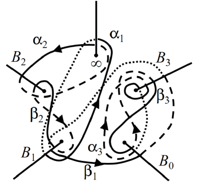
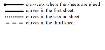
Figure 1. The basis of $H_{1}(X_{s},{\mathbb{Z}})$.

The complete Abelian integrals $\omega^{{\prime}}_{X_{s}}$ and ${\omega^{{\prime\prime}}_{X_{s}}}$ of the first kind are

$$\omega^{{\prime}}_{X_{s}ij}:=\frac{1}{2}\left(\int_{\alpha_{j}}{\nu^{I}_{X_{s}i}}\right),\quad{\omega^{{\prime\prime}}_{X_{s}ij}}:=\frac{1}{2}\left(\int_{\beta_{j}}{\nu^{I}_{X_{s}i}}\right),$$

and the complete Abelian integrals ${\eta^{{\prime}}_{X_{s}}}$ and ${\eta^{{\prime\prime}}_{X_{s}}}$ of the second kind are

$${\eta^{{\prime}}_{X_{s}ij}}:=\frac{1}{2}\left(\int_{\alpha_{j}}{\nu^{II}_{X_{s}i}}\right),\quad{\eta^{{\prime\prime}}_{X_{s}ij}}:=\frac{1}{2}\left(\int_{\beta_{j}}{\nu^{II}_{X_{s}i}}\right).$$

Since we have the integral along the contour $\gamma_{a}$ from $\infty$ to the branch point $B_{a}=(b_{a},0)$ $(a=0,1,2,3)$ [27], i.e.,

$$\omega_{X_{s}a}:=\int_{\infty}^{B_{a}}{\nu^{I}_{X_{s}}}=\int_{\gamma_{a}}{\nu^{I}_{X_{s}}},$$

the period matrices $\omega^{{\prime}}_{X_{s}}=(\omega^{{\prime}}_{X_{s}1},\omega^{{\prime}}_{X_{s}2},\omega^{{\prime}}_{X_{s}3})$ and ${\omega^{{\prime\prime}}_{X_{s}}}=({\omega^{{\prime\prime}}_{X_{s}1}},{\omega^{{\prime\prime}}_{X_{s}2}},{\omega^{{\prime\prime}}_{X_{s}3}})$ are described in terms of $\omega_{X_{s}a}$ as follows.

Lemma 2.1.

$${}^{t}(\omega^{{\prime}}_{X_{s}1},\omega^{{\prime}}_{X_{s}2},\omega^{{\prime}}_{X_{s}3},{\omega^{{\prime\prime}}_{X_{s}1}},{\omega^{{\prime\prime}}_{X_{s}2}},{\omega^{{\prime\prime}}_{X_{s}3}})={}^{t}((\omega_{X_{s}0},\omega_{X_{s}1},\omega_{X_{s}2},\omega_{X_{s}3})W_{X_{s}}),$$

where $W_{X_{s}}$ is a rank three matrix given by

$$\begin{split}W_{X_{s}}&:=\frac{1}{2}\begin{pmatrix}0&0&\widehat{\zeta}_{3}-\widehat{\zeta}_{3}^{2}&1-\widehat{\zeta}_{3}^{2}&0&1-\widehat{\zeta}_{3}^{2}\\ \widehat{\zeta}_{3}-1&0&0&\widehat{\zeta}_{3}-1&\widehat{\zeta}_{3}^{2}-1&0\\ 0&1-\widehat{\zeta}_{3}^{2}&0&0&1-\widehat{\zeta}_{3}^{2}&0\\ 0&0&\widehat{\zeta}_{3}^{2}-\widehat{\zeta}_{3}&\widehat{\zeta}_{3}^{2}-\widehat{\zeta}_{3}&0&\widehat{\zeta}_{3}^{2}-1\\ \end{pmatrix}\\ &=\frac{1-\widehat{\zeta}_{3}^{2}}{2}\begin{pmatrix}0&0&-\widehat{\zeta}_{3}^{2}&1&0&1\\ \widehat{\zeta}_{3}&0&0&\widehat{\zeta}_{3}&-1&0\\ 0&1&0&0&1&0\\ 0&0&\widehat{\zeta}_{3}^{2}&\widehat{\zeta}_{3}^{2}&0&-1\end{pmatrix}\\ \end{split}$$

The transpose is introduced because the action of $\widehat{\zeta}_{3}$ on the integrals is left-to-right. Noting that the integral over a path which is homotopic to a point, e.g.,

(2.4) $$(1-\widehat{\zeta}_{3}^{2})\omega_{X_{s}2}+\widehat{\zeta}_{3}^{2}(1-\widehat{\zeta}_{3}^{2})\omega_{X_{s}1}+\widehat{\zeta}_{3}(1-\widehat{\zeta}_{3}^{2})\omega_{X_{s}0}+(1-\widehat{\zeta}_{3}^{2})\omega_{X_{s}3}=0,$$

is equal to zero, $\omega_{X_{s}a}$ $(a=0,1,2,3)$ are described in terms of $\omega^{{\prime}}_{X_{s}}=(\omega^{{\prime}}_{X_{s}1},\omega^{{\prime}}_{X_{s}2},\omega^{{\prime}}_{X_{s}3})$:

Lemma 2.2.

$${}^{t}(\omega_{X_{s}0},\omega_{X_{s}1},\omega_{X_{s}2},\omega_{X_{s}3})={}^{t}((\omega^{{\prime}}_{X_{s}1},\omega^{{\prime}}_{X_{s}2},\omega^{{\prime}}_{X_{s}3})V_{X_{s}}),$$

where

$$V_{X_{s}}:=\frac{2}{3}\begin{pmatrix}\widehat{\zeta}_{3}^{2}-1&\widehat{\zeta}_{3}^{2}-1&0&\widehat{\zeta}_{3}^{2}-1\\ \widehat{\zeta}_{3}-\widehat{\zeta}_{3}^{2}&0&1-\widehat{\zeta}_{3}&\widehat{\zeta}_{3}-\widehat{\zeta}_{3}^{2}\\ \widehat{\zeta}_{3}^{2}-1&0&0&\widehat{\zeta}_{3}-1\\ \end{pmatrix}=\frac{2(\widehat{\zeta}_{3}^{2}-1)}{3}\begin{pmatrix}1&1&0&1\\ \widehat{\zeta}_{3}^{2}&0&\widehat{\zeta}_{3}&\widehat{\zeta}_{3}^{2}\\ 1&0&0&1\\ \end{pmatrix}.$$

Proof.

By considering the relation

$${}^{t}(\omega^{{\prime}}_{X_{s}1},\omega^{{\prime}}_{X_{s}2},\omega^{{\prime}}_{X_{s}3},0)={}^{t}((\omega_{X_{s}0},\omega_{X_{s}1},\omega_{X_{s}2},\omega_{X_{s}3})V)$$

with (2.4) and the matrix,

$$V=\frac{1-\widehat{\zeta}_{3}^{2}}{2}\begin{pmatrix}0&0&-\widehat{\zeta}_{3}^{2}&\widehat{\zeta}_{3}\\ \widehat{\zeta}_{3}&0&0&\widehat{\zeta}_{3}^{2}\\ 0&1&0&1\\ 0&0&\widehat{\zeta}_{3}^{2}&1\end{pmatrix},$$

the inverse matrix of $V$ is reduced to $V_{X_{s}}$ when (2.4) holds. ∎

Lemma 2.2 can be regarded as a generalization of Lemma C.2 which holds for the genus one case.

Corresponding to (C.2) and (C.3) in the genus one case, we have the following lemma:

Lemma 2.3.

$$\begin{pmatrix}{\omega^{{\prime\prime}}_{X_{s}11}}&{\omega^{{\prime\prime}}_{X_{s}12}}&{\omega^{{\prime\prime}}_{X_{s}13}}\\ {\omega^{{\prime\prime}}_{X_{s}21}}&{\omega^{{\prime\prime}}_{X_{s}22}}&{\omega^{{\prime\prime}}_{X_{s}23}}\\ {\omega^{{\prime\prime}}_{X_{s}31}}&{\omega^{{\prime\prime}}_{X_{s}32}}&{\omega^{{\prime\prime}}_{X_{s}33}}\\ \end{pmatrix}=\begin{pmatrix}-\zeta_{3}^{2}\omega^{{\prime}}_{X_{s}12}&-\zeta_{3}^{2}\omega^{{\prime}}_{X_{s}11}+\omega^{{\prime}}_{X_{s}12}&-\zeta_{3}\omega^{{\prime}}_{X_{s}13}\\ -\zeta_{3}^{2}\omega^{{\prime}}_{X_{s}22}&-\zeta_{3}^{2}\omega^{{\prime}}_{X_{s}21}+\omega^{{\prime}}_{X_{s}22}&-\zeta_{3}\omega^{{\prime}}_{X_{s}23}\\ -\zeta_{3}\omega^{{\prime}}_{X_{s}32}&-\zeta_{3}\omega^{{\prime}}_{X_{s}31}+\omega^{{\prime}}_{X_{s}32}&-\zeta_{3}^{2}\omega^{{\prime}}_{X_{s}33}\\ \end{pmatrix},$$

$$\begin{pmatrix}{\eta^{{\prime\prime}}_{X_{s}11}}&{\eta^{{\prime\prime}}_{X_{s}12}}&{\eta^{{\prime\prime}}_{X_{s}13}}\\ {\eta^{{\prime\prime}}_{X_{s}21}}&{\eta^{{\prime\prime}}_{X_{s}22}}&{\eta^{{\prime\prime}}_{X_{s}23}}\\ {\eta^{{\prime\prime}}_{X_{s}31}}&{\eta^{{\prime\prime}}_{X_{s}32}}&{\eta^{{\prime\prime}}_{X_{s}33}}\\ \end{pmatrix}=\begin{pmatrix}-\zeta_{3}{\eta^{{\prime}}_{X_{s}12}}&-\zeta_{3}{\eta^{{\prime}}_{X_{s}11}}+{\eta^{{\prime}}_{X_{s}12}}&-\zeta_{3}^{2}{\eta^{{\prime}}_{X_{s}13}}\\ -\zeta_{3}{\eta^{{\prime}}_{X_{s}22}}&-\zeta_{3}{\eta^{{\prime}}_{X_{s}21}}+{\eta^{{\prime}}_{X_{s}22}}&-\zeta_{3}^{2}{\eta^{{\prime}}_{X_{s}23}}\\ -\zeta_{3}^{2}{\eta^{{\prime}}_{X_{s}32}}&-\zeta_{3}^{2}{\eta^{{\prime}}_{X_{s}31}}+{\eta^{{\prime}}_{X_{s}32}}&-\zeta_{3}{\eta^{{\prime}}_{X_{s}33}}\\ \end{pmatrix}.$$

Proof.

Lemmas 2.1 and 2.2 directly give ${}^{t}({\omega^{{\prime\prime}}_{X_{s}1}},{\omega^{{\prime\prime}}_{X_{s}2}},{\omega^{{\prime\prime}}_{X_{s}3}})={}^{t}((\omega^{{\prime}}_{X_{s}1},\omega^{{\prime}}_{X_{s}2},$ $\omega^{{\prime}}_{X_{s}3})U_{X_{s}})$ and ${}^{t}({\eta^{{\prime\prime}}_{X_{s}1}},{\eta^{{\prime\prime}}_{X_{s}2}},{\eta^{{\prime\prime}}_{X_{s}3}})={}^{t}(({\eta^{{\prime}}_{X_{s}1}},{\eta^{{\prime}}_{X_{s}2}},{\eta^{{\prime}}_{X_{s}3}})U_{X_{s}})$ where

$$U_{X_{s}}:=\frac{2}{3}\begin{pmatrix}0&-\widehat{\zeta}_{3}^{2}&0\\ -\widehat{\zeta}_{3}^{2}&1&0\\ 0&0&-\widehat{\zeta}_{3}\end{pmatrix}.$$

∎

2.4. Jacobian and Abel-Jacobi map of $X_{s}$

The lattice $\Gamma_{s}$ in ${\mathbb{C}}^{3}$ is defined as

$$\Gamma_{s}:=\langle 2\omega^{{\prime}}_{X_{s}},2{\omega^{{\prime\prime}}_{X_{s}}}\rangle_{{\mathbb{Z}}}=\left\{2\omega^{{\prime}}_{X_{s}}\begin{pmatrix}a_{1}\\ a_{2}\\ a_{3}\end{pmatrix}+2{\omega^{{\prime\prime}}_{X_{s}}}\begin{pmatrix}a_{4}\\ a_{5}\\ a_{6}\end{pmatrix}\ \Bigr{|}\ a_{i}\in{\mathbb{Z}}\right\}\subset{\mathbb{C}}^{3},$$

and the Jacobi variety $\mathcal{J}_{X_{s}}$ is given by the canonical projection,

$$\kappa_{\mathcal{J}}:{\mathbb{C}}^{3}\to\mathcal{J}_{X_{s}}={\mathbb{C}}^{3}/\Gamma_{s}.$$

Using the Abelian integral ${\widetilde{w}_{X_{s}}}{}$, we define the Abel-Jacobi map ${w}_{X_{s}}{}$,

$${w}_{X_{s}}{}:{\mathcal{S}}^{k}X_{s}\to\mathcal{J}_{X_{s}}\quad{w}_{X_{s}}{}(P):=\kappa_{\mathcal{J}}\circ{\widetilde{w}_{X_{s}}}{}\circ\iota_{X}(P).$$

When $k=3$, ${w}_{X_{s}}{}$ is birational due to the Abel-Jacobi theorem. The normalized versions of these objects are given by

$${\nu^{I\circ}_{X_{s}}}:=\omega^{{\prime}-1}_{X_{s}}{\nu^{I}_{X_{s}}},\quad{\widetilde{w}}_{X_{s}}^{\circ}:=\omega^{{\prime}-1}_{X_{s}}{\widetilde{w}_{X_{s}}}{},\quad w_{X_{s}}^{\circ}:=\omega^{{\prime}-1}_{X_{s}}{w}_{X_{s}}{},$$

for the normalized period $(I_{3},\tau_{X_{s}}:=\omega^{{\prime}-1}_{X_{s}}{\omega^{{\prime\prime}}_{X_{s}}})$ and the normalized Jacobian,

$$\kappa_{\mathcal{J}}^{\circ}:{\mathbb{C}}^{3}\to\mathcal{J}_{X_{s}}^{\circ}:={\mathbb{C}}^{3}/\Gamma_{s}^{\circ},$$

where $I_{3}$ is the unit matrix and $\Gamma_{s}^{\circ}:=\langle I_{3},\tau_{X_{s}}\rangle_{\mathbb{Z}}$.

Lemma 2.4.

$$\tau_{X_{s}}=\begin{pmatrix}0&0&0\\ 0&1&0\\ 0&0&0\end{pmatrix}+\frac{\zeta_{3}}{|\omega^{{\prime}}_{X_{s}}|}T_{1}+\frac{\zeta_{3}^{2}}{|\omega^{{\prime}}_{X_{s}}|}T_{2},$$

where

$$T_{1}:=\left(\begin{matrix}(\omega^{{\prime}}_{X_{s}13}\omega^{{\prime}}_{X_{s}22}-\omega^{{\prime}}_{X_{s}12}\omega^{{\prime}}_{X_{s}23})\omega^{{\prime}}_{X_{s}32}&(\omega^{{\prime}}_{X_{s}13}\omega^{{\prime}}_{X_{s}22}-\omega^{{\prime}}_{X_{s}12}\omega^{{\prime}}_{X_{s}23})\omega^{{\prime}}_{X_{s}31}\\ (\omega^{{\prime}}_{X_{s}11}\omega^{{\prime}}_{X_{s}23}-\omega^{{\prime}}_{X_{s}13}\omega^{{\prime}}_{X_{s}21})\omega^{{\prime}}_{X_{s}32}&(\omega^{{\prime}}_{X_{s}11}\omega^{{\prime}}_{X_{s}23}-\omega^{{\prime}}_{X_{s}13}\omega^{{\prime}}_{X_{s}21})\omega^{{\prime}}_{X_{s}31}\\ (\omega^{{\prime}}_{X_{s}12}\omega^{{\prime}}_{X_{s}21}-\omega^{{\prime}}_{X_{s}11}\omega^{{\prime}}_{X_{s}22})\omega^{{\prime}}_{X_{s}32}&(\omega^{{\prime}}_{X_{s}12}\omega^{{\prime}}_{X_{s}21}-\omega^{{\prime}}_{X_{s}11}\omega^{{\prime}}_{X_{s}22})\omega^{{\prime}}_{X_{s}31}\end{matrix}\right.$$

$$\qquad\qquad\left.\begin{matrix}-(\omega^{{\prime}}_{X_{s}13}\omega^{{\prime}}_{X_{s}22}-\omega^{{\prime}}_{X_{s}12}\omega^{{\prime}}_{X_{s}23})\omega^{{\prime}}_{X_{s}33}\\ -(\omega^{{\prime}}_{X_{s}11}\omega^{{\prime}}_{X_{s}23}-\omega^{{\prime}}_{X_{s}13}\omega^{{\prime}}_{X_{s}21})\omega^{{\prime}}_{X_{s}33}\\ -(\omega^{{\prime}}_{X_{s}11}\omega^{{\prime}}_{X_{s}23}-\omega^{{\prime}}_{X_{s}13}\omega^{{\prime}}_{X_{s}21})\omega^{{\prime}}_{X_{s}32}+(\omega^{{\prime}}_{X_{s}13}\omega^{{\prime}}_{X_{s}22}-\omega^{{\prime}}_{X_{s}12}\omega^{{\prime}}_{X_{s}23})\omega^{{\prime}}_{X_{s}31}\end{matrix}\right),$$

$$T_{2}:=\left(\begin{matrix}-(\omega^{{\prime}}_{X_{s}13}\omega^{{\prime}}_{X_{s}22}-\omega^{{\prime}}_{X_{s}12}\omega^{{\prime}}_{X_{s}23})\omega^{{\prime}}_{X_{s}32}\\ (\omega^{{\prime}}_{X_{s}12}\omega^{{\prime}}_{X_{s}21}-\omega^{{\prime}}_{X_{s}11}\omega^{{\prime}}_{X_{s}22})\omega^{{\prime}}_{X_{s}33}+(\omega^{{\prime}}_{X_{s}13}\omega^{{\prime}}_{X_{s}22}-\omega^{{\prime}}_{X_{s}12}\omega^{{\prime}}_{X_{s}23})\omega^{{\prime}}_{X_{s}31}\\ -(\omega^{{\prime}}_{X_{s}12}\omega^{{\prime}}_{X_{s}21}-\omega^{{\prime}}_{X_{s}11}\omega^{{\prime}}_{X_{s}22})\omega^{{\prime}}_{X_{s}32}\\ \end{matrix}\right.$$

$$\qquad\qquad\left.\begin{matrix}(\omega^{{\prime}}_{X_{s}11}\omega^{{\prime}}_{X_{s}23}-\omega^{{\prime}}_{X_{s}13}\omega^{{\prime}}_{X_{s}21})\omega^{{\prime}}_{X_{s}32}+(\omega^{{\prime}}_{X_{s}12}\omega^{{\prime}}_{X_{s}21}-\omega^{{\prime}}_{X_{s}11}\omega^{{\prime}}_{X_{s}22})\omega^{{\prime}}_{X_{s}33}\\ (\omega^{{\prime}}_{X_{s}13}\omega^{{\prime}}_{X_{s}21}-\omega^{{\prime}}_{X_{s}11}\omega^{{\prime}}_{X_{s}22})\omega^{{\prime}}_{X_{s}31}\\ -(\omega^{{\prime}}_{X_{s}12}\omega^{{\prime}}_{X_{s}21}-\omega^{{\prime}}_{X_{s}11}\omega^{{\prime}}_{X_{s}22})\omega^{{\prime}}_{X_{s}31}\\ \end{matrix}\right.$$

$$\qquad\qquad\left.\begin{matrix}(\omega^{{\prime}}_{X_{s}13}\omega^{{\prime}}_{X_{s}22}-\omega^{{\prime}}_{X_{s}12}\omega^{{\prime}}_{X_{s}23})\omega^{{\prime}}_{X_{s}33}\\ (\omega^{{\prime}}_{X_{s}11}\omega^{{\prime}}_{X_{s}23}-\omega^{{\prime}}_{X_{s}13}\omega^{{\prime}}_{X_{s}21})\omega^{{\prime}}_{X_{s}33}\\ (\omega^{{\prime}}_{X_{s}12}\omega^{{\prime}}_{X_{s}21}-\omega^{{\prime}}_{X_{s}11}\omega^{{\prime}}_{X_{s}22})\omega^{{\prime}}_{X_{s}33}\end{matrix}\right).$$

Since $\widehat{\zeta}_{3}$ is an automorphism of the curve $X_{s}$ which admits Galois action, $\widehat{\zeta}_{3}^{c}(2\omega^{{\prime}}_{X_{s}a})$ $(a=1,2,3,$ $c=0,1,2)$ in Lemma 2.2 is a point in the lattice $\Gamma_{s}$, and thus Lemma 2.2 is reduced to the following lemma:

Lemma 2.5.

([27, Prop.2.2]) The set $(\widehat{\zeta}_{3}^{c}\omega_{X_{s}a})$ $(a=0,1,2,3,c=0,1,2)$ is a subset of $\Gamma_{s}$ and thus there are integers $h^{(c)\prime}_{a,b}$ and $h^{(c)\prime\prime}_{a,b}$ satisfying the relation

$${3\widehat{\zeta}_{3}^{c}\omega_{X_{s}a}=\sum_{b=1}^{3}\left(h^{(c)\prime}_{a,b}(2\omega^{{\prime}}_{X_{s}b})+h^{(c)\prime\prime}_{a,b}(2{\omega^{{\prime\prime}}_{X_{s}b}})\right)}\mbox{ modulo }\Gamma_{s}.$$

This corresponds to Lemmas C.2 and C.4 of the genus-one case. The factor $3$ means that $\widehat{\zeta}_{3}^{c}\omega_{X_{s}a}$ is $3$-division point in the lattice $\Gamma_{s}$.

The Legendre relation, which determines the symplectic structure of the Jacobian $\mathcal{J}_{s}$, is given as

$${}^{t}\omega^{{\prime}}_{X_{s}}\cdot{\eta^{{\prime\prime}}_{X_{s}}}-{}^{t}{\omega^{{\prime\prime}}_{X_{s}}}\cdot{\eta^{{\prime}}_{X_{s}}}=\frac{\pi}{2}I_{3}.$$

Corresponding to (C.4), we have the following relation:

Lemma 2.6.

The left hand side of the Legendre relation is given by

$${}^{t}\omega^{{\prime}}_{X_{s}}\cdot{\eta^{{\prime\prime}}_{X_{s}}}-{}^{t}{\omega^{{\prime\prime}}_{X_{s}}}\cdot{\eta^{{\prime}}_{X_{s}}}=L_{0}+\zeta_{3}L_{1}+\zeta_{3}^{2}L_{2},$$

where

$$L_{0}:=\left(\begin{matrix}0&{\eta^{{\prime}}_{X_{s}12}}\omega^{{\prime}}_{X_{s}11}+{\eta^{{\prime}}_{X_{s}22}}\omega^{{\prime}}_{X_{s}21}+{\eta^{{\prime}}_{X_{s}32}}\omega^{{\prime}}_{X_{s}31}\\ -{\eta^{{\prime}}_{X_{s}11}}\omega^{{\prime}}_{X_{s}12}-{\eta^{{\prime}}_{X_{s}21}}\omega^{{\prime}}_{X_{s}22}-{\eta^{{\prime}}_{X_{s}31}}\omega^{{\prime}}_{X_{s}31}&0\\ 0&{\eta^{{\prime}}_{X_{s}12}}\omega^{{\prime}}_{X_{s}13}+{\eta^{{\prime}}_{X_{s}22}}\omega^{{\prime}}_{X_{s}23}+{\eta^{{\prime}}_{X_{s}32}}\omega^{{\prime}}_{X_{s}33}\\ \end{matrix}\right.$$

$$\left.\begin{matrix}0\\ -{\eta^{{\prime}}_{X_{s}13}}\omega^{{\prime}}_{X_{s}12}-{\eta^{{\prime}}_{X_{s}23}}\omega^{{\prime}}_{X_{s}22}-{\eta^{{\prime}}_{X_{s}33}}\omega^{{\prime}}_{X_{s}32}\\ 0\\ \end{matrix}\right),$$

$$L_{1}:=\left(\begin{matrix}-{\eta^{{\prime}}_{X_{s}12}}\omega^{{\prime}}_{X_{s}11}-{\eta^{{\prime}}_{X_{s}22}}\omega^{{\prime}}_{X_{s}21}+{\eta^{{\prime}}_{X_{s}31}}\omega^{{\prime}}_{X_{s}32}&-{\eta^{{\prime}}_{X_{s}11}}\omega^{{\prime}}_{X_{s}11}-{\eta^{{\prime}}_{X_{s}21}}\omega^{{\prime}}_{X_{s}21}+{\eta^{{\prime}}_{X_{s}32}}\omega^{{\prime}}_{X_{s}32}\\ -{\eta^{{\prime}}_{X_{s}12}}\omega^{{\prime}}_{X_{s}12}-{\eta^{{\prime}}_{X_{s}22}}\omega^{{\prime}}_{X_{s}22}+{\eta^{{\prime}}_{X_{s}31}}\omega^{{\prime}}_{X_{s}31}&-{\eta^{{\prime}}_{X_{s}11}}\omega^{{\prime}}_{X_{s}12}-{\eta^{{\prime}}_{X_{s}21}}\omega^{{\prime}}_{X_{s}22}+{\eta^{{\prime}}_{X_{s}32}}\omega^{{\prime}}_{X_{s}31}\\ ({\eta^{{\prime}}_{X_{s}11}}-{\eta^{{\prime}}_{X_{s}12}})\omega^{{\prime}}_{X_{s}13}+({\eta^{{\prime}}_{X_{s}21}}-{\eta^{{\prime}}_{X_{s}22}})\omega^{{\prime}}_{X_{s}23}&-({\eta^{{\prime}}_{X_{s}11}}-{\eta^{{\prime}}_{X_{s}12}})\omega^{{\prime}}_{X_{s}13}-({\eta^{{\prime}}_{X_{s}21}}-{\eta^{{\prime}}_{X_{s}22}})\omega^{{\prime}}_{X_{s}23}\end{matrix}\right.$$

$$\left.\begin{matrix}-{\eta^{{\prime}}_{X_{s}33}}(\omega^{{\prime}}_{X_{s}31}-\omega^{{\prime}}_{X_{s}32})\\ -{\eta^{{\prime}}_{X_{s}33}}(\omega^{{\prime}}_{X_{s}31}-\omega^{{\prime}}_{X_{s}32})\\ {\eta^{{\prime}}_{X_{s}13}}\omega^{{\prime}}_{X_{s}13}-{\eta^{{\prime}}_{X_{s}23}}\omega^{{\prime}}_{X_{s}23}-{\eta^{{\prime}}_{X_{s}33}}\omega^{{\prime}}_{X_{s}33}\end{matrix}\right),$$

$$L_{2}:=\left(\begin{matrix}{\eta^{{\prime}}_{X_{s}11}}\omega^{{\prime}}_{X_{s}12}+{\eta^{{\prime}}_{X_{s}21}}\omega^{{\prime}}_{X_{s}22}-{\eta^{{\prime}}_{X_{s}32}}\omega^{{\prime}}_{X_{s}31}&{\eta^{{\prime}}_{X_{s}12}}\omega^{{\prime}}_{X_{s}12}+{\eta^{{\prime}}_{X_{s}22}}\omega^{{\prime}}_{X_{s}22}-{\eta^{{\prime}}_{X_{s}31}}\omega^{{\prime}}_{X_{s}31}\\ {\eta^{{\prime}}_{X_{s}11}}\omega^{{\prime}}_{X_{s}11}+{\eta^{{\prime}}_{X_{s}21}}\omega^{{\prime}}_{X_{s}21}-{\eta^{{\prime}}_{X_{s}32}}\omega^{{\prime}}_{X_{s}32}&{\eta^{{\prime}}_{X_{s}12}}\omega^{{\prime}}_{X_{s}11}+{\eta^{{\prime}}_{X_{s}22}}\omega^{{\prime}}_{X_{s}21}-{\eta^{{\prime}}_{X_{s}31}}\omega^{{\prime}}_{X_{s}32}\\ ({\eta^{{\prime}}_{X_{s}31}}-{\eta^{{\prime}}_{X_{s}32}})\omega^{{\prime}}_{X_{s}33}&({\eta^{{\prime}}_{X_{s}32}}-{\eta^{{\prime}}_{X_{s}31}})\omega^{{\prime}}_{X_{s}33}\end{matrix}\right.$$

$$\left.\begin{matrix}-{\eta^{{\prime}}_{X_{s}13}}(\omega^{{\prime}}_{X_{s}11}-\omega^{{\prime}}_{X_{s}12})-{\eta^{{\prime}}_{X_{s}23}}(\omega^{{\prime}}_{X_{s}21}-\omega^{{\prime}}_{X_{s}22})\\ {\eta^{{\prime}}_{X_{s}13}}(\omega^{{\prime}}_{X_{s}11}-\omega^{{\prime}}_{X_{s}12})+{\eta^{{\prime}}_{X_{s}23}}(\omega^{{\prime}}_{X_{s}21}-\omega^{{\prime}}_{X_{s}22})\\ -{\eta^{{\prime}}_{X_{s}13}}\omega^{{\prime}}_{X_{s}13}-{\eta^{{\prime}}_{X_{s}23}}\omega^{{\prime}}_{X_{s}23}+{\eta^{{\prime}}_{X_{s}33}}\omega^{{\prime}}_{X_{s}33}\end{matrix}\right).$$

For later use when taking limits in Lemmas 4.6 and 4.13, we note that $\omega^{{\prime}}_{X_{s}13}$ appears in the monomials $\omega^{{\prime}}_{X_{s}13}{\eta^{{\prime}}_{X_{s}11}}$, $\omega^{{\prime}}_{X_{s}13}{\eta^{{\prime}}_{X_{s}12}}$ and $\omega^{{\prime}}_{X_{s}13}{\eta^{{\prime}}_{X_{s}13}}$ in the Lemma above.

It is known that the Riemann constant $\xi$ defined by

(2.5) $$\xi_{X_{s}j}:=\frac{1}{2}\tau_{X_{s}jj}+\sum_{i}^{3}\int_{\alpha_{i}}{\widetilde{w}}_{X_{s}i}^{o}(\iota_{X}P){\nu^{I\circ}_{X_{s}j}}(P)+{\widetilde{w}}_{X_{s}j}^{o}(\iota_{X}Q_{j}),$$

where $Q_{j}$ is the beginning point of $\beta_{j}$, corresponds to a $\theta$ characteristic

$$\delta_{X_{s}}:=\left[\begin{matrix}\delta_{X_{s}}^{\prime\prime}\\ \delta_{X_{s}}^{\prime}\end{matrix}\right],\quad\delta_{X_{s}}^{\prime}\in({\mathbb{Z}}/2)^{3},\quad\delta_{X_{s}}^{\prime\prime}\in({\mathbb{Z}}/2)^{3},$$

for the curve $X_{s}$ [23, 10]. The vector $\xi_{X_{s}}$ is unique modulo $\Gamma_{s}$. Here it is also noted that since $Q_{j}$ is $\infty$ due to Lemma 2.1, ${\widetilde{w}}_{X_{s}i}^{o}(\iota_{X}Q_{j})=0$.

2.5. The sigma function of $X_{s}$

Using the above structure, the sigma function of $X_{s}$ is defined by [10]

$${\sigma_{X_{s}}}(u):=c_{s}\mathrm{e}^{-\frac{1}{2}u^{t}\omega^{{\prime}-1}_{X_{s}}{}^{t}{\eta^{{\prime}}_{X_{s}}}u}\theta_{X_{s}}\left[\begin{matrix}\delta_{X_{s}}^{\prime\prime}\\ \delta_{X_{s}}^{\prime}\end{matrix}\right]\left(\frac{1}{2}\omega^{{\prime}-1}_{X_{s}}u;\omega^{{\prime}-1}_{X_{s}}{{\omega^{{\prime\prime}}_{X_{s}}}}\right),\ u\in\mathbb{C}^{3}.$$

The ingredients of the formula are as follows: $c_{s}$ is the constant factor

(2.6) $$c_{s}:=\left(\frac{(2\pi)^{3}}{|\omega^{{\prime}}_{X_{s}}|}\right)^{1/2}\Delta_{s}^{-1/8};$$

for the discriminant [14],

(2.7) $$\Delta_{s}=-729s^{4}b_{2}^{4}b_{1}^{4}\left((s+b_{2})^{3}b_{1}^{3}+3sb_{2}(s+\frac{1}{4}b_{2})(s+4b_{2})b_{1}^{2}+3s^{2}b_{2}^{2}(s+b_{2})b_{1}+s^{3}b_{2}^{3}\right)^{2},$$

and $\theta_{X_{s}}$ is the Riemann theta function associated with $\mathcal{J}_{X_{s}}^{\circ}$,

$$\theta_{X_{s}}\left[\begin{matrix}a\\ b\end{matrix}\right](z;\tau_{X_{s}})=\sum_{n\in{\mathbb{Z}}^{3}}\exp\left(\pi{\sqrt{-1}}((n+a)^{t}\tau_{X_{s}}(n+a)-(n+a)^{t}(z+b))\right).$$

Remark 2.7.

The discriminant $\Delta$ is computed using the recent results in [14], which play a crucial role in this paper, cf. Remark 4.9.

For the translation formula, we introduce several pieces of notation. For $u$, $v\in{\mathbb{C}}^{3}$, and $\ell$ ($=2\omega^{{\prime}}_{X_{s}}\ell^{\prime}+2{\omega^{{\prime\prime}}_{X_{s}}}\ell^{\prime\prime}$) $\in\Gamma_{s}$, we let

$${L}_{X_{s}}(u,v) :=2\ {}^{t}{u}({\eta^{{\prime}}_{X_{s}}}v^{\prime}+{\eta^{{\prime\prime}}_{X_{s}}}v^{\prime\prime}),$$

(2.8) $${\chi}_{X_{s}}(\ell) :=\exp[\pi\sqrt{-1}\big{(}2({}^{t}{\ell^{\prime}}\delta_{X_{s}}^{\prime\prime}-{}^{t}{\ell^{\prime\prime}}\delta_{X_{s}}^{\prime})+{}^{t}{\ell^{\prime}}\ell^{\prime\prime}\big{)}]\ (\in\{1,\,-1\}).$$

Using the expansion (2.2), we summarize the properties of the sigma function ${\sigma_{X_{s}}}$ of $X_{s}$.

Proposition 2.8.

[10, 29, 14] The sigma function ${\sigma_{X_{s}}}$ satisfies the followings:

1. it is an entire function over ${\mathbb{C}}^{3}$,

2. its zeros $\kappa_{\mathcal{J}}^{-1}\Theta_{s}$ are given by $\displaystyle{\Theta_{s}={w}_{X_{s}}(X_{s}^{2})}$,

3. its translation property is given by

   $${\sigma_{X_{s}}}(u+\ell)={\sigma_{X_{s}}}(u)\exp({L}_{X_{s}}(u+\frac{1}{2}\ell,\ell)){\chi}_{X_{s}}(\ell),$$

   for $\ell\in\Gamma_{s}$,

4. it is modular invariant for the action of ${\mathrm{Sp}}(3,{\mathbb{Z}})$, and

5. the leading term of its expansion is given by the Schur polynomial; ${\sigma_{X_{s}}}(u)=s_{\Lambda_{(3,1,1)}}(u)+$ higher order terms with respect to the weight in (2.3), where $s_{\Lambda_{(3,1,1)}}$ is the Schur polynomial of the Young diagram $\Lambda_{(3,1,1)}$,

   $$s_{\Lambda_{(3,1,1)}}({\tilde{u}})={\tilde{u}}_{1}-{\tilde{u}}_{2}^{2}{\tilde{u}}_{3}=t_{1}t_{2}t_{3}(t_{1}^{2}+t_{2}^{2}+t_{3}^{2}+t_{1}t_{2}+t_{2}t_{3}+t_{3}t_{1})$$

   for ${\tilde{u}}:={}^{t}({\tilde{u}}_{1},{\tilde{u}}_{2},{\tilde{u}}_{3})$, where $\displaystyle{{\tilde{u}}_{1}:=\frac{1}{5}(t_{1}^{5}+t_{2}^{5}+t_{3}^{5})}$, $\displaystyle{{\tilde{u}}_{2}:=\frac{1}{2}(t_{1}^{2}+t_{2}^{2}+t_{3}^{2})}$ and $\displaystyle{{\tilde{u}}_{3}:=t_{1}+t_{2}+t_{3}}$.

2.6. The al function of $X_{s}$

We introduce a meromorphic function on an unramified covering of the Jacobian $\mathcal{J}_{s}$, which is a generalization of Jacobi’s $\mathrm{sn}$, $\mathrm{cn}$, $\mathrm{dn}$-functions, i.e., the al-function [27]; it is also regarded as a generalization of the hyperelliptic al-function [2, 35]. (Since the simplest non-rational curve with an order-three automorphism is realized by an elliptic curve $E$: $y(y-s)=x^{3}$, we compute in Appendix C the al function of $E$, and note similar properties to the ones derived in [27].) In the same way as the fundamental domains of $\mathrm{sn}$, $\mathrm{cn}$, $\mathrm{dn}$-functions are double covering spaces of the Jacobian of genus one, or the fundamental domain of the $\wp$ function, so is the fundamental domain of the $\mathrm{al}_{a}$-function also given as a certain triple covering of $\mathcal{J}_{s}$, denoted by $\mathcal{J}_{s}^{(a,c)}$; $\pi_{\mathrm{al}}^{(a,c)}:\mathcal{J}_{s}^{(a,c)}\to\mathcal{J}_{s}$ for a branch point $B_{a}$ ($a=0,1,2,3$) and $c=0,1,2$. For a fixed $B_{a}$, there is an order-three cyclic action on $\mathcal{J}_{s}^{(a,c)}$ with respect to $c$ so that the origin of $\mathcal{J}_{s}^{(a,c)}$ is translated by $\widehat{\zeta}_{3}^{\prime}$,

(2.9)

Corresponding to $\mathcal{J}_{s}^{(a,c)}$, we have the triple covering $\widehat{X}_{s}^{(a)}$ of $X_{s}$ with respect to the branch point $B_{a}$ ($a=0,1,2,3$); $\pi_{al,a}:\widehat{X}_{s}^{(a)}\to X_{s}$. There is a natural projection ${\widetilde{X}}_{s}\to\widehat{X}_{s}^{(a)}$ and there exist three different $\infty$’s on the three sheets in $\widehat{X}_{s}^{(a)}$. The above action $\widehat{\zeta}_{3}^{\prime}$ on $\mathcal{J}_{s}^{(a,c)}$ corresponds to the choice for which $\infty$ is assigned to the fixed point in ${\widetilde{X}}_{s}$ modulo the triple covering. Further, for each $a=0,1,2,3$ and $c=0,1,2$, we introduce a certain vector $\varphi_{a;c}\in{\mathbb{C}}^{3}$ defined in [27, Definition 8.2] which is related to the periods of the Jacobian $\mathcal{J}_{s}^{(a,c)}$:

$$\varphi_{a;c}:=\frac{2}{3}\sum_{b=1}^{3}\left(h^{(c)\prime}_{a,b}{\eta^{{\prime}}_{X_{s}b}}+h^{(c)\prime\prime}_{a,b}{\eta^{{\prime\prime}}_{X_{s}b}}\right),$$

where $h$’s are defined in Lemma 2.5; this formula corresponds to $\varphi_{r}$ in Definition C.6 of the elliptic curve $E$ case.

Proposition 2.9.

For $\gamma_{\infty,P_{i}}\in{\widetilde{X}}_{s}$ of $P_{i}=(x_{i},y_{i})$ $(i=1,2,3)$ of $X_{s}$, and

$$u={\widetilde{w}_{X_{s}}}{}(\gamma_{\infty,P_{1}},\gamma_{\infty,P_{2}},\gamma_{\infty,P_{3}}),$$

the al-function defined by

$$\mathrm{al}_{a}^{(c)}(u):=\frac{\mathrm{e}^{-{}^{t}u\varphi_{a;c}}{\sigma_{X_{s}}}(u+\widehat{\zeta}_{3}^{c}\omega_{X_{s}a})}{{\sigma_{X_{s}}}(u){\sigma_{X_{s}33}}(\widehat{\zeta}_{3}^{c}\omega_{X_{s}a})},\quad(a=0,1,2,3,c=0,1,2)$$

is a function of $u\in\mathcal{J}_{s}^{(a,c)}$ and is equal to

$$\mathrm{al}_{a}^{(c)}(u)=-\zeta_{3}^{c+\epsilon_{a}(\gamma_{\infty,P_{1}},\gamma_{\infty,P_{2}},\gamma_{\infty,P_{3}})}\frac{A_{a}(P_{1},P_{2},P_{3})}{\sqrt[3]{(b_{a}-x_{1})(b_{a}-x_{2})(b_{a}-x_{3})}},$$

where $\displaystyle{{\sigma_{X_{s}33}}(u):=\frac{\partial^{2}}{\partial u_{3}^{2}}{\sigma_{X_{s}}}(u)}$,

$$A_{a}(P_{1},P_{2},P_{3}):=\displaystyle{\frac{\left|\begin{matrix}1&x_{1}&y_{1}&{x_{1}}^{2}\\ 1&x_{2}&y_{2}&{x_{2}}^{2}\\ 1&x_{3}&y_{3}&{x_{3}}^{2}\\ 1&b_{a}&0&b_{a}^{2}\\ \end{matrix}\right|}{\left|\begin{matrix}1&x_{1}&y_{1}\\ 1&x_{2}&y_{2}\\ 1&x_{3}&y_{3}\\ \end{matrix}\right|}},\quad{\sigma_{X_{s}33}}(\omega_{X_{s}a})=\frac{\sqrt{2}}{\sqrt[3]{f^{\prime}(b_{a})}},$$

and $\epsilon_{a}$ is a map $\epsilon_{a}:{\widetilde{X}}_{s}^{3}\to{\mathbb{Z}}_{3}$ so that the right-hand side is a function on the triple covering $\widehat{X}_{s}^{(a)}$ of $X_{s}$. Here the cubic root is determined by the choice of $c$-th Jacobian $\mathcal{J}_{s}^{(a,c)}$ and the corresponding sheet of the triple covering $\widehat{X}_{s}^{(a)}\to X_{s}$.

Remark 2.10.

We note that $\mathrm{al}_{a}$-function is a function on a covering space ${\mathcal{S}}^{3}\widehat{X}_{s}^{(a)}$ of ${\mathcal{S}}^{3}X_{s}$ and thus could be viewed as a function on ${\mathcal{S}}^{3}{\widetilde{X}}_{s}$ because there is a natural projection ${\widetilde{X}}_{s}\to\widehat{X}_{s}^{(a)}$; a point $\gamma$ of ${\widetilde{X}}_{s}$ corresponds to a path in $X_{s}$ from $\infty\in X_{s}$ to a point $P\in X_{s}$ and thus we denote it by $\gamma=\gamma_{\infty,P}$. If we fix the points $\gamma_{2}$ and $\gamma_{3}$ for $(\gamma_{1},\gamma_{2},\gamma_{3})\in{\mathcal{S}}^{3}{\widetilde{X}}_{s}$ and regard the $\mathrm{al}_{a}$-function as a function of $\gamma_{1}=\gamma_{\infty,P}$, the $\mathrm{al}_{a}$-function is a function on $\widehat{X}_{s}^{(a)}$ and locally agrees with the local parameter at the branch point $\pi_{al;a}^{-1}B_{a}$ up to $\zeta_{3}^{c}$. The $\mathrm{al}_{a}$-function could be characterized as being a meromorphic function over ${\mathcal{S}}^{3}{\widetilde{X}}_{s}$ so that it agrees with the local parameter at $B_{c}$ if and only if $c=a$.

3. The sigma function of $y^{3}=x^{2}(x-b_{1})(x-b_{2})$

In this section we introduce the sigma function of a normalization of the singular curve $X_{0}$ [25, 22].

3.1. Basic properties of the normalization $X_{{\widehat{0}}}$ of $X_{0}$

We consider the singular curve $X_{s}$ at $s=0$ given by $\displaystyle{y^{3}=x^{2}k(x)}$ where $k(x)=(x-b_{1})(x-b_{2})$, which is known as the Borwein curve [6] and studied in [15, 25, 22]. Its affine ring is given by

$$R_{0}=\mathbb{C}[x,y]/(y^{3}-x^{2}k(x)).$$

The normalization of $R_{0}$ yields the ring [25, 22]

$$R_{{\widehat{0}}}={\mathbb{C}}[x,y,z]/(y^{2}-xz,zy-xk(x),z^{2}-k(x)y),$$

and a curve ${\widehat{\pi}}:X_{{\widehat{0}}}\to X_{0}$ of genus two given by three equations in affine space and completed by a smooth point at infinity:

$$X_{{\widehat{0}}}=\{(x,y,z)\ |\ y^{2}=xz,zy=xk(x),z^{2}=k(x)y\}\cup\{\infty\}.$$

We note that both $z=y^{2}/x$ and $t$ $(t^{3}=x)$ are local parameters at ${B_{X_{{\widehat{0}}}0}}=(x=0,y=0,z=0)$ and the local ring is given by ${\mathbb{C}}[[z]]$ or ${\mathbb{C}}[[t]]$.

The automorphism $\widehat{\zeta}_{3}$ on $X_{0}$, by virtue of the relation $zy=xk(x)$, induces the action on $X_{\widehat{0}}$ and $R_{\widehat{0}}$,

$$\widehat{\zeta}_{3}(x,y,z)=(x,\zeta_{3}y,\zeta_{3}^{2}z).$$

We also have the natural projection ${\widehat{\pi}}_{a}:X_{\widehat{0}}\to{\mathbb{P}}$,

$${\widehat{\pi}}_{1}(P)=x,\quad{\widehat{\pi}}_{2}(P)=y,\quad{\widehat{\pi}}_{3}(P)=z.$$

Each branch point of ${\widehat{\pi}}_{1}$ is given by

$${B_{X_{{\widehat{0}}}0}}=(x=0,y=0,z=0),{B_{X_{{\widehat{0}}}1}}=(b_{1},0,0),{B_{X_{{\widehat{0}}}2}}=(b_{2},0,0),$$

and is simply denoted by $B_{i}$ if there is no confusion. The smooth point at infinity of $X_{{\widehat{0}}}$ is a non-Weierstrass point whose Weierstrass non-gap sequence is generated by $(x,y,z)$ as in Table 2, and Weierstrass semigroup generated by $\{3,4,5\}$ because $y^{3}=x^{2}k(x)$ and $z^{3}=xk(x)^{2}$.

Table 2: Weierstrass non-gap sequence of $X_{{\widehat{0}}}$
$-\mathrm{wt}_{\infty}$ 0 1 2 3 4 5 6 7 8 9 10 11 $\cdots$   ${\phi_{X_{{\widehat{0}}}i}}$ 1 - - $x$ $y$ $z$ $x^{2}$ $xy$ $xz$ $yz$ $x^{2}y$ $x^{2}z$ $\cdots$

We have a natural decomposition as ${\mathbb{C}}$-vector space:

$$R_{{\widehat{0}}}=\bigoplus_{i=0}{\mathbb{C}}{\phi_{X_{{\widehat{0}}}i}}.$$

We define a weight, wt, using the order of pole at $\infty$

$$\mathrm{wt}_{\infty}(x)=-3,\quad\mathrm{wt}_{\infty}(y)=-4,\quad\mathrm{wt}_{\infty}(z)=-5.$$

The Weierstrass non-gap sequence is determined by the numerical semigroup $H_{\widehat{0}}:=$ $\{3a+4b+$ $5c\}_{a,b,c\in{\mathbb{Z}}_{\geq 0}}=\langle 3,4,5\rangle$, i.e.,

$$H_{\widehat{0}}=\{0,3,4,5,6,7,\cdots\},\quad L_{\widehat{0}}={\mathbb{Z}}_{\geq 0}\setminus H_{\widehat{0}}=\{1,2\},$$

which is related to the Young diagram ($(1,1)=(1,2)-(0,1)$)

$$\Lambda_{(1,1)}=\yng(1,1).$$

The Young diagram $\Lambda_{(1,1)}$ is not self-dual because it differs from its transpose $\yng(2)$. A semigroup whose associated Young diagram is not self-dual is non-symmetric [22]. Note that the numerical semigroup $H_{s}$ of $X_{s}$ $(s\neq 0)$ is symmetric whereas $H_{\widehat{0}}$ is a non-symmetric semigroup.

Of course the affine model of the normalization is not unique, as the following lemma shows.

Lemma 3.1.

There is a group action $(\widehat{\zeta}_{3}^{*})^{a}:z\to\zeta_{3}^{a}z$ $(a=0,1,2)$ on the prime ideals of ${\mathbb{C}}[x,y,z]$, i.e.,

$$(y^{2}-\zeta_{3}^{a}xz,\zeta_{3}^{a}zy-xk(x),\zeta_{3}^{2a}z^{2}-k(x)y),$$

which induces the three different normalizations $R_{\widehat{0}}$, $R_{\widehat{0}}^{*}$, and $R_{\widehat{0}}^{**}$of $R_{0}$ with the $\widehat{\zeta}_{3}$ action

$$\widehat{\zeta}_{3}(x,y,z)=(x,\zeta_{3}y,\zeta_{3}^{2+a}z)$$

respectively.

The normalization is unique up to the isomorphism given by the (biholomorphic) action $\widehat{\zeta}_{3}^{*}$. Corresponding to the relations among $R_{\widehat{0}}$, $R_{\widehat{0}}^{*}$, and $R_{\widehat{0}}^{**}$, we have the relations among the normalized curves $X_{\widehat{0}}$, $X_{\widehat{0}}^{*}$, and $X_{\widehat{0}}^{**}$,

(3.1)

The isomorphism $\widehat{\zeta}_{3}^{*}$ also acts on the local parameter $z$ at $B_{0}=(x=0,y=0,z=0)$.

Remark 3.2.

The action $\widehat{\zeta}_{3}^{*}$ can be induced on ${\widehat{\pi}}_{3}(X_{\widehat{0}}^{**})={\mathbb{P}}$ because it affects only the third component $z$. The relation (3.1) among the three genus two curves $X_{\widehat{0}}$, $X_{\widehat{0}}^{*}$ and $X_{\widehat{0}}^{**}$ can be regarded as the relation among the genus two curve $X_{\widehat{0}}$, and two rational curves ${\widehat{\pi}}_{3}(X_{\widehat{0}}^{*})={\mathbb{P}}$ and ${\widehat{\pi}}_{3}(X_{\widehat{0}}^{**})={\mathbb{P}}$, which is Remark C.13 in Appendix C.

Remark 3.3.

Every genus-two curve is hyperelliptic, and the birational map [15] that sends $(x,y,z)\in X_{{\widehat{0}}}$ to $\displaystyle{\eta:=\frac{x^{2}-b_{1}b_{2}}{x}}$ gives the double-cover of $\mathbb{P}^{1}$ model:

$$\eta^{2}=\xi^{6}+2(b_{1}+b_{2})\xi^{3}+(b_{1}-b_{2})^{2}.$$

This result was obtained using the Maple software algcurves-package based on van Hoeij’s algorithm [34] (in [34], this model is called Weierstrass normal form, but note that there are two (non-Weierstrass) points at infinity). Using $X_{\widehat{0}}$ instead, our method works for the more general case of a cyclic trigonal curve of $(3,p,q)$ type [22].

3.2. Differentials and Abelian integrals of $X_{{\widehat{0}}}$

In order to describe the holomorphic one-forms of $X_{{\widehat{0}}}$, we define a subspace of $R_{\widehat{0}}$,

$$\hat{R}_{\widehat{0}}:=\{h\in R\ |\ \exists\ell,\ \mbox{such that}\ (h)-(B_{0}+B_{1}+B_{2})+\ell\infty>0\},$$

which is decomposed into $\hat{R}_{\widehat{0}}=\oplus_{i=0}{\mathbb{C}}{{\widehat{\phi}}_{X_{{\widehat{0}}}i}}$ as a ${\mathbb{C}}$-vector space, with basis displayed in Table 3.

Table 3: Weierstrass non-gap sub-sequence of $X_{\widehat{0}}$. $-\mathrm{wt}_{\infty}$ 0 1 2 3 4 5 6 7 8 9 10 11 $\cdots$   ${\phi_{X_{{\widehat{0}}}i}}$ 1 - - $x$ $y$ $z$ $x^{2}$ $xy$ $xz$ $yz$ $x^{2}y$ $x^{2}z$ $\cdots$ ${{\widehat{\phi}}_{X_{{\widehat{0}}}i}}$ - - - - $y$ $z$ - $xy$ $xz$ $yz$ $x^{2}y$ $x^{2}z$ $\cdots$  

We have the differentials of the first kind (holomorphic one-forms) given by

$${\nu^{I}_{X_{{\widehat{0}}}1}}=\frac{{{\widehat{\phi}}_{X_{{\widehat{0}}}0}}dx}{3yz}=\frac{dx}{3z},\ {\nu^{I}_{X_{{\widehat{0}}}2}}=\frac{{{\widehat{\phi}}_{X_{{\widehat{0}}}1}}dx}{3yz}=\frac{dx}{3y},\quad H^{0}(X_{{\widehat{0}}},\Omega^{1})={\mathbb{C}}{\nu^{I}_{X_{{\widehat{0}}}1}}+{\mathbb{C}}{\nu^{I}_{X_{{\widehat{0}}}2}}.$$

The ratio $({{\widehat{\phi}}_{X_{{\widehat{0}}}0}}:{{\widehat{\phi}}_{X_{{\widehat{0}}}1}})$ describes a canonical embedding of $X_{{\widehat{0}}}$, and the canonical divisor is given as

$${\mathcal{K}}_{X_{{\widehat{0}}}}=2g\infty-2B_{0}\sim(2g-2)\infty+(B_{1}+B_{2}),$$

which is not linearly equivalent to $(2g-2)\infty$ $(g=2)$; this corresponds to the fact $H_{\widehat{0}}$ is a non-symmetric semigroup [21]. The differentials of the second kind are given by [25]:

$${\nu^{II}_{X_{{\widehat{0}}}1}}=\frac{-2xdx}{3y},\quad{\nu^{II}_{X_{{\widehat{0}}}2}}=\frac{-xdx}{3z}$$

(we note that in [25], the numerator of ${\nu^{II}_{X_{{\widehat{0}}}1}}$ should read $(-2x+\lambda_{1}^{(1)})dx$; in this case, $\lambda_{1}^{(1)}=0$ thus the result in [25] is in agreement with these formulas). These ${\nu^{I}_{X_{{\widehat{0}}}}}$ and ${\nu^{II}_{X_{{\widehat{0}}}}}$ form the basis of the first algebraic de Rham cohomology group of $X_{\widehat{0}}$. The automorphism $\widehat{\zeta}_{3}$ also acts on the one-forms,

$$\widehat{\zeta}_{3}({\nu^{I}_{X_{{\widehat{0}}}1}})=\zeta_{3}{\nu^{I}_{X_{{\widehat{0}}}1}},\quad\widehat{\zeta}_{3}({\nu^{I}_{X_{{\widehat{0}}}2}})=\zeta_{3}^{2}{\nu^{I}_{X_{{\widehat{0}}}2}},\quad\widehat{\zeta}_{3}({\nu^{II}_{X_{{\widehat{0}}}1}})=\zeta_{3}^{2}{\nu^{II}_{X_{{\widehat{0}}}1}},\quad\widehat{\zeta}_{3}({\nu^{II}_{X_{{\widehat{0}}}2}})=\zeta_{3}{\nu^{II}_{X_{{\widehat{0}}}2}}.\quad$$

As in ${\widetilde{X}}_{s}$, let ${\widetilde{X}}_{{\widehat{0}}}$ be the Abelian covering of $X_{{\widehat{0}}}$, $\kappa_{X}:{\widetilde{X}}_{{\widehat{0}}}\to X_{{\widehat{0}}}$, with the fixed point $\infty$; we fix the natural embedding $\iota_{X}:X_{{\widehat{0}}}\to{\widetilde{X}}_{{\widehat{0}}}$. The Abelian integral is defined by

$${\widetilde{w}_{X_{{\widehat{0}}}}}:{\widetilde{X}}_{{\widehat{0}}}\to{\mathbb{C}}^{2},\quad{\widetilde{w}_{X_{{\widehat{0}}}}}(\gamma_{\infty,P})=\int_{\gamma_{\infty,P}}{\nu^{I}_{X_{{\widehat{0}}}}}.$$

For the local parameters $t_{1}$ and $t_{2}$ at $\infty$ of $X_{\widehat{0}}$ and $v={\widetilde{w}_{X_{{\widehat{0}}}}}(\iota_{X}(t_{1},t_{2}))$,

(3.2) $$\begin{split}v_{1}&=\frac{1}{2}(t_{1}^{2}+t_{2}^{2})(1+d_{\geq 1}(t_{1},t_{2})),\\ v_{2}&=\frac{1}{1}(t_{1}+t_{2})(1+d_{\geq 1}(t_{1},t_{2})).\\ \end{split}$$

We also define the weight of $v$’s:

(3.3) $$\mathrm{wt}_{\infty}(v_{1})=2,\quad\mathrm{wt}_{\infty}(v_{2})=1.$$

3.3. Periods of $X_{{{\widehat{0}}}}$

For the case of $X_{{\widehat{0}}}$, we also consider the basis of the homology, $\alpha$’s and $\beta$’s, illustrated in Figure 2.

Figure 2. The basis of $H_{1}(X_{{\widehat{0}}},{\mathbb{Z}})$: We note the fact that $B_{0}$ is the singular point.

The half periods $\omega^{{\prime}}_{X_{{\widehat{0}}}}=(\omega^{{\prime}}_{X_{{\widehat{0}}}ij})$ and ${\omega^{{\prime\prime}}_{X_{{\widehat{0}}}}}=({\omega^{{\prime\prime}}_{X_{{\widehat{0}}}ij}})$ are given by

$$\omega^{{\prime}}_{X_{{\widehat{0}}}ij}:=\frac{1}{2}\left(\int_{\alpha_{j}}{\nu^{I}_{X_{{\widehat{0}}}i}}\right),\quad{\omega^{{\prime\prime}}_{X_{{\widehat{0}}}ij}}:=\frac{1}{2}\left(\int_{\beta_{j}}{\nu^{I}_{X_{{\widehat{0}}}i}}\right).$$

For the integral along the contour $\gamma_{a}$ from $\infty$ to the branch point $B_{a}=(b_{a},0)$ [27],

$$\omega_{X_{{\widehat{0}}}a}:=\int_{\infty}^{B_{a}}{\nu^{I}_{X_{{\widehat{0}}}}}=\int_{\gamma_{a}}{\nu^{I}_{X_{{\widehat{0}}}}},$$

the period matrices, $\omega^{{\prime}}_{X_{{\widehat{0}}}}=(\omega^{{\prime}}_{X_{{\widehat{0}}}1},\omega^{{\prime}}_{X_{{\widehat{0}}}2})$ and ${\omega^{{\prime\prime}}_{X_{{\widehat{0}}}}}=({\omega^{{\prime\prime}}_{X_{{\widehat{0}}}1}},{\omega^{{\prime\prime}}_{X_{{\widehat{0}}}2}})$ are described in terms of $\omega_{X_{{\widehat{0}}}a}$:

Lemma 3.4.

$${}^{t}(\omega^{{\prime}}_{X_{{\widehat{0}}}1},\omega^{{\prime}}_{X_{{\widehat{0}}}2},{\omega^{{\prime\prime}}_{X_{{\widehat{0}}}1}},{\omega^{{\prime\prime}}_{X_{{\widehat{0}}}2}})={}^{t}((\omega_{X_{{\widehat{0}}}0},\omega_{X_{{\widehat{0}}}1},\omega_{X_{{\widehat{0}}}2})W_{X_{{\widehat{0}}}}),$$

where

$$W_{X_{{\widehat{0}}}}:=\frac{1}{2}\begin{pmatrix}0&0&1-\widehat{\zeta}_{3}&0\\ \widehat{\zeta}_{3}-1&0&\widehat{\zeta}_{3}-1&\widehat{\zeta}_{3}^{2}-1\\ 0&1-\widehat{\zeta}_{3}^{2}&0&1-\widehat{\zeta}_{3}^{2}\end{pmatrix}=\frac{1-\widehat{\zeta}_{3}^{2}}{2}\begin{pmatrix}0&0&-\widehat{\zeta}_{3}&0\\ \widehat{\zeta}_{3}&0&\widehat{\zeta}_{3}&-1\\ 0&1&0&1\end{pmatrix}.$$

Similarly, the Abelian integral of the differentials of the second kind $\eta^{{\prime}}_{X_{{\widehat{0}}}}=(\eta^{{\prime}}_{X_{{\widehat{0}}}ij})$ and ${\eta^{{\prime\prime}}_{X_{{\widehat{0}}}}}=({\eta^{{\prime\prime}}_{X_{{\widehat{0}}}ij}})$ are given by

$$\eta^{{\prime}}_{X_{{\widehat{0}}}}:=\frac{1}{2}\left(\int_{\alpha_{j}}{\nu^{II}_{X_{{\widehat{0}}}i}}\right),\quad{\eta^{{\prime\prime}}_{X_{{\widehat{0}}}}}:=\frac{1}{2}\left(\int_{\beta_{j}}{\nu^{II}_{X_{{\widehat{0}}}i}}\right).$$

Since we also have the identity

$$(\widehat{\zeta}_{3}-\widehat{\zeta}_{3}^{2})\omega_{X_{{\widehat{0}}}0}+(\widehat{\zeta}_{3}^{2}-\widehat{\zeta}_{3})\omega_{X_{{\widehat{0}}}1}+(1-\widehat{\zeta}_{3}^{2})\omega_{X_{{\widehat{0}}}2}=0,$$

we have the relations between $\omega^{{\prime}}_{X_{{\widehat{0}}}}$ and ${\omega^{{\prime\prime}}_{X_{{\widehat{0}}}}}$ ($\eta^{{\prime}}_{X_{{\widehat{0}}}}$ and ${\eta^{{\prime\prime}}_{X_{{\widehat{0}}}}}$):

Lemma 3.5.

$$\begin{pmatrix}{\omega^{{\prime\prime}}_{X_{{\widehat{0}}}11}}&{\omega^{{\prime\prime}}_{X_{{\widehat{0}}}12}}\\ {\omega^{{\prime\prime}}_{X_{{\widehat{0}}}21}}&{\omega^{{\prime\prime}}_{X_{{\widehat{0}}}22}}\\ \end{pmatrix}=\begin{pmatrix}-\zeta_{3}^{2}\omega^{{\prime}}_{X_{{\widehat{0}}}12}&-\zeta_{3}^{2}\omega^{{\prime}}_{X_{{\widehat{0}}}11}+\omega^{{\prime}}_{X_{{\widehat{0}}}12}\\ -\zeta_{3}^{2}\omega^{{\prime}}_{X_{{\widehat{0}}}22}&-\zeta_{3}^{2}\omega^{{\prime}}_{X_{{\widehat{0}}}21}+\omega^{{\prime}}_{X_{{\widehat{0}}}22}\end{pmatrix},$$

$$\begin{pmatrix}{\eta^{{\prime\prime}}_{X_{{\widehat{0}}}11}}&{\eta^{{\prime\prime}}_{X_{{\widehat{0}}}12}}\\ {\eta^{{\prime\prime}}_{X_{{\widehat{0}}}21}}&{\eta^{{\prime\prime}}_{X_{{\widehat{0}}}22}}\end{pmatrix}=\begin{pmatrix}-\zeta_{3}\eta^{{\prime}}_{X_{{\widehat{0}}}12}&-\zeta_{3}\eta^{{\prime}}_{X_{{\widehat{0}}}11}+\eta^{{\prime}}_{X_{{\widehat{0}}}12}\\ -\zeta_{3}\eta^{{\prime}}_{X_{{\widehat{0}}}22}&-\zeta_{3}\eta^{{\prime}}_{X_{{\widehat{0}}}21}+\eta^{{\prime}}_{X_{{\widehat{0}}}22}\\ \end{pmatrix}.$$

3.4. Jacobian and Abel-Jacobi map of $X_{{\widehat{0}}}$

Using the lattice defined by $\Gamma_{{\widehat{0}}}:=$ $\langle 2\omega^{{\prime}}_{X_{{\widehat{0}}}},2{\omega^{{\prime\prime}}_{X_{{\widehat{0}}}}}\rangle_{{\mathbb{Z}}}$, the Jacobi variety is obtained by the canonical projection $\kappa_{\mathcal{J}}:{\mathbb{C}}^{2}\to\mathcal{J}_{{\widehat{0}}}:={\mathbb{C}}^{2}/\Gamma_{{\widehat{0}}}$. The Legendre relation is given as $\displaystyle{{}^{t}\omega^{{\prime}}_{X_{{\widehat{0}}}}{\eta^{{\prime\prime}}_{X_{{\widehat{0}}}}}-{}^{t}{\omega^{{\prime\prime}}_{X_{{\widehat{0}}}}}\eta^{{\prime}}_{X_{{\widehat{0}}}}=\frac{\pi}{2}I_{2}}$.

Using the Abelian integrals, we define the Abel-Jacobi map ${w}_{X_{{\widehat{0}}}}$,

$${w}_{X_{{\widehat{0}}}}:{\mathcal{S}}^{k}X_{{\widehat{0}}}\to\mathcal{J}_{X_{{\widehat{0}}}},\quad{w}_{X_{{\widehat{0}}}}(P):=\kappa_{\mathcal{J}}\circ{\widetilde{w}_{X_{{\widehat{0}}}}}\circ\iota_{X}(P);$$

now ${w}_{X_{{\widehat{0}}}}$ is a birational map in the $k=2$ case. We also have the standard-normalization versions,

$${\nu^{I\circ}_{X_{{\widehat{0}}}}}:=\omega^{{\prime}-1}_{X_{{\widehat{0}}}}{\nu^{I}_{X_{{\widehat{0}}}}},\quad{\widetilde{w}_{X_{{\widehat{0}}}}}^{\circ}:=\omega^{{\prime}-1}_{X_{{\widehat{0}}}}{\widetilde{w}_{X_{{\widehat{0}}}}},\quad{w}_{X_{{\widehat{0}}}}^{\circ}:=\omega^{{\prime}-1}_{X_{{\widehat{0}}}}{w}_{X_{{\widehat{0}}}},$$

for the normalized period $(I_{2},\tau_{X_{\widehat{0}}}:=\omega^{{\prime}-1}_{X_{{\widehat{0}}}}{\omega^{{\prime\prime}}_{X_{{\widehat{0}}}}})$ and the normalized Jacobian,

$$\kappa_{\mathcal{J}}^{\circ}:{\mathbb{C}}^{2}\to\mathcal{J}_{{\widehat{0}}}^{\circ}:={\mathbb{C}}^{2}/\Gamma_{{\widehat{0}}}^{\circ},\quad\Gamma_{{\widehat{0}}}^{\circ}:=\langle I_{2},\tau_{X_{\widehat{0}}}\rangle.$$

Direct computations give the following lemma.

Lemma 3.6.

$$\tau_{X_{\widehat{0}}}=\begin{pmatrix}0&0\\ 0&1\end{pmatrix}+\frac{\zeta_{3}}{|\omega^{{\prime}}_{X_{{\widehat{0}}}}|}\begin{pmatrix}\omega^{{\prime}}_{X_{{\widehat{0}}}22}\omega^{{\prime}}_{X_{{\widehat{0}}}12}&\omega^{{\prime}}_{X_{{\widehat{0}}}12}\omega^{{\prime}}_{X_{{\widehat{0}}}21}\\ -\omega^{{\prime}}_{X_{{\widehat{0}}}11}\omega^{{\prime}}_{X_{{\widehat{0}}}22}&-\omega^{{\prime}}_{X_{{\widehat{0}}}11}\omega^{{\prime}}_{X_{{\widehat{0}}}21}\end{pmatrix}$$

$$+\frac{\zeta_{3}^{2}}{|\omega^{{\prime}}_{X_{{\widehat{0}}}}|}\begin{pmatrix}\omega^{{\prime}}_{X_{{\widehat{0}}}22}\omega^{{\prime}}_{X_{{\widehat{0}}}12}&-\omega^{{\prime}}_{X_{{\widehat{0}}}11}\omega^{{\prime}}_{X_{{\widehat{0}}}22}\\ \omega^{{\prime}}_{X_{{\widehat{0}}}12}\omega^{{\prime}}_{X_{{\widehat{0}}}21}&\omega^{{\prime}}_{X_{{\widehat{0}}}21}\omega^{{\prime}}_{X_{{\widehat{0}}}11}\end{pmatrix}.$$

As in (2.5), the Riemann constant $\xi_{X_{\widehat{0}}}$ of $X_{\widehat{0}}$ is defined by [23]

(3.4) $$\xi_{X_{\widehat{0}}j}:=\frac{1}{2}\tau_{X_{\widehat{0}}jj}+\sum_{i}^{2}\int_{\alpha_{i}}{\widetilde{w}}_{X_{\widehat{0}}i}^{o}(\iota_{X}P){\nu^{I\circ}_{X_{{\widehat{0}}}j}}(P)+{\widetilde{w}}_{X_{\widehat{0}}i}^{o}(\iota_{X}Q_{j}),$$

where $Q_{j}$ is the beginning point of $\beta_{j}$ and ${\widetilde{w}}_{X_{\widehat{0}}i}^{o}(\iota_{X}Q_{j})$ in this convention is equal to zero.

3.5. The shifted Abel-Jacobi map and the shifted Riemann constant of $X_{{\widehat{0}}}$

The fact that ${\mathcal{K}_{X_{{\widehat{0}}}}}\neq(2g-2)\infty=2\infty$ makes the construction of ${\sigma_{X_{{\widehat{0}}}}}$ non-standard, but by using the shifted Abelian integral ${\widetilde{w}_{X_{{\widehat{0}}}{\mathfrak{s}}}}$ and the shifted Riemann constant $\xi_{X_{\widehat{0}}{\mathfrak{s}}}$ as in [21], we can bypass the problem. We review the results of [21].

We, first, introduce the unnormalized shifted Abelian integral and the unnormalized shifted Abel-Jacobi map. For $\gamma_{1},\gamma_{2},\dots,\gamma_{k}$, the shifted Abelian integral is defined by [21],

$${\widetilde{w}_{X_{{\widehat{0}}}{\mathfrak{s}}}}(\gamma_{1},\gamma_{2},\ldots,\gamma_{k})=\sum_{i}^{k}{\widetilde{w}_{X_{{\widehat{0}}}}}(\gamma_{i})+{\widetilde{w}_{X_{{\widehat{0}}}}}(\iota_{X}B_{0})$$

and for $P_{1},P_{2},\cdots,P_{k}\in{\mathcal{S}}^{k}X_{{\widehat{0}}}$, the shifted Abel-Jacobi map is given by

$${w}_{X_{{\widehat{0}}}{\mathfrak{s}}}(P_{1},P_{2},\ldots,P_{k})=\sum_{i}^{k}{w}_{X_{{\widehat{0}}}}(P_{i})+{w}_{X_{{\widehat{0}}}}(B_{0}).$$

Using ${\widetilde{w}_{X_{{\widehat{0}}}{\mathfrak{s}}}}$ and ${w}_{X_{{\widehat{0}}}{\mathfrak{s}}}$, we let the normalized versions be ${\widetilde{w}_{X_{{\widehat{0}}}{\mathfrak{s}}}}^{\circ}:=\omega^{{\prime}-1}_{X_{{\widehat{0}}}}{}{\widetilde{w}_{X_{{\widehat{0}}}{\mathfrak{s}}}}$, ${\widetilde{w}_{X_{{\widehat{0}}}}}^{\circ}:=\omega^{{\prime}-1}_{X_{{\widehat{0}}}}{}{\widetilde{w}_{X_{{\widehat{0}}}}}$. From [21] we have the following facts:

1. Since ${w}_{X_{{\widehat{0}}}}^{\circ}({\mathcal{K}_{X_{{\widehat{0}}}}})+2\xi_{X_{\widehat{0}}}=0$ modulo $\Gamma_{{\widehat{0}}}$ and ${w}_{X_{{\widehat{0}}}}^{\circ}({\mathcal{K}_{X_{{\widehat{0}}}}})=-{w}_{X_{{\widehat{0}}}}^{\circ}(2B_{0})$, we have $-2{w}_{X_{{\widehat{0}}}}^{\circ}(B_{0})+2\xi_{X_{\widehat{0}}}=0$ modulo $\Gamma_{{\widehat{0}}}$. Thus the Riemann constant $\xi_{X_{\widehat{0}}}$ is not a half period, however

   (3.5) $$\xi_{{X_{\widehat{0}}}{\mathfrak{s}}}:=\xi_{X_{\widehat{0}}}-{\widetilde{w}_{X_{{\widehat{0}}}}}^{\circ}(\iota_{X}B_{0})$$

   becomes a half period.

2. The relation between the theta divisor $\Theta:=$div$(\theta)$ and the standard theta divisor ${w}_{X_{{\widehat{0}}}}(X_{{\widehat{0}}})$ is alternatively expressed by

   $$\Theta={w}_{X_{{\widehat{0}}}}(X_{{\widehat{0}}})+\xi_{X_{\widehat{0}}}={w}_{X_{{\widehat{0}}}{\mathfrak{s}}}(X_{{\widehat{0}}})+\xi_{{X_{\widehat{0}}}{\mathfrak{s}}}\quad\mbox{modulo}\quad\Gamma_{{\widehat{0}}}.$$

3. The $\theta$-characteristics of the half period $\left[\begin{matrix}\delta_{X_{\widehat{0}}}^{\prime\prime}\\ \delta_{X_{\widehat{0}}}^{\prime}\end{matrix}\right]\in({\mathbb{Z}}/2)^{2}$ corresponding to the vector $\xi_{{X_{\widehat{0}}}{\mathfrak{s}}}$, represent the shifted Riemann constant $\xi_{{X_{\widehat{0}}}{\mathfrak{s}}}$ [21].

It will turn out that the shifted Riemann constant naturally appears in the degeneration limit, cf. Proposition 4.15.

3.6. The sigma function of $X_{{\widehat{0}}}$

For $\left[\begin{matrix}\delta_{X_{\widehat{0}}}^{\prime\prime}\\ \delta_{X_{\widehat{0}}}^{\prime}\end{matrix}\right]\in({\mathbb{Z}}/2)^{2}$, which corresponds to the vector $\xi_{{X_{\widehat{0}}}{\mathfrak{s}}}$, we define the sigma function as an entire function over ${\mathbb{C}}^{2}$:

$${\sigma_{X_{{\widehat{0}}}}}(v)=c_{\widehat{0}}\mathrm{e}^{-\tfrac{1}{2}\ ^{t}v\eta^{{\prime}}_{X_{{\widehat{0}}}}\omega^{{\prime}-1}_{X_{{\widehat{0}}}}{}v}\theta_{X_{{\widehat{0}}}}\left[\begin{matrix}\delta_{X_{\widehat{0}}}^{\prime\prime}\\ \delta_{X_{\widehat{0}}}^{\prime}\end{matrix}\right]\left(\frac{1}{2}\omega^{{\prime}-1}_{X_{s}}{}v;\tau_{X_{\widehat{0}}}\right),$$

where $c_{\widehat{0}}(\neq 0)$ is a constant complex number, and

$$\theta_{X_{{\widehat{0}}}}\left[\begin{matrix}a\\ b\end{matrix}\right](z;\tau_{X_{\widehat{0}}}):=\sum_{n\in{\mathbb{Z}}^{2}}\exp\left(\pi{\sqrt{-1}}((n+a)^{t}\tau_{X_{\widehat{0}}}(n+a)-(n+a)^{t}(z+b))\right).$$

As in (2.8), we introduce several pieces of notation; for $u$, $v\in{\mathbb{C}}^{2}$, and $\ell$ ($=2\omega^{{\prime}}_{X_{{\widehat{0}}}}\ell^{\prime}+$ $2{\omega^{{\prime\prime}}_{X_{{\widehat{0}}}}}\ell^{\prime\prime}$) $\in\Gamma_{{\widehat{0}}}$, we let

$${L}_{X_{\widehat{0}}}(u,v) :=2\ {}^{t}{u}(\eta^{{\prime}}_{X_{{\widehat{0}}}}v^{\prime}+{\eta^{{\prime\prime}}_{X_{{\widehat{0}}}}}v^{\prime\prime}),$$

(3.6) $${\chi}_{X_{\widehat{0}}}(\ell) :=\exp[\pi\sqrt{-1}\big{(}2({}^{t}{\ell^{\prime}}\delta_{X_{\widehat{0}}}^{\prime\prime}-{}^{t}{\ell^{\prime\prime}}\delta_{X_{\widehat{0}}}^{\prime})+{}^{t}{\ell^{\prime}}\ell^{\prime\prime}\big{)}]\ (\in\{1,\,-1\}).$$

Noting (3.2) and (3.3), we summarize the properties of the sigma function ${\sigma_{X_{{\widehat{0}}}}}$ [22, 25]:

Proposition 3.7.

The sigma function ${\sigma_{X_{{\widehat{0}}}}}$ satisfies the followings:

1. it is an entire function over ${\mathbb{C}}^{2}$,

2. its divisor is given by $\displaystyle{\{\mathrm{div}\,{\sigma_{X_{{\widehat{0}}}}}\}:=\kappa_{\mathcal{J}}^{-1}\Theta=\kappa_{\mathcal{J}}^{-1}{w}_{X_{{\widehat{0}}}{\mathfrak{s}}}(X_{{\widehat{0}}})}$,

3. its translation property is given by

   $${\sigma_{X_{{\widehat{0}}}}}(v+\ell)={\sigma_{X_{{\widehat{0}}}}}(v)\exp({L}_{X_{\widehat{0}}}(v+\frac{1}{2}\ell,\ell)){\chi}_{X_{\widehat{0}}}(\ell),$$

   for $\ell\in\Gamma_{{\widehat{0}}}$,

4. it is a modular invariant for ${\mathrm{Sp}}(2,{\mathbb{Z}})$, and

5. the expansion of ${\sigma_{X_{{\widehat{0}}}}}(v+\omega_{X_{{\widehat{0}}}0})$ is given by ${\sigma_{X_{{\widehat{0}}}}}(v+\omega_{X_{{\widehat{0}}}0})=s_{\Lambda_{(1,1)}}(v)+$higher order terms with respect to the weight of $v$ in (3.3), where $s_{\Lambda_{(1,1)}}$ is the Schur polynomial of the Young diagram $\Lambda_{(1,1)}$,

   $$s_{\Lambda_{(1,1)}}({{\widetilde{v}}})={{\widetilde{v}}}_{1}-{{\widetilde{v}}}_{2}^{2}=t_{1}t_{2},$$

   for ${{\widetilde{v}}}:=^{t}({{\widetilde{v}}}_{1},{{\widetilde{v}}}_{2})$ where $\displaystyle{{{\widetilde{v}}}_{1}:=\frac{1}{2}(t_{1}^{2}+t_{2}^{2})}$ and $\displaystyle{{{\widetilde{v}}}_{2}:=(t_{1}+t_{2})}$.

3.7. The action of $\widehat{\zeta}_{3}^{*}$ on the sigma function

The operator $\widehat{\zeta}_{3}^{*}$ acts on the set $\{X_{\widehat{0}},X_{\widehat{0}}^{*},X_{\widehat{0}}^{**}\}$ via the relation $\widehat{\zeta}_{3}^{*}(x,y,z)=(x,y,\zeta_{3}z)$. This provides an induced action on the differentials of each $X_{\widehat{0}}^{*}$ and $X_{\widehat{0}}^{**}$ using $X_{\widehat{0}}$. The action on the differentials of the first kind is given by

$$\widehat{\zeta}_{3}^{*}({\nu^{I}_{X_{{\widehat{0}}}1}})=\zeta_{3}^{2}{\nu^{I}_{X_{{\widehat{0}}}1}},\quad\widehat{\zeta}_{3}^{*}({\nu^{I}_{X_{{\widehat{0}}}2}})={\nu^{I}_{X_{{\widehat{0}}}2}},\quad$$

whereas that on the differentials of the second kind is given by

$$\widehat{\zeta}_{3}^{*}({\nu^{II}_{X_{{\widehat{0}}}1}})=\zeta_{3}{\nu^{II}_{X_{{\widehat{0}}}1}},\quad\widehat{\zeta}_{3}^{*}({\nu^{II}_{X_{{\widehat{0}}}2}})={\nu^{II}_{X_{{\widehat{0}}}2}}.$$

These relations determine the action of $\widehat{\zeta}_{3}^{*}$ on the matrices $\omega_{X_{{\widehat{0}}}}$, $\omega^{{\prime}}_{X_{{\widehat{0}}}}$, ${\omega^{{\prime\prime}}_{X_{{\widehat{0}}}}}$, $\eta^{{\prime}}_{X_{{\widehat{0}}}}$ and ${\eta^{{\prime\prime}}_{X_{{\widehat{0}}}}}$ by the matrices $\displaystyle{M_{\widehat{\zeta}^{*}1}:=\begin{pmatrix}\zeta_{3}^{2}&0\\ 0&1\end{pmatrix}}$ and $\displaystyle{M_{\widehat{\zeta}^{*}2}:=\begin{pmatrix}\zeta_{3}&0\\ 0&1\end{pmatrix}}$, e.g,

$$\widehat{\zeta}_{3}^{*}\omega_{X_{{\widehat{0}}}}=\begin{pmatrix}\zeta_{3}^{2}&0\\ 0&1\end{pmatrix}\begin{pmatrix}\omega_{X_{{\widehat{0}}}10}&\omega_{X_{{\widehat{0}}}11}&\omega_{X_{{\widehat{0}}}12}\\ \omega_{X_{{\widehat{0}}}20}&\omega_{X_{{\widehat{0}}}21}&\omega_{X_{{\widehat{0}}}22}\\ \end{pmatrix},$$

and

$$\widehat{\zeta}_{3}^{*}\omega^{{\prime}}_{X_{{\widehat{0}}}}=M_{\widehat{\zeta}^{*}1}\omega^{{\prime}}_{X_{{\widehat{0}}}},\quad\widehat{\zeta}_{3}^{*}{\omega^{{\prime\prime}}_{X_{{\widehat{0}}}}}=M_{\widehat{\zeta}^{*}1}{\omega^{{\prime\prime}}_{X_{{\widehat{0}}}}},\quad\widehat{\zeta}_{3}^{*}\eta^{{\prime}}_{X_{{\widehat{0}}}}=M_{\widehat{\zeta}^{*}2}\eta^{{\prime}}_{X_{{\widehat{0}}}},\quad\widehat{\zeta}_{3}^{*}{\eta^{{\prime\prime}}_{X_{{\widehat{0}}}}}=M_{\widehat{\zeta}^{*}2}{\eta^{{\prime\prime}}_{X_{{\widehat{0}}}}}.\quad$$

Therefore the action does not have any effect on the Legendre relation and symplectic structure. Further it acts on the Abelian integral by $M_{\widehat{\zeta}^{*}1}$, so that the action on its image is given by $\widehat{\zeta}^{*}_{3}{\mathbb{C}}^{2}=M_{\widehat{\zeta}^{*}1}{\mathbb{C}}^{2}.$ Thus the action leaves

$$\omega^{{\prime}-1}_{X_{{\widehat{0}}}}{}{\omega^{{\prime\prime}}_{X_{{\widehat{0}}}}},\quad^{t}u\eta^{{\prime}}_{X_{{\widehat{0}}}}\omega^{{\prime}-1}_{X_{{\widehat{0}}}}{}u,\quad\omega^{{\prime}-1}_{X_{{\widehat{0}}}}{}u$$

invariant. The sigma function $\sigma_{X_{\widehat{0}}^{*}}$ of $X_{\widehat{0}}^{*}$ ($\sigma_{X_{\widehat{0}}^{**}}$ of $X_{\widehat{0}}^{**}$) on ${\mathbb{C}}^{2}$ is given by

(3.7) $$\sigma_{X_{\widehat{0}}^{*}}(v)=\sigma_{X_{\widehat{0}}}(M_{\widehat{\zeta}^{*}1}^{-1}v),\quad\sigma_{X_{\widehat{0}}^{**}}(v)=\sigma_{X_{\widehat{0}}}((M_{\widehat{\zeta}^{*}1}^{-1})^{2}v).$$

The action on the sigma function is denoted by $\sigma_{X_{\widehat{0}}^{*}}=\widehat{\zeta}_{3}^{*}\sigma_{X_{\widehat{0}}}$ and $\sigma_{X_{\widehat{0}}^{**}}=(\widehat{\zeta}_{3}^{*})^{2}\sigma_{X_{\widehat{0}}}$. Corresponding to these sigma functions and (3.1), we have the Jacobians,

(3.8) $$\lx@xy@svg{\hbox{\raise 0.0pt\hbox{\kern 7.79167pt\hbox{\ignorespaces\ignorespaces\ignorespaces\hbox{\vtop{\kern 0.0pt\offinterlineskip\halign{\entry@#!@&&\entry@@#!@\cr&&\\&&\crcr}}}\ignorespaces{\hbox{\kern-7.79167pt\raise 0.0pt\hbox{\hbox{\kern 0.0pt\raise 0.0pt\hbox{\hbox{\kern 3.0pt\raise 0.0pt\hbox{$\textstyle{\mathcal{J}_{\widehat{0}}\ignorespaces\ignorespaces\ignorespaces\ignorespaces\ignorespaces\ignorespaces\ignorespaces\ignorespaces}$}}}}}}}\ignorespaces\ignorespaces\ignorespaces{}\ignorespaces\ignorespaces{\hbox{\lx@xy@drawline@}}\ignorespaces{\hbox{\kern 32.61389pt\raise-32.82788pt\hbox{\hbox{\kern 0.0pt\raise 0.0pt\hbox{\lx@xy@tip{1}\lx@xy@tip{-1}}}}}}\ignorespaces\ignorespaces{\hbox{\lx@xy@drawline@}}\ignorespaces{\hbox{\lx@xy@drawline@}}\ignorespaces\ignorespaces\ignorespaces\ignorespaces{}{\hbox{\lx@xy@droprule}}\ignorespaces\ignorespaces\ignorespaces{\hbox{\kern 13.01389pt\raise 7.72084pt\hbox{{}\hbox{\kern 0.0pt\raise 0.0pt\hbox{\hbox{\kern 3.0pt\hbox{\hbox{\kern 0.0pt\raise-3.43196pt\hbox{$\scriptstyle{\widehat{\zeta}_{3}^{*}}$}}}\kern 3.0pt}}}}}}\ignorespaces{\hbox{\kern 31.79167pt\raise 0.0pt\hbox{\hbox{\kern 0.0pt\raise 0.0pt\hbox{\lx@xy@tip{1}\lx@xy@tip{-1}}}}}}{\hbox{\lx@xy@droprule}}{\hbox{\lx@xy@droprule}}{\hbox{\kern 31.79167pt\raise 0.0pt\hbox{\hbox{\kern 0.0pt\raise 0.0pt\hbox{\hbox{\kern 3.0pt\raise 0.0pt\hbox{$\textstyle{\mathcal{J}_{\widehat{0}}^{*}\ignorespaces\ignorespaces\ignorespaces\ignorespaces\ignorespaces\ignorespaces\ignorespaces\ignorespaces}$}}}}}}}\ignorespaces\ignorespaces\ignorespaces\ignorespaces{}{\hbox{\lx@xy@droprule}}\ignorespaces{\hbox{\kern 39.58334pt\raise-29.99805pt\hbox{\hbox{\kern 0.0pt\raise 0.0pt\hbox{\lx@xy@tip{1}\lx@xy@tip{-1}}}}}}{\hbox{\lx@xy@droprule}}{\hbox{\lx@xy@droprule}}\ignorespaces\ignorespaces\ignorespaces\ignorespaces{}{\hbox{\lx@xy@droprule}}\ignorespaces\ignorespaces\ignorespaces{\hbox{\kern 52.59723pt\raise 7.72084pt\hbox{{}\hbox{\kern 0.0pt\raise 0.0pt\hbox{\hbox{\kern 3.0pt\hbox{\hbox{\kern 0.0pt\raise-3.43196pt\hbox{$\scriptstyle{\widehat{\zeta}_{3}^{*}}$}}}\kern 3.0pt}}}}}}\ignorespaces{\hbox{\kern 71.37502pt\raise 0.0pt\hbox{\hbox{\kern 0.0pt\raise 0.0pt\hbox{\lx@xy@tip{1}\lx@xy@tip{-1}}}}}}{\hbox{\lx@xy@droprule}}{\hbox{\lx@xy@droprule}}{\hbox{\kern 71.37502pt\raise 0.0pt\hbox{\hbox{\kern 0.0pt\raise 0.0pt\hbox{\hbox{\kern 3.0pt\raise 0.0pt\hbox{$\textstyle{\mathcal{J}_{\widehat{0}}^{**}\ignorespaces\ignorespaces\ignorespaces\ignorespaces\ignorespaces\ignorespaces\ignorespaces\ignorespaces\ignorespaces}$}}}}}}}\ignorespaces\ignorespaces\ignorespaces\ignorespaces\ignorespaces{}{}{}{{}{}{}{}{}{}{}{}{}{}{}{}{}{}{}{}{}}{}\ignorespaces\hbox{\hbox{\kern 0.0pt\raise 0.0pt\hbox{{}{}{{}}{{}{}{}}{}}}}\ignorespaces{}\ignorespaces{}{}{}{{}{}}\ignorespaces\ignorespaces{\hbox{\kern 32.80556pt\raise 27.72084pt\hbox{{}\hbox{\kern 0.0pt\raise 0.0pt\hbox{\hbox{\kern 3.0pt\hbox{\hbox{\kern 0.0pt\raise-3.43196pt\hbox{$\scriptstyle{\widehat{\zeta}_{3}^{*}}$}}}\kern 3.0pt}}}}}}\ignorespaces{}{}{}{{}{}{}{}{}{}{}{}{}{}{}{}{}{}{}{}{}{}{}{}}{\hbox{\kern 7.78918pt\raise 7.09668pt\hbox{\hbox{\kern 0.0pt\raise 0.0pt\hbox{\lx@xy@tip{1}\lx@xy@tip{-1}}}}}}\ignorespaces\hbox{\hbox{\kern 0.0pt\raise 0.0pt\hbox{{}{}{}{{}}{{}{}{}\lx@xy@spline@}{}}}}\ignorespaces{}\ignorespaces\hbox{\hbox{\kern 0.0pt\raise 0.0pt\hbox{{}{}{{}}{{}{}{}}{}}}}\ignorespaces{}\ignorespaces\ignorespaces\ignorespaces{}\ignorespaces\ignorespaces{\hbox{\lx@xy@drawline@}}\ignorespaces{\hbox{\kern 46.5528pt\raise-32.82108pt\hbox{\hbox{\kern 0.0pt\raise 0.0pt\hbox{\lx@xy@tip{1}\lx@xy@tip{-1}}}}}}\ignorespaces\ignorespaces{\hbox{\lx@xy@drawline@}}\ignorespaces{\hbox{\lx@xy@drawline@}}{\hbox{\kern-3.0pt\raise-39.83136pt\hbox{\hbox{\kern 0.0pt\raise 0.0pt\hbox{\hbox{\kern 3.0pt\raise 0.0pt\hbox{$\textstyle{}$}}}}}}}{\hbox{\kern 32.61389pt\raise-39.83136pt\hbox{\hbox{\kern 0.0pt\raise 0.0pt\hbox{\hbox{\kern 3.0pt\raise 0.0pt\hbox{$\textstyle{\mathcal{J}_{0}}$}}}}}}}{\hbox{\kern 76.16669pt\raise-39.83136pt\hbox{\hbox{\kern 0.0pt\raise 0.0pt\hbox{\hbox{\kern 3.0pt\raise 0.0pt\hbox{$\textstyle{}$}}}}}}}\ignorespaces}}}}\ignorespaces, \textstyle{\mathcal{J}_{\widehat{0}}\ignorespaces\ignorespaces\ignorespaces\ignorespaces\ignorespaces\ignorespaces\ignorespaces\ignorespaces} \scriptstyle{\widehat{\zeta}_{3}^{*}} \textstyle{\mathcal{J}_{\widehat{0}}^{*}\ignorespaces\ignorespaces\ignorespaces\ignorespaces\ignorespaces\ignorespaces\ignorespaces\ignorespaces} \scriptstyle{\widehat{\zeta}_{3}^{*}} \textstyle{\mathcal{J}_{\widehat{0}}^{**}\ignorespaces\ignorespaces\ignorespaces\ignorespaces\ignorespaces\ignorespaces\ignorespaces\ignorespaces\ignorespaces} \scriptstyle{\widehat{\zeta}_{3}^{*}} \textstyle{\mathcal{J}_{0}} \textstyle{\mathcal{J}_{\widehat{0}}\ignorespaces\ignorespaces\ignorespaces\ignorespaces\ignorespaces\ignorespaces\ignorespaces\ignorespaces} \scriptstyle{\widehat{\zeta}_{3}^{*}} \textstyle{\mathcal{J}_{\widehat{0}}^{*}\ignorespaces\ignorespaces\ignorespaces\ignorespaces\ignorespaces\ignorespaces\ignorespaces\ignorespaces} \scriptstyle{\widehat{\zeta}_{3}^{*}} \textstyle{\mathcal{J}_{\widehat{0}}^{**}\ignorespaces\ignorespaces\ignorespaces\ignorespaces\ignorespaces\ignorespaces\ignorespaces\ignorespaces\ignorespaces} \scriptstyle{\widehat{\zeta}_{3}^{*}} \textstyle{\mathcal{J}_{0}}$$

and their structures are determined by these sigma functions respectively.

4. The sigma function for the degenerating family of curves $X_{s}$

Once we have constructed the sigma functions of $X_{s}$ and $X_{{\widehat{0}}}$, the desingularization $X_{{\widehat{0}}}\to X_{0}$, we can investigate the behavior of sigma function under the limit $\displaystyle{\lim_{s\to 0}}y^{3}=x(x-s)$ $(x-b_{1})(x-b_{2})$.

4.1. Preliminaries

In order to describe the degenerating family of curves $X_{s}$, we introduce some objects. For a real parameter $\varepsilon>0$, $\min(|b_{1}|,|b_{2}|)>\varepsilon$, we define the $\varepsilon$ (punctured) disk

$$D_{\varepsilon}=\{s\in{\mathbb{C}}\ |\ |s|<\varepsilon\},\quad D_{\varepsilon}^{*}=D_{\varepsilon}\setminus\{0\},$$

and consider the degenerating family of curves $X_{s}$,

$$\mathfrak{X}:=\{(x,y,s)\ |\ (x,y)\in X_{s},s\in D_{\varepsilon}\}$$

with the projection $\pi_{\mathfrak{X}}:\mathfrak{X}\to D_{\varepsilon}$. We also consider the trivial bundle

$${\mathbb{P}}_{D_{\varepsilon}}={\mathbb{P}}\times D_{\varepsilon}$$

with $\pi_{{\mathbb{P}}}:{\mathbb{P}}\times D_{\varepsilon}\to D_{\varepsilon}$ so that we define the bundle map $\pi_{1}:\mathfrak{X}\to{\mathbb{P}}_{D_{\varepsilon}}$ which is induced from $\pi_{1}:X_{s}\to{\mathbb{P}}$ ($\pi_{1}(P)=x$). Similarly we define

$${\widetilde{\mathfrak{X}}}:=\{(x,y,s)\ |\ (x,y)\in{\widetilde{X}}_{s},s\in D_{\varepsilon}\},$$

and “symmetric products”

$${\mathcal{S}}^{k}\mathfrak{X}:=\{(x,y,s)\ |\ (x,y)\in{\mathcal{S}}^{k}X_{s},s\in D_{\varepsilon}\},\quad{\mathcal{S}}^{k}{\widetilde{\mathfrak{X}}}:=\{(x,y,s)\ |\ (x,y)\in{\mathcal{S}}^{k}{\widetilde{X}}_{s},s\in D_{\varepsilon}\}.$$

We also have the family of Jacobians

$$\mathfrak{J}:=\{(v,s)\ |\ v\in\mathcal{J}_{s},s\in D_{\varepsilon}^{*}\}.$$

Among them, we also have the bundle maps as morphisms induced from each fiber.

Further we consider a smooth section $P:D_{\varepsilon}\to\mathfrak{X}$ ($P_{s}=(x_{s},y_{s})$ for a point $s\in D_{\varepsilon}$) which satisfies the commutative diagram

      

i.e., $\pi_{1}(P_{s})=\pi_{1}(P_{s^{\prime}})=x\in{\mathbb{P}}$ for $s,s^{\prime}\in D_{\varepsilon}$. We call it $x$-constant section of $D_{\varepsilon}$.

Remark 4.1.

It is noted that $x$-constant section means the flow of the differential $D_{x}$ satisfies $D_{x}(x)=0$ in the moduli space $\mathfrak{X}$. It is remarked that the flow is unique in the sense of quasi-isomorphism [24, 14].

By using the $x$-constant section, we will compare the sigma functions over $X_{s\to 0}$ of $s\in D_{\varepsilon}^{*}$ and $X_{\widehat{0}}$ as follows.

4.2. Integrals for $X_{s}$ for $s\in D_{\varepsilon}^{*}$

In this subsection, we consider $X_{s}:=\pi_{\mathfrak{X}}^{-1}(s)$ by fixing the parameter $s\in D_{\varepsilon}^{*}$.

Using the notation (2.1), we evaluate the integrals,

$$\omega_{X_{s}ij}=\int^{B_{i}}_{\infty}{\nu^{I}_{X_{s}j}},\quad\mbox{and}\quad\eta_{X_{s}ij}:=\int^{B_{i}}_{\infty}{\nu^{II}_{X_{s}j}},\quad(i=0,1,2,3,j=1,2,3).$$

Noting $|s|<|b_{1}|,|b_{2}|$, we introduce the regions,

$$V_{s}:=\{(x,y)\in X_{s}\ |\ |x|\leq|s|\},\quad V_{b}:=\{(x,y)\in X_{s}\ |\ |x|\leq\min\{|b_{1}|,|b_{2}|\}\},$$

and $V_{s}^{c}:=X_{s}\setminus V_{s}$. In the following expansions, we use the cubic root since the ambiguity of the cubic root is naturally fixed.

For the region $V_{s}^{c}$, we have the expansion due to the absolute convergence,

$$\frac{1}{\sqrt[3]{x-s}}=\frac{1}{x^{1/3}}\left(\sum_{\ell=0}\frac{(3\ell+1)!!!}{\ell!}\left(\frac{1}{3}\frac{s}{x}\right)^{\ell}\right)=:\frac{1}{x^{1/3}}\sum_{\ell=0}c^{(1)}_{\ell}\left(\frac{s}{x}\right)^{\ell},$$

$$\frac{1}{\sqrt[3]{(x-s)^{2}}}=\frac{1}{x^{2/3}}\left(\sum_{\ell=0}\frac{(3\ell+2)!!!}{\ell!}\left(\frac{2}{3}\frac{s}{x}\right)^{\ell}\right)=:\frac{1}{x^{2/3}}\sum_{\ell=0}c^{(2)}_{\ell}\left(\frac{s}{x}\right)^{\ell},\quad$$

where $n!!!=n(n-3)(n-6)\cdots(\ell+3)\ell$ for $\ell\in\{0,1,2\}$ such that $\ell\equiv n$ modulo 3.

Lemma 4.2.

In $V_{s}^{c}$, the differentials are expressed as follows:

$${\nu^{I}_{X_{s}1}}=\frac{dx}{3y^{2}}=\frac{dx}{3\sqrt[3]{x^{4}(x-b_{1})^{2}(x-b_{2})^{2}}}\left(1+\sum_{\ell=1}c^{(2)}_{\ell}\left(\frac{s}{x}\right)^{\ell}\right),$$

$${\nu^{I}_{X_{s}2}}=\frac{xdx}{3y^{2}}=\frac{dx}{3\sqrt[3]{x(x-b_{1})^{2}(x-b_{2})^{2}}}\left(1+\sum_{\ell=1}c^{(2)}_{\ell}\left(\frac{s}{x}\right)^{\ell}\right),$$

$${\nu^{I}_{X_{s}2}}=\frac{dx}{3y}=\frac{dx}{3\sqrt[3]{x^{2}(x-b_{1})(x-b_{2})}}\left(1+\sum_{\ell=1}c^{(1)}_{\ell}\left(\frac{s}{x}\right)^{\ell}\right),$$

$${\nu^{II}_{X_{s}1}}=-\frac{(5x^{2}-3\lambda_{3}x+\lambda_{2})dx}{3y}=-\frac{(5x^{2}-3\lambda_{3}x+\lambda_{2})dx}{3\sqrt[3]{x^{2}(x-b_{1})(x-b_{2})}}\left(1+\sum_{\ell=1}c^{(1)}_{\ell}\left(\frac{s}{x}\right)^{\ell}\right),$$

$${\nu^{II}_{X_{s}2}}=\frac{-2xdx}{3y}=\frac{-2xdx}{3\sqrt[3]{x^{2}(x-b_{1})(x-b_{2})}}\left(1+\sum_{\ell=1}c^{(1)}_{\ell}\left(\frac{s}{x}\right)^{\ell}\right),$$

$${\nu^{II}_{X_{s}3}}=\frac{-x^{2}dx}{3y^{2}}=\frac{-xdx}{3\sqrt[3]{x(x-b_{1})^{2}(x-b_{2})^{2}}}\left(1+\sum_{\ell=1}c^{(2)}_{\ell}\left(\frac{s}{x}\right)^{\ell}\right).$$

Let us consider the region $V_{b}$ which includes $V_{s}$ because we have assumed that $\min\{|b_{1}|,|b_{2}|\}$ $>\varepsilon>|s|$. In this region $V_{b}$, $\displaystyle{h_{a}(x):=\frac{1}{\sqrt[3]{(x-b_{1})^{a}(x-b_{2})^{a}}}}$ is expanded as

(4.1) $$h_{a}(x)=\frac{\zeta_{3}^{a}}{\sqrt[3]{(b_{1}b_{2})^{a}}}\left(\sum_{\ell=0}\beta^{(a)}_{\ell}x^{\ell}\right).$$

Further by letting $s=s_{r}\mathrm{e}^{{\sqrt{-1}}\varphi_{s}}$ ($s_{r}\in{\mathbb{R}}$), the crosscuts in Figure 1 are illustrated in Figure 3 (a).

(a)

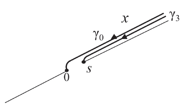
(b)

Figure 3. Crosscuts and contours: (a) shows the crosscuts and (b) shows the contours of the integrals, $\gamma_{a}=\gamma_{\infty,B_{a}}$ $(a=0,3)$.

We have the integrals along the contours from $\infty$ to $B_{a}$ denoted by $\gamma_{a}:=\gamma_{\infty,B_{a}}$; $\gamma_{0}$ and $\gamma_{3}$ are displayed in Figure 3 (b) as in Appendices A and B.

The integrals $\displaystyle{\omega_{X_{s}i,a}=\int_{\gamma_{a}}{\nu^{I}_{X_{s}i}}}$ $(i=1,2,3,a=0,1,2,3)$ are evaluated as follows.

Lemma 4.3.

The matrix of integrals has the expression,

$$\begin{pmatrix}\omega_{X_{s}1,0}&\omega_{X_{s}1,1}&\omega_{X_{s}1,2}&\omega_{X_{s}1,3}\\ \omega_{X_{s}2,0}&\omega_{X_{s}2,1}&\omega_{X_{s}2,2}&\omega_{X_{s}2,3}\\ \omega_{X_{s}3,0}&\omega_{X_{s}3,1}&\omega_{X_{s}3,2}&\omega_{X_{s}3,3}\end{pmatrix}=\begin{pmatrix}A^{(0)}_{10}&A^{(0)}_{11}&A^{(0)}_{12}&s^{-1/3}A^{(0)}_{13}\\ A^{(0)}_{20}&A^{(0)}_{21}&A^{(0)}_{22}&A^{(0)}_{23}\\ A^{(0)}_{30}&A^{(0)}_{31}&A^{(0)}_{32}&A^{(0)}_{33}\\ \end{pmatrix},$$

where $A^{(0)}_{ij}:=A^{(0)}_{ij}(s^{1/3})$ and $A^{(0)}_{ij}(t)$ are holomorphic functions with respect to $t=s^{1/3}$ such that

$$A^{(0)}_{13}(s=0)\neq 0.$$

Proof.

When we compute $\omega_{X_{s}a,b}$ $(a=1,2,3,b=1,2)$, we apply Lemma 4.2 since we can regard $\gamma_{a}$ $(a=1,2)$ as a subset of $V_{s}^{c}$. On the other hand the cases of $a=0$ and $a=3$ are in Lemmas B.2 and B.3 in Appendix B following Aomoto’s investigation in Appendix A. ∎

4.3. Periods for the degeneration

The following Lemmas 4.4 and 4.5 are corollaries of Lemma 4.3 by assuming $s\in D_{\varepsilon}^{*}$.

Lemma 4.4.

The matrices of the half-periods have the expression,

$$\omega^{\prime}_{X_{s}}=\begin{pmatrix}A^{(1)}_{11}&A^{(1)}_{12}&s^{-1/3}A^{(1)}_{13}\\ A^{(1)}_{21}&A^{(1)}_{22}&A^{(1)}_{23}\\ A^{(1)}_{31}&A^{(1)}_{32}&A^{(1)}_{33}\\ \end{pmatrix},\quad\omega^{\prime\prime}_{X_{s}}=\begin{pmatrix}s^{-1/3}A^{(2)}_{11}&A^{(2)}_{12}&s^{-1/3}A^{(2)}_{13}\\ A^{(2)}_{21}&A^{(2)}_{22}&A^{(2)}_{23}\\ A^{(2)}_{31}&A^{(2)}_{32}&A^{(2)}_{33}\\ \end{pmatrix},$$

where $A^{(a)}_{ij}:=A^{(a)}_{ij}(s^{1/3})$ and $A^{(a)}_{ij}(t)$ are holomorphic functions with respect to $t=s^{1/3}$ such that $A^{(a)}_{13}(0)$ $(a=1,2)$ and $A^{(2)}_{11}(0)$ are not zero.

Proof.

In the computation, we note that the contours of $\gamma_{a}$ $(a=0,3)$ shown in Figure 1 are given as Figure 3. Due to Lemmas 2.3, 4.2, 4.3, and the fact that $\gamma_{a}$ $(a=1,2)$ is a subset of $V_{s}^{c}$, we have the above results. Especially from (A.3), we have

$$A^{(1)}_{13}=\frac{\zeta_{3}^{2}}{\sqrt[3]{(b_{1}b_{2})^{2}}}\sum_{\ell=0}\beta^{(2)}_{\ell}s^{\ell}\frac{\Gamma(\ell+\frac{1}{3})\Gamma(\frac{1}{3})}{\Gamma(\ell+\frac{2}{3})}$$

using the notations in (A.3). ∎

Lemma 4.5.

The determinant $|\omega^{\prime}_{X_{s}}|=s^{-1/3}A(s^{1/3})$,

$$\omega^{\prime-1}_{X_{s}}=\begin{pmatrix}s^{1/3}A^{(3)}_{11}&A^{(3)}_{12}&A^{(3)}_{13}\\ s^{1/3}A^{(3)}_{21}&A^{(3)}_{22}&A^{(3)}_{23}\\ s^{1/3}A^{(3)}_{31}&s^{1/3}A^{(3)}_{32}&s^{1/3}A^{(3)}_{33}\\ \end{pmatrix},\quad\omega^{\prime-1}_{X_{s}}\omega^{\prime\prime}_{X_{s}}=\begin{pmatrix}A^{(4)}_{11}&A^{(4)}_{12}&A^{(4)}_{13}\\ A^{(4)}_{21}&A^{(4)}_{22}&s^{1/3}A^{(4)}_{23}\\ A^{(4)}_{31}&s^{1/3}A^{(4)}_{32}&A^{(4)}_{33}\\ \end{pmatrix},$$

where for $a=3,4$, $A^{(a)}_{ij}:=A^{(a)}_{ij}(s^{1/3})$ and $A^{(a)}_{ij}(t)$ and $A(t)$ are holomorphic functions with respect to $t=s^{1/3}$ such that $A(0)\neq 0$.

Proof.

The first relation is directly derived from Lemma 4.4. Thus we obtain the formula for $\omega^{\prime-1}_{X_{s}}$. Using it, we have

$$\omega^{\prime-1}_{X_{s}}\omega^{\prime\prime}_{X_{s}}=\begin{pmatrix}A^{(4)}_{11}&A^{(4)}_{12}&A^{(4)}_{13}\\ A^{(4)}_{21}&A^{(4)}_{22}&A^{(4)\prime}_{23}\\ A^{(4)}_{31}&s^{1/3}A^{(4)}_{32}&A^{(4)}_{33}\\ \end{pmatrix},$$

and the fact that $\omega^{\prime-1}_{X_{s}}\omega^{\prime\prime}_{X_{s}}$ is a symmetric matrix leads the third result. ∎

From Lemma 2.6, we have the following lemma:

Lemma 4.6.

$${\eta^{{\prime}}_{X_{s}}}=\begin{pmatrix}s^{1/3}A^{(5)}_{11}&s^{1/3}A^{(5)}_{12}&s^{1/3}A^{(5)}_{13}\\ A^{(5)}_{21}&A^{(5)}_{22}&A^{(5)}_{23}\\ A^{(5)}_{31}&A^{(5)}_{32}&A^{(5)}_{33}\\ \end{pmatrix},\quad{\eta^{{\prime\prime}}_{X_{s}}}=\begin{pmatrix}s^{1/3}A^{(6)}_{11}&s^{1/3}A^{(6)}_{12}&s^{1/3}A^{(6)}_{13}\\ A^{(6)}_{21}&A^{(6)}_{22}&A^{(6)}_{23}\\ A^{(6)}_{31}&A^{(6)}_{32}&A^{(6)}_{33}\\ \end{pmatrix},$$

where for $a=5,6$, $A^{(a)}_{ij}:=A^{(a)}_{ij}(s^{1/3})$ and $A^{(a)}_{ij}(t)$ and $A(t)$ are holomorphic functions with respect to $t=s^{1/3}$ such that $A(0)\neq 0$.

Proof.

The terms coupled with $\omega^{{\prime}}_{X_{s}13}$ in Lemma 2.6 should be finite due to the Legendre relation and they consist of ${\eta^{{\prime}}_{X_{s}1j}}$ for $j=1,2,3$. Thus ${\eta^{{\prime}}_{X_{s}}}$ behaves above and Lemma 2.3 determines the ${\eta^{{\prime\prime}}_{X_{s}}}$. ∎

4.4. The sigma function in terms of the al function

From (2.6) and (2.7), the discriminant $\Delta_{s}$ vanishes at $s\to 0$ whereas $c_{s}$ diverges.

Lemma 4.7.

At $s=0$, we have

$$\Delta_{s}=(-729b_{1}^{10}b_{2}^{10})s^{4}(1+d_{\geq 1}(s)),\quad c_{s}=\left(\frac{(2\pi)^{3}}{A(0)}\right)^{1/2}\frac{s^{-1/3}}{(-729b_{1}^{10}b_{2}^{10})^{1/8}}(1+d_{\geq 1}(s)),$$

where $d_{\geq n}(s)$ means formal series of $s$ whose degree is greater than or equal to $n$ in ${\mathbb{C}}[b_{1},b_{2}][[s]]$.

The recent investigation [7, 14] shows the result:

Proposition 4.8.

For every $s\in D_{s}$, the sigma function is expanded as

$${\sigma_{X_{s}}}(u)=u_{1}-u_{2}^{2}u_{3}+\mathrm{\mbox{higher-order terms with respect to the weight of $u$}}$$

at the origin of ${\mathbb{C}}^{3}$.

Remark 4.9.

Proposition 4.8 entails that the sigma function can be defined even for $X_{0}$. One of the reasons is that the Schur polynomial can be regarded as a sigma function of the monomial curve $Y^{3}=X^{4}$ [7, 14]. Proposition 4.8 and Lemma 4.7 imply that for the limit of $s\to 0$, the $c_{s}$ diverges whereas the theta function also vanishes to the order of $s^{1/3}$ and $\sigma$ is defined. Thus this property of the sigma function in Proposition 4.8 is very crucial. However the proposition only shows the local behavior of ${\sigma_{X_{s}}}$ at a point, or in the image of ${\widetilde{w}_{X_{s}}}$ for $\kappa_{X}^{-1}(\infty,\infty,\infty)$ in ${\mathcal{S}}^{3}{\widetilde{X}}_{s}$; this does not capture the degeneration phenomenon, and moreover, the argument of ${\sigma_{X_{{\widehat{0}}}}}$ is translated (cf. Subsection 3.5). We investigate instead the relation between ${\sigma_{X_{{\widehat{0}}}}}$ and ${\sigma_{X_{s}}}$ directly using the result in Proposition 4.8 and the $\mathrm{al}_{a}^{(c)}$-function in Proposition 2.9.

We now, evaluate the sigma function, ${\sigma_{X_{s}}}$ at the Abel-map image of the branch point $\displaystyle{\omega_{s}=\int_{\gamma_{3}}{\nu^{I}_{X_{s}}}}$ for $\gamma_{3}$ in Figure 3 using the $\mathrm{al}_{3}^{(0)}$-function.

Lemma 4.10.

For $P_{i}=(x_{i},y_{i})\in X_{s}$

$$x_{i}=\frac{1}{t_{i}^{3}},\quad y_{i}=\frac{1}{t_{i}^{4}}(1+d_{\geq 1}(t_{i})),$$

and $u^{(i)}={\widetilde{w}_{X_{s}}}{}(P_{i})$ $(i=1,2)$, we have the following relation,

$${\sigma_{X_{s}}}(u^{(1)}+u^{(2)}+\omega_{s})=-\frac{\sqrt{2}}{\sqrt[3]{b_{1}b_{2}}}s^{-1/3}t_{1}t_{2}(1+d_{\geq 1}(s,t_{1},t_{2},t_{3})).$$

Proof.

For $P_{3}\in X_{s}$ and $u^{(3)}={\widetilde{w}_{X_{s}}}{}(P_{3})$, let us consider

$$u=u^{(1)}+u^{(2)}+u^{(3)}+\omega_{s},$$

and the limit $u^{(3)}\to 0$ or $P_{3}\to\infty$. For the limit,

(4.2) $${{\sigma_{X_{s}}}(u+\omega_{s})=\frac{\sqrt{2}\mathrm{e}^{{}^{t}u\varphi_{s;0}}}{\sqrt[3]{s(s-b_{1})(s-b_{2})}}\mathrm{al}_{3}^{(0)}(u){\sigma_{X_{s}}}(u)}$$

is reduced to the above relation because a direct computation shows

$$\mathrm{al}_{3}^{(0)}(u)=\frac{1}{t_{1}^{2}+t_{1}t_{2}+t_{2}^{2}}\frac{1}{t_{3}}(1+d_{\geq 1}(s,t_{1},t_{2},t_{3}))$$

and due to Proposition 4.8,

$${\sigma_{X_{s}}}(u)=t_{1}t_{2}(t_{1}^{2}+t_{1}t_{2}+t_{2}^{2})t_{3}(1+d_{\geq 1}(s,t_{1},t_{2},t_{3})).$$

Note that the $\varphi_{s;0}$ of $\mathrm{e}^{{}^{t}u\varphi_{s;0}}$ does not have any effect on this evaluation. We can arrange for the ambiguous third root of unity to 1 by considering proper contours in the integral. ∎

4.5. The limit in $D_{\varepsilon}^{*}$ and $X_{\widehat{0}}$

Now we are ready to describe the behavior of $X_{s}$ for $s\to 0$ in $\pi_{\mathfrak{X}}^{-1}D_{s}^{*}$ and compare it with that of $X_{\widehat{0}}$ by using $x$-constant sections of $D_{\varepsilon}$. As we consider the $x$-constant section $P:D_{\varepsilon}\to\mathfrak{X}$ which is denoted by $P_{s}=(x_{s},y_{s})$ for a point $s\in D_{\varepsilon}$, we consider the element $P$ in $X_{\widehat{0}}$ via the commutative diagram,

      

i.e., $\pi_{1}(P_{s})=\pi_{1}(P_{0})={\widehat{\pi}}_{1}(P)=x\in{\mathbb{P}}$ for $s\in D_{\varepsilon}$ and $\pi_{2}(P_{0})={\widehat{\pi}}_{2}(P)$ of $P\in X_{\widehat{0}}$. We will fix this convention.

The following show that under the limit of $s\to 0$, some quantities of $\pi_{\mathfrak{X}}^{-1}D_{\varepsilon}^{*}\subset\mathfrak{X}$ corresponds to those of $X_{{\widehat{0}}}$ using the $x$-constant sections, whereas others don’t correspond to anything.

We have the following lemmas.

Lemma 4.11.

For the $x$-constant section $P_{s}$ whose $\pi_{1}(P_{s})=x$ belongs to the region $V_{s}^{c}$ and $\pi_{1}(P_{0})={\widehat{\pi}}_{1}(\hat{P})$ of $\hat{P}\in X_{\widehat{0}}$, we have the relations under the limit $s\to 0$,

$$\lim_{s\to 0}{\nu^{I}_{X_{s}i+1}}(P_{s})={\nu^{I}_{X_{{\widehat{0}}}i}}(\hat{P}),\quad\lim_{s\to 0}{\nu^{I}_{X_{s}i+1}}(P_{s})={\nu^{II}_{X_{{\widehat{0}}}i}}(\hat{P}),\quad(i=1,2).$$

Lemma 4.12.

The $A^{(1)}$’s in Lemma 4.4 and $A^{(3)}$’s in Lemma 4.5 satisfy the following relations under the max-norm of the matrices,

$$\lim_{s\to 0}\begin{pmatrix}A^{(1)}_{21}&A^{(1)}_{22}\\ A^{(1)}_{31}&A^{(1)}_{32}\\ \end{pmatrix}=\omega_{X_{{\widehat{0}}}}^{\prime},\quad\lim_{s\to 0}\begin{pmatrix}A^{(1)}_{21}&A^{(1)}_{22}\\ A^{(1)}_{31}&A^{(1)}_{32}\\ \end{pmatrix}=\omega_{X_{{\widehat{0}}}}^{\prime\prime},$$

$$\lim_{s\to 0}s^{1/3}|\omega_{X_{s}}^{\prime}|=A^{(1)}_{13}|\omega_{X_{{\widehat{0}}}}^{\prime}|,\quad\lim_{s\to 0}\begin{pmatrix}A^{(3)}_{12}&A^{(3)}_{13}\\ A^{(3)}_{22}&A^{(3)}_{23}\\ \end{pmatrix}=\omega_{X_{{\widehat{0}}}}^{\prime-1}.$$

Proof.

In the computation, we note that the contours in Figures 1 and 3 are consistent with those of $X_{{\widehat{0}}}$ in in Figure 2. ∎

This means that

$$\lim_{s\to 0}\omega^{{\prime}}_{X_{s}i+1,j}=\omega^{{\prime}}_{X_{{\widehat{0}}}i,j},\qquad\lim_{s\to 0}{\omega^{{\prime\prime}}_{X_{s}i+1,j}}={\omega^{{\prime\prime}}_{X_{{\widehat{0}}}i,j}}.$$

Similarly we have the relations for the integrals of the second kind.

Lemma 4.13.

1. $\displaystyle{\lim_{s\to 0}{\eta^{{\prime}}_{X_{s}i+1,j}}=\eta^{{\prime}}_{X_{{\widehat{0}}}i,j}}$ and $\displaystyle{\lim_{s\to 0}{\eta^{{\prime\prime}}_{X_{s}i+1,j}}={\eta^{{\prime\prime}}_{X_{{\widehat{0}}}i,j}}}$ for $i,j=1,2$, and

2. $\displaystyle{\lim_{s\to 0}{\eta^{{\prime}}_{X_{s}1,j}}=\lim_{s\to 0}{\eta^{{\prime\prime}}_{X_{s}1,j}}=0}$ for $j=1,2,3$.

From Lemmas 2.4 and 3.6, it is easy to obtain the limit of $\tau_{X_{s}}$:

Lemma 4.14.

$$\lim_{s\to 0}\tau_{X_{s}i,j}=\tau_{X_{\widehat{0}}i,j},\quad(i,j=1,2).$$

We show that the limit of the Riemann constant $\xi_{X_{s}}$ in (2.5) turns out to be the shifted Riemann constant $\xi_{X_{\widehat{0}}{\mathfrak{s}}}$ in (3.5); we analytically compute the limit of the theta characteristics $\delta_{X_{s}}$ is $\delta_{X_{\widehat{0}}}$; since the divisors at infinity correspond, we demonstrate naturalness of the shifted Riemann constant.

Proposition 4.15.

$$\lim_{s\to 0}\xi_{X_{s},j}=\xi_{X_{\widehat{0}},j}-{\widetilde{w}}_{X_{\widehat{0}},j}^{o}(\iota_{X}B_{0})=\xi_{X_{\widehat{0}}{\mathfrak{s}},j},\quad(j=1,2).$$

$$\delta^{\prime}_{X_{s},j}\longrightarrow\delta^{\prime}_{X_{\widehat{0}},j},\quad\delta^{\prime\prime}_{X_{s},j}\longrightarrow\delta^{\prime\prime}_{X_{\widehat{0}},j},\quad(j=1,2).$$

Proof.

For brevity, we omit $\iota_{X}$ in ${\widetilde{w}}_{X_{s},i}^{o}$ here. Let us consider the limit of $s\to 0$ of (2.5),

(4.3) $$\xi_{X_{s}j}=\frac{1}{2}\tau_{X_{s}jj}+\sum_{i=1}^{2}\int_{\alpha_{i}}{\widetilde{w}}_{X_{s},i}^{o}(P){\nu^{I\circ}_{X_{s}j}}(P)+\int_{\alpha_{3}}{\widetilde{w}}_{X_{s},3}^{o}(P){\nu^{I\circ}_{X_{s}j}}(P)+{\widetilde{w}}_{X_{s},j}^{o}(Q_{j}).$$

noting (3.4). Let the third term in the right hand side be denoted by $I$. For sufficiently small $s\in\Delta_{\varepsilon}^{*}$, let ${\widetilde{w}}_{X_{s},i}^{o}(P)={\widetilde{w}}_{X_{s},i}^{o}(B_{0})+w_{i}(z)$ using the local parameter $z$ of $x=z^{3}$ at $B_{0}$. Though $w_{3}(z)$ is a linear combination of $({\widetilde{w}}_{X_{s},i}(P)-{\widetilde{w}}_{X_{s},i}(B_{0}))$’s, the dominant term of $w_{3}(z)$ at $B_{0}$ is $\displaystyle{\int_{0}^{P}{\nu^{I}_{X_{s}1}}}$. Since $\displaystyle{{\nu^{I}_{X_{s}1}}=\frac{dz}{z^{2}}(1+d_{\geq 1}(z))}$ and other entries are holomorphic at $B_{0}$, the partial integration at $s=0$ gives

$$I=\oint_{\alpha_{3}}(w_{3}(z)dw_{j}(z))=-\oint_{\alpha_{3}}(dw_{3}(z)(w_{j}(z)+{\widetilde{w}}_{X_{s},j}^{o}(B_{0})))=-{\widetilde{w}}_{X_{s},j}^{o}(B_{0}).$$

Since $\displaystyle{\oint_{\alpha_{3}}dw_{3}(z)=1}$, the third equality implies $\displaystyle{I^{\prime}:=\oint_{\alpha_{3}}dw_{3}(z)w_{j}(z)\to 0}$ for $s\to 0$, which we now show.

Let $\displaystyle{w_{j}(z)=\sum_{i=1}^{\infty}a^{(j)}_{i}z^{i}}$ noting $w_{j}(0)=0$; it has non-vanishing radius of convergence. On the other hand, at $s=0$, $\displaystyle{dw_{3}(z)=\frac{s^{1/3}}{A_{13}^{(1)}}{\nu^{I}_{X_{s}1}}(1+d_{\geq 1}(s^{1/3}))}$. As in Appendix A, we assume $s$ to be positive without loss of generality. Using the notations in (A.3),

$$\begin{split}I^{\prime}&=\frac{(\zeta_{3}^{2}-\zeta_{3})s^{1/3}}{A_{13}^{(1)}}\int^{s}_{0}\frac{h_{2}(x)w_{j}(x^{1/3})}{\sqrt[3]{|x^{2}(x-s)^{2}|}}dx+d_{\geq 2}(s^{1/3})\\ &=\frac{(\zeta_{3}^{2}-\zeta_{3})}{A_{13}^{(1)}}\frac{\zeta_{3}^{2}}{\sqrt[3]{(b_{1}b_{2})^{2}}}\sum_{\ell=0}\sum_{n=1}\beta^{(2)}_{\ell}a^{(j)}_{n}s^{\ell+n/3}\int^{1}_{0}t^{\ell+\frac{n+1}{3}-1}(1-t)^{\frac{1}{3}-1}dt+d_{\geq 2}(s^{1/3}).\end{split}$$

Thus it is obvious that $\displaystyle{\lim_{s\to 0}I^{\prime}=0}$. The other terms in (4.3) becomes $\xi_{X_{\widehat{0}},j}$ and thus we show the proposition. ∎

Now let us consider the limit of $s\to 0$ of $\mathcal{J}_{s}$.

Remark 4.16.

For $s\to 0$, the rank of the matrix $\omega_{X_{3}}^{\prime-1}$ is reduced to two. This implies that for $s\to 0$, we have a 2-dimensional space, hence every vector is a combination of two vectors and

$${\mathbb{C}}^{3}\ni\omega^{\prime-1}_{X_{s}}\begin{pmatrix}u_{1}\\ u_{2}\\ u_{3}\end{pmatrix}\longrightarrow\begin{pmatrix}z_{0}+s^{1/3}A^{(3)}_{11}u_{1}\\ z_{1}+s^{1/3}A^{(3)}_{21}u_{1}\\ s^{1/3}z_{2}+s^{1/3}A^{(3)}_{31}u_{1}\end{pmatrix}\in{\mathbb{C}}^{3},$$

for certain $z$’s. However Proposition 4.8 and Remark 4.9 mean that by rescaling $u_{1}$ in each component of the image of $\omega^{\prime-1}_{X_{s}}$, $u_{1}$ survives in the expansion of the sigma function and contributes to the expression in Proposition 4.8.

For $s\in D_{\varepsilon}^{*}$, let us consider the image of

$${\widetilde{w}_{X_{s}\mathfrak{s}}}{}:{\mathcal{S}}^{2}{\widetilde{X}}_{s}\to{\mathbb{C}}^{3},\quad{\widetilde{w}_{X_{s}\mathfrak{s}}}{}(\gamma_{1},\gamma_{2}):={\widetilde{w}_{X_{s}}}{}(\gamma_{1},\gamma_{2},\iota_{X}(B_{s})),$$

and consider the projections $p_{2,3}:{\mathbb{C}}^{3}\to{\mathbb{C}}^{2}$ and $p_{2,3}^{\perp}:{\mathbb{C}}^{3}\to{\mathbb{C}}$ such that $p_{2,3}(u_{1},u_{2},u_{3})=(u_{2},u_{3})$ and $p_{2,3}^{\perp}(u_{1},u_{2},u_{3})=(u_{1})$.

Proposition 4.17.

The map $(p_{2,3}{\widetilde{w}_{X_{s}\mathfrak{s}}}{})$ is well-defined even for the limit $s\to 0$. The image of $\lim_{s\to 0}(p_{2,3}{\widetilde{w}_{X_{s}\mathfrak{s}}}{})$ is ${\mathbb{C}}^{2}$.

Proof.

It is obvious that $p_{2,3}{\widetilde{w}_{X_{s}\mathfrak{s}}}{}$ agrees with ${\widetilde{w}_{X_{{\widehat{0}}}\mathfrak{s}}}$ for the limit $s\to 0$ due to Lemmas 4.11 and 4.12. The Abel-Jacobi theorem for $X_{\widehat{0}}$ shows that the image of ${\widetilde{w}_{X_{{\widehat{0}}}\mathfrak{s}}}$ is ${\mathbb{C}}^{2}$. ∎

We state our main theorem.

Theorem 4.18.

For every $v={}^{t}(v_{1},v_{2})\in{\mathbb{C}}^{2}$, there are $x$-constant sections $\gamma_{1}$ and $\gamma_{2}$ of ${\mathcal{H}}^{0}(D_{\varepsilon}^{*},{\mathcal{S}}^{2}{\widetilde{\mathfrak{X}}})$, such that

$$v=\lim_{s\to 0}p_{2,3}{\widetilde{w}_{X_{s}\mathfrak{s}}}{}(\gamma_{1},\gamma_{2}),$$

and $u={\widetilde{w}_{X_{s}\mathfrak{s}}}{}(\gamma_{1},\gamma_{2})(={\widetilde{w}_{X_{s}}}{}(\gamma_{1},\gamma_{2})+\omega_{s})$, we have the relation,

(4.4) $$\sigma_{X_{{\widehat{0}}}}(v)=\lim_{s\to 0}\left(\frac{\sqrt[3]{sb_{1}b_{2}}}{\sqrt{2}}{\sigma_{X_{s}}}(u)\right).$$

Proof.

The first equation is obtained by the Abel theorem for ${\widetilde{X}}_{{\widehat{0}}}$ and Proposition 4.17. Noting $u={\widetilde{w}_{X_{s}}}{}(\gamma_{1},\gamma_{2})+\omega_{s}$, Proposition 3.7 (v), and Lemma 4.10, the expansions of both sides at the origin in ${\mathbb{C}}^{2}$ agree. On the other hand, the translational formula of ${\sigma_{X_{s}}}$ of $X_{s}|_{s=0}$ on $(u_{1},u_{2}+\ell_{2},u_{3}+\ell_{3})$ for ${}^{t}(\ell_{2},\ell_{3})\in p_{2,3}\Gamma_{s}|_{s=0}$ agrees with that of ${\sigma_{X_{{\widehat{0}}}}}$ on $(v_{1}+\ell_{2},v_{2}+\ell_{3})$ for ${}^{t}(\ell_{2},\ell_{3})\in\Gamma_{\widehat{0}}=p_{2,3}\Gamma_{s}|_{s=0}$ because of Lemmas 4.12, 4.13 and 4.14 and Propositions 3.7 (3) and 4.15. ∎

Remark 4.19.

The factor $s^{1/3}$ of the right-hand side in (4.4) means that the function is well defined on a triple cover $\widetilde{D_{\varepsilon}^{*}}$ of $D_{\varepsilon}^{*}$. This corresponds to the group action $\widehat{\zeta}_{3}^{*}$ in Lemma 3.1. Corresponding to the group action $\widehat{\zeta}_{3}^{*}$, i.e., $X_{{\widehat{0}}}^{*}=\widehat{\zeta}_{3}^{*}X_{{\widehat{0}}}$ and $X_{{\widehat{0}}}^{**}=\widehat{\zeta}_{3}^{*2}X_{{\widehat{0}}}$, the left-hand side of ${\sigma_{X_{{\widehat{0}}}}}$ of $X_{{\widehat{0}}}$ in (4.4) is replaced with the sigma functions $\sigma_{X_{{\widehat{0}}}^{*}}$ and $\sigma_{X_{{\widehat{0}}}^{**}}$ of $X_{{\widehat{0}}}^{*}$ and $X_{{\widehat{0}}}^{**}$ rather than $X_{\widehat{0}}$.

On the other hand, since the factor $s^{1/3}$ in the right hand side in (4.4) comes from $f^{\prime}(b_{s})$ in Proposition 2.9 and the proof of Lemma 4.10, this action $\widehat{\zeta}_{3}^{*}$ can be regarded as the action $\widehat{\zeta}_{3}^{\prime}$ on the triple covering of the domain of the $\mathrm{al}$ function (2.9) in the limit of the degenerating family of curves because $z$ in $X_{\widehat{0}}$ and $\mathrm{al}_{3}^{(0)}$ in $X_{0}$ are the local parameters of the branch points $(B_{X_{\widehat{0}},0})$ and $\pi_{al,3}^{-1}(B_{s})$. The symmetries $\widehat{\zeta}_{3}^{*}$ and $\widehat{\zeta}_{3}^{\prime}$ act on these local parameters. After $B_{s}$ and $B_{0}$ collapse, Theorem 4.18 shows the identification of $\widehat{\zeta}_{3}^{\prime}$ with $\widehat{\zeta}_{3}^{*}$.

Accordingly, by introducing ${\widetilde{w}_{X_{s}\mathfrak{s}}}{}^{(c)}(\gamma_{1},\gamma_{2}):={\widetilde{w}_{X_{s}}}{}(\gamma_{1},\gamma_{2})+\widehat{\zeta}_{3}^{c}\omega_{s}$ for $c=0,1,2$ and using the expansions of $\mathrm{al}_{3}^{(c)}$, we have other versions of the sigma function as the left hand side in (4.4) under the action of $\widehat{\zeta}_{3}^{\prime}$. We encounter three sigma functions

(4.5) $$\sigma_{X_{\hat{0}}}(v),\quad\sigma_{X_{\hat{0}}^{*}}(v),\quad\sigma_{X_{\hat{0}}^{**}}(v)\quad$$

of three curves of genus two as in Subsection 3.7.

Remark 4.20.

In Appendix C, we investigate the behavior of the Weierstrass sigma function of the degenerating family of the elliptic curves $y(y-s)=x^{3}$ for $s\to 0$, which behaves similarly to the sigma function for $X_{s}$. We make some remarks on this comparison.

We note that ${}^{t}u\varphi_{s;0}$ in the proof of Lemma 4.10 is decomposed to ${}^{t}u\varphi_{s;0}=p_{2,3}^{\perp}({}^{t}u\varphi_{s;0})+$ $p_{2,3}({}^{t}u\varphi_{s;0})$ by letting $p_{2,3}^{\perp}({}^{t}u\varphi_{s;0}):=u_{1}\varphi_{s;0,1}$ and $p_{2,3}({}^{t}u\varphi_{s;0}):=u_{2}\varphi_{s;0,2}+u_{3}\varphi_{s;0,3}$ and in the genus one case, $\mathrm{e}^{\varphi_{0}u}$ behaves like the sigma function of ${\mathbb{P}}$, cf. Proposition C.12 and Remark C.13. Further the quasi-periodicity of the sigma function $\sigma(u+\omega_{s})$ in the left hand side of (4.2) for the image of $p_{2,3}$ is determined by $\mathrm{e}^{p_{2,3}({}^{t}u\varphi_{s;0})}$, $\mathrm{al}$-function and $\sigma(u)$. Though due to Lemma 4.13, $\eta_{1j}^{\prime}$ and $\eta_{1j}^{\prime\prime}$ $(j=1,2,3)$ in $\varphi_{s;0,1}$ become zero for the limit $s\to 0$, we can rewrite the relation (4.4) in Theorem 4.18 at $s=0$ as

(4.6) $${\sigma_{X_{s}}}(u)=\frac{\sqrt{2}\mathrm{e}^{p_{2,3}^{\perp}({}^{t}u\varphi_{s;0})}}{\sqrt[3]{sb_{1}b_{2}}}\sigma_{X_{{\widehat{0}}}}(p_{2,3}(u))(1+d_{>0}(s^{1/3}))$$

for $u={\widetilde{w}_{X_{s}}}{}(\gamma_{1},\gamma_{2})+\omega_{s}$ and $x$-constant sections $\gamma_{1}$, $\gamma_{2}$ $\in{\mathcal{H}}^{0}(D_{\varepsilon}^{*},{\mathcal{S}}^{2}{\widetilde{\mathfrak{X}}})$, where $d_{>0}(s^{1/3})$ means a formal power series in $s^{1/3}$ with certain coefficients. For the parameter $t=\omega^{{\prime}-1}_{X_{s}}u$ ($u=\omega^{{\prime}}_{X_{s}}t$), $\mathrm{e}^{p_{2,3}^{\perp}({}^{t}t{}^{t}\omega^{{\prime}}_{X_{s}}\varphi_{s;0})}$ is the sigma function of ${\mathbb{P}}$ for the limit $s\to 0$ as in Remark C.13. The expression (4.6) is consistent with the generalized theta function [9, 17, 16].

Further from (3.7), (4.5) is regarded as the sigma function $\sigma_{X_{\hat{0}}}$ with the actions $(\widehat{\zeta}_{3}^{*})^{0}$, $\widehat{\zeta}_{3}^{*}$ and $(\widehat{\zeta}_{3}^{*})^{2}$. On the other hand, on the normalization of the curve the action $\widehat{\zeta}_{3}^{*}$ is represented by the action $\widehat{\zeta}_{3}^{*}:z\mapsto\zeta_{3}z$ on the rational curve ${\mathbb{P}}$ as in Lemma 3.1 and Remark 3.2. Thus we can interpret (4.5) as the sigma function of the curve $X_{\hat{0}}$ of genus two and two actions $\widehat{\zeta}_{3}^{*}$ on two rational curves ${\mathbb{P}}$’s; their union can be viewed as the singular fiber in this degenerating family $\mathfrak{X}$. This interpretation corresponds to (C.9) in Remark C.13.

Remark 4.21.

It should be emphasized that Theorem 4.18 provides the algebraic and analytic properties of the sigma function of the normalized curve of singular fiber in the degenerating family $\mathfrak{X}$ as the limit of ${\sigma_{X_{s}}}$. This is an essentially new step, since the algebraic and analytic properties of the sigma function, (e.g., addition theorem, the Galois action, dependence on moduli parameters via the heat equation) have received much attention [10, 13, 14, 26, 27] for the case of (planar) $(n,s)$ curves, including $X_{s}$. Theorem 4.18 determines how these algebraic and analytic properties behave for ${\sigma_{X_{{\widehat{0}}}}}$ of $X_{\widehat{0}}$, which cannot be of $(n,s)$ type (its Weierstrass semigroup is non-symmetric). Due to Theorem 4.18, it is obvious that some of the properties of ${\sigma_{X_{s}}}$ survive. For example, the power expansion of the sigma function of $X_{s}$ is explicitly given by Nakayashiki and Ônishi [29, 33]; Theorem 4.18 and (4.2) provide the power expansion of $\sigma_{X_{{\widehat{0}}}}(v)$ explicitly. As another example, Theorem 4.18 and (4.2) lead the addition theorem and $n$-division formulae for ${\sigma_{X_{s}}}$ [31] to those of $\sigma_{X_{{\widehat{0}}}}$, a non-planar curve.

Further Theorem 4.18 and above remarks show that the Galois actions $\widehat{\zeta}_{3}$ and $\widehat{\zeta}_{3}^{\prime}$ on our cyclic curves $X_{s}$ play an essential role in their degenerations. Theorem 4.18 can be generalized to the sigma functions of cyclic trigonal curves $y^{3}=f(x)$ whose Weierstrass semigourp is generated by $(3,p)$ since we also constructed the sigma functions of the space curves of $(3,p,q)$-type whose Weierstrass semigroup is generated by $(3,p,q)$ [22]; our investigations in this paper correspond to the simplest case $(p,q)=(4,5)$.

Lastly, in [32], Ônishi investigated the more general Galois action on the sigma function for the trigonal curves of the Weierstrass canonical form $y^{3}+(\mu_{2}x+\mu_{5})y^{2}+(\mu_{1}x+\mu_{4}x^{2}+$ $\mu_{7}x+\mu_{10})y+x^{5}+\mu_{3}x^{4}+\mu_{6}x^{3}+\mu_{9}x^{2}+\mu_{12}x+\mu_{15}=0$ of genus four rather than a cyclic trigonal curve $X_{s}$; his result is easily modified to the curve of genus three. Using the results in [32], the above actions $\widehat{\zeta}_{3}$, $\widehat{\zeta}_{3}^{\prime}$ and $\widehat{\zeta}_{3}^{*}$ can be extended to more general Galois actions. Thus our investigations could be generalized for a degenerating family of plane curves in Weierstrass canonical form as mentioned in [20, 21].

Remark 4.22.

The behavior of these sigma function could be explicitly compared with the generalized theta function for the same limit [16].

A. Appendix: Integrals by Kazuhiko Aomoto

In this appendix, we assume that $s$ is a positive sufficiently small real number satisfying $0<s<\delta<\min\{|b_{1}|,|b_{2}|\}$. Further, without loss of generality, the imaginary parts of $b_{1}$ and $b_{2}$ are positive, i.e., $Im(b_{1})>s$ and $Im(b_{2})>s$. Let

$$h_{2}(x):=\frac{1}{\sqrt[3]{(x-b_{1})^{2}(x-b_{2})^{2}}}$$

such that $\displaystyle{h_{2}(0)=\frac{\zeta_{3}^{2}}{\sqrt[3]{(b_{1})^{2}(b_{2})^{2}}}}$ and we choose the branch so that $\sqrt[3]{x^{2}(x-s)^{2}}$ should be positive for $[x,\infty)$. Using $h_{2}(x)$, we consider two integrals for $[0,\infty)$ and $(s,\infty)$,

$$I_{1}(s):=\int^{\infty}_{0}\frac{h_{2}(x)}{\sqrt[3]{x^{2}(x-s)^{2}}}dx,\quad I_{2}(s):=\int^{\infty}_{s}\frac{h_{2}(x)}{\sqrt[3]{x^{2}(x-s)^{2}}}dx.$$

More precisely, $I_{1}$ is defined as the upper half part of the contour integral with a positive $\varepsilon\to 0$,

$$I_{1}(s)=\lim_{\varepsilon\to 0}\frac{1}{\xi_{3}-1}\int_{\gamma_{\varepsilon}}\frac{h_{2}(x)}{\sqrt[3]{x^{2}(x-s)^{2}}}dx,$$

which is illustrated in Figure A.1.

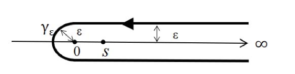
Figure A.1. The contour: The contour $\gamma_{\varepsilon}$ of the integral is illustrated.

Then we have the following proposition.

Proposition A.1.

When $\min\{|b_{1}|,|b_{2}|\}>s>0$, $Im(b_{1})>s$, and $Im(b_{2})>s$,

$$I_{1}(s)=f(s),\quad I_{2}(s)=s^{-1/3}g(s^{1/3}),$$

where $f(t)$ and $g(t)$ are regular functions with respect to $t$ in the region

$$U_{\epsilon}:=\{t\in{\mathbb{R}}\ |0\leq t<\epsilon\},$$

for a certain $\epsilon>0$ and $g(t)|_{t=0}\neq 0$.

We prove this proposition as follows. First we note that the assumptions $Im(b_{1})>0$ and $Im(b_{2})>0$ mean that $b_{a}$ $(a=1,2)$ does not belong to the $x$-axis.

It is obvious that $h_{2}(x)$ is holomorphic at $x=0$ and, as in (4.1) its expansion given by

$$h_{2}(x)=\frac{\zeta_{3}^{2}}{\sqrt[3]{b_{1}^{2}b_{2}^{2}}}\left(\sum_{i=0}^{\infty}\beta^{(2)}_{i}x^{i}\right),\quad\beta^{(2)}_{0}=1,$$

converges in $V_{b}:=\{x\in{\mathbb{C}}\ |\ |x|<\min\{|b_{1}|,|b_{2}|\}\}$. There is a certain neighborhood $V$ of ${\mathbb{R}}_{\geq 0}:=\{x\in{\mathbb{R}}\ |\ x\geq 0\}$ in the complex plane ${\mathbb{C}}$ such that

$$\Phi(x,s):=\frac{h_{2}(x)}{\sqrt[3]{x^{2}(x-s)^{2}}}$$

is a holomorphic function in $V\setminus{\mathbb{R}}_{\geq 0}$. Using a positive parameter $\rho$ ($\min(Im(b_{1}),Im(b_{2}))>\rho>$ $|s|>0$), we redefine the contour $\gamma\subset V$ $\gamma:(-\infty,\infty)\to{\mathbb{C}}$, given by

$$\gamma(t)=\left\{\begin{matrix}-t-{\displaystyle\frac{1}{2}}+\rho{\sqrt{-1}}&t\in\left(-\infty,-{\displaystyle\frac{1}{2}}\right],\\ \rho\mathrm{e}^{\pi(t+1){\sqrt{-1}}}&t\in\left(-{\displaystyle\frac{1}{2}},{\displaystyle\frac{1}{2}}\right],\\ t-{\displaystyle\frac{1}{2}}+\rho{\sqrt{-1}}&t\in\left({\displaystyle\frac{1}{2}},\infty\right)\end{matrix}\right.$$

illustrated in Figure A.2. $\gamma$ is disjoint to the points $b_{1}$ and $b_{2}$ in ${\mathbb{C}}$. Since $\gamma$ is homotopic to $\gamma_{\varepsilon}$, we show the proposition for the integrals of $\gamma$.

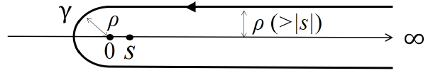
Figure A.2. The contour: The contour $\gamma$ of the integral is illustrated.

In view of the multi-valued property of $\Phi(x,s)$, the Cauchy integral theorem gives

(A.1) $$\begin{split}\int_{\gamma}\Phi(x,s)dx&=(\zeta_{3}-1)\int_{s}^{\infty}\frac{h_{2}(x)}{\sqrt[3]{x^{2}(x-s)^{2}}}dx+(-\zeta_{3}+1)\int_{0}^{s}\frac{h_{2}(x)}{|\sqrt[3]{x^{2}(x-s)^{2}}|}dx\\ &=:(\zeta_{3}-1)I_{\gamma}(s).\end{split}$$

Since $\gamma$ is disjoint with $[0,s]$ and $\{b_{1},b_{2}\}$ for $|s|<\rho$, $\Phi(x,s)$ is a regular function with respect to $(x,s)\in\gamma\times[0,\delta)$.

For the region, we have the expansion due to the absolute convergence,

$$\frac{1}{\sqrt[3]{(x-s)^{2}}}=\frac{1}{x^{2/3}}\left(\sum_{\ell=0}\frac{(3\ell+2)!!!}{\ell!}\left(\frac{2}{3}\frac{s}{x}\right)^{\ell}\right)=:\frac{1}{x^{2/3}}\sum_{\ell=0}c^{(2)}_{\ell}\left(\frac{s}{x}\right)^{\ell},$$

where $(3\ell+2)!!!=(3\ell+2)(3\ell-1)\cdots 5\cdot 2$.

$$\Phi(x,s)=\Phi(x,0)\left(1+\sum_{\ell=1}c^{(2)}_{\ell}\left(\frac{s}{x}\right)^{\ell}\right),$$

and

$$\Phi(x,0)=\frac{1}{\sqrt[3]{x^{4}(x-b_{1})^{2}(x-b_{2})^{2}}}.$$

Lemma A.2.

$\displaystyle{\int_{\gamma}\Phi(x,s)dx}$ is a regular function with respect to $s$, i.e., the power expansion

$$I_{\gamma}(s)=\int_{\gamma}\Phi(x,s)dx=\sum_{i=0}v_{i}s^{i},$$

has a finite radius of convergence $\delta^{\prime}$, where

$$v_{0}:=\int_{\gamma}\frac{1}{\sqrt[3]{x^{4}(x-b_{1})^{2}(x-b_{2})^{2}}}dx.$$

Since $\gamma_{\varepsilon}$ is homotopic to $\gamma$, we conclude that $I_{1}(s)=I_{\gamma}(s)/(\zeta_{3}-1)$.

On the other hand, from the definition, we obtain

(A.2) $$\begin{split}I_{1}(s)&=\int^{s}_{0}\frac{h_{2}(x)}{3\sqrt[3]{|x^{2}(x-s)^{2}|}}dx+I_{2}(s).\end{split}$$

It means that $I_{2}(s)$ is represented as the difference between the integrals over the generalized Lefschetz cycle and the detoured cycle,

$$I_{2}(s)=A_{2}-A_{1},$$

$$A_{1}=\int^{s}_{0}\frac{h_{2}(x)}{\sqrt[3]{|x^{2}(x-s)^{2}|}}dx,\quad A_{2}=\frac{1}{\zeta_{3}-1}\ \int_{\gamma}\Phi(x,s)dx.$$

By exchanging $x=st$, we have

(A.3) $$\begin{split}A_{1}&=\int^{s}_{0}\frac{h_{2}(x)dx}{\sqrt[3]{|x^{2}(x-s)^{2}|}}=\frac{\zeta_{3}^{2}}{\sqrt[3]{(b_{1}b_{2})^{2}}}\sum_{\ell=0}\beta^{(2)}_{\ell}\int^{s}_{0}\frac{x^{\ell}dx}{\sqrt[3]{|x^{2}(x-s)^{2}|}}\\ &=s^{-1/3}\frac{\zeta_{3}^{2}}{\sqrt[3]{(b_{1}b_{2})^{2}}}\sum_{\ell=0}\beta^{(2)}_{\ell}\int^{1}_{0}\frac{(st)^{\ell}dt}{\sqrt[3]{|t^{2}(t-1)^{2}|}}\\ &=s^{-1/3}\frac{\zeta_{3}^{2}}{\sqrt[3]{(b_{1}b_{2})^{2}}}\sum_{\ell=0}\beta^{(2)}_{\ell}s^{\ell}\int^{1}_{0}t^{\ell+\frac{1}{3}-1}(1-t)^{\frac{1}{3}-1}dt\\ &=s^{-1/3}\frac{\zeta_{3}^{2}}{\sqrt[3]{(b_{1}b_{2})^{2}}}\sum_{\ell=0}\beta^{(2)}_{\ell}s^{\ell}\frac{\Gamma(\ell+\frac{1}{3})\Gamma(\frac{1}{3})}{\Gamma(\ell+\frac{2}{3})}.\end{split}$$

We note that the series converges absolutely because, there is $0<c<1$ such that the ratio

(A.4) $$\left|\beta^{(2)}_{\ell+1}\frac{\Gamma(\ell+\frac{4}{3})\Gamma(\frac{1}{3})}{\Gamma(\ell+\frac{5}{3})}\frac{1}{\beta^{(2)}_{\ell}}\frac{\Gamma(\ell+\frac{2}{3})}{\Gamma(\ell+\frac{1}{3})\Gamma(\frac{1}{3})}\right|=\left|\frac{\beta^{(2)}_{\ell+1}}{\beta^{(2)}_{\ell}}\frac{\ell+\frac{4}{3}}{\ell+\frac{5}{3}}\right|$$

is smaller than $c$ for a certain $L$ and $\ell>L$. Further it is obvious that the leading term is not equal to zero, i.e.,

$$\frac{\zeta_{3}^{2}}{\sqrt[3]{(b_{1}b_{2})^{2}}}\beta^{(2)}_{0}\frac{\Gamma(\frac{1}{3})\Gamma(\frac{1}{3})}{\Gamma(\frac{2}{3})}\neq 0.$$

On the other hand, the second term $A_{2}$ is given by

$$\sum_{\nu=0}^{\infty}u_{\nu}s^{\nu},\quad u_{0}:=\frac{1}{\zeta_{3}-1}\int_{\gamma}\frac{1}{\sqrt[3]{x^{4}(x-b_{1})^{2}(x-b_{2})^{2}}}dx.$$

Then we obtain

$$I_{2}(s)=\sum_{\nu=0}^{\infty}u_{\nu}s^{\nu}-s^{-1/3}\frac{\zeta_{3}^{2}}{\sqrt[3]{(b_{1}b_{2})^{2}}}\sum_{\ell=0}\beta^{(2)}_{\ell}s^{\ell}\frac{\Gamma(\ell+\frac{1}{3})\Gamma(\frac{1}{3})}{\Gamma(\ell+\frac{2}{3})}.$$

It means the complete proof of the proposition.

Remark A.3.

The case when $s<0$ can be treated similarly, by replacing $I_{1}$ and $I_{2}$ with the corresponding integrals from $-\infty$ to $s$.

B. Appendix: Period Integrals

In this appendix, we apply the results in Appendix A by Aomoto to our integrals, $\omega_{X_{s}a,b}$. We assume that $s$ is a complex number such that $|s|\ll\min\{|b_{1}|,|b_{2}|\}$. We employ the contours in Figure 3. However the phase factor $\log(s/|s|)$ is not crucial since it correspond to rescaling the variables in the curve equation. Noting (4.1), we evaluate the integrals associated with the period matrices.

Lemma B.1.

There are regular functions $f_{a}(t)$ for $t\in V_{\epsilon}$ such that

$$\int^{s}_{0}{\nu^{I}_{X_{s}1}}=s^{-1/3}f_{1}(s^{1/3}),\quad\int^{s}_{0}{\nu^{I}_{X_{s}2}}=f_{2}(s^{1/3}),\quad\int^{s}_{0}{\nu^{I}_{X_{s}3}}=f_{3}(s^{1/3}),\quad$$

and $f_{1}(t)|_{t=0}$ does not vanish.

Proof.

From (A.3), we have the first relation. Similarly, we also have

$$\begin{split}\int^{s}_{0}{\nu^{I}_{X_{s}2}}&=\int^{s}_{0}\frac{h_{2}(x)xdx}{\sqrt[3]{x^{2}(x-s)^{2}}}=\frac{\zeta_{3}^{2}}{\sqrt[3]{(b_{1}b_{2})^{2}}}\sum_{\ell=0}\beta^{(2)}_{\ell}\int^{s}_{0}\frac{x^{\ell+1}dx}{\sqrt[3]{x^{2}(x-s)^{2}}}\\ &=s^{-1/3}\frac{\zeta_{3}^{2}}{\sqrt[3]{(b_{1}b_{2})^{2}}}\sum_{\ell=0}\beta^{(2)}_{\ell}\int^{1}_{0}\frac{(st)^{\ell+1}dt}{\sqrt[3]{t^{2}(t-1)^{2}}}\\ &=s^{2/3}\frac{1}{\sqrt[3]{(b_{1}b_{2})^{2}}}\sum_{\ell=0}\beta^{(2)}_{\ell}s^{\ell}\int^{1}_{0}t^{\ell+\frac{4}{3}-1}(1-t)^{\frac{1}{3}-1}dt\\ &=s^{2/3}\frac{1}{\sqrt[3]{(b_{1}b_{2})^{2}}}\sum_{\ell=0}\beta^{(2)}_{\ell}s^{\ell}\frac{\Gamma(\ell+\frac{4}{3})\Gamma(\frac{1}{3})}{\Gamma(\ell+\frac{5}{3})},\end{split}$$

$$\begin{split}\int^{s}_{0}{\nu^{I}_{X_{s}3}}&=\int^{s}_{0}\frac{h_{1}(x)xdx}{\sqrt[3]{x(x-s)}}=\frac{\zeta_{3}}{\sqrt[3]{(b_{1}b_{2})}}\sum_{\ell=0}\beta^{(1)}_{\ell}\int^{s}_{0}\frac{x^{\ell+1}dx}{\sqrt[3]{x^{2}(x-s)^{2}}}\\ &=s^{1/3}\frac{\zeta_{3}}{\sqrt[3]{(b_{1}b_{2})}}\sum_{\ell=0}\beta^{(1)}_{\ell}\int^{1}_{0}\frac{(st)^{\ell}dt}{\sqrt[3]{t(t-1)}}\\ &=s^{2/3}\frac{1}{\sqrt[3]{(b_{1}b_{2})}}\sum_{\ell=0}\beta^{(1)}_{\ell}s^{\ell}\int^{1}_{0}t^{\ell+\frac{2}{3}-1}(1-t)^{\frac{2}{3}-1}dt\\ &=s^{1/3}\frac{1}{\sqrt[3]{(b_{1}b_{2})}}\sum_{\ell=0}\beta^{(1)}_{\ell}s^{\ell}\frac{\Gamma(\ell+\frac{2}{3})\Gamma(\frac{2}{3})}{\Gamma(\ell+\frac{4}{3})}.\end{split}$$

Except the prefactor $s^{\ell}$, the series absolutely converge as in (A.4). ∎

Thus, we consider the integrals along the contours in Figure 3 (b). We have the following lemmas:

Lemma B.2.

There are regular functions $f^{\prime}_{a}(t)$ for $t\in V_{\epsilon}$ such that

$$\int_{\gamma_{3}}{\nu^{I}_{X_{s}1}}=s^{-1/3}f^{\prime}_{1}(s^{1/3}),\quad\int_{\gamma_{3}}{\nu^{I}_{X_{s}2}}=f^{\prime}_{2}(s^{1/3}),\quad\int_{\gamma_{3}}{\nu^{I}_{X_{s}3}}=f^{\prime}_{3}(s^{1/3}),\quad$$

and $f^{\prime}_{1}(t)|_{t=0}$ does not vanish.

Lemma B.3.

There are regular functions $g_{a}(t)$ for $t\in V_{\epsilon}$ such that

$$\int_{\gamma_{0}}{\nu^{I}_{X_{s}1}}=g_{1}(s^{1/3}),\quad\int_{\gamma_{0}}{\nu^{I}_{X_{s}2}}=g_{2}(s^{1/3}),\quad\int_{\gamma_{0}}{\nu^{I}_{X_{s}3}}=g_{3}(s^{1/3}).\quad$$

C. Appendix: The Weierstrass sigma function over the Kodaira IV degeneration

In this Appendix, we investigate the behavior of the Weierstrass sigma function of the degenerating family of the elliptic curves $y(y-s)=x^{3}$ $s\to 0$, which corresponds to type IV in the Kodaira classification of the degeneration of elliptic curves [19]. The main result in Proposition C.12 in this appendix can be compared to Theorem 4.18. Within this investigation, we introduce the al-function, which is the elliptic function version of the $\mathrm{al}$ function in Subsection 2.6 and [27]. The elliptic curve has the nongap sequence at $\infty$ determined by the numerical semigroup $\langle 3,2\rangle$.

C.1. Addition formula for the sigma function of $E_{s}:y(y-s)=x^{3}$

In [11], Eilbeck, Matsutani and Ônishi showed the following relation satisfied by the elliptic sigma function

(C.1) $$\frac{\sigma(u-v)\sigma(u-\zeta_{3}v)\sigma(u-\zeta_{3}^{2}v)}{\sigma(u)^{3}\sigma(v)^{3}}=(y(u)-y(v))$$

for the curve

$$y^{2}+\mu_{3}y=x^{3}+\mu_{6},$$

where $\zeta_{3}=\mathrm{e}^{2\pi{\sqrt{-1}}/3}$. We note that the formula holds for the sigma function of this particular curve because the curve has the symmetry of the trigonal cyclic action. The curve corresponds to the Weierstrass standard form,

$$(\wp^{\prime})^{2}=4\wp^{3}-g_{3}=4(\wp-e_{1})(\wp-e_{2})(\wp-e_{3}),$$

where $g_{3}=-4(\mu_{3}^{2}+\mu_{6})$ and $\wp(u)^{\prime}=2y+\mu_{3}$. Then we have

$$\sigma(\zeta_{3}u)=\zeta_{3}\sigma(u),\quad\wp(\zeta_{3}u)=\zeta_{3}\wp(u),\quad\wp^{\prime}(\zeta_{3}u)=\wp^{\prime}(u)$$

for $u\in{\mathbb{C}}$.

In this appendix, we specify the curve $E_{s}$,

$$y(y-s)=x^{3},\quad\left(y-\frac{s}{2}\right)^{2}=\left(x+\sqrt[3]{\frac{s^{2}}{4}}\right)\left(x+\zeta_{3}\sqrt[3]{\frac{s^{2}}{4}}\right)\left(x+\zeta_{3}^{2}\sqrt[3]{\frac{s^{2}}{4}}\right)$$

and its limit $s\to 0$, which corresponds to the type IV of the degeneration in Kodaira’s classification. Here $\mu_{3}=-s$, $\mu_{6}=0$, $\displaystyle{e_{j}=-\zeta_{3}^{1-j}\sqrt[3]{\frac{s^{2}}{4}}}$ $(j=1,2,3)$ and $g_{3}=-4s^{2}$.

In other words, we consider the degenerating family of $E_{s}$ for $D_{\varepsilon}:=\{s\in{\mathbb{C}}\ |\ |s|<\varepsilon\}$ and $D_{\varepsilon}^{*}=D_{\varepsilon}^{*}\setminus\{0\}$,

$${\mathfrak{E}}:=\{(x,y,s)\ |\ (x,y)\in E_{s},s\in D_{\varepsilon}\}$$

and $\pi_{{\mathfrak{E}}}:{\mathfrak{E}}\to D_{\varepsilon}$.

C.2. Elliptic integrals on $E_{s}$

We denote the integral from the point at infinity to $(x,y)=(0,s),$ by $\omega_{s}$, and that to $(0,0)$ by $\omega_{0}$,

$$\omega_{s}=\int^{(0,s)}_{\infty}du,\quad\omega_{0}=\int^{(0,0)}_{\infty}du,\quad du=\frac{dx}{2y-s}=\frac{dy}{3x^{2}}.$$

Further, the standard half-period integrals are given by [30],

(C.2) $$\omega^{\prime}=\omega_{1}=\int^{e_{1}}_{\infty}du,\quad\omega_{2}=\zeta_{3}^{2}\omega^{\prime},\quad\omega^{\prime\prime}=\omega_{3}=\zeta_{3}\omega^{\prime},$$

and

(C.3) $$\eta_{i}=\int_{\infty}^{e_{i}}xdu,\quad\eta^{\prime}=\eta_{1},\quad\eta^{\prime\prime}=\eta_{3}=\zeta_{3}^{2}\eta^{\prime}.$$

They satisfy the following

$$\omega_{1}+\omega_{2}+\omega_{3}=0,\quad\eta_{1}+\eta_{2}+\eta_{3}=0,\quad\eta^{\prime}\omega^{\prime\prime}-\eta^{\prime\prime}\omega^{\prime}=\frac{\pi{\sqrt{-1}}}{2},$$

and [30]

(C.4) $$\eta^{\prime}\omega^{\prime}=\frac{\pi{\sqrt{-1}}}{2(\zeta_{3}-\zeta_{3}^{2})}=\frac{\pi}{2\sqrt{3}}\in{\mathbb{R}}.$$

Using these, we define the lattice $\Gamma_{s}:={\mathbb{Z}}2\omega^{\prime}+{\mathbb{Z}}2\omega^{\prime\prime}$ [11]. Further the affine coordinates $(x,y)$ of the curve $E_{s}$ are written in terms of the $\wp$-function using the results in [11]:

$$\wp(u)=x(u),\quad\wp^{\prime}(u)=2y(u)-s,\quad y(u)=\frac{1}{2}(\wp^{\prime}(u)+s).$$

From [11], we have the expansions of $\sigma$ and $y$ for every $s\neq 0$:

Lemma C.1.

$$\sigma(u)=u-\frac{1}{120}s^{2}u^{7}+d_{\geq 11}(u),\qquad y(u)=-\frac{1}{u^{3}}+\frac{1}{2}s^{2}u^{3}+d_{\geq 9}(u).$$

Lemma C.2.

$$x(\zeta_{3}^{r}\omega_{s})=\wp(\zeta_{3}^{r}\omega_{s})=0,(r=0,1,2),\quad y(\omega_{0})=0,\quad y(\omega_{s})=s.$$

$$\omega_{0}=\frac{1-\zeta_{3}}{3}2\omega^{\prime},\quad\omega_{s}=\frac{1-\zeta_{3}^{2}}{3}2\omega^{\prime}=\frac{2+\zeta_{3}}{3}2\omega^{\prime}=\frac{2}{3}(2\omega^{\prime}+\omega^{\prime\prime}).$$

Proof.

The first three equations are obvious from [11]. We use the covering $\pi_{2}:E_{s}\to{\mathbb{P}}$ ($(x,y)\mapsto y$). We note that the $\omega_{s}$ is the contour integral from $\infty$ to $(0,s)$ and the point $(0,s)$ is a branch point. Thus when we consider the contour on another sheet of $\pi_{2}^{-1}$ as the return path from $(0,s)$ to $\infty$, we obtain a period and thus $(1-\zeta_{3})\omega_{s}$ must be a point in the lattice $\Gamma_{s}$. There exist $n$ and $m$ such that

$$(1-\zeta_{3})\omega_{s}=2\omega^{\prime}n+2\omega^{\prime\prime}m=2(n+\zeta_{3}m)\omega^{\prime}.$$

Thus we have

$$\omega_{s}=\frac{1}{3}(1-\zeta_{3}^{2})2(n+\zeta_{3}m)\omega^{\prime}.$$

We fix $\omega_{s}$ modulo $\Gamma_{s}$ and there are two possibilities

$$\omega_{s}=\pm\frac{1}{3}(1-\zeta_{3}^{2})2\omega^{\prime}\mbox{ modulo }\Gamma_{s}.$$

We find $\omega_{s}=\frac{1}{3}(1-\zeta_{3}^{2})2\omega^{\prime}$ numerically using Maple; in the other case we have $\omega_{0}$. ∎

Lemma C.3.

$$\omega^{\prime}=\frac{3}{2}\frac{1}{\zeta_{3}-\zeta_{3}^{2}}\frac{\Gamma\left(\frac{1}{3}\right)^{2}}{s^{1/3}\Gamma\left(\frac{2}{3}\right)},\quad\eta^{\prime}=\frac{\pi{\sqrt{-1}}}{3\sqrt{3}}\frac{s^{1/3}\Gamma\left(\frac{2}{3}\right)}{\Gamma\left(\frac{1}{3}\right)^{2}}.$$

Proof.

$\displaystyle{\omega_{s}-\omega_{0}=\int^{s}_{0}\frac{dy}{\sqrt[3]{y(y-s)}}}$ is given by $\displaystyle{\frac{\Gamma\left(\frac{1}{3}\right)^{2}}{s^{1/3}\Gamma\left(\frac{2}{3}\right)}}$ by putting $h(x)=1$ in (A.3). ∎

Then the action of the cyclic 3-group on $\omega_{s}$ and $\omega_{0}$ is given by the translation, which is illustrated in Figure C.3:

Lemma C.4.

$$\zeta_{3}\omega_{s}\equiv\omega_{s}-2\omega^{\prime},\quad\zeta_{3}^{2}\omega_{s}\equiv\omega_{s}-2(\omega^{\prime}+\omega^{\prime\prime})\mbox{ modulo }\Gamma_{s}.$$

Figure C.3. The points of $\omega_{0}$ and $\omega_{s}$ in the lattice $\Gamma_{s}$: The black dots show the points in $\Gamma_{s}$ whereas the white and the gray dots mean $\omega_{0}$ and $\omega_{s}$ modulo $\Gamma_{s}$ respectively. They have the translational symmetry.

The translation formula of the sigma function is given by [36]

(C.5) $$\sigma(u+2\omega^{\prime}n+2\omega^{\prime\prime}m)=(-1)^{n+m+nm}\mathrm{e}^{(2n\eta^{\prime}+2m\eta^{\prime\prime})(u+n\omega^{\prime}+m\omega^{\prime\prime})}\sigma(u).$$

and thus we have

(C.6) $$\sigma(u-\zeta_{3}\omega_{s})=\sigma(u-\omega_{s}+2\omega^{\prime})=(-1)\mathrm{e}^{2\eta^{\prime}(u+\omega_{s}+\omega^{\prime})}\sigma(u-\omega_{s}),$$

$$\sigma(u-\zeta_{3}^{2}\omega_{s})=\sigma(u-\omega_{s}+2(\omega^{\prime}+\omega^{\prime\prime}))=(-1)\mathrm{e}^{2(\eta^{\prime}+\eta^{\prime\prime})(u+\omega_{s}+\omega^{\prime}+\omega^{\prime\prime})}\sigma(u-\omega_{s}).$$

C.3. The al-function of $E_{s}$

It is well-known that the Jacobian $\mathcal{J}$, the fundamental domain of the $\wp$-function, is given by $\mathcal{J}={\mathbb{C}}/\Gamma_{s}$ but the fundamental domains of Jacobi’s $\mathrm{sn}$, $\mathrm{cn}$, $\mathrm{dn}$-functions differ from $\mathcal{J}$. In this appendix, we introduce a meromorphic function $\mathrm{al}$, which is the elliptic function version of the $\mathrm{al}$ function in Subsection 2.6. Its domain also differs from $\mathcal{J}$. By identifying its domain, we give a crucial relation in Proposition C.9.

(C.1) and (C.6) give the following lemma:

Lemma C.5.

$$\frac{\sigma(u-\omega_{s})\sigma(u-\zeta_{3}\omega_{s})\sigma(u-\zeta_{3}^{2}\omega_{s})}{\sigma(u)^{3}\sigma(\omega_{s})^{3}}=y(u)-s,$$

$$-\frac{\sigma(u+\omega_{s})\sigma(u+\zeta_{3}\omega_{s})\sigma(u+\zeta_{3}^{2}\omega_{s})}{\sigma(u)^{3}\sigma(\omega_{s})^{3}}=y(u),$$

$$\frac{\mathrm{e}^{2(2+\zeta_{3})\eta^{\prime})(u+\omega_{s})+\pi\sqrt{3}}\sigma(u-\omega_{s})^{3}}{\sigma(u)^{3}\sigma(\omega_{s})^{3}}=y(u)-s.$$

Proof.

The first and the second equalities are directly obtained from (C.1), and we have the third one by the computation,

$$\begin{split}\sigma(u-\omega_{s})\sigma(u-\zeta_{3}\omega_{s})\sigma(u-\zeta_{3}^{2}\omega_{s})&=\mathrm{e}^{2(2\eta^{\prime}+\eta^{\prime\prime})(u+\omega_{s})+2(2\eta^{\prime}\omega^{\prime}+\eta^{\prime\prime}\omega^{\prime\prime})}\sigma(u+\omega_{s})^{3}\\ &=\mathrm{e}^{2(2+\zeta_{3}^{2})\eta^{\prime})(u+\omega_{s})+6\eta^{\prime}\omega^{\prime}}\sigma(u-\omega_{s})^{3}.\end{split}$$

∎

Noting the relation $\sigma(u+\zeta_{3}^{\ell}\omega_{s})=\sigma(\zeta_{3}^{\ell}(\zeta_{3}^{-\ell}u+\omega_{s}))=\zeta_{3}^{\ell}\sigma(\zeta_{3}^{-\ell}u+\omega_{s})$, we define the al-function:

Definition C.6.

$$\mathrm{al}_{r}(u):=\frac{\mathrm{e}^{-\varphi_{r}u}\sigma(u-\zeta_{3}^{-r}\omega_{s})}{\sigma(u)\sigma(\omega_{s})}=\frac{\mathrm{e}^{-\varphi_{r}u}\zeta_{3}^{-r}\sigma(\zeta_{3}^{r}u-\omega_{s})}{\sigma(u)\sigma(\omega_{s})},$$

where

$$\varphi_{0}:=-\frac{2}{3}(2\eta^{\prime}+\eta^{\prime\prime}),\quad\varphi_{1}:=\frac{2}{3}(\eta^{\prime}+2\eta^{\prime\prime}),\quad\varphi_{2}:=\frac{2}{3}(\eta^{\prime}-\eta^{\prime\prime}).\quad$$

Then $\mathrm{al}_{r}(u)$ is a meromorphic function of ${\mathbb{C}}$ with double periods and has the properties:

Proposition C.7.

1. $\displaystyle{\prod_{r=0}^{2}\mathrm{al}_{r}(u)=y-s}$,

2. for every $\ell,k\in{\mathbb{Z}}$,

   $$\mathrm{al}_{0}(u+2\ell(2\omega^{\prime}+\omega^{\prime\prime})+6k\omega^{\prime\prime})=\mathrm{al}_{0}(u),\quad\mathrm{al}_{1}(u+2\ell(\omega^{\prime}+2\omega^{\prime\prime})+6k\omega^{\prime})=\mathrm{al}_{1}(u),$$

   $$\mathrm{al}_{2}(u+2\ell(\omega^{\prime}-\omega^{\prime\prime})-6k(\omega^{\prime}+\omega^{\prime\prime}))=\mathrm{al}_{2}(u),$$

3. and

   $$\varphi_{0}=\frac{2}{3}(2+\zeta_{3}^{2})\eta^{\prime},\quad\varphi_{1}=-\frac{2}{3}(1+2\zeta_{3}^{2})\eta^{\prime},\quad\varphi_{2}=-\frac{2}{3}(1-\zeta_{3}^{2})\eta^{\prime}.\quad$$

It follows that the fundamental domain $\mathcal{J}_{r}$ of $\mathrm{al}_{r}(u)$ is given in Figure C.4.

Figure C.4. The fundamental domain $\mathcal{J}_{r}$ of $\mathrm{al}_{r}(u)$: $\mathcal{J}_{r}$ shows the fundamental domain of $\mathrm{al}_{r}(u)$ $(r=0,1,2)$

Proof.

(1) and (3) are obvious from Lemma C.5 and properties of $\eta$’s in Subsection C.2 respectively. Thus we show (2). Noting $\omega_{s}=\frac{1}{3}(2+\zeta_{3})\omega^{\prime}$ and $(\zeta_{3}\eta^{\prime}-\eta^{\prime\prime})\omega^{\prime}=\frac{\pi}{2}{\sqrt{-1}}$ and letting $\ell_{m,n}:=m\omega^{\prime}+n\omega^{\prime\prime}$, we have

$$\frac{\sigma(u-\omega_{s}+\ell_{2m,2n})}{\sigma(u+\ell_{2m,2n})}=\frac{\mathrm{e}^{-2(m\eta^{\prime}+n\eta^{\prime\prime})\omega_{s}}\sigma(u-\omega_{s})}{\sigma(u)}.$$

The factor in the right hand side is determined by

$$2(m\eta^{\prime}+n\eta^{\prime\prime})\omega_{s}=\frac{1}{3}(2+\zeta_{3})\eta^{\prime}(2m\omega^{\prime})+\frac{1}{3}(2+\zeta_{3})\eta^{\prime\prime}(2n\omega^{\prime})$$

$$=\frac{1}{3}(4m\eta^{\prime}\omega^{\prime}+m\pi{\sqrt{-1}}+2m\eta^{\prime\prime}\omega^{\prime})+\frac{1}{3}(-2n\pi{\sqrt{-1}}+4n\eta^{\prime}\omega^{\prime\prime}+2n\zeta_{3}\eta^{\prime\prime}\omega^{\prime}).$$

Then we obtain

$$\frac{\sigma(u-\omega_{s}+\ell_{4\ell,2\ell+6k})}{\sigma(u+\ell_{4\ell,2\ell+6k})}=\frac{\mathrm{e}^{\frac{4}{3}\eta^{\prime}(2\ell\omega^{\prime}+(\ell+3k)\omega^{\prime\prime})+\frac{2}{3}\eta^{\prime\prime}(2\ell\omega^{\prime}+(\ell+3k)\omega^{\prime\prime})}\sigma(u-\omega_{s})}{\sigma(u)},$$

which corresponds to the first relation in (2). Similarly, since

$$2(m\eta^{\prime}+n\eta^{\prime\prime})\zeta_{3}^{2}\omega_{s}=-\frac{1}{3}(1+2\zeta_{3})\eta^{\prime}(2m\omega^{\prime})-\frac{1}{3}(1+2\zeta_{3})\eta^{\prime\prime}(2n\omega^{\prime})$$

$$=-\frac{1}{3}(2m\eta^{\prime}\omega^{\prime}+4m\eta^{\prime\prime}\omega^{\prime}+2m\pi{\sqrt{-1}})-\frac{1}{3}(2n\zeta_{3}\omega^{\prime}\eta^{\prime}+4n\eta^{\prime\prime}\zeta_{3}\omega^{\prime}-n\pi{\sqrt{-1}}),$$

we have the second relation in (2) due to

$$\frac{\sigma(u-\zeta_{3}^{2}\omega_{s}+\ell_{6k+2\ell,4\ell})}{\sigma(u+\ell_{6k+2\ell,4\ell})}=\frac{\mathrm{e}^{-\frac{1}{3}\eta^{\prime}((6k+2\ell)\omega^{\prime}+4\ell\omega^{\prime\prime})-\frac{2}{3}\eta^{\prime\prime}((6k+2\ell)\omega^{\prime}+4\ell\omega^{\prime\prime})}\sigma(u-\zeta_{3}^{2}\omega_{s})}{\sigma(u)}.$$

The third relation in (2) is also obtained because the relation

$$2(m\eta^{\prime}+n\eta^{\prime\prime})\zeta_{3}\omega_{s}=\frac{1}{3}(\zeta_{3}-1)\eta^{\prime}(2m\omega^{\prime})+\frac{1}{3}(\zeta_{3}-1)\eta^{\prime\prime}(2n\omega^{\prime})$$

$$=\frac{1}{3}(2m\eta^{\prime\prime}\omega^{\prime}-2m\eta^{\prime}\omega^{\prime}+m\pi{\sqrt{-1}})+\frac{1}{3}(2n\omega^{\prime\prime}\eta^{\prime\prime}-2n\eta^{\prime}\zeta_{3}\omega^{\prime}+n\pi{\sqrt{-1}})$$

shows the identity

$$\begin{split}&\frac{\sigma(u-\zeta_{3}\omega_{s}+\ell_{3k+\ell,3k-\ell})}{\sigma(u+\ell_{6k+2\ell,6k-2\ell})}\\ &=\frac{\mathrm{e}^{-\frac{1}{3}\eta^{\prime}((6k+2\ell)\omega^{\prime}+(6k-2\ell)\omega^{\prime\prime})+\frac{1}{3}\eta^{\prime\prime}((6k+2\ell\omega^{\prime}+(6k-2\ell)\omega^{\prime\prime})}\sigma(u-\zeta_{3}\omega_{s})}{\sigma(u)}.\end{split}$$

∎

Remark C.8.

We can employ the alternative definition of “al”-function

$$\hat{\mathrm{al}}_{r}(u):=\frac{\mathrm{e}^{\varphi_{r}u}\sigma(u+\zeta_{3}^{-r}\omega_{s})}{\sigma(u)\sigma(\omega_{s})}=\frac{\mathrm{e}^{-\varphi_{r}u}\zeta_{3}^{-r}\sigma(\zeta_{3}^{r}u+\omega_{s})}{\sigma(u)\sigma(\omega_{s})}.$$

Instead of $u$, we use $-u$ for the $\mathrm{al}_{r}$ function and have the same relations of $\hat{\mathrm{al}}_{r}(u)$ as $\mathrm{al}_{r}$’s.

Proposition C.9.

The $\mathrm{al}$ function is expressed by

$$\mathrm{al}_{r}(u)=\mathrm{e}^{\psi_{r}(u)}\sqrt[3]{y(u)-s},$$

where $\psi_{r}(u)$ determines the phase factor of the cubic root such that $\psi_{0}+\psi_{1}+\psi_{2}=0$.

More rigorously, there is a function $z$ of $u\in{\mathbb{C}}$ satisfying $z^{3}=y-s$ and

$$\mathrm{al}_{r}(u)=\zeta_{3}^{r}z(u).$$

Proof.

Let $z^{3}=y-s$. It gives the singular curve $z^{3}(z^{3}+s)=x^{3}$. We normalize the curve by $w=x/z$ and obtain the elliptic curve ${\widehat{E}}_{s}$ defined by

$$z^{3}+s=w^{3}$$

as the triple covering curve $\pi_{{\widehat{E}}_{s}}:{\widehat{E}}_{s}\to E_{s}$. This $w^{3}$ in the right hand side agrees with $y=z^{3}+s=w^{3}$. The point $w=0$ corresponds to the point $\pi_{{\widehat{E}}_{s}}^{-1}(x=0,y=0)$ and thus there is a symmetry group $G_{{\widehat{E}}_{s}}$,

$$(z,w)\mapsto(-w,-z)$$

which comes from the hyperelliptic involution $(x,y-s/2)\to(x,-y+s/2)$. Further we have the two trigonal cyclic group actions $\widehat{\zeta}_{3}$ and $\widehat{\zeta}_{3}^{\prime}$ on ${\widehat{E}}_{s}$

$$\widehat{\zeta}_{3}(z,w)=(z,\zeta_{3}w),\quad\widehat{\zeta}_{3}^{\prime}(z,w)=(\zeta_{3}z,\zeta_{3}^{-1}w),$$

where $\widehat{\zeta}_{3}$ is induced from that of $E_{s}$. Since $\infty$ is the fixed point of the action $\widehat{\zeta}_{3}$, we note that ${\widehat{E}}_{s}$ has three different infinite points

(C.7) $$(\zeta_{3}^{p}\infty,\zeta_{3}^{-p}\infty),\quad(p=0,1,2)$$

as $\pi_{{\widehat{E}}_{s}}^{-1}\infty$. Further by noting $w^{2}dw=z^{2}dz$, we have the differential of the first kind (the holomorphic one-form) of ${\widehat{E}}_{s}$ by the relation,

$$\frac{dx}{2y-s}=\frac{d(wz)}{2z^{3}+s}=\frac{dz}{w^{2}}.$$

In order to use the results of Weierstrass elliptic function theory for ${\widehat{E}}_{s}$, we introduce another curve ${\widehat{E}}_{s}^{\prime}$ which is written by Weierstrass canonical form. The ${\widehat{E}}_{s}$ is birational to the curve ${\widehat{E}}_{s}^{\prime}$ defined by

$$W^{2}-3\sqrt{-3}sW=Z^{3},$$

$$\left(W-\frac{3\sqrt{-3}}{2}s\right)^{2}=Z^{3}-\frac{27}{4}s^{2}=\left(Z+3\sqrt[3]{\frac{s^{2}}{4}}\zeta_{6}\right)\left(Z+3\sqrt[3]{\frac{s^{2}}{4}}\zeta_{6}^{3}\right)\left(Z+3\sqrt[3]{\frac{s^{2}}{4}}\zeta_{6}^{5}\right),$$

where $\zeta_{6}:=\mathrm{e}^{2\pi{\sqrt{-1}}/6}=1+\zeta_{3}$,

$$Z:=\frac{3s}{z-w},\quad W:=3\frac{(z+w)Z+(1+2\zeta_{3})}{2}=9s\frac{(z+w)+(1+2\zeta_{3})(z-w)}{2(z-w)},\quad$$

or

$$W-\frac{3\sqrt{-3}}{2}s=9s\frac{(z+w)}{2(z-w)},\quad w=\frac{W-3(2+\zeta_{3})}{3Z},\quad z=\frac{W+3(2+\zeta_{3}^{2})}{6Z}.$$

${\widehat{E}}_{s}^{\prime}$ is also a trigonal covering of $\pi_{{\widehat{E}}_{s}^{\prime}}:{\widehat{E}}_{s}^{\prime}\to E_{s}$ as the above sense. Let $\displaystyle{\hat{e}_{i}=3\sqrt[3]{\frac{s^{2}}{4}}\zeta_{6}^{1-2i}}$. Here $Z=0$ means two infinity points in ${\widehat{E}}_{s}$, $(\zeta_{3}^{p}\infty,\zeta_{3}^{-p}\infty)$, $(p=1,2)$, whereas $Z=W=\infty$ corresponds to $(w,z)=(\infty,\infty)$ of ${\widehat{E}}_{s}$. The point $W={\displaystyle\frac{3\sqrt{-3}}{2}}s$ in ${\widehat{E}}_{s}^{\prime}$ corresponds to the point $z=-w$ in ${\widehat{E}}_{s}$, i.e., $w=-z=\displaystyle{\zeta_{3}^{r}\sqrt[3]{\frac{s}{2}}}$ $(r=0,1,2)$. Thus these points $W={\displaystyle\frac{3\sqrt{-3}}{2}}s$ and $w=-z=\displaystyle{\zeta_{3}^{r}\sqrt[3]{\frac{s}{2}}}$ $(r=0,1,2)$ also correspond to the branch points $x=zw=e_{i}$ ($i=0,1,2$) of $E_{s}$ and $\hat{e}_{i}$’s of ${\widehat{E}}_{s}^{\prime}$.

Since the differential of the first kind $d{\widehat{u}}$ of ${\widehat{E}}_{s}^{\prime}$ is given by $\displaystyle{d{\widehat{u}}=\frac{dZ}{2W-3\sqrt{-3}s}}$ $\displaystyle{=-\frac{dz}{3w^{2}}}$, we have the relation between the differentials of the first kind of $E_{s}$ and ${\widehat{E}}_{s}^{\prime}$,

$$du=-3d{\widehat{u}}.$$

Let us consider the half-period integrals of ${\widehat{E}}_{s}^{\prime}$,

$$\Omega_{i}:=\int^{\hat{e}_{i}}_{\infty}d{\widehat{u}},\quad$$

and then we obviously have the relation

$$\Omega_{i}=3\zeta_{6}\omega_{i},\quad(i=0,1,2)$$

because it can obtained by the variable change $Z=3x\zeta_{6}$ in the integral. Hence the Jacobian $\mathcal{J}_{{\widehat{E}}_{s}^{\prime}}$ of ${\widehat{E}}_{s}^{\prime}$ is given by

$$\mathcal{J}_{{\widehat{E}}_{s}^{\prime}}:={\mathbb{C}}/(6\zeta_{6}\omega^{\prime}{\mathbb{Z}}\times 6\zeta_{6}\omega^{\prime\prime}{\mathbb{Z}}).$$

Then $z$ is a well-defined function of the Jacobian $\mathcal{J}_{{\widehat{E}}_{s}^{\prime}}$, which contains the nine points which correspond to the infinite points of ${\widehat{E}}_{s}$,

$$(z,w)=(\zeta_{3}^{p}\infty,\zeta_{3}^{q-p}\infty),\quad(p,q=0,1,2)$$

due to the actions $\widehat{\zeta}_{3}$ and $\widehat{\zeta}_{3}^{\prime}$. However noting (C.7), $q$ should be fixed under the action of $\widehat{\zeta}_{3}$.

We note that $\mathrm{al}_{r}$ and $z$ have the same poles in ${\mathbb{C}}$. The Jacobian $\mathcal{J}_{{\widehat{E}}_{s}^{\prime}}$ contains nine $z=0$ points, which corresponds to

$$(\omega_{s}+2m\omega^{\prime}+2n\omega^{\prime\prime})\quad\mbox{modulo}\quad\mathcal{J}_{{\widehat{E}}_{s}^{\prime}}.$$

The involution $(z,w)\mapsto(-w,-z)$ in $E_{s}$ is related to $\sigma(-u)=-\sigma(u)$. As in Lemma C.2, $z$ vanishes at $\omega_{s}$, $-\omega_{0}$, $\zeta_{3}\omega_{s}$, $-\zeta_{3}\omega_{0}$, $\zeta_{3}^{2}\omega_{s}$, and $-\zeta_{3}^{2}\omega_{0}$ modulo $6\zeta_{6}\omega^{\prime}{\mathbb{Z}}\times 6\zeta_{6}\omega^{\prime\prime}{\mathbb{Z}}$.

Therefore the fundamental domain $\mathcal{J}_{z}$ of $z(u)$ is smaller than $\mathcal{J}_{{\widehat{E}}_{s}}$ and $\mathcal{J}_{z}$ has six zeroes of $z$ and then the cardinality of $\pi_{z}^{-1}\infty$ is six for the covering $\pi_{z}:\mathcal{J}_{z}\to\mathcal{J}_{E_{s}}$.

Noting the relation (C.6), the difference among $\mathrm{al}_{r}$’s are only the phase factor. At a point of $u\equiv 0$ modulo $\mathcal{J}_{z}$, we fix the phase factor $\psi_{r}$ using Lemma C.1 and $z$. There are six ways to fix it corresponding to the elements of $\pi_{z}^{-1}\infty$. From Proposition C.7, we have the result. ∎

Remark C.10.

Due to Remark C.8, we have the similar relations,

$$\hat{\mathrm{al}}_{r}(u)=\mathrm{e}^{\psi_{r}(-u)}\sqrt[3]{y(-u)-s}=\mathrm{al}_{r}(-u).$$

C.4. Estimates on the degenerating family of curve $E_{s}$

Let us consider its behavior of $\sigma$ on $\pi_{{\mathfrak{E}}}^{-1}D_{\varepsilon}^{*}$ and its limit $s\to 0$. More precisely, we also consider the $x$-constant section over $D_{\varepsilon}$.

The section of the line bundle on the Jacobian of each $s\in D_{\varepsilon}^{*}$ at the branch point $\omega_{s}$ can be evaluated by the relation,

$$\sigma(u+\omega_{s})=\mathrm{e}^{\frac{2}{3}((2+\zeta_{3}^{2})\eta^{\prime})u}\mathrm{al}_{0}(-u)\sigma(\omega_{s})\sigma(-u).$$

In order to evaluate it, we compute $\sigma(\omega_{s})$.

Lemma C.11.

$$\sigma(\omega_{s})=\frac{\mathrm{e}^{2\sqrt{3}\pi/9}}{\sqrt[9]{-12}\sqrt[3]{s}}.$$

Proof.

We note $\sigma^{\prime}(0)=1$ and due to the translational formula, $\sigma(4\omega^{\prime}+2\omega^{\prime\prime})=0$ and $\sigma^{\prime}(4\omega^{\prime}+2\omega^{\prime\prime})=-\mathrm{e}^{(4\eta^{\prime}+2\eta^{\prime\prime})(4\omega^{\prime}+2\omega^{\prime\prime})}\sigma(0)$. Using Kiepert’s relation, we have the identity [30],

$$\frac{\sigma(3u)}{\sigma(u)^{9}}=3\wp(u)(\wp(u)^{3}-12s^{2}).$$

When $u=\omega_{s}$, both sides vanish. Thus we consider

$$\frac{\sigma(3u)}{3\wp(u)}=(\wp(u)^{3}-12s^{2})\sigma(u)^{9}$$

and its limit $u\to\omega_{s}$ and then we have

$$\frac{\sigma^{\prime}(3\omega_{s})}{\wp^{\prime}(\omega_{s})}=\frac{-\mathrm{e}^{(4\eta^{\prime}+2\eta^{\prime\prime})(4\omega^{\prime}+2\omega^{\prime\prime})}}{s}=\sigma(\omega_{s})^{9}(-12s^{2}).$$

Here we use $\sigma^{\prime}(4\omega+2\omega^{\prime\prime})=-\mathrm{e}^{(4\eta^{\prime}+2\eta^{\prime\prime})(4\omega^{\prime}+2\omega^{\prime\prime})}\sigma^{\prime}(0)$ and $\sigma^{\prime}(0)=1$, and thus we have,

$$\frac{4(2\eta^{\prime}+\eta^{\prime\prime})(2\omega^{\prime}+\omega^{\prime\prime})}{9}=\frac{4(2+\zeta_{3}^{2})(2+\zeta_{3})\eta^{\prime}\omega^{\prime}}{9}=\frac{2\sqrt{3}\pi}{9}.$$

∎

From Lemma C.1 and Proposition C.9, the $\mathrm{al}$ function is given by

$$\mathrm{al}_{0}(u)=\frac{\zeta_{3}}{u}(1+\frac{1}{3}su^{3}-\frac{5}{18}s^{2}u^{6}+d_{\geq 9}(u)).$$

and from the Definition C.6, we have the relation,

$$\sigma(u+\omega_{s})=-\sigma(-u-\omega_{s})=\sigma(-u)\sigma(\omega_{s})\mathrm{e}^{\varphi_{r}u}\mathrm{al}_{r}(-u).$$

Using these relations, we evaluate its behavior at the branch point for $s\to 0$.

Proposition C.12.

The sigma function at the branch point is given for $s\to 0$.

$$\sigma(u+\omega_{s})=-\frac{\mathrm{e}^{2\sqrt{3}\pi/9}}{\sqrt[9]{-12}\sqrt[3]{s}}\mathrm{e}^{\frac{2}{3}(2+\zeta_{3}^{2})\eta_{0}s^{1/3}u}(1-\frac{1}{3}su^{3}-\frac{103}{360}s^{2}u^{6}+d_{\geq 9}(u)).$$

where $\eta_{0}:=\displaystyle{\frac{\pi{\sqrt{-1}}}{3\sqrt{3}}\frac{\Gamma\left(\frac{2}{3}\right)}{\Gamma\left(\frac{1}{3}\right)^{2}}}$, $(\eta^{\prime}=\eta_{0}s^{1/3}$).

We note that this proposition corresponds to Theorem 4.18. In other words, we can compare Proposition C.12 and Theorem 4.18 in Remark 4.20.

Remark C.13.

First we note that the Weierstrass sigma function could be defined even for $s=0$ if we regard it as an expansion of $u$ at the point in $\Gamma_{s}$ ($u=0$) as in Lemma C.1.

The normalized curve of the singular fiber associated with ${\mathbb{C}}[x,y]/(x^{3}-y^{2})$ is the rational curve ${\mathbb{P}}^{1}$ whose affine ring is ${\mathbb{C}}[z]$. In this parametrization $z$, we have three choices $z=\zeta_{3}^{a}x/y$ of $a=0,1,2$, and three biholomorphic normalized rational curves

$$\lx@xy@svg{\hbox{\raise 0.0pt\hbox{\kern 6.40279pt\hbox{\ignorespaces\ignorespaces\ignorespaces\hbox{\vtop{\kern 0.0pt\offinterlineskip\halign{\entry@#!@&&\entry@@#!@\cr&&\\&&\crcr}}}\ignorespaces{\hbox{\kern-6.40279pt\raise 0.0pt\hbox{\hbox{\kern 0.0pt\raise 0.0pt\hbox{\hbox{\kern 3.0pt\raise 0.0pt\hbox{$\textstyle{{\mathbb{P}}\ignorespaces\ignorespaces\ignorespaces\ignorespaces\ignorespaces\ignorespaces\ignorespaces\ignorespaces}$}}}}}}}\ignorespaces\ignorespaces\ignorespaces{}\ignorespaces\ignorespaces{\hbox{\lx@xy@drawline@}}\ignorespaces{\hbox{\kern 31.26736pt\raise-27.90222pt\hbox{\hbox{\kern 0.0pt\raise 0.0pt\hbox{\lx@xy@tip{1}\lx@xy@tip{-1}}}}}}\ignorespaces\ignorespaces{\hbox{\lx@xy@drawline@}}\ignorespaces{\hbox{\lx@xy@drawline@}}\ignorespaces\ignorespaces\ignorespaces\ignorespaces{}{\hbox{\lx@xy@droprule}}\ignorespaces\ignorespaces\ignorespaces{\hbox{\kern 15.60486pt\raise 6.1111pt\hbox{{}\hbox{\kern 0.0pt\raise 0.0pt\hbox{\hbox{\kern 3.0pt\hbox{\hbox{\kern 0.0pt\raise-1.75pt\hbox{$\scriptstyle{\zeta_{3}}$}}}\kern 3.0pt}}}}}}\ignorespaces{\hbox{\kern 35.86943pt\raise 0.0pt\hbox{\hbox{\kern 0.0pt\raise 0.0pt\hbox{\lx@xy@tip{1}\lx@xy@tip{-1}}}}}}{\hbox{\lx@xy@droprule}}{\hbox{\lx@xy@droprule}}{\hbox{\kern 35.86943pt\raise 0.0pt\hbox{\hbox{\kern 0.0pt\raise 0.0pt\hbox{\hbox{\kern 3.0pt\raise 0.0pt\hbox{$\textstyle{{\mathbb{P}}\ignorespaces\ignorespaces\ignorespaces\ignorespaces\ignorespaces\ignorespaces\ignorespaces\ignorespaces}$}}}}}}}\ignorespaces\ignorespaces\ignorespaces\ignorespaces{}{\hbox{\lx@xy@droprule}}\ignorespaces{\hbox{\kern 42.27222pt\raise-27.90222pt\hbox{\hbox{\kern 0.0pt\raise 0.0pt\hbox{\lx@xy@tip{1}\lx@xy@tip{-1}}}}}}{\hbox{\lx@xy@droprule}}{\hbox{\lx@xy@droprule}}\ignorespaces\ignorespaces\ignorespaces\ignorespaces{}{\hbox{\lx@xy@droprule}}\ignorespaces\ignorespaces\ignorespaces{\hbox{\kern 57.87708pt\raise 6.75554pt\hbox{{}\hbox{\kern 0.0pt\raise 0.0pt\hbox{\hbox{\kern 3.0pt\hbox{\hbox{\kern 0.0pt\raise-2.39444pt\hbox{$\scriptstyle{\zeta_{3}^{2}}$}}}\kern 3.0pt}}}}}}\ignorespaces{\hbox{\kern 78.14165pt\raise 0.0pt\hbox{\hbox{\kern 0.0pt\raise 0.0pt\hbox{\lx@xy@tip{1}\lx@xy@tip{-1}}}}}}{\hbox{\lx@xy@droprule}}{\hbox{\lx@xy@droprule}}{\hbox{\kern 78.14165pt\raise 0.0pt\hbox{\hbox{\kern 0.0pt\raise 0.0pt\hbox{\hbox{\kern 3.0pt\raise 0.0pt\hbox{$\textstyle{{\mathbb{P}}\ignorespaces\ignorespaces\ignorespaces\ignorespaces\ignorespaces\ignorespaces\ignorespaces\ignorespaces\ignorespaces}$}}}}}}}\ignorespaces\ignorespaces\ignorespaces\ignorespaces\ignorespaces{}{}{}{{}{}{}{}{}{}{}{}{}{}{}{}{}{}{}{}}{}\ignorespaces\hbox{\hbox{\kern 0.0pt\raise 0.0pt\hbox{{}{}{{}}{{}{}{}}{}}}}\ignorespaces{}\ignorespaces{}{}{}{{}{}}\ignorespaces\ignorespaces{\hbox{\kern 35.49443pt\raise 27.72084pt\hbox{{}\hbox{\kern 0.0pt\raise 0.0pt\hbox{\hbox{\kern 3.0pt\hbox{\hbox{\kern 0.0pt\raise-3.43196pt\hbox{$\scriptstyle{\widehat{\zeta}_{3}^{*}}$}}}\kern 3.0pt}}}}}}\ignorespaces{}{}{}{{}{}{}{}{}{}{}{}{}{}{}{}{}{}{}{}{}{}}{\hbox{\kern 6.39868pt\raise 5.59645pt\hbox{\hbox{\kern 0.0pt\raise 0.0pt\hbox{\lx@xy@tip{1}\lx@xy@tip{-1}}}}}}\ignorespaces\hbox{\hbox{\kern 0.0pt\raise 0.0pt\hbox{{}{}{}{{}}{{}{}{}\lx@xy@spline@}{}}}}\ignorespaces{}\ignorespaces\hbox{\hbox{\kern 0.0pt\raise 0.0pt\hbox{{}{}{{}}{{}{}{}}{}}}}\ignorespaces{}\ignorespaces\ignorespaces\ignorespaces{}\ignorespaces\ignorespaces{\hbox{\lx@xy@drawline@}}\ignorespaces{\hbox{\kern 53.28667pt\raise-27.90222pt\hbox{\hbox{\kern 0.0pt\raise 0.0pt\hbox{\lx@xy@tip{1}\lx@xy@tip{-1}}}}}}\ignorespaces\ignorespaces{\hbox{\lx@xy@drawline@}}\ignorespaces{\hbox{\lx@xy@drawline@}}{\hbox{\kern-3.0pt\raise-37.73553pt\hbox{\hbox{\kern 0.0pt\raise 0.0pt\hbox{\hbox{\kern 3.0pt\raise 0.0pt\hbox{$\textstyle{}$}}}}}}}{\hbox{\kern 30.40279pt\raise-37.73553pt\hbox{\hbox{\kern 0.0pt\raise 0.0pt\hbox{\hbox{\kern 3.0pt\raise 0.0pt\hbox{$\textstyle{E_{s=0}}$}}}}}}}{\hbox{\kern 81.54443pt\raise-37.73553pt\hbox{\hbox{\kern 0.0pt\raise 0.0pt\hbox{\hbox{\kern 3.0pt\raise 0.0pt\hbox{$\textstyle{}$}}}}}}}\ignorespaces}}}}\ignorespaces. \textstyle{{\mathbb{P}}\ignorespaces\ignorespaces\ignorespaces\ignorespaces\ignorespaces\ignorespaces\ignorespaces\ignorespaces} \scriptstyle{\zeta_{3}} \textstyle{{\mathbb{P}}\ignorespaces\ignorespaces\ignorespaces\ignorespaces\ignorespaces\ignorespaces\ignorespaces\ignorespaces} \scriptstyle{\zeta_{3}^{2}} \textstyle{{\mathbb{P}}\ignorespaces\ignorespaces\ignorespaces\ignorespaces\ignorespaces\ignorespaces\ignorespaces\ignorespaces\ignorespaces} \scriptstyle{\widehat{\zeta}_{3}^{*}} \textstyle{E_{s=0}} \textstyle{{\mathbb{P}}\ignorespaces\ignorespaces\ignorespaces\ignorespaces\ignorespaces\ignorespaces\ignorespaces\ignorespaces} \scriptstyle{\zeta_{3}} \textstyle{{\mathbb{P}}\ignorespaces\ignorespaces\ignorespaces\ignorespaces\ignorespaces\ignorespaces\ignorespaces\ignorespaces} \scriptstyle{\zeta_{3}^{2}} \textstyle{{\mathbb{P}}\ignorespaces\ignorespaces\ignorespaces\ignorespaces\ignorespaces\ignorespaces\ignorespaces\ignorespaces\ignorespaces} \scriptstyle{\widehat{\zeta}_{3}^{*}} \textstyle{E_{s=0}}$$

This corresponds to Kodaira’s result in [19]. Instead of $u$, we introduce $t=\omega^{\prime-1}u$ or $u=\omega^{\prime}t$. The sigma function of ${\mathbb{P}}$ could be regarded as $A_{0}\mathrm{e}^{c_{0}t}$ for certain constants $A$ and $c_{0}$. By letting $c_{0}=-\frac{\pi}{3\sqrt{3}}(2+\zeta_{3}^{2})\pi$, Proposition C.12 shows

$$A_{0}\mathrm{e}^{c_{0}t}=\lim_{s\to 0}s^{1/3}\sigma(u+\omega_{s}),$$

which corresponds to Theorem 4.18. It implies that we find

$$A_{r}\mathrm{e}^{c_{r}t}=\lim_{s\to 0}s^{1/3}\sigma(u+\zeta_{3}^{-r}\omega_{s})$$

for certain numbers $A_{r}$ and $c_{r}$ of $(r=1,2)$. Corresponding to (4.5), we obtain the functions on the rational ${\mathbb{P}}$’s,

(C.8) $$A_{0}\mathrm{e}^{c_{0}t},\quad A_{1}\mathrm{e}^{c_{1}t},\quad A_{2}\mathrm{e}^{c_{2}t}.$$

Since the action $\widehat{\zeta}_{3}^{*}$ can be represented in ${\mathbb{P}}$ $(\widehat{\zeta}_{3}^{*}:z\mapsto\zeta_{3}z)$, (C.8) is also expressed by

(C.9) $$A_{0}\mathrm{e}^{c_{0}t},\quad\widehat{\zeta}_{3}z,\quad\widehat{\zeta}_{3}^{2}z,$$

which correspond to three rational curves and are related to Remark 4.20.

Yuri N. Fedorov
Department of Mathematics,
Polytechnic University of Catalonia,
Barcelona, 08034 SPAIN

Jiryo Komeda:
Department of Mathematics,
Center for Basic Education and Integrated Learning,
Kanagawa Institute of Technology,
1030 Shimo-Ogino, Atsugi, Kanagawa 243-0292, JAPAN.

Shigeki Matsutani:
Faculty of Electrical, Information and Communication Engineering,
Kanazawa University
Kakuma Kanazawa, 920-1192, JAPAN
e-mail: s-matsutani@se.kanazawa-u.ac.jp

Emma Previato:
Department of Mathematics and Statistics,
Boston University,
Boston, MA 02215-2411, U.S.A.

Kazuhiko Aomoto:
Tenpaku-ku, Nagoya, 468-0015, JAPAN

References

- [1] M.F. Atiyah, Riemann surfaces and spin structures, Ann. Sci. École Norm. Sup. 4 (1971), 47–62.
- [2] H. F. Baker, On the hyperelliptic sigma functions, Amer. J. Math. 20 (1898), 301–384.
- [3] H. F. Baker, Abelian functions. abel’s theorem and the allied theory of theta functions, Cambridge University Press, 1995.
- [4] J. Bernatska, V. Enolski and A. Nakayashiki, Sato grassmannian and degenerate sigma function, arXiv:1810.01224, 2018.
- [5] J. Bernatska and D. Leykin, On degenerate sigma-function in genus 2, Glasgow Math. J 61 (2019), 169–193.
- [6] J.M. Borwein and P.B. Borwein, A cubic counterpart of jacobi’s identity and the agm, Trans. Amer. Math. Soc. 323 (1991), 691–701.
- [7] V.M. Buchstaber and D. V. Leykin, Solution of the problem of differentiation of abelian functions over parameters for families of -curves, Func. Anal. Appl. 42 (2008), 268–278.
- [8] V.M. Bukhshtaber, V.Z. Ènol’skiĭ and D.V. Leĭkin, Rational analogues of abelian functions, Funct. Anal. Appl. 33 (1999), 83–94.
- [9] A. Clebsch and P. Gordan, Theorie der abelschen funktionen, Teubner, 1866.
- [10] J. C. Eilbeck, V.Z. Enol’skii, S. Matsutani, Y. Ônishi, and E. Previato, Abelian functions for trigonal curves of genus three, Int. Math. Res. Notices 2007 (2007), 1–38.
- [11] J. C. Eilbeck, S. Matsutani and Y. Ônishi, Addition formulae for abelian functions associated with specialized curves, Phil. Trans. R. Soc. A 369 (2011), 1245–1263.
- [12] J.C. Eilbeck, V.Z. Enolskii and D.V. Leykin, On the kleinian construction of abelian functions of canonical algebraic curves, SIDE III—symmetries and integrability of difference equations (Sabaudia, 1998) CRM Proc. Lecture Notes, (New York), Amer. Math. Soc., 2000.
- [13] J.C. Eilbeck, V.Z. Enol’skii, S. Matsutani, Y. Ônishi, and E. Previato, Addition formulae over the jacobian pre-image of hyperelliptic wirtinger varieties, J. reine angew. Math. 619 (2008), 37–48.
- [14] J.C. Eilbeck, J. Gibbons, Y. Ônishi, and S. Yasuda, Theory of heat equations for sigma functions, arXiv:1711.08395, 2017.
- [15] V.Z. Enolskii and T. Grava, Thomae type formulae for singular curves, Lett. Math. Phys. 76 (2006), 187–214.
- [16] Y. Fedorov and S. Matsutani, in preparation.
- [17] J. Igusa, Fibre systems of jacobian varieties, Amer. J. Math. 78 (1956), 171–199.
- [18] F. Klein, Ueber hyperelliptische sigmafunctionen, Math. Ann. 27 (1886), 431–464.
- [19] K. Kodaira, On compact complex analytic structure ii, Ann. Math. 77 (1963), 563–626.
- [20] J. Komeda and S. Matsutani, Jacobi inversion formulae for a curve in weierstrass normal form, Integrable Systems and Algebraic Geometry, Vol 2: Algebraic Geometry edited by R. Donagi, T. Shaska LMS Lecture Notes Series,, Cambridge Univ. Press, 2020.
- [21] J. Komeda, S. Matsutani and E. Previato, The riemann constant for a non-symmetric weierstrass semigroup, Arch. Math. (Basel) 107 (2016), 499–509.
- [22] J. Komeda, S. Matsutani and E. Previato, The sigma function for trigonal cyclic curves, Lett. Math. Phys. 109 (2019), 423–447.
- [23] J. Lewittes, Riemann surfaces and the theta functions, Acta Math. 111 (1964), 37–61.
- [24] Ju. I. Manin, Algebraic curves over fields with differentiation, A. M. S. Transl., Twenty two papers on algebra, number theory and differential geometry 37 (1964), 59–78.
- [25] S. Matsutani and J. Komeda, Sigma functions for a space curve of type (3,4,5), J. Geom. Symm. Phys. 30 (2013), 75–91.
- [26] S. Matsutani and E. Previato, Jacobi inversion on strata of the jacobian of the curve , J. Math. Soc. Jpn. 60 (2008), 1009–1044.
- [27] S. Matsutani and E. Previato, The al function of a cyclic trigonal curve of genus three, Coll. Math. 66 (2015), 311–349.
- [28] D. Mumford, Theta characteristics of an algebraic curve, Ann. Sci. École Norm. Sup 4 (1971), 181–192.
- [29] A. Nakayashiki, On algebraic expansions of sigma functions for curves, Asian J. Math. 14 (2010), 175–212.
- [30] Y. Ônishi, Complex multiplication formulae for hyperelliptic curves of genus three, Tokyo J. Math. 21 (1998), 381–431.
- [31] Y. Ônishi, Abelian functions for trigonal curves of degree four and determinantal formulae in purely trigonal case, Int. J. Math. 20 (2009), 427–441.
- [32] Y. Ônishi, Determinant formulae in abelian functions for a general trigonal curve of degree five, Comp. Methods Func. Theory 11 (2011), 547–574.
- [33] Y. Ônishi, Arithmetical power series expansion of the sigma function for a plane curve, Proc. Edinburgh Math. Soc. 61 (2018), 995–1022.
- [34] M. van Hoeij, An algorithm for computing the weierstrass normal form, Proceeding ISSAC ’95 Proceedings of the 1995 international symposium on Symbolic and algebraic computation, ACM New York, 1995, pp. 90–95.
- [35] K. Weierstrass, Zur theorie der abelschen functionen, J. Reine Angew. Math. 47 (1854), 289–306.
- [36] E.T. Whittaker and G.N. Watson, A course of modern analysis, Cambridge University Press, 1927.